Long-term analysis of phenotypically structured models

Abstract

Phenotypically structured equations arise in population biology to describe the interaction of species with their environment that brings the nutrients. This interaction usually leads to selection of the fittest individuals. Models used in this area are highly nonlinear, and the question of long term behaviour is usually not solved. However, there is a particular class of models for which convergence to an Evolutionary Stable Distribution is proved, namely when the quasi-static assumption is made. This means that the environment, and thus the nutrient supply, reacts immediately to the population dynamics. One possible proof is based on a Total Variation bound for the appropriate quantity.

We extend this proof to several cases where the nutrient is regenerated with delay. A simple example is the chemostat with a rendering factor, then our result does not use any smallness assumption. For a more general setting, we can treat the case with a fast reaction of nutrient supply to the population dynamics.

Key words: Phenotypically structured equations; Long-term behaviour; Dirac concentration; Chemostat; Competitive Exclusion Principle; Evolutionary Stable Distribution; Fittest trait; Population biology;
Mathematics Subject Classification: 35B25; 45M05; 49L25; 92C50; 92D15

1 Introduction

In population biology, long-term behaviour for phenotypically structured models is a difficult question related to interaction with environmental conditions, selection of fittest trait and lack of dissipation principles. The competitive exclusion principle is a famous general result, and states that, with a single type of ‘niche’ or substrate, a single trait is selected.

A typical example where this can be proved rigorously, is the chemostat model

$$\frac{\partial}{\partial t}n(t,x)=n\big{[}-R_{0}+a(x)\eta\big{(}x,S(t)\big{)}\big{]},\qquad x\in\mathbb{R}^{d},\;t\geq 0,$$ (1)

$$\frac{d}{dt}S(t)+R_{0}S(t)=R_{0}S_{0}-\int n\eta\big{(}x,S(t)\big{)}\,dx.$$ (2)

The first equations describes the population density $n(t,x)$ of individuals which at time $t$ have the trait $x$. The substrate, whose concentration is denoted by $S$, is used with a trait-dependent uptake coefficient $\eta(x,S)$ and a rendering factor $a(x)$. The renewal of the reactor, with fresh nutrient $S_{0}$, occurs with the rate $R_{0}$.

The simplest situation is when there is a unique Evolutionary Stable Distribution (ESD in short, a term coined in [10]) which concentrates in a single Dirac mass. That means there is a unique trait $\bar{x}$, associated with a nutrient concentration $\bar{S}>0$, characterized by

$$\max_{x}a(x)\eta(x,\bar{S})=R_{0}=a(\bar{x})\eta(\bar{x},\bar{S}).$$ (3)

The first equality allows to compute a unique $\bar{S}$, assuming $\eta$ is increasing with $S$. And the second equality gives $\bar{x}$.

Then, it is known when $a\equiv 1$, see [13], that the competitive exclusion principle can be expressed as

$$n(t,x)\underset{t\to\infty}{\longrightarrow}\bar{\rho}\delta(x-\bar{x}),$$ (4)

and we extend this result here.

However, we do not know general assumptions on $\eta^{n}$, $\eta^{S}$ which would lead to a similar result for the more general chemostat model

$$\frac{\partial}{\partial t}n=n\big{(}-R_{0}+\eta^{n}(x,S)\big{)},$$

$$\frac{d}{dt}S+R_{0}S=R_{0}S_{0}-S\int n\eta^{S}(x,S)\,dx.$$

A general method is to use a Lyapunov functional (entropy) but this requires a particular structure on the system, [10, 4, 12].

The laws for nutrient delivery and consumption may differ for other models [16, 15], but similar questions still arise. A ‘generic’ mathematical model, which contains (1)–(2) as a particular case, can be written as

$$\partial_{t}n(t,x)=n\,R\big{(}x,S(t)\big{)},\qquad x\in\mathbb{R}^{d},\;t\geq 0,$$ (5)

$$\beta\frac{d}{dt}S(t)=Q\big{(}S(t),\rho(t)\big{)},$$ (6)

$$\rho(t):=\int n(t,x)\,dx.$$ (7)

Here $R(x,S)$ denotes a generic trait-dependent birth-death rate, $S$ is still the nutrient concentration and $\rho(t)$ a measure of the pressure exerted by the total population for nutrient consumption with rate $Q$. The parameter $\beta$, which obviously could be included in $Q$ is used here for a simple mathematical purpose. It gives a time scale which, in the limit $\beta=0$, just gives $0=Q\big{(}S(t),\rho(t)\big{)}$. Under suitable assumptions, this equation can be inverted in $S=q(\rho)$. In this case, the long term selection of the ESD, (4), is known to hold [2, 11, 1].

Our aim is to prove the same convergence result to an ESD, (4), when $\beta$ is small. Section 3 is devoted to prove the result and a precise statement is given in the Theorem 3.1. In order to make the proof more intuitive, we begin with the simpler case of the chemostat system (1)–(2); this is developed in Section 2.

2 The chemostat with rendering factor

The model of the chemostat with a rendering factor is defined by the system (1)–(2). We complete it with initial data $n^{0}(x)$, $S^{0}$ that satisfy

$$0<S^{0}\leq S_{0},\qquad n^{0}(x)>0\quad\forall x\in\mathbb{R}^{d},\quad n^{0}\in L^{1}(\mathbb{R}^{d}).$$ (8)

We recall that the notation

$$\rho(t)=\int_{\mathbb{R}^{d}}n(t,x)dx.$$

In order to analyze the long term behaviour, we need assumptions on the problem parameters and coefficients. Namely, we need to ensure first non-extinction which follows from the assumptions

$$\eta(x,S_{0})>R_{0},\quad\eta(x,0)=0,\qquad\forall x\in\mathbb{R}^{d}.$$ (9)

Next, it is intuitive to assume that, the more nutrient available, the higher the growth rate

$$0<\underline{K}_{\eta}\leq\eta_{S}(x,S)\leq\overline{K}_{\eta},\qquad\forall x\in\mathbb{R}^{d},\;\forall S\in(0,S_{0}).$$ (10)

For the rendering factor, based on a biological interpretation, it is usually assumed that $a(x)\leq 1$ but here we only use that for some constants $a_{m},\;a_{M}>0$

$$0<a_{m}<a(x)\leq a_{M}.$$ (11)

Then, we have the following generalization of the case $a\equiv 1$ which is treated in [13].

Theorem 2.1

With assumptions (8)–(11), there are constants $\rho_{m},\;\rho_{M}$, such that

$$0<\rho_{m}<\rho(t)\leq\rho_{M},\qquad 0<S(t)\leq S_{0}.$$

Assuming also (3), as $t\to\infty$,

$$S(t)\to\bar{S},\qquad\rho(t)\to\bar{\rho}>0,\qquad n(t,x)\rightharpoonup\bar{\rho}\delta(x-\bar{x}).$$

Proof. 1st Step. A conserved quantity. For future use, we define

$$u(t)=\int\frac{n(t,x)}{a(x)}\,dx+S(t)-S_{0},\qquad J:=\frac{d}{dt}\int\frac{n(t,x)}{a(x)}\,dx.$$ (12)

Dividing equation (1) by $a$, integrating and adding equation (2), we obtain

$$\frac{d}{dt}u(t)+R_{0}u(t)=0.$$

It follows that

$$u(t)=u(0)e^{-R_{0}t},\qquad\frac{d}{dt}u(t)=-R_{0}u(0)e^{-R_{0}t}=J+\frac{dS}{dt}.$$ (13)

The a priori bounds follow easily. Because $n>0$, we find $S\leq S_{0}$ and because $\eta(x,0)=0$ from assumption (9), we find $S>0$. For an upper bound on $\rho$, we use that $u(t)$ is bounded and assumption (11). We find

$$\frac{\rho(t)}{a_{M}}\leq\int\frac{n(t,x)}{a(x)}\,dx\leq\max u(t)+S_{0}.$$

The lower bound $\rho_{m}$ can be derived in the same way, using $a_{m}$.

2nd Step. BV Estimates of $\int\frac{n(t,x)}{a(x)}dx$. Then, we can apply the argument in [13] which we recall now. Using the definition of $J$ in (12), we have, using (13),

$$\frac{d}{dt}{J} =\int\frac{n}{a}\big{(}-R_{0}+a(x)\eta(x,S(t))\big{)}^{2}\,dx+\frac{dS}{dt}\int n\eta_{S}(x,S(t))\,dx$$

$$\geq\frac{dS}{dt}\int n\eta_{S}(x,S(t))\,dx$$

$$=\left(-R_{0}u(0)e^{-R_{0}t}-J\right)\int{n}\eta_{S}\,dx.$$

We define the negative part of $J$ by $J_{-}=\max(0,-J)$. Then, we obtain

$$\frac{d}{dt}{J}_{-}+J_{-}\int{n}\eta_{S}\,dx\leq R_{0}|u(0)|\rho_{M}\overline{K}_{\eta}e^{-R_{0}t},$$

$$\frac{d}{dt}{J}_{-}+\rho_{m}\underline{K}_{\eta}J_{-}\leq R_{0}|u(0)|\rho_{M}\overline{K}_{\eta}e^{-R_{0}t}.$$

This proves that $J_{-}(t)\leq J_{-}(0)e^{-\nu t}$ with $\nu=\min(R_{0},\rho_{m}\underline{K}_{\eta})$. Therefore $J_{-}\in L^{1}(0,\infty)$, and because $J$ is bounded, we obtain that $J\in L^{1}(0,\infty)$. Therefore, $J$ has bounded variations and $\lim_{t\to\infty}\int\frac{n(t,x)}{a(x)}\,dx$ exists. Because $u(t)$ converges to $0$, we conclude that $S(t)$ has a limit

$$S(t)\underset{t\to\infty}{\longrightarrow}S_{\infty}.$$

3rd Step. The limits. At this stage we can identify $S_{\infty}$. This is done with the usual arguments in the field [8, 6]. From the equation (1), and the bounds on $\rho$, we immediately conclude that the growth rate should vanish on the long term, that is written $\max_{x}[R_{0}-a(x)\eta(x,S_{\infty})]=0$. By monotony in $S$ of $\eta$, this tells us that $S_{\infty}=\overline{S}$ and that $n(t,x)$ concentrates as a Dirac mass at the point $\bar{x}$ where this maximum is achieved. This identifies completely the limits. From the limit of $S(t)$ and $u(t)$, we know that $\int\frac{n(t,x)}{a(x)}dx$ converges to $S_{0}-\overline{S}$. And from the concentration at $\bar{x}$, we conclude that $\rho(t)=\int{n(t,x)}dx$ converges to $a(\bar{x})(S_{0}-\overline{S})$.

The Theorem 2.1 is proved.       

3 The general setting

In the general setting of the system (5)–(7), the same proof does not apply per se. This is because we do not dispose of a quantity, as $u(t)$ in the previous proof, which is easy to control and brings us back to the quasi-steady state where $S$ is a function of $\rho$. For this reason, we need a smallness condition which is well expressed in terms of $\beta$. With this condition, we can build a quantity which belongs to $BV(0,\infty)$, as $J(t)$ in the previous proof.

3.1 Assumptions and main result

We complete the system (5)–(7) with initial conditions $S^{0}$, $n^{0}$, which are compatible with some invariant region of interest

$$S_{m}<S^{0}<S_{0},\qquad n^{0}(x)>0,\;\forall x\in\mathbb{R}^{d},\quad n^{0}\in L^{1}(\mathbb{R}^{d}),$$ (14)

(see the definition of $S_{m}$ and $S_{0}$ in the assumptions below, this assumption for $S^{0}$ is made to simplify the statements and can be seen as a generalization of those for the chemostat in Section 2).

Next, for the Lipschitz continuous functions $R$ and $Q$, we assume that there are constants $S_{0}>0$, $K_{Q}>0$… such that

$$Q(0,\rho)>0,\quad Q(S_{0},\rho)\leq 0,\;\forall\rho\geq 0,\qquad Q_{S}(S,\rho)\leq-K_{Q},\quad Q_{\rho}(S,\rho)\leq-K_{Q},$$ (15)

$$0<\underline{K}_{1}\leq R_{S}(x,S)\leq\overline{K}_{1},$$ (16)

$$\sup_{0\leq S\leq S_{0}}\|R(\cdot,S)\|_{W^{2,\infty}(\mathbb{R}^{d})}\leq K_{2}.$$ (17)

Note that from assumption (15), we directly obtain the bounds

$$n(t,x)>0,\qquad 0<S(t)\leq S_{0}.$$ (18)

With these assumptions, the smallness condition on $\beta$ can be written as

$$\min_{\begin{array}[]{l}0\leq\rho\leq\rho_{M},\\ S_{m}\leq S\leq S_{0}\end{array}}\frac{|Q_{S}|}{|Q_{\rho}|}\geq\;4\beta\max_{\begin{array}[]{l}0\leq\rho\leq\rho_{M},\\ S_{m}\leq S\leq S_{0}\end{array}}\frac{\overline{K}_{1}\rho_{M}}{|Q_{S}|}$$ (19)

(see the definition of $\rho_{M}$, $S_{m}$ below, which only depends on the assumptions above).

Theorem 3.1

With assumptions (14)–(17), there is a constant $\rho_{M}$ such that

$$\rho(t)\leq\rho_{M},\quad\text{and}\quad S_{m}\leq S(t),$$

where the value $S_{m}<S_{0}$ is defined by $Q(S_{m},\rho_{M})=0$ and this exists thanks to the assumption (15).

Assuming also (19), $\rho^{2}(t)$ has bounded total variation. Consequently, there are limits $0\leq\overline{\rho}\leq\rho_{M}$, $S_{m}\leq\overline{S}\leq S_{0}$

$$S(t){\longrightarrow}\bar{S},\qquad\rho(t){\longrightarrow}\bar{\rho},\quad\text{ as }\;t\to\infty,$$

and

$$Q(\bar{\rho},\bar{S})=0,\qquad R(x,\bar{S})\leq 0\quad\forall x\in\mathbb{R}^{d}.$$

As for the chemostat, the solution can go extinct, that means $\overline{\rho}=0$. When $\overline{\rho}>0$, from the usual methodology developed in [8, 2, 6], we can also conclude that

$$0=\max_{x}R(x,\bar{S}).$$

And, the population density $n(t)$ concentrates on the maximum points of $R(\cdot,\bar{S})$. For instance, with the additional assumption that there is a single $\bar{x}\in\mathbb{R}^{d}$ such that

$$R(\bar{x},\bar{S})=0=\max_{x}R(x,\bar{S}),$$ (20)

we have, in the sense of measures,

$$n(t,x)\longrightarrow\bar{\rho}\delta(x-\bar{x}),$$

that is a monomorphic population in the language of adaptive dynamics [7, 5, 9].

The end of this section is devoted to prove Theorem 3.1. This requires to adapt the method introduced in [13, 2, 14] which is to prove that $\rho(t)$ has a bounded Total Variation. This method works well in the quasi-static case, that is $\beta=0$. The adaptation is not as direct as one could think in view of Section 2.

3.2 An upper bound for $\rho$

This step is not as simple as usual. Integrating the equation (5) with respect to $x$, yields that

$$\frac{d}{dt}\rho\leq\rho(K_{2}+\overline{K}_{1}S),\qquad\frac{d}{dt}\ln\rho\leq K_{2}+\overline{K}_{1}S_{0}.$$

Because, from our assumptions on $Q$, there are constants such that $Q(S,\rho)\leq-K_{3}\rho+K_{4}$, adding equation (6) we obtain the inequality

$$\frac{d}{dt}(\ln\rho+\beta S) \leq K_{2}+\overline{K}_{1}S_{0}+K_{4}-K_{3}\rho\leq K_{2}+\overline{K}_{1}S_{0}+K_{4}-\frac{K_{3}}{e^{\beta S_{0}}}e^{\ln\rho+\beta S}.$$

Therefore, for $C_{2}$ the root in $\ln\rho+\beta S$ of the right hand side, we have the bound

$$\ln\rho\leq\ln\rho+\beta S\leq\max(\ln\rho_{0}+\beta S_{0},\,C_{2}).$$

This directly gives an upper bound $\rho_{M}$ for $\rho(t)$.

From this upper bound, we obtain the lower bound on $S(t)$ because

$$\beta\frac{d}{dt}S(t)=Q\big{(}S(t),\rho(t)\big{)}\geq Q\big{(}S(t),\rho_{M}\big{)}$$

and it is enough to use again (15) and the condition on the initial data (14).

3.3 BV estimates

Our next goal is to find a quantity which converges as $t\to\infty$. This step is crucial and we introduce a new idea which allows us to conclude.

1st step. Equations on $J:=\dot{S}$ and $P:=\dot{\rho}$. With these definitions, from equations (5) and (6), we can write

$$P=\int nR\,dx,\qquad\beta J=Q.$$ (21)

With the definitions

$$0<\underline{K}_{1}\rho(t)\leq\alpha(t):=\int nR_{S}\,dx\leq\overline{K}_{1}\rho_{M},\qquad\gamma(t):=\int nR^{2}\,dx,$$ (22)

differentiating both equations on $n$ and $S$, we obtain

$$\dot{P} =J\int nR_{S}\,dx+\int n_{t}R\,dx=\alpha(t)J+\gamma(t),$$ (23)

$$\beta\dot{J}=Q_{S}J+Q_{\rho}P.$$ (24)

2nd step. Bound on a linear combination of $P$ and $J$. Now we consider a linear combination of $P$ and $J$, where $\mu(t)$ is a function to be determined later. We write

$$\frac{d}{dt}(P+\beta\mu J) =\alpha J+\beta\dot{\mu}J+\mu(Q_{S}J+Q_{\rho}P)+\gamma\quad$$

$$=\mu Q_{\rho}(P+\beta\mu J)+(\beta\dot{\mu}-\beta Q_{\rho}\mu^{2}+\mu Q_{S}+\alpha)J+\gamma.$$ (25)

We choose a function $\mu(t)$ such that the second parenthesis in the above equation is zero. In other words, $\mu(t)$ solves the differential equation

$$\beta\dot{\mu}=-\beta|Q_{\rho}|\mu^{2}+\mu|Q_{S}|-\alpha.$$ (26)

Because the solution might blow-up to $-\infty$ in finite time, we first check that we can find a solution $\mu(t)>0$ of (26) for all times. To do so, we notice that the zeroes of $-\beta|Q_{\rho}|\mu^{2}+\mu|Q_{S}|-\alpha$ are

$$\mu_{\pm}(t):=\frac{1}{2\beta|Q_{\rho}|}\big{(}|Q_{S}|\pm\sqrt{Q_{S}^{2}-4\alpha\beta|Q_{\rho}|}\big{)}.$$

With assumptions (15) and (19), both zeros are real positive.

We are going to find two constants $0<\mu_{m}<\mu_{M}$ such that, choosing initially $\mu_{m}<\mu(0)<\mu_{M}$, then we have for all times

$$0<\mu_{m}\leq\mu(t)\leq\mu_{M}:=\frac{1}{\beta}\max_{\begin{array}[]{l}\rho_{m}\leq\rho\leq\rho_{M},\\ S_{m}\leq S\leq S_{0}\end{array}}\frac{|Q_{S}|}{|Q_{\rho}|},$$ (27)

and $\mu_{m}$ defined by the condition

$$\max_{t}\mu_{-}(t)\leq\mu_{m}:=\min_{t}\mu_{+}(t).$$ (28)

We first show how to enforce the inequality (28). We use that, for $0\leq x\leq 1$, the concavity inequality holds: $\sqrt{1-x}\geq 1-x$, and compute

$$\mu_{-}(t)\leq 2\frac{\alpha(t)}{|Q_{S}|}\leq 2\frac{\overline{K}_{1}\rho_{M}}{|Q_{S}|},$$

$$\mu_{+}(t)\geq\frac{|Q_{S}|}{\beta|Q_{\rho}|}\left(1-2\frac{\alpha\beta|Q_{\rho}|}{|Q_{S}|^{2}}\right)\geq\frac{|Q_{S}|}{\beta|Q_{\rho}|}-2\frac{\overline{K}_{1}\rho_{M}}{|Q_{S}|}.$$

The condition (19) is enough to obtain the inequality (28).

The lower bound in (27), is because the condition (28) imposes $\mu_{m}\in(\mu_{-}(t),\mu_{+}(t))$ and thus $\beta|Q_{\rho}|\mu_{m}^{2}+\mu_{m}|Q_{S}|-\alpha\geq 0$ for all $t\geq 0$.

For the upper bound in (27), we use the inequality $\sqrt{1-x}\leq 1-\frac{x}{2}$ and we obtain

$$\mu_{+}<\frac{|Q_{S}|}{2\beta|Q_{\rho}|}\left(2-2\alpha\beta\frac{|Q_{\rho}|}{|Q_{S}|^{2}}\right)\leq\frac{|Q_{S}|}{\beta|Q_{\rho}|}\leq\mu_{M}.$$

With this choice of $\mu(t)$ and coming back to equation (25), we arrive to

$$\frac{d}{dt}(P+\beta\mu J)\geq-\mu\;|Q_{\rho}|\;(P+\beta\mu J),$$

and we conclude that

$$\big{(}P(t)+\beta\mu(t)J(t)\big{)}_{-}\leq\big{(}P(0)+\beta\mu(0)J(0)\big{)}_{-}e^{-K_{Q}\mu_{m}t},\qquad\forall t\geq 0.$$ (29)

3rd step. $L^{1}$-bound on $P$. From the above inequality, we wish to prove that $P(t)$ is integrable on the half-line. Adding $\alpha\frac{P}{\beta\mu}$ to (23), we find the ODE

$$\frac{d}{dt}P+\alpha\frac{P}{\beta\mu}=\alpha\left(J+\frac{P}{\beta\mu}\right)+\gamma\geq-\alpha\left(J+\frac{P}{\beta\mu}\right)_{-}.$$

Taking negative parts, we obtain the inequality

$$\frac{d}{dt}P_{-}+\alpha\frac{P_{-}}{\beta\mu}\leq\alpha\left(J+\frac{P}{\beta\mu}\right)_{-},$$

and, because $P$ is bounded, for some constant $C$

$$\int_{0}^{\infty}\alpha(t){P_{-}(t)}dt\leq C.$$

With the lower bound on $\alpha$ in (22), we conclude that

$$\underline{K}_{1}\int\rho\left(\frac{d}{dt}\rho\right)_{-}\,dx=\frac{\underline{K}_{1}}{2}\int\left(\frac{d}{dt}\rho^{2}\right)_{-}\,dx\leq\frac{C}{2}.$$

and because $\rho(t)$ is bounded, we finally find that $\frac{d}{dt}\rho^{2}$ is bounded in $L^{1}(0,\infty)$, therefore $\rho^{2}$ has a limit for $t\to\infty$ and $\rho$ has a limit $\bar{\rho}$

4th step. Conclusion. Since $\rho(t)$ has a long term limit $\bar{\rho}$, the stability assumption for $Q$, more precisely $Q_{S}<0$ in (15), shows $S(t)$ also has a limit $\bar{S}$ and $Q(\bar{\rho},\bar{S})=0$.

As usual, [8, 2, 6], we can conclude that $R(x,\bar{S})\leq 0$ for all $x$. Otherwise $n(t,x)$ would have an exponential growth for $x$ in an open set, which would imply exponential growth for large times, a contradiction with the upper bound on $\rho(t)$.

This gives the statements of the Theorem 3.1.

3.4 Numerical considerations

For $\beta$ large, we could expect that the system could become unstable and that solutions can be periodic. This is the case for inhibitory integrate-and-fire models, these are pdes describing neural networks, with strong relaxation properties to a steady state. It is well-known, see [3] for instance, that delays can generate a spontaneous activity i.e. periodic solutions.

However, we did not observe such a behaviour in numerical simulations we conducted. This is confirmed by the stability analysis of a simplified equation.

The numerics have been performed in Matlab with parameters as follows. As initial data we use $S(t=0)=5$ and $n(t=0)=C_{\text{mass}}e^{-200(x-0.5)^{2}}$ where $C_{\text{mass}}$ is chosen such that the initial mass in the computational domain is equal to $5$. We set $R:=20(-0.6+0.2S-(x-.5)^{2})$ and $Q(\rho,S):=8.5-(0.5+\rho)S$. The equation is solved by an implicit-explicit finite-difference method on grid consisting of $1000$ points (time step $dt=4\cdot 10^{-4}$). The plot shows oscillations of $\rho(t)$ and $I(t)$. Moreover, numerically it seems that $\int_{0}^{\infty}|\dot{\rho}|\,dt$ is bounded.

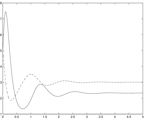
Figure 3.1: Dynamics of $\rho$ (

Remark 3.2

We can rewrite (23) and (21) as

$$\dot{v}=Av+b$$ (30)

where

$$v=\left(\begin{array}[]{c}Q\\ J\end{array}\right),\qquad A=\left(\begin{array}[]{cc}0&-\alpha\\ 1&-1\end{array}\right),\qquad b=\left(\begin{array}[]{c}\int nR^{2}\,dx\\ 0\end{array}\right).$$ (31)

For $\beta$ small $A$ has real eigenvalues whereas for $\beta$ large, it has complex eigenvalues. Therefore our method cannot work for $\beta$ large. One direction to extend the result would be to work directly on the system (23)–(21).

4 Perspectives and open questions

We have proved long term convergence to an ESD for a general model of a chemostat where the nurient delivery does not react immediately to the population dynamics. Our proof extends the proof based on Total Variation bounds developed in [13, 2, 14] and uses a fast (but not infinite) nutrient production measured by the small parameter $\beta$.

Surprisingly, the proof does not seem to give directly uniform TV bounds for $\beta\approx 0$. It does not seem to be possible with this approach to prove uniform bounds for the full range $\beta\in[0,\beta_{0}]$ for some small $\beta_{0}$, which could be a first step to prove uniform convergence of $S(t)$ for $t\in[0,\infty]$ as $\beta\to 0$.

There are several related problems which, usually, can be approached with the same method. One of them is the rare mutations/long term behaviour described by the following extension of (5)–(7)

$$\left\{\begin{array}[]{l}\varepsilon\partial_{t}n_{\varepsilon}(t,x)-\varepsilon^{2}\Delta n_{\varepsilon}=n_{\varepsilon}\,R(x,S_{\varepsilon}(t)),\qquad x\in\mathbb{R}^{d},\;t\geq 0,\\[5.0pt] \varepsilon\beta\frac{d}{dt}S_{\varepsilon}(t)=Q\big{(}S_{\varepsilon}(t),\rho_{\varepsilon}(t)\big{)},\\[5.0pt] \rho_{\varepsilon}(t):=\int n_{\varepsilon}(t,x)\,dx,\end{array}\right.$$

which can be treated using the constrained Hamilton-Jacobi approach [8, 13, 2, 14, 11], provided some strong compactness is proved as e.g. TV bounds which are uniform in $\varepsilon$.

From the modelling side, the TV bounds giving long term behaviour is not known in several examples of chemostat systems. An example is the quasi-stationary case with general uptake rate and rendering factor,

$$\left\{\begin{array}[]{l}\partial_{t}n=nR(x,S),\\[5.0pt] S+\int\eta(x,S)n(x)\,dx=S_{0}.\end{array}\right.$$

Acknowledgment. This research was supported by the french ”ANR blanche” project Kibord: ANR-13-BS01-0004.

References

• [1] Azmy S. Ackleh, Ben G. Fitzpatrick, and Horst R. Thieme. Rate distributions and survival of the fittest: a formulation on the space of measures. Discrete Contin. Dyn. Syst. Ser. B, 5(4):917–928 (electronic), 2005.
• [2] G. Barles and B. Perthame. Concentrations and constrained Hamilton-Jacobi equations arising in adaptive dynamics. Contemp. Math., 439:57–68, 2007.
• [3] N. Brunel and V. Hakim. Fast global oscillations in networks of integrate-and-fire neurons with low firing rates. Neural Comput., 11(7):1621–1671, October 1999.
• [4] N. Champagnat, P.-E. Jabin, and G. Raoul. Convergence to equilibrium in competitive lotka-volterra equations and chemostat systems. C. R. Acad. Sci. Paris Sér. I Math., 348(23-24):1267–1272, 2010.
• [5] R. Cressman and J. Hofbauer. Measure dynamics on a one-dimensional continuous trait space: theoretical foundations for adaptive dynamics. Th. Pop. Biol., 67(1):47–59, 2005.
• [6] L. Desvillettes, P.-E. Jabin, S. Mischler, and G. Raoul. On mutation-selection dynamics for continuous structured populations. Commun. Math. Sci., 6(3):729–747, 2008.
• [7] O. Diekmann. A beginner’s guide to adaptive dynamics. In Mathematical modelling of population dynamics, volume 63 of Banach Center Publ., pages 47–86. Polish Acad. Sci., Warsaw, 2004.
• [8] O. Diekmann, P.-E. Jabin, S. Mischler, and B. Perthame. The dynamics of adaptation: an illuminating example and a Hamilton-Jacobi approach. Th. Pop. Biol., 67(4):257–271, 2005.
• [9] S. A. H. Geritz, E. Kisdi, G. Mészena, and J. A. J. Metz. Evolutionarily singular strategies and the adaptive growth and branching of the evolutionary tree. Evol. Ecol, 12:35–57, 1998.
• [10] P.-E. Jabin and G. Raoul. On selection dynamics for competitive interactions. J. Math. Biol., 63(3):493–517, 2011.
• [11] A. Lorz, S. Mirrahimi, and B. Perthame. Dirac mass dynamics in multidimensional nonlocal parabolic equations. Comm. Partial Differential Equations, 36(6):1071–1098, 2011.
• [12] S. Mirrahimi, B. Perthame, and J. Y. Wakano. Direct competition results from strong competition for limited resource. Preprint.
• [13] B. Perthame. Transport equations in biology. Frontiers in Mathematics. Birkhäuser Verlag, Basel, 2007.
• [14] B. Perthame and G. Barles. Dirac concentrations in Lotka-Volterra parabolic PDEs. Indiana Univ. Math. J., 57(7):3275–3301, 2008.
• [15] H. L. Smith and P. Waltman. The theory of the chemostat: dynamics of microbial competition. Cambridge Univ. Press, 1994.
• [16] R. W. Sterner and J. J. Elser. Ecological Stoichiometry: The Biology of Elements from Molecules to the Biosphere. Princeton University Press, 2002.