Analytic Evolution of Singular Distribution Amplitudes in QCD

Abstract

We describe a method of analytic evolution of distribution amplitudes (DA) that have singularities, such as non-zero values at the end-points of the support region, jumps at some points inside the support region and cusps. We illustrate the method by applying it to the evolution of a flat (constant) DA, antisymmetric flat DA and then use it for evolution of the two-photon generalized distribution amplitude. Our approach has advantages over the standard method of expansion in Gegenbauer polynomials, which requires infinite number of terms in order to accurately reproduce functions in the vicinity of singular points, and over a straightforward iteration of an initial distribution with evolution kernel. The latter produces logarithmically divergent terms at each iteration, while in our method the logarithmic singularities are summed from the start, which immediately produces a continuous curve, with only one or two iterations needed afterwards in order to get rather precise results.

I Introduction

Construction of theoretical models for Generalized Parton Distributions (GPDs) Mueller et al. (1994); Ji (1997); Radyushkin (1996); Collins et al. (1997) is an inherent part of their studies. These models should satisfy several nontrivial requirements that follow from most general principles of quantum field theory. In this context, one could mention polynomiality Ji (1998), positivity Martin and Ryskin (1998); Pire et al. (1999); Radyushkin (1999), hermiticity Mueller et al. (1994), time reversal invariance Ji (1998), etc. These complicated conditions, however, are automatically satisfied by relevant Feynman diagrams of perturbation theory. In particular, analysis of simple one-loop diagrams is the basis of the factorized DD Ansatz Radyushkin (1999) that is a standard element of codes generating models for GPDs.

In fact, the commonly used version of the factorized DD Ansatz involves the assumption about universality of the DD profile function, which, though supported by one-loop examples, was not shown to be a mandatory property of double distributions. A possible way to go beyond the one-loop analysis, but still remain within the perturbation theory framework, is to incorporate pQCD evolution equations. Namely, the strategy is to take the expression for some one-loop diagram as the starting function for evolution, and use evolved patterns for modeling GPDs.

Implementation of such a program faces some technical difficulties. In particular, a well known property of GPDs $H(x,\xi)$ is that they are non-analytic at border points $x=\pm\xi$. For one-loop diagrams, this non-analyticity may take the form of cusps, jumps, and even delta-functions. Thus, one needs to develop methods of evolution for singular initial distributions. A simple example of a singular distribution is given by flat distribution amplitudes $\varphi(x)=$ const which do not vanish at the $x=0,x=1$ boundaries of the DA support region. In our work Tandogan and Radyushkin (2011), we proposed a method that allows to easily establish the major evolution pattern $(x\bar{x})^{t}$ for a flat DA, and provides an algorithm for an analytic calculation of corrections to it. The method was also applied to a DA $\varphi(x)={\rm sgn}(x-1/2)$ that has a jump at $x=1/2$, in the middle of the support interval, with DA being antisymmetric with respect to that point.

In the present paper, we describe the method of analytic evolution of singular distribution amplitudes outlined in Ref. Tandogan and Radyushkin (2011), and extend it for studying evolution of generalized distribution amplitudes (GDAs) Diehl et al. (1998) (our preliminary results on this application have been reported in Ref. Tandogan and Radyushkin (2014)). Similarly to GPDs, these functions are non-analytic at kinematics-dependent points $x=\zeta,1-\zeta$ inside the support interval. The evolution of GPDs is further complicated by the fact that GPD evolution kernels also depend on skewness $\zeta$ (or $\xi$). Unlike GPDs, GDAs evolve according to the same $\zeta$-independent Efremov-Radyushkin-Brodsky-Lepage (ERBL) evolution equation Efremov and Radyushkin (1980); Lepage and Brodsky (1980) as usual DAs, which allows us to concentrate on studying implications due to the non-analytic structure of the initial distribution. A particular object that we consider is the two-photon GDA Pire and Szymanowski (2003) related to the reaction $\gamma^{\ast}(q)\gamma(q^{\prime})\rightarrow\gamma(p_{1})\gamma(p_{2})$. In the QCD lowest order, it is proportional to the $VV\to VV$ ERBL evolution kernel, but the evolution of its $\ln Q^{2}$ derivative, in the leading logarithm approximation, is governed by the $qq\to qq$ ERBL kernel, just as in examples considered in Ref. Tandogan and Radyushkin (2011).

The paper is organized as follows. In Sec. II, we discuss the basic ideas of our method. In particular, we convert the evolution equation to the form in which the convolution integral has the structure of the “plus prescription” with respect to the integration variable $y$. The equation is further simplified by choosing the Ansatz that absorbs the extra term that generates terms logarithmically singular at the end-points of the support region. Applying this method for initially flat DA, we find that, for whatever small positive value of the evolution parameter $t$, the flat DA evolves into a function vanishing at the end points with its shape dominated by the $(x\bar{x})^{t}$ factor. Then we analytically calculate the lowest corrections to this approximation. We also apply this method to the antisymmetric flat DA that initially takes opposite values for $x<1/2$ and $x>1/2$. Such a DA is the simplest example of initial distribution with a jump inside the support region, in this case in the middle of the region. For further applications, we consider the case of an antisymmetric jump ($\phi(x=\zeta_{-})=-\phi(x=\zeta_{+})$ at an arbitrary position $x=\zeta$ inside the support region, and derive the formulas that are used in Secs. III-V, where we apply the approach to the evolution of the two-photon generalized distribution amplitude $\psi^{q}(x,\zeta,Q^{2})$. Its logarithmic derivative with respect to $Q^{2}$ satisfies the ERBL evolution equation, with initial conditions given by a function $\varphi(x,\zeta)$ that has both jumps (discontinuities in the value of the function $\varphi(x,\zeta)$) and cusps (discontinuities in the value of the derivative $\partial\varphi(x,\zeta)/\partial x$)) at the “border” points $x=\zeta,x=1-\zeta$. The structure of $\varphi(x,\zeta)$ is discussed in Sec. III, where it is proposed to split it into a part that has antisymmetric jumps at the border points, and a continuous remainder that has cusps there. Evolution of the “jump” part of two-photon GDA is considered in Sec. IV, while evolution of the “cusp” part is considered in Sec. V. Finally, we summarize the paper.

II Evolution of Singular Distribution Amplitudes

II.1 Evolution equation: basics

Our goal is to study ERBL evolution of distribution amplitudes (DAs) having singularities, with particular emphasis on the analytical investigation of the behavior of evolved amplitudes in the vicinity of singular points. Specifically, we will analyze the evolution governed by the nonsinglet quark-quark ERBL kernel. Particular examples of DAs whose evolution is described by this kernel include pion DA, $\rho$-meson DA and (logarithmic derivative of) nonsinglet two-photon GDAs. In the leading logarithm approximation, the relevant ERBL evolution equation Efremov and Radyushkin (1980); Lepage and Brodsky (1980) reads

$$\frac{\partial\varphi(x,t)}{\partial t}=\int_{0}^{1}[V(x,y)]_{+}\,\varphi(y,t)dy,$$ (1)

where $t=2C_{F}\ln\ln(\mu/\Lambda)/b_{0}$ is the leading logarithm QCD evolution parameter,

$$V(x,y)= \left[\frac{x}{y}\left(1+\frac{1}{y-x}\right)\right]\theta(x<y)$$

$$+\left[\frac{\bar{x}}{\bar{y}}\left(1+\frac{1}{x-y}\right)\right]\theta(y<x)$$ (2)

is the evolution kernel (we use $\bar{x}=1-x$ and $\bar{y}=1-y$), which has singularity for $x=y$ regulated by the plus prescription

$$[V(x,y)]_{+}=V(x,y)-\delta(y-x)\int_{0}^{1}V(z,y)dz$$ (3)

with respect to the first argument $x$. In explicit form the evolution equation is

$$\frac{\partial\varphi(x,t)}{\partial t}=\int_{0}^{1}\left[V(x,y)\varphi(y,t)-V(y,x)\,\varphi(x,t)\right]\,dy\ .$$ (4)

The usual approach Efremov and Radyushkin (1980); Lepage and Brodsky (1980) to solve ERBL equation is to expand initial DA over the eigenfunctions $x(1-x)C_{n}^{3/2}(2x-1)$ of the evolution kernel. Each Gegenbauer projection then changes as a power $t^{-\lambda_{n}}$ of the evolution parameter. All anomalous dimensions $\lambda_{n}$ are positive, except for $\lambda_{0}$ which is zero, hence only the $\sim x(1-x)$ part survives for $t\to\infty$. For a pion DA given by a sum of a few Gegenbauer polynomials, this method gives a convenient analytic expression for the DA evolution. However, if the initial DA does not vanish at the end points, or has jumps inside the support region, one should formally take an infinite number of Gegenbauer polynomials. In practice, this means that one should sum over a large number of terms to get a reasonably precise (point by point) result for the evolved DA.

Another way is to solve the evolution equation by iterations, i.e. write the solution as a series expansion

$$\varphi(x,t)=\sum_{n=0}^{\infty}\frac{t^{n}}{n!}\,\varphi_{n}(x)\ ,$$ (5)

with the functions $\varphi_{n}(x)$ satisfying the recurrence relation

$$\varphi_{n+1}(x)=\int_{0}^{1}\left[V(x,y)\varphi_{n}(y)-V(y,x)\,\varphi_{n}(x)\right]\,dy\ .$$ (6)

II.2 Evolution of flat DA

Taking flat DA $\varphi^{F}_{0}(x)=1$ as the simplest example of the function that does not vanish at the end points, one finds that the first iteration

$$\varphi^{F}_{1}(x)= \int_{0}^{1}[V(x,y)-V(y,x)]dy$$

$$=3/2+x\ln\bar{x}+\bar{x}\ln x\equiv v(x)$$ (7)

has logarithmic singularities $\ln x$ and $\ln\bar{x}$ at the end points. In fact, they just reflect the $t$-expansion of a regular function $(x\bar{x})^{t}$ that appears as the all-order summation result, and has a power behavior at the end points. It is easy to obtain that the singular, logarithmic part of $\varphi_{1}^{F}(x)$ comes from the singular $1/(x-y)$ part of the QCD evolution kernel, which contributes $2+\ln(x\bar{x})$ into the iteration result.

The singularities of $V(x,y)$ and $V(y,x)$ at $x=y$ cancel each other in the integrand of the evolution equation (4), even though the subtraction procedure in this integral does not look like a “+”-prescription with respect to the integration variable “$y$”. But one can rewrite (4) as

$$\frac{\partial\varphi(x,t)}{\partial t}= \int_{0}^{1}V(x,y)[\varphi(y,t)-\varphi(x,t)]dy$$

$$+\varphi(x,t)\int_{0}^{1}[V(x,y)-V(y,x)]dy\ ,$$ (8)

where the first term has the desired structure of the “+”-prescription with respect to $y$. The integral in the second term coincides with the first iteration of the evolution kernel with the flat DA denoted in (7) by $v(x)$, i.e., we can write

$$\frac{\partial\varphi(x,t)}{\partial t}= \int_{0}^{1}V(x,y)[\varphi(y,t)-\varphi(x,t)]dy$$

$$+v(x)\,\varphi(x,t)\ .$$ (9)

The evolution equation (9) can be simplified through taking the Ansatz

$$\varphi(x,t)=e^{tv(x)}\Phi(x,t)\ ,$$ (10)

resulting in

$$\frac{\partial{\Phi(x,t)}}{\partial t}=\int_{0}^{1}V(x,y)\,\left[e^{t[v(y)-v(x)]}\Phi(y,t)-\Phi(x,t)\right]\,dy\,.$$ (11)

Expanding

$$\Phi(x,t)=\sum_{n=0}^{\infty}\frac{t^{n}}{n!}\Phi_{n}(x)$$ (12)

gives the recurrence relations

$$\Phi_{n+1}(x)=\int_{0}^{1}V(x,y) \Biggl{\{}\sum_{l=0}^{n}\frac{n!\,\Phi_{l}(y)}{(n-l)!\,l!}\left[v(y)-v(x)\right]^{n-l}-\Phi_{n}(x)\Biggr{\}}dy\ .$$ (13)

Keeping only the singular part of the evolution kernel, i.e., using $v^{\rm sing}(x)=2+\ln(x\bar{x})$, we obtain for the first terms,

$$\Phi_{1}^{\rm sing} (x)=\int_{0}^{1}V(x,y)[\Phi_{0}(y)-\Phi_{0}(x)]dy\,,$$

$$\Phi_{2}^{\rm sing} (x)=\int_{0}^{1}V(x,y)\bigl{[}\Phi_{0}(y)\ln\left(\frac{y\bar{y}}{x\bar{x}}\right)+\Phi_{1}(y)-\Phi_{1}(x)\bigr{]}dy\,,$$

$$\Phi_{3}^{\rm sing} (x)=\int_{0}^{1}V(x,y)\left[\Phi_{0}(y)\ln^{2}\left(\frac{y\bar{y}}{x\bar{x}}\right)+2\Phi_{1}(y)\ln\left(\frac{y\bar{y}}{x\bar{x}}\right)+\Phi_{2}(y)-\Phi_{2}(x)\right]dy\,.\ \ \$$ (14)

For the flat initial DA, i.e., $\Phi(x,0)=1$, the first correction $\Phi_{1}(x)$ vanishes, $\Phi_{1}(x,0)=0$, and then

$$\Phi_{2}^{\rm sing}(x) =-2\ln x\ln\bar{x}\ ,$$ (15)

$$\Phi_{3}^{\rm sing}(x) =3\ln(x\bar{x})\ln x\ln\bar{x}+2\left[\ln x\,\text{Li}_{2}(x)+\ln\bar{x}\,\text{Li}_{2}(\bar{x})\right]-4\,\left[\text{Li}_{3}(x)+\,\text{Li}_{3}(\bar{x})\right]+8\zeta(3)\ .$$ (16)

For the total kernel, when $v(x)=3/2+x\ln\bar{x}+\bar{x}\ln x$, we have

$$\Phi_{2}(x)= x\ln x[1+(x-1/2)\ln x]+\bar{x}\ln\bar{x}[1+(x+1/2)\ln\bar{x}]-\ln x\ln\bar{x}+x\text{Li}_{2}\left(-\frac{\bar{x}}{x}\right)+\bar{x}\text{Li}_{2}\left(-\frac{x}{\bar{x}}\right)$$ (17)

for the second iteration. The third iteration in this case is given by a rather long expression.

II.3 Normalization

As far as

$$\int_{0}^{1}[V(x,y)]_{+}dx=0\ ,$$

evolution does not change the normalization integral for $\varphi(x,t)$. In particular, if we expand $\varphi(x,t)$ in $t$

$$\varphi(x,t)=\sum_{n=0}^{\infty}\varphi_{n}(x)\,\frac{t^{n}}{n!}\ ,$$ (18)

we should have

$$\int_{0}^{1}\varphi_{n}(x)\,dx=\delta_{n0}\ .$$ (19)

However, when we take the singular kernel case Ansatz

$$\varphi^{\rm sing}(x,t)=e^{t(2+\ln(x\bar{x}))}\Phi(x,t)\ ,$$

the $(t\ln x\bar{x})^{N}$ terms are summed to all orders, while the series over $\varphi_{n}(x)$ is restricted to some finite order $N$. As a result, the approximants $\varphi_{(N)}(x,t)$ are not normalized to 1. In particular, if we keep the terms up to $\Phi_{2}(x)$, the normalization integral is given by

$$I_{2}(t) \equiv\int_{0}^{1}\varphi_{(2)}^{\text{sing}}(x,t)\,dx=e^{2t}\frac{\Gamma^{2}(1+t))}{\Gamma(2+2t)}\left\{1-t^{2}\left[(H_{t}-H_{1+2t})^{2}-\psi_{1}(2+2t)\right]\right\}\ \ \$$ (20)

with $H_{n}$ being harmonic numbers and $\psi_{k}$ the polygamma function. One can check that $I_{2}(t)=1+{\cal O}(t^{3})$. For the next approximation, i.e., for $\varphi_{(3)}^{\text{sing}}(x,t)$, the normalization integral is $I_{3}(t)=1+{\cal O}(t^{4})$, etc. For $\varphi_{(N\rightarrow\infty)}(x,t)$, the normalization integral $I_{N}(t)$ will tend to 1 for all $t$.

The normalization integrals versus $t$ are shown in Fig.1a. For approximations involving $\Phi_{0}(x)$ and $\Phi_{2}(x)$, the calculations were done analytically, while the curve corresponding to inclusion of $\Phi_{3}^{\text{sing}}(x,t)$ was calculated numerically. As seen from Fig.1a, adding more terms brings normalization closer to $1$.

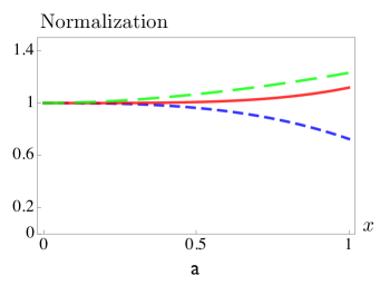
Figure 1: a) Normalization factor calculated for terms including only $\Phi_{0}(x)$ (short-dashed line), $\Phi_{0}(x)$ and $\Phi_{2}(x)$ (long-dashed line) and $\Phi_{0}(x)$, $\Phi_{2}(x)$ and $\Phi_{3}(x)$ (solid line). b) Evolution of the flat DA under the singular part of the evolution kernel: the curves shown correspond to $t=0,t=0.3,t=0.6,t=1.0$.

In this situation, it makes sense to introduce the “normalized Ansatz”, in which $\varphi(x,t)$ is approximated by the ratio

$$\nu_{N}(x,t)\equiv\varphi_{(N)}(x,t)/I_{N}(t)\ ,$$

so that the correct normalization of the $N$th approximant is guaranteed for all $t$. In particular, this gives

$$\nu_{2}(x,t)= (x\bar{x})^{t}\,\frac{\Gamma(2+2t)}{\Gamma^{2}(1+t)}\frac{1-t^{2}\ln x\,\ln\bar{x}}{1-t^{2}\left[(H_{t}-H_{1+2t})^{2}-\psi_{1}(2+2t)\right]}\ .$$ (21)

As seen from this formula (and also from Fig.1b), the initial flat function immediately (for whatever small positive $t$) evolves into a function vanishing at the end points with its shape dominated by the $(x\bar{x})^{t}$ factor.

In case of the total kernel, we have

$$\varphi_{(2)}(x,t)= e^{3t/2}\,(x^{\bar{x}}\bar{x}^{x})^{t}\left(1+\frac{t^{2}}{2!}\Phi_{2}(x)\right)\ .$$ (22)

Unfortunately, for this form it is impossible to analytically calculate the normalization integral even for the lowest term. Compared to the Ansatz used for the singular part of the evolution kernel, the Ansatz

$$\varphi(x,t)=e^{tv(x)}\Phi(x,t)=e^{3t/2}(x^{\bar{x}}\bar{x}^{x})^{t}\Phi(x,t)$$ (23)

has an extra overall factor $[e^{-1/2}x^{-x}\bar{x}^{-\bar{x}}]^{t}\ .$ Note that the function $x^{-x}\bar{x}^{-\bar{x}}$ is finite at the end points $x=0,\,1$, where it takes its minimal value for the interval $[0,1]$ (equal to 1), and has a maximum for $x=1/2$, where it equals 2. Thus, the factor $e^{-1/2}x^{-x}\bar{x}^{-\bar{x}}$ enhances the $x\bar{x}$ profile in the middle (by $2/\sqrt{e}\approx 1.2$ factor) and suppresses it at the end points (by $1/\sqrt{e}\approx 0.6$). This is a rather mild modification, and what is most important, it does not change the $\sim x^{t}$ (or $\sim\bar{x}^{t}$) behavior at the end points. So, it makes sense to use the expansion

$$[x^{-x}\bar{x}^{-\bar{x}}]^{t}=\sum_{n=0}^{\infty}(-1)^{n}(x\ln x+\bar{x}\ln\bar{x})^{n}\,\frac{t^{n}}{n!}\ ,$$ (24)

in powers of $t$ and combine it with the expansion for $\Phi(x,t)$.

This corresponds to Ansatz

$$\varphi(x,t)= (x\bar{x})^{t}\,e^{3t/2}\,\left[\tilde{\Phi}_{0}(x)+t\,\tilde{\Phi}_{1}(x)+\frac{t^{2}}{2!}\tilde{\Phi}_{2}(x)+\ldots\right]\ ,$$ (25)

whose expansion coefficients $\tilde{\Phi}_{n}(x)$ can be straightforwardly obtained from $\Phi_{n}(x)$’s calculated using $v^{\rm sing}(x)$. In particular,

$$\tilde{\Phi}_{1}(x)= -(x\ln x+\bar{x}\ln\bar{x})\ ,$$ (26)

$$\tilde{\Phi}_{2}(x)= \Phi_{2}(x)+(x\ln x+\bar{x}\ln\bar{x})^{2}\ .$$ (27)

For the lowest terms, we can analytically calculate the normalization integral:

$$I_{1}(t)\equiv \int_{0}^{1}\varphi_{(1)}(x,t)dx=e^{3t/2}\frac{\Gamma^{2}(1+t)}{\Gamma(2+2t)}\left(1-\frac{t}{2(t+1)}+\frac{t}{2}(-H_{t}+H_{1+2t})\right)\!,$$ (28)

where $H_{n}$ are harmonic numbers. Fig.2a shows the normalization versus $t$.

Again, we may switch to the normalized Ansatz formed by the ratio $\varphi_{(N)}(x,t)/I_{N}(t)$. For a flat initial distribution, this gives

$$\nu_{1}(x,t) =(x\bar{x})^{t}\,\frac{\Gamma(2+2t)}{\Gamma^{2}(1+t)}\frac{1-t\,(x\ln x+\bar{x}\ln\bar{x})}{1-{t}/{2(t+1)}+{t}(-H_{t}+H_{1+2t})/2}\ .$$ (29)

The results are illustrated by Fig.2b.

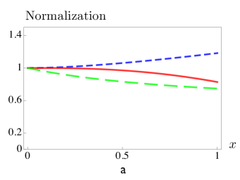
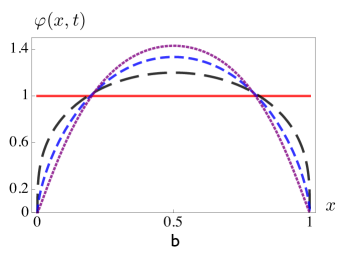
Figure 2: Same as Fig. 1 for the case of full kernel.

II.4 Evolution of Anti-Symmetric Flat DA

II.4.1 Singular Part

Evolution equations may be applied also in situations when the distribution amplitude is antisymmetric with respect to the change $x\to 1-x$. An interesting example is the $D$-term function $d(x)$ that appears in generalized parton distributions. Thus, let us consider evolution of the DA that initially has the form

$$\varphi_{0}(x)=\begin{cases}\,\,\,\,1&0<x\leqslant 1/2\ ,\\ -1&1/2<x<1\ .\end{cases}$$

The $v(x)$ function is the same, since it depends on the kernel $V(x,y)$ only. Thus we can use the Ansatz (10) and expansion (5). Since $\varphi_{0}(x)$ is not just a constant, the first expansion coefficient $\Phi_{1}(x)$ is nonzero. Let us start with the singular part of the kernel. Then we get

$$\Phi_{1}(x)=\begin{cases}-2\ln\left[\frac{\bar{x}}{1-2x}\right]&0<x\leqslant 1/2\ ,\\ \,\,\,\,\,2\ln\left[\frac{x}{-1+2x}\right]&1/2<x\leqslant 1\ .\end{cases}$$

We see that there are logarithmic terms $\ln|1-2x|$ singular for $x=1/2$. These terms are natural, since each half of the antisymmetric DA on its interval is expected to evolve similarly to a flat DA on the $0\leq x\leq 1$ interval. This observation suggests the Ansatz

$$\varphi(x,t)=e^{2t}(x\bar{x})^{t}|1-2x|^{2t}\Phi(x,t)\ .$$ (30)

With this definition of $\Phi(x,t)$, the $\ln|1-2x|$ terms are eliminated from $\Phi_{1}(x)$:

$$\Phi_{1}(x)=-2\ln\bar{x}\ \theta(0<x\leqslant 1/2)-\{x\to\bar{x}\}\ .$$ (31)

For the expansion component $\Phi_{2}(x)$, we have

$$\Phi_{2}(x)= \theta(0<x\leqslant 1/2)\Biggl{\{}-\frac{2\pi^{2}}{3}+5\ln^{2}\bar{x}+\ln(1-2x)[4\ln 2+4\ln x-2\ln\bar{x}+\ln(1-2x)]-2\ln\bar{x}\ln x$$

$$-4\text{Li}_{2}(x)+4\text{Li}_{2}(2x)+2\text{Li}_{2}\left[\frac{x}{\bar{x}}\right]+2\text{Li}_{2}\left[\frac{x}{2x-1}\right]+4\text{Li}_{2}\left[\frac{1-2x}{\bar{x}}\right]\Biggr{\}}-\{x\to\bar{x}\}\ .$$ (32)

The graphical results for the expansion components are shown in Fig.3a,b).

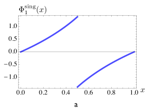
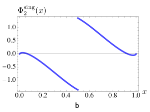
Figure 3: Expansion components $\Phi^{\text{sing}}_{1}(x)$ (a) and $\Phi^{\text{sing}}_{2}(x)$ (b) for the antisymmetric DA in case of singular part of the kernel; c) evolution of antisymmetric DA under the singular part of the kernel for $t=0,t=0.3,$ $t=0.6,t=1$.

The evolution of $\varphi_{\text{sing}}(x,t)$ to this accuracy can be obtained from

$$\varphi(x,t)= e^{2t}(x\bar{x})^{t}|1-2x|^{2t}\left(\varphi_{0}(x)+t\Phi_{1}(x)+\frac{t^{2}}{2!}\Phi_{2}(x)\right)\ .$$ (33)

As shown in Fig.3c, the initial step function evolves into a function which is zero at the end points and in the middle point.

II.5 Adding Non-Singular Part of the Kernel

Since the nonsingular part does not add $\ln x$ and $\ln\bar{x}$ terms to $v(x)$, we may proceed with the same Ansatz

$$\varphi(x,t)= e^{3t/2}(x\bar{x})^{t}|1-2x|^{2t}\Phi(x,t)\,,$$ (34)

but the expansion components change (see Fig.4a,b).

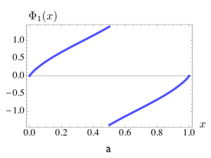
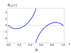
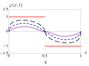
Figure 4: Expansion components $\Phi_{1}(x)$ (a) and $\Phi_{2}(x)$ (b) in the case of the full kernel; c) evolution of the antisymmetric DA in the full kernel case for $t=0,$ $t=0.3,t=0.6,t=1$.

The distribution amplitude is now built using

$$\varphi(x,t)= e^{3/2t}(x\bar{x})^{t}|1-2x|^{2t}\left(\varphi_{0}(x)+t\Phi_{1}(x)+\frac{t^{2}}{2!}\Phi_{2}(x)\right),$$ (35)

For the first coefficient we have

$$\Phi_{1}(x)=\theta(0<x\leqslant 1/2)\bigl{\{}-2x\ln 2-2\ln\bar{x}-(\bar{x}\ln\bar{x}+x\ln x)\bigl{\}}-\{x\to\bar{x}\}\ ,$$ (36)

and for the second,

$$\Phi_{2}(x)= \theta(0<x\leqslant 1/2)\Biggl{\{}-\frac{\pi^{2}}{2}\bar{x}+2\ln^{2}+2x\ln 2+\ln\bar{x}[2+8\ln 2+17\ln\bar{x}]-(x-2\ln(1-2x)[\ln\bar{x}-\ln x]$$

$$+2(5x-3)\ln 2\ln(1-2x)-\ln^{2}(1-2x)-6x\ln^{2}\bar{x}+\ln\bar{x}\ln x+x\ln x(4\ln 2+\ln\bar{x}+\ln x$$

$$+2\ln(1-2x)+2\ln\bar{x})+2\bar{x}\bigg{[}\text{Li}_{2}\left(\frac{1-2x}{2\bar{x}}\right)+\text{Li}_{2}\left(\frac{1-2x}{\bar{x}}\right)+\text{Li}_{2}(x)-\text{Li}_{2}(2x)\bigg{]}$$

$$-(1+2x)\text{Li}_{2}\left(-\frac{x}{\bar{x}}\right)+\text{Li}_{2}\left(\frac{x^{2}}{\bar{x}^{2}}\right)-2\text{Li}_{2}\left(\frac{x}{2x-1}\right)\Biggl{\}}-\{x\to\bar{x}\}\ .$$ (37)

As may be seen from Fig.4c, the resulting curves are rather close to those obtained when only singular part of the kernel was taken into account. Thus, we observe that the $t^{n}$ series converges rather rapidly as far as $t\lesssim 1$. When $t\gtrsim 1$, the DAs is close to the asymptotic form, and one can switch to the solution in the form of Gegenbauer expansion.

II.6 Evolution of jumps

Another example of singularity is given by DAs with a jump, the simplest case being

$$\Phi^{J}_{0}(x,\zeta;a,b)=\begin{cases}\,\,\,\,a&0<x\leqslant\zeta\ ,\\ \,\,\,\,b&\zeta<x<1\ .\end{cases}$$

The part of the first iteration $\Phi_{1}(x)$ generated by the singular part of the kernel

$$\Phi^{J\,{\rm sing}}_{1}(x,\zeta;a,b)=\begin{cases}\,\,\,\,\,(a-b)\ln\left[\frac{\zeta-x}{(1-x)\zeta}\right]&0<x\leqslant\zeta\ ,\\ \,-(a-b)\ln\left[\frac{x-\zeta}{(1-\zeta)x}\right]&\zeta<x\leqslant 1\end{cases}$$

contains logarithmic terms $\ln|\zeta-x|$ singular for $x=\zeta$. Their structure may be understood in the following way. The original function $\varphi^{J}_{0}(x,\zeta;a,b)$ may be represented as a sum of a constant $\frac{1}{2}(a+b)$ and a function $\frac{1}{2}(a-b){\rm sgn}(\zeta-x)$ that jumps by $b-a$ at the point $x=\zeta$. The constant part has no singularities at $x=\zeta$, so one can apply the original $\frac{1}{2}(a+b)(x\bar{x})^{t}\Phi$ Ansatz to it, while for the jumping part one may use the Ansatz

$$\Phi^{J} (x,\zeta;a,b;t)=\frac{a-b}{2}e^{2t}(x\bar{x})^{t}\left[\left(\frac{1-x/\zeta}{1-x}\right)^{2t}\theta(x<\zeta)\right.$$

$$\left.+\left(\frac{1-\bar{x}/\bar{\zeta}}{1-\bar{x}}\right)^{2t}\theta(x>\zeta)\right]\Phi(x,\zeta)+\Psi(x,\zeta,t)\ .$$ (38)

The part containing square brackets is intended to take care of the evolution of the jump at $x=\zeta$. However, this part by construction vanishes at $x=\zeta$, while one would expect that evolution tends to convert $\varphi^{J}(x,\zeta;a,b)$ into a universal $\zeta$-independent function proportional to $x\bar{x}$ or $x\bar{x}(1-2x)$ (depending on the symmetry of the function). Thus, there should be also a part regular at the jump point. The function $\Psi(x,\zeta,t)$ is introduced to satisfy this requirement. It vanishes for $t=0$, but eventually becomes the dominant part.

Let us discuss a more general case, when a function has antisymmetric jumps at some locations $x=\zeta_{i}$. “Antisymmetric” means that the function approaches opposite values on the sides of a jump, so that “on average” it is zero at the jump points. Then one can try the Ansatz

$$\varphi(x,t)=\Phi(x,t)+\Psi(x,t)\ ,$$ (39)

where

$$\Phi(x,t)=e^{t[v(x)+w(x)]}\Phi_{0}(x)\ ,$$ (40)

with the function $w(x)\sim\sum_{i}\ln|x-\zeta_{i}|$ intended to absorb major features of the evolution of the starting distribution $\varphi(x,t=0)\equiv\Phi_{0}(x)$ in the vicinity of the jump points, while the remainder $\Psi(x,t)$ is expected to be a regular function vanishing for $t=0$. As a result, we get the following equation:

$$\!\!\!\frac{\partial{\Psi(x,t)}}{\partial t}=\int_{0}^{1}\!\!V(x,y)\left[\Psi(y,t)-\Psi(x,t)\right]dy+v(x)\Psi(x,t)$$

$$+\int_{0}^{1}V(x,y)\,\left[\Phi(y,t)-\Phi(x,t)\right]\,dy-w(x)\Phi(x,t)\,.$$ (41)

This is an inhomogeneous evolution equation for $\Psi(x,t)$, with starting condition $\Psi(x,t=0)=0$. For its derivative at $t=0$ we have

$$\left.\frac{\partial{\Psi(x,t)}}{\partial t}\right|_{t=0}= \int_{0}^{1}V(x,y)\,\left[\Phi_{0}(y)-\Phi_{0}(x)\right]\,dy-w(x)\Phi_{0}(x)\equiv\chi(x)\,.$$ (42)

To avoid singularities at the jump points, we should adjust $w(x)$ in such a way as to make $\chi(x)$ a continuous function of $x$. Then $\Psi(x,t)\approx t\chi(x)$ for small $t$. The corrections to this approximation can be found by iterations. Namely, we represent $\Psi(x,t)=\sum_{n=1}\Psi_{n}(x,t)$ and start with

$$\Psi_{1}(x,t)\equiv\int_{0}^{t}d\tau\left\{\int_{0}^{1}V(x,y)\,\left[\Phi(y,\tau)-\Phi(x,\tau)\right]\,dy-w(x)\Phi(x,\tau)\right\}\ ,$$ (43)

generating further terms using

$$\Psi_{n+1}(x,t)\equiv\int_{0}^{t}d\tau\left\{\int_{0}^{1}V(x,y)\,\left[\Psi_{n}(y,\tau)-\Psi_{n}(x,\tau)\right]\,dy+v(x)\Psi_{n}(x,\tau)\right\}\ .$$ (44)

Since the derivative of $\Psi_{1}(x,t)$ for $t=0$ is given by $\chi(x)$, we can write

$$\Psi_{1}(x,t)=t\,\chi(x)+\int_{0}^{t}d\tau\int_{0}^{1}V(x,y)\,\left[\delta\Phi(y,\tau)-\delta\Phi(x,\tau)\right]\,dy-w(x)\delta\Phi(x,\tau)\equiv t\,\chi(x)+\delta\Psi_{1}(x,t)\ .$$ (45)

Here, $\delta\Phi(x,\tau)\equiv\Phi(x,\tau)-\Phi_{0}(x)$ is the deviation of the Ansatz function $\Phi(x,\tau)$ from its $\tau=0$ shape. For small $\tau$, the function $\delta\Phi(x,\tau)$ has a rather sharp behavior at the jump points $x=\zeta_{i}$, and this results in a rather sharp behavior of $\delta\Psi_{1}(x,t)$ at these points. Since each iteration $\Psi_{n+1}(x,t)$ is generated linearly from a previous $\Psi_{n}(x,t)$ one (see Eq. (44) ), it makes sense to split $\Psi(x,t)$ into a “smooth” part $\Psi_{\chi}(x,t)$ generated by iterations of $t\chi(x)$ and the remainder $\delta\Psi(x,t)$ generated by iterations of $\delta\Psi_{1}(x,t)$. Thus, we have

$$\varphi(x,t)=\Phi(x,t)+\delta\Psi(x,t)+\Psi_{\chi}(x,t)\ ,$$ (46)

where the first two terms, $\Phi(x,t)$ and $\delta\Psi(x,t)$ have a rather sharp behavior at the jump points for small $t$, while $\Psi_{\chi}(x,t)$ has a smooth behavior.

III Structure of Two-Photon Generalized Distribution Amplitude

In the lowest QCD order, the non-singlet two-photon GDA is given by El Beiyad et al. (2008)

$$\psi^{q}(x,\zeta,Q^{2}) =\frac{N_{C}\,e_{q}^{2}}{2\pi^{2}}\log{\frac{Q^{2}}{m^{2}}}\,\varphi(x,\zeta)\ ,$$ (47)

where the function $\varphi(x,\zeta)$ is proportional to the $VV\to VV$ component

$$\varphi(x,\zeta) =\frac{\bar{x}(2x-\zeta)}{\bar{\zeta}}\theta(x-\zeta)+\frac{\bar{x}(2x-\bar{\zeta})}{\zeta}\theta(x-\bar{\zeta})-\frac{x(2\bar{x}-\bar{\zeta})}{\zeta}\theta(\zeta-x)-\frac{x(2\bar{x}-{\zeta})}{\bar{\zeta}}\theta(\bar{\zeta}-x)$$ (48)

of the ERBL evolution kernel matrix. QCD corrections induce further evolution of the photon GDA. Namely, its derivative with respect to $\ln Q^{2}$ obeys ERBL evolution equation with the $qq\to qq$ kernel considered above. In what follows, we study ERBL evolution of the function $\varphi(x,\zeta,t)$ which for the starting evolution point $t=0$ coincides with $\varphi(x,\zeta)$.

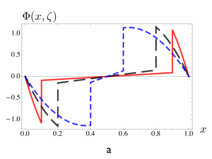
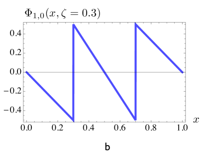
Figure 5: a)Two-photon GDA profile function $\Phi(x,\zeta)$ at values $\zeta=0.1;0.2;0.4$. b) The $x$-profile of the jump part $\Phi_{1,0}(x,\zeta)$ at $\zeta=0.3$.

The function $\varphi(x,\zeta)$ is antisymmetric with respect to $x\leftrightarrow\bar{x}$ interchange and symmetric with respect to $\zeta\leftrightarrow\bar{\zeta}$ interchange. Thus, without loss of generality, we may choose $\zeta\leq 1/2$. Then $0\leq\zeta\leq\bar{\zeta}\leq 1$, and it makes sense to explicitly write the function in each of the three regions:

$$\varphi(x,\zeta)= \left\{\frac{x}{\zeta\bar{\zeta}}\left[\bar{\zeta}^{2}+\zeta^{2}-2\bar{x}\right]\theta(0\leq x\leq\zeta)-\frac{\zeta(1-2x)}{1-\zeta}\theta(\zeta\leq x\leq\bar{\zeta})-\frac{\bar{x}}{\zeta\bar{\zeta}}\left[\bar{\zeta}^{2}+\zeta^{2}-2x\right]\theta(\bar{\zeta}\leq x\leq 1)\right\}\,.$$ (49)

The function is discontinuous at $x=\zeta$ and $x=\bar{\zeta}$. Fig.5a shows the $x$-profile of the two-photon GDA at different $\zeta$ values. As $x$ approaches $\zeta$, the limiting value of the function from the left is $\varphi(\zeta_{-},\zeta)=-1-\zeta\,\frac{1-2\zeta}{1-\zeta}$, while from the right we have $\varphi(\zeta_{+},\zeta)=-\zeta\,\frac{1-2\zeta}{1-\zeta}$, so that the jump $\varphi(\zeta_{+},\zeta)-\varphi(\zeta_{-},\zeta)=1$ is equal to 1. According to our discussion in the preceding section, to treat the evolution of a jump, we should represent the initial function as a sum of a function $\varphi_{2}(x,\zeta)$ continuous in the vicinity of each jump, and a function $\varphi_{1}(x,\zeta)$ that has an antisymmetric jump of necessary size. The function $\varphi_{1}(x,\zeta)$ will also specify the initial form of the $\Phi$-part of the evolution Ansatz (39) for this function, so we will denote it as $\Phi_{1,0}(x,\zeta)$. For simplicity, we will choose it to be given by linear functions of $x$ in each of the three regions. As a result,

$$\Phi_{1,0}(x,\zeta)= -\frac{x}{2\zeta}\theta(0<x<\zeta)+\frac{\bar{x}}{2\zeta}\theta(\bar{\zeta}<x<1)+\frac{1-2x}{2(1-2\zeta)}\theta(\zeta<x<\bar{\zeta})\ .$$ (50)

The function $\Phi_{1,0}(x,\zeta)$ is discontinuous at $x=\zeta$ and $x=\bar{\zeta}$, see Fig.5b, where it is shown for $\zeta=0.3$. The function $\Phi_{2,0}(x,\zeta)$ specifying the initial shape of the continuous part is obtained as the difference between $\varphi(x,\zeta)$ and $\Phi_{1,0}(x,\zeta)$.

IV Evolution of the jump part of two-photon GDA

Iteration of the initial function $\Phi_{1,0}(x,\zeta)$ with evolution kernel gives

$$\Phi_{1,1}(x,\zeta)\equiv \int_{0}^{1}V(x,y)[\Phi_{1,0}(y,\zeta)-\Phi_{1,0}(x,\zeta)]\,dy={\theta(0<x<\zeta<1/2)}\biggl{\{}(1-4\zeta)\,\frac{x}{2\zeta}$$

$$+\frac{1}{2\zeta}\,[x\bar{x}\ln x+(1-x\bar{x})\ln\bar{x}]-\ln(\zeta-x)-\ln(\bar{\zeta}-x)+\frac{\ln\zeta+\ln\bar{\zeta}\,(1-3\zeta)/\zeta}{2(1-2\zeta)}\,\bar{x}$$

$$-\frac{1-4\zeta}{\zeta(1-2\zeta)}\left[(x-\zeta)\ln(\zeta-x)+(\bar{\zeta}-x)\ln(\bar{\zeta}-x)\right]\biggr{\}}-\{x\rightarrow\bar{x}\}$$

$$+{\theta(\zeta<x<\bar{\zeta})}\biggl{\{}\frac{1-2x}{2(1-2\zeta)}\Bigl{[}(1-4\zeta)+\ln\bar{\zeta}\,(1-3\zeta)/\zeta\Bigr{]}+\ln(x-\zeta)-\ln(\bar{\zeta}-x)$$

$$+\frac{1-4\zeta}{2\zeta(1-2\zeta)}\Bigl{[}(x-\zeta)\ln(x-\zeta)-(\bar{\zeta}-x)\ln(\bar{\zeta}-x)+\bar{x}\ln\bar{x}-x\ln x\Bigr{]}+\frac{x^{2}+\bar{x}^{2}}{2(1-2\zeta)}\ln\left(\frac{\bar{x}}{x}\right)\biggr{\}}\ .$$ (51)

As expected, $\Phi_{1,1}(x,\zeta)$ has logarithmic singularities

$$-\ln(\zeta-x)\theta(x<\zeta)+\ln(x-\zeta) \theta\left(\zeta<x<1/2\right)$$

$$-\{x\to\bar{x}\}$$ (52)

for $x=\zeta$ and $x=\bar{\zeta}$ (see Fig.6a). The sum of these terms may be written as $2(\ln|x-\zeta|+\ln|x-\bar{\zeta}|)\Phi_{1}(x,\zeta)$ plus regular terms, which suggests to take the Ansatz (39) with $w(x)$ containing $2(\ln|x-\zeta|+\ln|x-\bar{\zeta}|)$. Namely, let us try the function $w_{0}(x,\zeta)$ given by

$$w_{0}(x,\zeta)=4+2\ln|x-\zeta|+2\ln|x-\bar{\zeta}|\ .$$ (53)

The constant part “4” was chosen to make the integral of $w_{0}(x)$ closer to zero (it vanishes both for $\zeta=0$ and $\zeta=1$), i.e. to keep the overall normalization of the Ansatz factor closer to 1. Resulting function (which gives the first term of the $\Psi$-part of the Ansatz (39)) is given by

$$\Psi_{1,1}^{(0)}(x,\zeta)=\Phi_{1,1}(x,\zeta)-w_{0}(x,\zeta)\Phi_{1}(x,\zeta)$$ (54)

and shown in Fig.6b. One can see that, after the subtraction of singularities, we still have finite jumps for $x=\zeta$ and $x=\bar{\zeta}$. Explicit calculation gives

$$\Psi_{1,1}^{(0)}(\zeta_{+},\zeta) -\Psi^{(0)}_{1,1}(\zeta_{-},\zeta)=4+2\ln(|1-2\zeta|)$$

$$+(2-\zeta)\ln\zeta+(2-\bar{\zeta})\ln\bar{\zeta}\equiv-w_{1}(\zeta)\ .$$ (55)

Adding $w_{1}(\zeta)\Phi_{1,0}(x,\zeta)$ to $\Psi_{1,1}^{(0)}(x,\zeta)$, we obtain the correction function $\Psi_{1,1}(x,\zeta)\equiv\chi(x,\zeta)$ that is continuous at the border points $x=\zeta$ and $x=\bar{\zeta}$ (see Fig.6c).

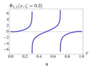
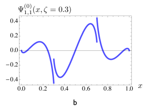
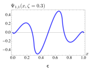
Figure 6: a) First iteration $\Phi_{1,1}(x,\zeta)$ for $\zeta=0.3$. b) Correction functions $\Psi_{1,1}^{(0)}(x,\zeta=0.3)$ with $w_{0}$ Ansatz. c) Correction functions $\Psi_{1,1}^{(0)}(x,\zeta=0.3)$ with modified Ansatz.

This corresponds to the following $\Phi$-part of the Ansatz (39)

$$\Phi_{1}(x,\zeta,t)= e^{tv(x)}\left(\frac{|1-x/\zeta||1-x/\bar{\zeta}|}{|1-2\zeta|}\right)^{2t}\zeta^{t\zeta}\bar{\zeta}^{t\bar{\zeta}}\Phi_{1,0}(x,\zeta)$$ (56)

for the function $\varphi_{1}(x,\zeta,t)$. The function $\Phi_{1}(x,\zeta,t)$ is illustrated in Fig. 7a.

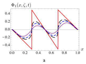
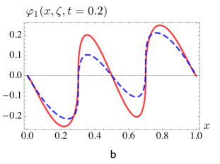
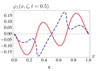
Figure 7: a) Ansatz function $\Phi_{1}(x,\zeta=0.3,t)$ for $t=0,\ 0.2,\ 0.3,\ 0.5$. Effect of inclusion of $\Psi_{1,1}(x,\zeta)$ correction for $t=0.2$ (b) and $t=0.5$ (c); $\zeta=0.3$ in both cases.

According to Ansatz (39), after fixing the function $w(x)$ from the requirement of continuity of $\chi(x,\zeta)$, one should deal with the evolution equation (41) for the $\Psi$-part of the Ansatz. This equation specifies that $\partial\Psi_{1}(x,\zeta,t)/\partial t$ for $t=0$ is given by $\chi(x,\zeta)$. Thus, for small $t$, we can approximate $\Psi_{1}(x,\zeta,t)$ by $t\chi(x,\zeta)$. As one can see from Fig.7b, the correction due to the $\Psi$ term is rather small for $t=0.2$. It just reduces somewhat the amplitude of oscillations.

However, the correction becomes more and more visible with growing $t$, see Fig.7c, where the evolved function is shown for $t=0.4$ with and without the first $\Psi$-type correction term included. The total function is now clearly nonzero at the “border” points $x=\zeta$ and $x=1-\zeta$. This is because $\chi(x,\zeta)$ is nonzero at these points. As we discussed, the $\Psi$-part becomes dominant for large $t$ and brings the shape of $\varphi_{1}(x,\zeta,t)$ to the asymptotic form $x\bar{x}(2x-1)$ of the antisymmetric DAs. We can see that, for $t=0.4$ already, the total function resembles the asymptotic shape $x\bar{x}(2x-1)$. However, for such large $t$ values the simplest linear-$t$ approximation for $\Psi(x,\zeta,t)$ is too crude, and one should go beyond the first iteration.

As argued in the discussion after Eq. (39), it makes sense to split $\Psi(x,,\zeta,t)$ into a part generated by iterations of $t\chi(x,\zeta)$, and the remainder $\delta\Psi(x,,\zeta,t)$ given by iterations of the terms reflecting the deviation $\delta\Phi(x,\zeta;t)\equiv\Phi(x,\zeta;t)-\Phi_{0}(x,\zeta)$ of the Ansatz function $\Phi(x,\zeta;t)$ from its $t=0$ form $\Phi_{0}(x,\zeta)$. The starting term $\delta\Psi_{1}(x,,\zeta,t)$ has a sharp behavior at the jump points of $\Phi_{0}(x,\zeta)$ (see Fig. 8a), acquiring an infinite slope there as $t\to 0$. Up to this point of the calculation, all iterations are calculated analytically, however the next iteration, $\delta\Psi(x\zeta,t)$ (see Fig. 8b) was calculated numerically.

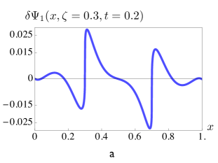
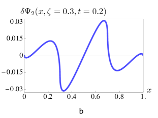
Figure 8: a) $\delta\Psi_{1}(x,\zeta,t)$. b) $\delta\Psi_{1}(x,\zeta,t)$ ($\zeta=0.2$ and $t=0.2$).

The amplitudes of both $\delta\Psi_{1}$ and $\delta\Psi_{2}$ is very small compared to the amplitude of $\Phi(x,\zeta,t)$. As suggested in the previous section $\Psi(x,\zeta,t)\approx t\chi(x,\zeta)$ is a good approximation. In Fig. 9, the function $\Phi(x,\zeta,t)$ with $\delta\Psi_{1}(x,\zeta,t)$ (a) and $\delta\Psi_{2}(x,\zeta)$ 9b) is depicted. One can see that the contribution from $\delta\Psi(x,\zeta,t)$ is negligible.

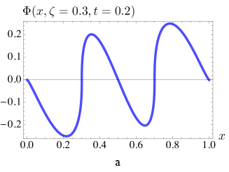
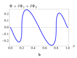
Figure 9: a) $\Phi(x,\zeta,t)$. b) $\Phi(x,\zeta,t)$ and $\delta\Psi_{1}(x,\zeta,t)+\delta\Psi_{2}(x,\zeta,t)$ ($\zeta=0.2$ and $t=0.2$).

V Evolution of cusp part of two-photon GDA

V.1 Decomposition

In this section, we study evolution of the second function, namely $\varphi_{2}(x,\zeta)$. Its initial form $\Phi_{2,0}(x,\zeta)$ is continuous for $x=\zeta$ and $x=\bar{\zeta}$ and is given by

$$\Phi_{2,0}(x,\zeta)= -\left(\frac{x}{\zeta}\right)\,\frac{1+\zeta-4\zeta^{2}+4(\zeta-x)}{2(1-\zeta)}\,\theta(x<\zeta)-\{x\to 1-x\}-\left(\frac{1-2x}{1-2\zeta}\right)\frac{1+\zeta-4\zeta^{2}}{2(1-{\zeta})}\,\theta(\zeta<x<\bar{\zeta})\ ,$$ (57)

see Fig.10a. We can separate this function

$$\Phi_{2,0}(x,\zeta)= -\frac{1+\zeta-4\zeta^{2}}{2(1-\zeta)}\Phi^{\text{L}}_{2,0}(x,\zeta)+\Phi^{\text{C}}_{2,0}(x,\zeta)$$ (58)

into a term proportional to a linearized function, Fig.10b,

$$\Phi^{\text{L}}_{2,0}(x,\zeta)= \frac{x}{\zeta}\,\theta(x<\zeta)-\{x\to 1-x\}-\left(\frac{1-2x}{1-2\zeta}\right)\theta(\zeta<x<\bar{\zeta})\ ,$$ (59)

and the remaining curvy part (see Fig.11a below),

$$\Phi^{\text{C}}_{2,0}(x,\zeta)= \frac{2x(x-\zeta)}{\zeta\bar{\zeta}}\,\theta(x<\zeta)-\{x\to 1-x\}\ .$$ (60)

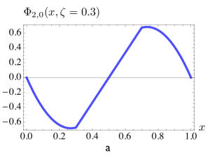
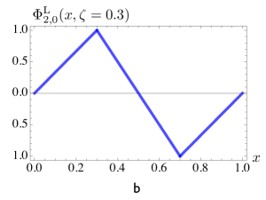
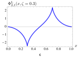
Figure 10: a) Initial function $\Phi_{2,0}(x,\zeta)$ for $\zeta=0.3$. b) Initial form $\Phi^{L}_{2,0}(x,\zeta=0.3)$ of the linearized part. c) First iteration function $\Phi^{L}_{2,1}(x,\zeta=0.3)$ for the linearized part.

V.2 Evolution of linearized part

Since $\Phi_{2,0}(x,\zeta)$ is a continuous function vanishing at the end points, the easiest way to get its evolution is to use straightforward $t^{n}$ expansion with coefficients given by successive iterations of the evolution kernel with $\Phi_{2,0}(x,\zeta)$. The first iteration of $\Phi^{\text{L}}_{2,0}(x,\zeta)$ gives

$$\Phi^{\text{L}}_{2,1}(x,\zeta)= -\frac{\theta(0<x<\zeta)}{\zeta(1-2\zeta)}\biggl{\{}+{\bar{x}}\Bigl{[}\bar{\zeta}\ln\bar{\zeta}-\zeta\ln\zeta\Bigr{]}+(1-2\zeta)\Bigl{[}x+x\bar{x}\ln x+(1-x\bar{x})\ln\bar{x}\Bigr{]}$$

$$+(\zeta-x)\ln(\zeta-x)-(\bar{\zeta}-x)\ln(\bar{\zeta}-x)\biggr{\}}-\{x\rightarrow\bar{x}\}$$

$$-\frac{\theta(\zeta<x<\bar{\zeta})}{1-2\zeta}\biggl{\{}(1-2x)\Bigl{[}1+\frac{\bar{\zeta}}{\zeta}\,\ln\bar{\zeta}\Bigr{]}+2x\bar{x}\ln\frac{\bar{x}}{x}+\left(\frac{x}{\zeta}-1\right)\ln\left(1-\frac{\zeta}{x}\right)-\left(\frac{\bar{x}}{\zeta}-1\right)\ln\left(1-\frac{\zeta}{\bar{x}}\right)\biggr{\}}$$

$$+v(x)\Phi^{\text{L}}_{2,0}(x,\zeta)\,.$$ (61)

Here, as usual, $v(x)$ is $3/2+x\ln\bar{x}+\bar{x}\ln x$. The structure of the result is very similar to that of $\Phi_{2,1}(x,\zeta)$. However, the potentially singular logarithmic terms $\ln|x-\zeta|$ and $\ln|x-\bar{\zeta}|$ are accompanied in this case by $(x-\zeta)$ or $(x-\bar{\zeta})$ factors, respectively, and vanish at these points, though having singular derivatives there. Thus, the function $\Phi_{2,1}(x,\zeta)$, shown in Fig. 10c, is continuous at points $x=\zeta$ and $x=\bar{\zeta}$.

V.3 Evolution of curvy part and total result

Initially, the support region for the curvy part $\Phi^{\text{C}}_{2,0}(x,\zeta)$ is restricted by two segments $0<x<\zeta$ and $\bar{\zeta}<x<1$, see Fig.11a.

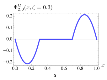
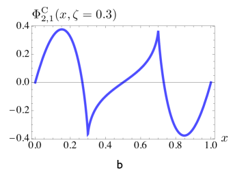
Figure 11: Initial form $\Phi^{\text{C}}_{2,0}(x,\zeta=0.2)$ for curvy part (a) and its first iteration (b).

Its first iteration is given by

$$\Phi^{\text{C}}_{2,1}= -\frac{\theta(0<x<\zeta)}{\zeta\bar{\zeta}}\biggl{\{}x[3x-4\zeta+2\zeta^{2}]+2[x\bar{x}(3+x-\zeta)+\bar{\zeta}]\ln\bar{x}-2\bar{x}\bar{\zeta}\,\ln\bar{\zeta}+2x\bar{x}(x-\zeta)\ln x$$

$$+2x(\zeta-x)\ln(\zeta-x)-2\bar{x}(\bar{\zeta}-x)\ln(\bar{\zeta}-x)\biggr{\}}-\{x\rightarrow\bar{x}\}$$

$$-\frac{\theta(\zeta<x<\bar{\zeta})}{\zeta\bar{\zeta}}\biggl{\{}-(1-2x)\zeta^{2}-2x(x-\zeta)\ln x+2\bar{x}(\bar{\zeta}-x)\ln\bar{x}+2(1-2x)\bar{\zeta}\ln\bar{\zeta}$$

$$+2x(x-\zeta)\ln(x-\zeta)-2\bar{x}(\bar{\zeta}-x)\ln(\bar{\zeta}-x)\biggr{\}}+v(x)\Phi^{\text{L}}_{2,0}(x,\zeta)\,.$$ (62)

One can see from Fig. 11b that evolution spreads the function into to the $\zeta<x<\bar{\zeta}$ interval. Combining the results for the linearized and curvy parts, we arrive at the evolution pattern generated for $\varphi_{2}(x,\zeta;t)$ by the first iteration (see Fig. 12a).

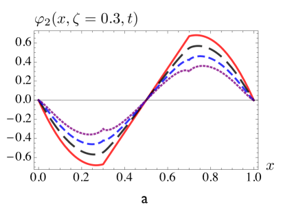
Figure 12: Evolution of $\phi_{2}(x,\zeta,t)$ at $t=0$, $t=0.2$, $t=0.3$ and $t=0.5$. Evolution of total GDA $\Phi(x,\zeta,t)$ at $t=0$, $t=0.1$, $t=0.2$ and $t=0.3$

Adding the result for $\varphi_{1}(x,\zeta,t)$ obtained in previous sections, we end up with the evolution of the total function $\varphi(x,\zeta,t)$ illustrated in Fig. 12b.

VI Summary

In this paper, we described a new method for performing analytic ERBL evolution for distribution amplitudes. Our approach is very efficient in application to functions that do not vanish at the end points or have jumps and cusps inside the support region $0<x<1$. Unlike the standard method of expansion in Gegenbauer polynomials, which requires an infinite number of terms in order to eliminate singularities of initial distributions, our method needs only one or two iterations in order to get a reliable and continuous result. The method was illustrated for two cases of the initial DA: for a purely flat DA, constant in the whole $0\leq x\leq 1$ interval and for an antisymmetric DA which is constant in each of its two parts $0\leq x\leq 1/2$ and $1/2\leq x\leq 1$. In case of a purely flat DA, the leading term gives $(x\bar{x})^{t}$ evolution with the change of the evolution parameter $t$. For the accompanying factor, two further terms in the $t^{N}$ expansion were found. In case of an antisymmetric flat DA, there is an extra factor $|1-2x|^{2t}$ that takes care of the jump in the middle point $x=1/2$. The correction terms were also calculated. The results show good convergence for $t\lesssim 1/2$. It should be noted that for $t\gtrsim 1/2$, the evolved DA is rather close to the asymptotic form, and one can use the standard method of the Gegenbauer expansion which is well convergent for such functions. The method was also applied for studying the evolution of the (logarithmic $Q^{2}$ derivative) of the two-photon GDA.

The methods developed in the present paper, may be extended onto application to generalized parton distributions. In that case, two strategies are possible. The first strategy is to use a direct evolution equation for GPD $H(x,\xi;t)$. In that case, both the GPD and the evolution kernel depend on the skewness parameter $\xi$, which is analogous to the parameter $\zeta$ encountered in the two-photon GDA studies. Another strategy is to use the evolution equation for the double distribution $F(\beta,\alpha;t)$. In this case, no skewness parameter is present in the evolution equation, and dependence on $\xi$ appears after one performs the conversion of the double distribution into a GPD. In both cases, various aspects of our methods of analytic evolution may be used. In particular, GPDs are non-analytic at the border points $x=\pm\xi$, having there cusps, while model DDs may have a singular structure (jumps, delta-functions) present in their initial shape.

References

- Mueller et al. (1994) D. Mueller, D. Robaschik, B. Geyer, F. M. Dittes, and J. Horejsi, Fortschr. Phys., 42, 101 (1994), arXiv:hep-ph/9812448 .
- Ji (1997) X.-D. Ji, Phys. Rev. Lett., 78, 610 (1997), arXiv:hep-ph/9603249 .
- Radyushkin (1996) A. V. Radyushkin, Phys. Lett., B380, 417 (1996), arXiv:hep-ph/9604317 .
- Collins et al. (1997) J. C. Collins, L. Frankfurt, and M. Strikman, Phys. Rev., D56, 2982 (1997), arXiv:hep-ph/9611433 .
- Ji (1998) X.-D. Ji, J. Phys., G24, 1181 (1998), arXiv:hep-ph/9807358 .
- Martin and Ryskin (1998) A. D. Martin and M. G. Ryskin, Phys. Rev., D57, 6692 (1998), arXiv:hep-ph/9711371 .
- Pire et al. (1999) B. Pire, J. Soffer, and O. Teryaev, Eur. Phys. J., C8, 103 (1999), arXiv:hep-ph/9804284 .
- Radyushkin (1999) A. V. Radyushkin, Phys. Rev., D59, 014030 (1999), arXiv:hep-ph/9805342 .
- Tandogan and Radyushkin (2011) A. Tandogan and A. V. Radyushkin, Int.J.Mod.Phys. Conf.Ser., 04, 227 (2011), arXiv:1109.2531 [hep-ph] .
- Diehl et al. (1998) M. Diehl, T. Gousset, B. Pire, and O. Teryaev, Phys.Rev.Lett., 81, 1782 (1998), arXiv:hep-ph/9805380 [hep-ph] .
- Tandogan and Radyushkin (2014) A. Tandogan and A. V. Radyushkin, Int.J.Mod.Phys. Conf.Ser., 25, 1460037 (2014).
- Efremov and Radyushkin (1980) A. Efremov and A. Radyushkin, Phys.Lett., B94, 245 (1980).
- Lepage and Brodsky (1980) G. P. Lepage and S. J. Brodsky, Phys.Rev., D22, 2157 (1980).
- Pire and Szymanowski (2003) B. Pire and L. Szymanowski, Phys.Lett., B556, 129 (2003), arXiv:hep-ph/0212296 [hep-ph] .
- El Beiyad et al. (2008) M. El Beiyad, B. Pire, L. Szymanowski, and S. Wallon, Phys.Rev., D78, 034009 (2008), arXiv:0806.1098 [hep-ph] .