Detrended Structure-Function in Fully Developed Turbulence

Abstract

The classical structure-function (SF) method in fully developed turbulence or for scaling processes in general is influenced by large-scale energetic structures, known as infrared effect. Therefore, the extracted scaling exponents $\zeta(n)$ might be biased due to this effect. In this paper, a detrended structure-function (DSF) method is proposed to extract scaling exponents by constraining the influence of large-scale structures. This is accomplished by removing a $1$st-order polynomial fitting within a window size $\ell$ before calculating the velocity increment. By doing so, the scales larger than $\ell$, i.e., $r\geq\ell$, are expected to be removed or constrained. The detrending process is equivalent to be a high-pass filter in physical domain. Meanwhile the intermittency nature is retained. We first validate the DSF method by using a synthesized fractional Brownian motion for mono-fractal processes and a lognormal process for multifractal random walk processes. The numerical results show comparable scaling exponents $\zeta(n)$ and singularity spectra $D(h)$ for the original SFs and DSFs. When applying the DSF to a turbulent velocity obtained from a high Reynolds number wind tunnel experiment with $Re_{\lambda}\simeq 720$, the 3rd-order DSF demonstrates a clear inertial range with $\mathcal{B}_{3}(\ell)\simeq 4/5\epsilon\ell$ on the range $10<\ell/\eta<1000$, corresponding to a wavenumber range $0.001<k\eta<0.1$. This inertial range is consistent with the one predicted by the Fourier power spectrum. The directly measured scaling exponents $\zeta(n)$ (resp. singularity spectrum $D(h)$) agree very well with a lognormal model with an intermittent parameter $\mu=0.33$. Due to large-scale effects, the results provided by the SFs are biased. The method proposed here is general and can be applied to different dynamics systems in which the concepts of multiscale and multifractal are relevant.

1 Introduction

Multiscale dynamics is present in many phenomena, e.g., turbulence [1], finance [2, 3], geosciences [4, 5], etc, to quote a few. It has been found in many multiscale dynamics systems that the self-similarity is broken, in which the concept of multiscaling or multifractal is relevant [1]. This is characterized conventionally by using the structure-functions (SFs), i.e., $S_{n}(\ell)=\langle\Delta u_{\ell}(x)^{n}\rangle\sim\ell^{\zeta(n)}$, in which $\Delta u_{\ell}(x)=u(x+\ell)-u(x)$ is an increment with separation scale $\ell$. Note that for the self-similarity process, e.g., fractional Brownian motion (fBm), the measured $\zeta(n)$ is linear with $n$. While for the multifractal process, e.g., turbulent velocity, it is usually convex with $n$. Other methods are available to extract the scaling exponent. For example, wavelet based methodologies, (e.g., wavelet leaders, wavelet transform modulus maxima [6, 7, 5]), Hilbert-based method [8, 9], or the scaling analysis of probability density function of velocity increments [10], to name a few. Each method has its owner advantages and shortcomings. For example, the classical SFs is found to mix information of the large- (resp. known as infrared effect) and small-scale (resp. known as ultraviolet effect) structures [11, 12, 13, 9, 14]. The corresponding scaling exponent $\zeta(n)$ is thus biased when a large energetic structure is present [9].

Previously the influence of the large-scale structure has been considered extensively by several authors [15, 16, 17, 12, 13, 18]. For example, Praskvosky et al., [15] found strong correlations between the large scales and the velocity SFs at all length scales. Sreenivasan & Stolovitzky Sreenivasan1996PRL [16] observed that the inertial range of the SFs conditioned on the large scale velocity show a strong dependence. Huang et al., Huang2010PRE [12] showed analytically that the influence of the large-scale structure could be as large as two decades down to the small scales. Blum et al., Blum2010PoF [13] studied experimentally the nonuniversal large-scale structure by considering both conditional Eulerian and Lagrangian SFs. They found that both SFs depend on the strength of large-scale structures at all scales. In their study, the large-scale structure velocity is defined as two-point average, i.e., $\sum u_{z}(\ell)=[u_{z}(x)+u_{z}(x+\ell)]/2$, in which $u_{z}$ is the vertical velocity in their experiment apparatus. Note that they conditioned SFs on different intensity of $\sum u_{z}(\ell)$. Later, Blum et al., Blum2011NJP [18] investigated systematically the large-scale structure conditioned SFs for various turbulent flows. They confirmed that in different turbulent flows the conditioned SFs depends strongly on large-scale structures at all scales.

In this paper, a detrended structure-function (DSF) method is proposed to extract scaling exponents $\zeta(n)$. This is accomplished by removing a $1$st-order polynomial within a window size $\ell$ before calculating the velocity increment. This procedure is designated as detrending analysis (DA). By doing so, scales larger than $\ell$, i.e., $r\geq\ell$, are expected to be removed or constrained. Hence, the DA acts as a high-pass filter in physical domain. Meanwhile, the intermittency is still retained. A velocity increment $\Delta u_{i,\ell}(x)$ is then defined within the window size $\ell$. A $n$th-order moment of $\Delta u_{i,\ell}(x)$ is introduced as $n$th-order DSF. The DSF is first validated by using a synthesized fractional Brownian motion (fBm) and a lognormal process with an intermittent parameter $\mu=0.15$ respectively for mono-fractal and multifractal processes. It is found that DSFs provide comparable scaling exponents $\zeta(n)$ and singularity spectra $D(h)$ with the ones provided by the original SFs. When applying to a turbulent velocity with a Reynolds number $Re_{\lambda}=720$, the $3$rd-order DSF shows a clear inertial range $10<\ell/\eta<1000$, which is consistent with the one predicted by the Fourier power spectrum $E_{u}(k)$, e.g., $0.001<k\eta<0.1$. Moreover, a compensated height of the $3$rd-order DSF is $0.80\pm 0.05$. This value is consistent with the famous Kolmogorov four-fifth law. The directly measured scaling exponents $\zeta(n)$ (resp. singularity spectrum $D(h)$) agree very well with the lognormal model with an intermittent parameter $\mu=0.33$. Due to the large-scale effect, known as infrared effect, the SFs are biased. Note that the scaling exponents are extracted directly without resorting to the Extended-Self-Similarity (ESS) technique. The method is general and could be applied to different types of data, in which the multiscale and multifractal concepts are relevant.

2 Detrending Analysis and Detrended Structure-Function

2.1 Detrending Analysis

We start here with a scaling process $u(x)$, which has a power-law Fourier spectrum, i.e.,

$$E(k)=Ck^{-\beta}$$ (1)

in which $\beta$ is the scaling exponent of $E(k)$. The Parseval’s theorem states the following relation, i.e.,

$$\langle u(x)^{2}\rangle_{x}=\int_{0}^{+\infty}E(k)\mathrm{\,d}k$$ (2)

in which $\langle\,\rangle$ is ensemble average, $E(k)$ is the Fourier power spectrum of $u(x)$ [19]. We first divide the given $u(x)$ into $m$ segments with a length $\ell$ each. A $q$th-order detrending of the $i$th segment is defined as, i.e.,

$$u_{i,\ell}(x)=u_{i}(x)-P_{i,\ell}^{q}(x),\,(i-1)\ell\leq x\leq i\ell$$ (3)

in which $P_{i,\ell}^{q}(x)$ is a $q$th-order polynomial fitting of the $u_{i}(x)$. We consider below only for the first-order detrending, i.e., $q=1$. To obtain a detrended signal, i.e., $u_{\ell}(x)=[u_{1,\ell}(x),u_{2,\ell}(x)\cdots u_{m,\ell}(x)]$, a linear trend is removed within a window size $\ell$. Ideally, scales larger than $\ell$, i.e., $r>\ell$ are removed or constrained from the original data $u(x)$. This implies that the DA procedure is a high-pass filter in the physical domain. The kinetic energy of $u_{\ell}(x)$ is related directly with its Fourier power spectrum, i.e.,

$$\mathcal{D}_{2}(\ell)=\langle u_{\ell}(x)^{2}\rangle_{x}=\int_{0}^{+\infty}E_{\ell}(k)\mathrm{\,d}k\simeq\int_{k_{\ell}}^{+\infty}E(k)\mathrm{\,d}k$$ (4)

in which $k_{\ell}=1/\ell$ and $E_{\ell}(k)$ is the Fourier power spectrum of $u_{\ell}(x)$. This illustrates again that the DA procedure acts a high-pass filter, in which the lower Fourier modes $k<k_{\ell}$ (resp. $r>\ell$) are expected to be removed or constrained. For a scaling process, i.e., $E(k)\sim k^{-\beta}$, it leads a power-law behavior, i.e.,

$$\mathcal{D}_{2}(\ell)\sim k_{\ell}^{1-\beta}\sim\ell^{\beta-1}$$ (5)

The physical meaning of $\mathcal{D}_{2}(\ell)$ is quite clear. It represents a cumulative energy over the Fourier wavenumber band $[k_{\ell},+\infty]$ (resp. scale range $[0,\ell]$). We emphasize here again that the DA acts as a high-pass filter in physical domain and the intermittency nature of $u(x)$ is still retained.

2.2 Detrended Structure-Function

The above mentioned detrending analysis can remove/constrain the large-scale influence, known as infrared effect. This could be utilized to redefine the SF to remove/constrain the large-scale structure effect as following. After the DA procedure, , the velocity increment can be defined within a window size $\ell$ as, i.e.,

$$\Delta u_{i,\ell}(x)=u_{i,\ell}(x+\ell/2)-u_{i,\ell}(x)$$ (6)

in which $i$ represents for the $i$th segment. We will show in the next subsection why we define an increment with a half width of the window size. A $n$th-order DSF is then defined as, i.e.,

$$\mathcal{B}_{n}(\ell)=\langle\Delta u_{i,\ell}(x)^{n}\rangle_{x}$$ (7)

For a scaling process, we expect a power-law behavior, i.e.,

$$\mathcal{B}_{n}(\ell)\sim\ell^{\zeta(n)}$$ (8)

in which the scaling exponent $\zeta(n)$ is comparable with the one provided by the original SFs.

To access negative orders of $n$ (resp. the right part of the singularity spectrum $D(h)$, see definition below), the DSFs can be redefined as, i.e.,

$$\mathcal{B}_{n}(\ell)=\langle X_{\ell}(i)^{n}\rangle$$ (9)

in which $X_{\ell}(i)=\langle|\Delta u_{i,\ell}(x)|\rangle_{(i-1)\ell\leq x\leq i\ell}$ is local average for the $i$th segment. A power-law behavior is expected, i.e., $\mathcal{B}_{n}(\ell)\sim\ell^{\zeta(n)}$. It is found experimentally that when $q>0$, Eqs. (7) and  (9) provide the same scaling exponents $\zeta(n)$. In the following we do not discriminate these two definitions for DSFs.

2.3 An Interpretation in Time-wavenumber Analysis Frame

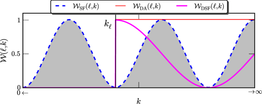
Figure 1: (Color online) An illustration of the weight function $\mathcal{W}(\ell,k)$ for different methods: structure-function $\mathcal{W}_{\textrm{SF}}=1-\cos(2\pi k\ell)$ (dashed line), first-order detrending analysis $\mathcal{W}_{\mathrm{DA}}$ (thin solid line), and the detrended structure-function $\mathcal{W}_{\mathrm{DSF}}$ (thick solid line). The detrended scale $\ell$ is demonstrated by a vertical solid line with $k_{\ell}=1/\ell$. Ideally, scales larger than $\ell$, i.e., $r<\ell$ (resp. $k<k_{\ell}$) are expected to be removed after the detrending process.

To understand better the filter property of the detrending procedure and DSFs, we introduce here a weight function $\mathcal{W}(\ell,k)$, i.e.,

$$M_{2}(\ell)=\int_{0}^{+\infty}\mathcal{W}(\ell,k)E(k)\mathrm{\,d}k$$ (10)

in which $E(k)$ is the Fourier power spectrum of $u(x)$, and $M_{2}(\ell)$ is a second-order moment, which could be one of $\mathcal{D}_{2}(\ell)$ or $\mathcal{B}_{2}(\ell)$, or $S_{2}(\ell)$, respectively. The weight function $\mathcal{W}(\ell,k)$ characterizes the contribution of the Fourier component to the corresponding second-order moment. Note that an integral constant is neglected in the eq. (10). For the second-order SFs, one has the following weight function [1, 12], i.e.,

$$\mathcal{W}_{\mathrm{SF}}(\ell,k)=1-\cos\left(2\pi k\ell\right)$$ (11)

For a scaling process, one usually has a fast decaying Fourier spectrum, i.e. $E(k)\sim k^{-\beta}$ with $\beta>0$. Hence, the contribution from small-scale (resp. high wavenumber Fourier mode) is decreasing. The SFs might be more influenced by the large-scale part for large values of $\beta$ [12, 14, 20]. For the detrended data, the corresponding weight function is ideally to be as the following, i.e.,

$$\mathcal{W}_{\mathrm{DA}}(\ell,k)=\left\{\begin{array}[]{lll}&0,&\textrm{when $k\leq k_{\ell}$}\\ &1,&\textrm{when $k>k_{\ell}$ }\end{array}\right.$$ (12)

The DSFs (resp. the combination of the DA and SF) have a weight function, i.e.,

$$\mathcal{W}_{\mathrm{DSF}}(\ell,k)=\left\{\begin{array}[]{lll}&0,&\textrm{when $k\leq k_{\ell}$}\\ &1-\cos\left(\pi k\ell\right),&\textrm{when $k>k_{\ell}$ }\end{array}\right.$$ (13)

Comparing with the original SFs, the DSFs defined here can remove/constrain the large-scale effect. Figure 1 shows the corresponding $\mathcal{W}(\ell,k)$ for the SF, detrending analysis, and DSF, respectively. The detrended scale $\ell$ is illustrated by a vertical line, i.e., $k_{\ell}=1/\ell$. We note here that with the definition of Eq. (6), $\mathcal{B}_{2}(\ell)$ provides a better compatible interpretation with the Fourier power spectrum $E(k)$ since we have $\mathcal{W}_{\mathrm{DSF}}(\ell,k_{\ell})=1$. This is the main reason why we define the velocity increment with the half size of the window width $\ell$.

We provide some comments on Eq. (10). The above argument is exactly valid for linear and stationary processes. In reality, the data are always nonlinear and nonstationary for some reasons, see more discussion in Ref. [21]. Therefore, eq. (10) holds approximately for real data. Another comment has to be emphasized here for the detrending procedure. Several approaches might be applied to remove the trend [22, 23]. However, the trend might be linear or nonlinear. Therefore, different detrending approaches might provide different performances. In the present study, we only consider the $1$st-order polynomial detrending procedure, which is efficient for many types of data.

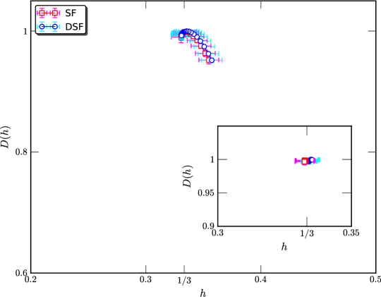
Figure 2: (Color online) Measured singularity spectrum $D(h)$ for fractional Brownian motion with $H=1/3$ on the range $-4\leq n\leq 4$. The inset shows the singularity spectrum $D(n)$ on the range $0\leq n\leq 4$. The errorbar is the standard deviation estimated from 100 realizations. Ideally, one should have $h=1/3$ and $D(1/3)=1$. Both methods provide the same $h$ and $D(h)$ and statistical error.

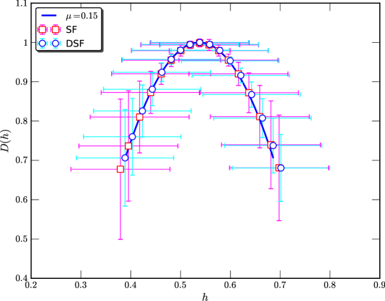
Figure 3: (Color online) Measured singularity spectrum $D(h)$ for the lognormal process with an intermittent parameter $\mu=0.15$. The errorbar is the standard deviation from the 100 realizations. The theoretical singularity curve is illustrated by a solid line. Both estimators provide the same singularity spectra $D(h)$ and statistical error.

3 Numerical Validation

3.1 Fractional Brownian Motion

We first consider here the fractional Brownian motion as a typical mono-scaling process. FBm is a Gaussian self-similar process with a normal distribution increment, which is characterized by $H$, namely Hurst number $0<H<1$ [24, 25, 26, 27]. A Wood-Chan algorithm is used to synthesize the fBm with a Hurst number $H=1/3$. We perform 100 realizations with a data length $10^{5}$ points each. Power-law behavior is observed on a large-range of scales for $-4\leq n\leq 4$. The corresponding singularity spectrum is, i.e.,

$$h=\zeta^{\prime}{}(n),\,D(h)=\min_{n}\{hn-\zeta(n)+1\}$$ (14)

Ideally, one should have a single point of singularity spectrum with $h=1/3$ and $D(1/3)=1$. However, in practice, the measured singularity spectrum $D(h)$ is always lying in a narrow band. Figure 2 shows the measured singularity spectrum $D(h)$ for SFs ($\square$) and DSFs ($\ocircle$) for $-4\leq n\leq 4$, in which the inset shows the singularity spectra $D(h)$ estimated on the range $0\leq n\leq 4$. Visually, both estimators provide the same $D(h)$ and the same statistical error, which is defined as the standard deviation from different realizations.

3.2 Multifractal Random Walk With a Lognormal Statistics

We now consider a multifractal random walk with a lognormal statistics [28, 29, 30]. A multiplicative discrete cascade process with a lognormal statistics is performed to simulate a multifractal measure $\epsilon(x)$. The larger scale corresponds to a unique cell of size $L=\ell_{0}\lambda_{1}^{N}$, where $\ell_{0}$ is the largest scale considered and $\lambda_{1}>1$ is a dimensional scale ratio. In practice for a discrete model, this ratio is often taken as $\lambda_{1}=2$ [30, 9]. The next scale involved corresponds to $\lambda_{1}$ cells, each of size $L/\lambda_{1}=\ell_{0}\lambda_{1}^{N-1}$. This is iterated and at step $p$ ($1\leq p\leq N$) $\lambda_{1}^{p}$ cells are retrieved. Finally, at each point the multifractal measure $\epsilon(x)$ is as the product of $n$ cascade random variables, i.e.,

$$\epsilon(x)=\prod_{m=1}^{N}W_{m}(x)$$ (15)

where $W_{m}(x)$ is the random variable corresponding to position $x$ and level $m$ in the cascade [30]. Following the multifractal random walk idea [28, 29], a nonstationary multifractal time series can be synthesized as, i.e.,

$$u(x)=\int_{0}^{x}{\epsilon(x^{\prime})^{1/2}}\mathrm{\,d}B(x^{\prime})$$ (16)

where $B(x)$ is Brownian motion. Taking a lognormal statistic for $\epsilon$, the scaling exponent $\zeta(n)$ for the SFs, i.e., $\langle\Delta u_{\ell}(x)^{n}\rangle\sim\ell^{\zeta(n)}$, is written as,

$$\zeta(n)=\frac{n}{2}-\frac{\mu}{2}(\frac{n^{2}}{4}-\frac{n}{2})$$ (17)

where $\mu$ is the intermittency parameter ($0\leq\mu\leq 1$) characterizing the lognormal multifractal cascade [30].

Synthetic multifractal time series are generated following Eq. (16). An intermittent parameter $\mu=0.15$ is chosen for $m=17$ levels each, corresponding to a data length $131072$ points each. A total of 100 realizations are performed. The statistical error is then measured as the standard deviation from these realizations. Figure 3 shows the corresponding measured singularity spectra $D(h)$, in which the theoretical value is illustrated by a solid line. Graphically, the theoretical singularity spectra $D(h)$ are recovered by both estimators. Statistical error are again found to be the same for both estimators.

We would like to provide some comments on the performance of these two estimators. For the synthesized processes, they have the same performance since there is no intrinsic structure in these synthesized data. But for the real data, as we mentioned above, they possess nonstationary and nonlinear structures [21]. Therefore, as shown in below, they might have different performance.

4 Application to Turbulent Velocity

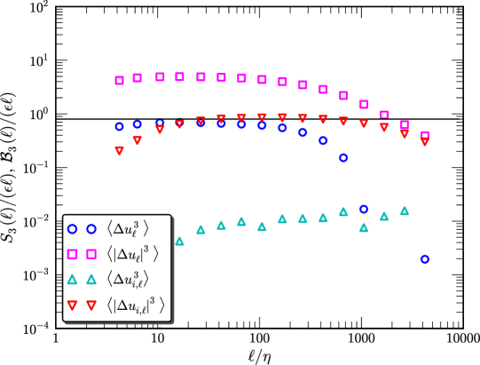
Figure 4: (Color online) Measured compensated 3rd-order moments $S_{3}(\ell)/(\epsilon\ell)$ and $\mathcal{B}_{3}(\ell)/(\epsilon\ell)$ from experimental homogeneous and nearly isotropic turbulent flow. They are respectively 3rd-order SFs with ($\square$) and without ($\ocircle$) absolute value, and 3rd-order DSFs with ($\triangledown$) and without ($\triangle$) absolute value. The horizontal solid line indicates the Kolmogorov’s four-fifth law. An observed plateau for $\mathcal{B}_{3}(\ell)/{\epsilon\ell}$ indicates an inertial range on the range $10<\ell/\eta<1000$, corresponding to a wavenumber range $0.001<k\eta<0.1$. Roughly speaking, a plateau for $S_{3}(\ell)/{\epsilon\ell}$ indicates an inertial range on the range $10<\ell/\eta<100$. The height of the inertial range are respectively $0.67\pm 0.02$ ($\ocircle$), $4.84\pm 0.14$ ($\square$), $0.0098\pm 0.0024$ ($\triangle$) and $0.80\pm 0.05$ ($\triangledown$), in which the statistical error is the standard deviation obtained from the inertial range. Note that the inertial range are $10<\ell/\eta<100$ for the SFs and $10<\ell/\eta<1000$ for the DSFs. The corresponding scaling exponents $\zeta(3)$ are $0.95\pm 0.02$, $0.84\pm 0.03$, $1.15\pm 0.07$ and $0.99\pm 0.03$. The statistical error is the 95% fitting confidence on the inertial range.

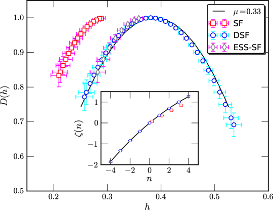
Figure 5: (Color online) Measured singularity spectrum $D(h)$. The errorbar is the standard deviation from 120 realizations. The inset shows the corresponding scaling exponents $\zeta(n)$. For comparison, the lognormal model with an intermittent parameter $\mu=0.33$ is illustrated by a solid line.

We consider here a velocity database obtained from a high Reynolds number wind tunnel experiment in the Johns-Hopkins university with Reynolds number $Re_{\lambda}=720$. An probe array with four X-type hot wire anemometry is used to record the velocity with a sampling wavenumber of $40$ kHz at streamwise direction $x/M=20$, in which $M$ is the size of the active grid. These probes are placed in the middle height and along the center line of the wind tunnel to record the turbulent velocity simultaneously for a duration of 30 second. The measurement is then repeated for 30 times. Finally, we have $30\times 4\times 30\times(4\times 10^{4})$ data points (number of measurements $\times$ number of probes $\times$ duration time $\times$ sampling wavenumber). Therefore, there are 120 realizations (number of measurements $\times$ number of probes). The Fourier power spectrum $E_{u}(k)$ of the longitudinal velocity reveals a nearly two decades inertial range on the wavenumber range $0.001<k\eta<0.1$ with a scaling exponent $\beta\simeq 1.65\pm 0.02$, see Ref. [31]. This corresponds to time scales $10<\ell/\eta<1000$. Here $\eta$ is the Kolmogorov scale. Note that we convert our results into spatial space by applying the Taylor’s frozen hypothesis [1]. More detail about this database can be found in Ref. [31].

To determine the inertial range in real space, we plot the measured compensated 3rd-order moments in Fig.4 for the SFs ($S_{3}(\ell)/(\epsilon\ell)$ with ($\square$) and without ($\ocircle$) absolute value), DSFs ($\mathcal{B}_{3}(\ell)/(\epsilon\ell)$ with ($\triangledown$) and without ($\triangle$) absolute value), respectively. A horizontal solid line indicates the Kolmogorov’s four-fifth law. A plateau is observed for $\mathcal{B}_{3}(\ell)/(\epsilon\ell)$ on the range $10<\ell/\eta<1000$, which agrees very well with the inertial range predicted by $E_{u}(k)$, i.e., on the range $0.001<k\eta<0.1$. The corresponding height and scaling exponent are $0.80\pm 0.05$ with absolute value (resp. $0.0098\pm 0.0024$ without absolute value) and $\zeta(3)=0.99\pm 0.03$ (resp. $\zeta(3)=1.15\pm 0.07$), respectively. The statistical error is the standard deviation obtained from the range $10<\ell/\eta<1000$. Note that the Kolmogorov’s four-fifth law indicates a linear relation $\langle\Delta u_{\ell}^{3}\rangle=-4/5\epsilon\ell$. It is interesting to note that, despite of the sign, we have $\langle|\Delta u_{i,\ell}|^{3}\rangle=4/5\epsilon\ell$ on nearly two-decade scales. For comparison, the 3rd-order SFs are also shown. Roughly speaking, a plateau is observed on the range $10<\ell/\eta<100$. This inertial range is shorter than the one predicted by the Fourier analysis or DSFs, which is now understood as the large-scale influence. The corresponding height and scaling exponent are $0.67\pm 0.02$ without absolute value (resp. $4.84\pm 0.14$ with absolute value) and $0.95\pm 0.02$ (resp. $0.84\pm 0.03$). Therefore, the DSFs provide a better indicator of the inertial range since it removes/constrains the large-scale influence. We therefore estimate the scaling exponents for the $\mathcal{B}_{n}(\ell)$ on the range $10<\ell/\eta<1000$ for $-4\leq n\leq 4$ directly without resorting to the Extended Self-Similarity technique [32, 33]. For the SFs, we calculate the scaling exponents $\zeta(n)$ on the range $10<\ell/\eta<100$ for $0\leq n\leq 4$ directly.

Figure 5 shows the measured singularity spectra $D(h)$ for $-4\leq n\leq 4$, in which the errorbar is a standard deviation from 120 realizations. The inset shows the corresponding scaling exponents $\zeta(n)$. For comparison, the lognormal model $\zeta(n)=n/3-\mu/18\left(n^{2}-3n\right)$ with an intermittent parameter $\mu=0.33$ is shown as a solid line. Visually, the DSFs curve fully recovers the lognormal curve not only on the left part (resp. $n\geq 0$) but also on the right part (resp. $n\leq 0$). Due to the large-scale contamination, the SFs underestimates the scaling exponents $\zeta(n)$ when $n\geq 0$ [11, 12]. This leads an overestimation of the left part of singularity spectrum $D(h)$ (see $\square$ in Fig.5). However, if one resorts the ESS algorithm when measuring the SF scaling exponent $\zeta(n)$, the corresponding singularity spectrum $D(h)$ is then horizontal shifted to the theoretical curve. This has been interpreted as that the ESS technique suppresses the finite Reynolds number effect. We show here that if one removes/constrains the effect of large-scale motions, one can retrieve the scaling exponent $\zeta(n)$ (resp. singularity spectrum $D(h)$) without resorting the ESS technique. Or in other words, the finite Reynolds number effect manifests at large-scale motions, which is usually anisotropic too.

5 Conclusion

In this paper, we introduce a detrended structure-function analysis to remove/constrain the influence of large-scale motions, known as the infrared effect. In the first step of our proposal, the $1$st-order polynomial trend is removed within a window size $\ell$. By doing so, the scales larger than $\ell$, i.e., $r\geq\ell$, are expected to be removed/constrained. In the second step, a velocity increment is defined with a half of the window size. The DSF proposal is validated by the synthesized fractional Brownian motion for the mono-fractal process and a lognormal random walk for the multifractal process. The numerical test shows that both SFs and DSFs estimators provide a comparable performance for synthesized processes without intrinsic structures.

When applying to the turbulent velocity obtained from a high Reynolds number wind tunnel experiment, the 3rd-order DSFs show a clearly inertial range on the range $10<\ell/\eta<1000$ with a linear relation $\mathcal{B}_{3}(\ell)\simeq 4/5\epsilon\ell$. The inertial range provided by DSFs is consistent with the one predicted by the Fourier power spectrum. Note that, despite of the sign, the Kolmogorov’s four-fifth law is retrieved for the 3rd-order DSFs. The corresponding 3rd-order SFs are biased by the large-scale structures, known as the infrared effect. It shows a shorter inertial range and underestimate the 3rd-order scaling exponent $\zeta(3)$. The scaling exponents $\zeta(n)$ are then estimated directly without resorting to the ESS technique. The corresponding singularity spectrum $D(h)$ provided by the DSFs fully recovers the lognormal model with an intermittent parameter $\mu=0.33$ on the range $-4\leq n\leq 4$. However, the classical SFs overestimate the left part singularity spectrum $D(h)$ (resp. underestimate the corresponding scaling exponents $\zeta(n)$) on the range $0\leq n\leq 4$. This has been interpreted as finite Reynolds number effect and can be corrected by using the ESS technique. Here, to our knowledge, we show for the first time that if one removes/constrains the influence of the large-scale structures, one can recover the lognormal model without resorting to the ESS technique.

The method we proposed here is general and applicable to other complex dynamical systems, in which the multiscale statistics are relevant. It should be also applied systematically to more turbulent velocity databases with different Reynolds numbers to see whether the finite Reynolds number effect manifests on large-scale motions as well as we show for high Reynolds number turbulent flows.

References

- [1] U. Frisch Turbulence: the legacy of AN Kolmogorov, Cambridge University Press, 1995.
- [2] F. Schmitt, D. Schertzer, and S. Lovejoy, Multifractal fluctuations in finance, Int. J. Theor. Appl. Fin 3 (2000), pp. 361–364.
- [3] J. Muzy, D. Sornette, J. Delour, and A. Arneodo, Multifractal returns and hierarchical portfolio theory, Quant. Finance 1 (2001), pp. 131–148.
- [4] F. Schmitt, Y. Huang, Z. Lu, Y. Liu, and N. Fernandez, Analysis of velocity fluctuations and their intermittency properties in the surf zone using empirical mode decomposition, J. Mar. Sys. 77 (2009), pp. 473–481.
- [5] S. Lovejoy, and D. Schertzer, Haar wavelets, fluctuations and structure functions: convenient choices for geophysics, Nonlinear Proc. Geoph. 19 (2012), pp. 513–527.
- [6] B. Lashermes, S. Roux, P. Abry, and S. Jaffard, Comprehensive multifractal analysis of turbulent velocity using the wavelet leaders, Eur. Phys. J. B 61 (2008), pp. 201–215.
- [7] J. Muzy, E. Bacry, and A. Arneodo, Multifractal formalism for fractal signals: The structure-function approach versus the wavelet-transform modulus-maxima method, Phys. Rev. E 47 (1993), pp. 875–884.
- [8] Y. Huang, F. Schmitt, Z. Lu, and Y. Liu, An amplitude-frequency study of turbulent scaling intermittency using Hilbert spectral analysis, Europhys. Lett. 84 (2008), p. 40010.
- [9] Y. Huang, F.G. Schmitt, J.P. Hermand, Y. Gagne, Z. Lu, and Y. Liu, Arbitrary-order Hilbert spectral analysis for time series possessing scaling statistics: comparison study with detrended fluctuation analysis and wavelet leaders, Phys. Rev. E 84 (2011), p. 016208.
- [10] Y. Huang, F. Schmitt, Q. Zhou, X. Qiu, X. Shang, Z. Lu, and Y. Liu, Scaling of maximum probability density functions of velocity and temperature increments in turbulent systems, Phys. Fluids 23 (2011), p. 125101.
- [11] P.A. Davidson, and B.R. Pearson, Identifying turbulent energy distribution in real, rather than Fourier, space, Phys. Rev. Lett. 95 (2005), p. 214501.
- [12] Y. Huang, F. Schmitt, Z. Lu, P. Fougairolles, Y. Gagne, and Y. Liu, Second-order structure function in fully developed turbulence, Phys. Rev. E 82 (2010), p. 026319.
- [13] D.B. Blum, S.B. Kunwar, J. Johnson, and G.A. Voth, Effects of nonuniversal large scales on conditional structure functions in turbulence, Phys. Fluids 22 (2010), p. 015107.
- [14] Y. Huang, L. Biferale, E. Calzavarini, C. Sun, and F. Toschi, Lagrangian single particle turbulent statistics through the Hilbert-Huang Transforms, Phys. Rev. E 87 (2013), p. 041003(R).
- [15] A.A. Praskovsky, E.B. Gledzer, M.Y. Karyakin, and Y. Zhou, The sweeping decorrelation hypothesis and energy-inertial scale interaction in high Reynolds number flows, J. Fluid Mech. 248 (1993), p. 493.
- [16] K.R. Sreenivasan, and G. Stolovitzky, Statistical dependence of inertial range properties on large scales in a high-Reynolds-number shear flow, Phys. Rev. Lett. 77 (1996), p. 2218.
- [17] K.R. Sreenivasan, and B. Dhruva, Is there scaling in high-Reynolds number turbulence?, Prog. Theor. Phys. 130 (1998), pp. 103–120.
- [18] D.B. Blum, G.P. Bewley, E. Bodenschatz, M. Gibert, A. Gylfason, L. Mydlarski, G.A. Voth, H. Xu, and P. Yeung, Signatures of non-universal large scales in conditional structure functions from various turbulent flows, New J. Phys. 13 (2011), p. 113020.
- [19] D. Percival, and A. Walden Spectral Analysis for Physical Applications: Multitaper and Conventional Univariate Techniques, Cambridge University Press, 1993.
- [20] H. Tan, Y. Huang, and J.P. Meng, Hilbert Statistics of Vorticity Scaling in Two-Dimensional Turbulence, Phys. Fluids 26 (2014), p. 015106.
- [21] N. Huang, Z. Shen, S. Long, M. Wu, H. Shih, Q. Zheng, N. Yen, C. Tung, and H. Liu, The empirical mode decomposition and the Hilbert spectrum for nonlinear and non-stationary time series analysis, Proc. R. Soc. London, Ser. A 454 (1998), pp. 903–995.
- [22] Z. Wu, N.E. Huang, S.R. Long, and C. Peng, On the trend, detrending, and variability of nonlinear and nonstationary time series, PNAS 104 (2007), p. 14889.
- [23] A. Bashan, R. Bartsch, J. Kantelhardt, and S. Havlin, Comparison of detrending methods for fluctuation analysis, Physica A 387 (2008), pp. 5080–5090.
- [24] J. Beran Statistics for long-memory processes, CRC Press, 1994.
- [25] L. Rogers, Arbitrage with Fractional Brownian Motion, Math. Finance 7 (1997), pp. 95–105.
- [26] P. Doukhan, M. Taqqu, and G. Oppenheim Theory and Applications of Long-Range Dependence, Birkhauser, 2003.
- [27] C.W. Gardiner Handbook of Stochastic Methods, Springer, Berlin, third edition, 2004.
- [28] E. Bacry, J. Delour, and J. Muzy, Multifractal random walk, Phys. Rev. E 64 (2001).
- [29] J. Muzy, and E. Bacry, Multifractal stationary random measures and multifractal random walks with log infinitely divisible scaling laws, Phys. Rev. E 66 (2002), p. 056121.
- [30] F. Schmitt, A causal multifractal stochastic equation and its statistical properties, Eur. Phys. J. B 34 (2003), pp. 85–98.
- [31] H. Kang, S. Chester, and C. Meneveau, Decaying turbulence in an active-grid-generated flow and comparisons with large-eddy simulation, J. Fluid Mech. 480 (2003), pp. 129–160.
- [32] R. Benzi, S. Ciliberto, R. Tripiccione, C. Baudet, F. Massaioli, and S. Succi, Extended self-similarity in turbulent flows, Phys. Rev. E 48 (1993), pp. 29–32.
- [33] R. Benzi, S. Ciliberto, C. Baudet, G. Chavarria, and R. Tripiccione, Extended self-similarity in the dissipation range of fully developed turbulence, Europhys. Lett 24 (1993), pp. 275–279.