A hemispherical dynamo model : Implications for the Martian crustal magnetization

Abstract

Mars Global Surveyor measurements revealed that the Martian crust is strongly magnetized in the southern hemisphere while the northern hemisphere is virtually void of magnetization. Two possible reasons have been suggested for this dichotomy: A once more or less homogeneously magnetization may have been destroyed in the northern hemisphere by, for example, resurfacing or impacts. The alternative theory we further explore here assumes that the dynamo itself produced a hemispherical field (Stanley et al., 2008; Amit et al., 2011). We use numerical dynamo simulations to study under which conditions a spatial variation of the heat flux through the core-mantle boundary (CMB) may yield a strongly hemispherical surface field. We assume that the early Martian dynamo was exclusively driven by secular cooling and we mostly concentrate on a cosine CMB heat flux pattern with a minimum at the north pole, possibly caused by the impacts responsible for the northern lowlands. This pattern consistently triggers a convective mode which is dominated by equatorially anti-symmetric and axisymmetric (EAA, Landeau and Aubert (2011)) thermal winds. Convective up- and down-wellings and thus radial magnetic field production then tend to concentrate in the southern hemisphere which is still cooled efficiently while the northern hemisphere remains hot. The dynamo changes from an $\alpha^{2}$- for a homogeneous CMB heat flux to an $\alpha\Omega$-type in the hemispherical configuration. These dynamos reverse on time scales of about 10 kyrs. This too fast to allow for the more or less unidirectional magnetization of thick crustal layer required to explain the strong magnetization in the southern hemisphere.

1 Introduction

Starting in 1998 the space probe Mars Global Surveyor (MGS) delivered vector magnetic field data from orbits between $185$ and $400$ km above the planets surface (Acuña et al., 1999). The measurements reveal a strong but heterogeneous crustal magnetization (Acuña et al., 1999; Connerney et al., 2001). The more strongly magnetized rocks are mainly localized in the southern hemisphere where the crust is thick and old. The northern hemisphere is covered by a younger and thinner crust which is much weaker magnetized.

Two alternative types of scenarios are discussed to explain this dichotomy. One type explores the possibility that an originally more or less homogeneous magnetization was partly destroyed by resurfacing events after the demise of the internal dynamo. Based on the fact that the Hellas and Argyre impact basins are largely void of magnetization, Acuña et al. (2001) conclude that the dynamo stopped operating in the early Noachian before the related impact events happened roughly $3.7-4$ Gyrs ago. Volcanic activity and crustal spreading are two other possibilities to explain the lack of strong magnetization in certain surface areas (Lillis et al., 2008; Mohit and Arkani-Hamed, 2004), in particular the northern hemisphere after the dynamo cessation.

The alternative scenario explains the dichotomy by an ancient Martian dynamo that inherently produced a hemispherical magnetic field. Numerical dynamo simulations by Stanley et al. (2008) and Amit et al. (2011) show that this may happen when more heat is allowed to escape the core through the southern than through the northern core mantle boundary (CMB). Such north/south asymmetry can for example be caused by larger impacts or low-degree mantle convection (Roberts and Zhong, 2006; Keller and Tackley, 2009; Yoshida and Kageyama, 2006). Due to depth-dependent viscosity and a possible endothermic phase transition (Harder and Christensen, 1996) Martian mantle convection may be ruled in an extreme case by one gigantic plume typically evoked to explain the dominance of the volcanic Tharsis region. However, the single plume convection might have developed after the dynamo ceased. Due to the hotter temperature of the rising material the CMB heat flux can be significantly reduced under such a plume. Though Tharsis is roughly located in the equatorial region it could nevertheless lead to magnetic field with the observed north-south symmetry, as we will show in the following.

The possible effects of large impacts on planets and the dynamo in particular are little understood. Roberts et al. (2009) argue that impacts locally heat the underlying mantle and thereby lead to variations in the CMB heat flux. Large impacts may also cause a demise of the dynamo by reducing the CMB heat flux below the value where subcritical dynamo action is still possible (Roberts et al., 2009). The deposition of heat in the outer parts of the core by impact shock waves could lead to a stably stratified core and thereby also stop dynamo action (Arkani-Hamed and Olson, 2010) for millions of years until the heat has diffused out of the core. If the iron content of the impactor is large enough it may even trigger a dynamo (Reese and Solomatov, 2010).

The thermal state of the ancient Martian core is rather unconstrained (Breuer et al., 2010). Analysis of Martian meteorites suggests a significant sulphur content and thus a high core melting temperature (Dreibus and Wänke, 1985). Mars may therefore never have grown a solid inner core, an assumption we also adopt here (Schubert and Spohn, 1990; Breuer et al., 2010). The ancient Martian dynamo was then exclusively driven by secular cooling and radiogenic heating and has stopped operating when the CMB heat flux became subadiabatic (Stevenson et al., 1983). Run-away solidification or light element saturation may explain the dynamo cessation in the presence an inner core.

The geodynamo, on the other hand, is predominantly driven by the latent heat and light elements emanating from the growing inner core front. Secular cooling and radiogenic heating is typically modeled by homogeneously distributed internal buoyancy sources while the driving associated to inner core growth is modeled by bottom sources (Kutzner and Christensen, 2000). These latter sources have a higher Carnot efficiency and would likely have kept the Martian dynamo alive if the planet would have formed an inner core.

Several authors have explored the influence of a CMB heat flux pattern on dynamos geared to model Earth and report that they can cause hemispherical variations in the secular variation (Bloxham, 2000; Christensen and Olson, 2003; Amit and Olson, 2006), influence the reversal behavior (Glatzmaier et al., 1999; Kutzner and Christensen, 2004) or lead to inhomogeneous inner core growth (Aubert et al., 2008). However, the effects where never as drastic as those reported by Stanley et al. (2008) or Amit et al. (2011). In the work of Amit et al. (2011) the reason likely is the increased susceptibility of internally driven dynamos to the thermal CMB boundary condition (Hori et al., 2010). Stanley et al. (2008) retain bottom driving and employed a particularly strong heat flux variation to enforce a hemispherical field

Here, we follow Amit et al. (2011) in exploring the effects of a simple sinusoidal CMB heat flux variation on a dynamo model driven by internal heat sources. The main scope of this paper is to understand the particular dynamo mechanism, to explore its time dependence, and to extrapolate the results to the Martian situation. Section 2 introduces our model, whereas section 3 describes the effects of the CMB heat flux anomaly on the convection and the induction process. In section 4 we explore the applicability to the ancient Martian dynamo. The paper closes with a discussion in section 5.

2 Numerical Model

Using the MagIC code (Wicht, 2002; Christensen et al., 2007), we model the Martian core as a viscous, electrically conducting and incompressible fluid contained in a rotating spherical shell with inner core radius $r_{icb}$ and outer radius $r_{cmb}$. Conservation of momentum is described by the dimensionless Navier-Stokes equation for a Boussinesq fluid:

$$E\left(\frac{\partial\vec{u}}{\partial t}+\vec{u}\cdot\vec{\nabla}\vec{u}\right)=-\vec{\nabla}\Pi+E\nabla^{2}\vec{u}-2\hat{z}\times\vec{u}+\frac{RaE}{Pr}\frac{\vec{r}}{r_{cmb}}T+\frac{1}{Pm}(\vec{\nabla}\times\vec{B})\times\vec{B}\,$$ (1)

where $\vec{u}$ is the velocity field, $\Pi$ the generalized pressure, $\hat{z}$ the direction of the rotation axis, $T$ the super-adiabatic temperature and $\vec{B}$ the magnetic field.

The conservation of energy is given by

$$\frac{\partial T}{\partial t}+\vec{u}\cdot\vec{\nabla}T=\frac{1}{Pr}\nabla^{2}T+\epsilon\\ ,$$ (2)

where $\epsilon$ is a uniform heat source density. The conservation of magnetic field is given by the induction equation

$$\frac{\partial\vec{B}}{\partial t}=\vec{\nabla}\times\left(\vec{u}\times\vec{B}\right)+\frac{1}{Pm}\nabla^{2}\vec{B}\ .$$ (3)

We use the shell thickness $D=r_{cmb}-r_{icb}$ as length scale, the viscous diffusion time $D^{2}/\nu$ as time scale and $(\rho\mu\lambda\Omega)^{1/2}$ as the magnetic scale. The mean superadiabatic CMB heat flux density $q_{0}$ serves to define the temperature scale $q_{0}D/c_{p}\rho\kappa$. Here, $\nu$ is the viscous diffusivity, $\rho$ the constant background density, $\mu$ the magnetic permeability, $\lambda$ the magnetic diffusivity, $\Omega$ the rotation rate, $\kappa$ the thermal diffusivity and $c_{p}$ the heat capacity.

Three dimensionless parameters appear in the above system: the Ekman number $E=\nu/\Omega D^{2}$ is a measure for the relative importance of viscous versus Coriolis forces while the flux based Rayleigh number $Ra=\alpha g_{0}|q_{0}|D^{4}/\rho c_{p}\kappa^{2}\nu$ is a measure for the importance of buoyancy. The Prandtl number $P=\nu/\kappa$ and the magnetic Prandtl number $Pm=\nu/\lambda$ are diffusivity ratios.

An inner core with $r_{icb}/r_{cmb}=0.35$ is retained for numerical reasons (Hori et al., 2010), but to minimize its influence the heat flux from the inner core is set to zero. The secular cooling and radiogenic driving is modeled by the homogeneous heat sources $\epsilon$ appearing in 2 (Kutzner and Christensen, 2000). Furthermore we assume an electrically insulating inner core to avoid an additional sink for the magnetic field. We use no-slip, impermeable flow boundary conditions and match $\vec{B}$ to a potential field at the outer and inner boundary. The results by Hori et al. (2010) and Aubert et al. (2009) suggest that this is a fair approximation to model a dynamo without inner core since an additional reduction of the inner core radius has only a minor impact. The effective heat source $\epsilon$ is chosen to balance the mean heat flux $q_{0}$ through the outer boundary:

$$4\pi^{2}r_{cmb}^{2}\;q_{0} =-Pr\frac{4}{3}\pi(r_{cmb}^{3}-r_{icb}^{3})\;\epsilon\ .$$ (4)

Note that $q_{0}$ is generally negative. The CMB heat flux pattern is modeled in terms of spherical harmonic contributions with amplitude $q_{lm}$, where $l$ is the degree and $m$ the spherical harmonic order. Here we mostly concentrate on a variation along colatitude $\vartheta$ of the form $q_{10}\cos{\vartheta}$ with negative $q_{10}$ so that the minimum (maximum) heat flux is located at the north (south) pole. This is the most simple pattern to break the north/south symmetry and has first been used by Stanley et al. (2008) in the context of Mars. We also explore the equatorially symmetric disturbance $q_{11}\sin{\vartheta}\sin{\phi}$, which breaks the east/west symmetry, and a superposition of $q_{10}$ and $q_{11}$ to describe a cosine disturbance with arbitrary tilt angle

$$\alpha=\operatorname{arctan}(|q_{11}|/|q_{10}|)\;\;.$$ (5)

In the following we will characterize the amplitude of any disturbance by its maximum relative variation amplitude in percent

$$g=100\%\max(|\delta q|)/|q_{0}|\;\;.$$ (6)

We vary $g$ up to $300\%$, the value used in Stanley et al. (2008). For variations beyond $100\%$ the heat flux becomes subadiabatic in the vicinity of the lowest flux. For severely subadiabatic cases this may pose a problem since dynamo codes typically solve for small disturbances around an adiabatic background state (Braginsky and Roberts, 1995). The possible implication of this have not been explored so far and we simply assume that the model is still valid. Since the main effects described below do not rely on $g>100\%$ this is not really an issue here.

The hemispherical mode triggered by the heat flux variation is dominated by equatorially anti-symmetric and axisymmetric thermal winds (Landeau and Aubert, 2011). Classical columnar convection found for a homogeneous heat flux, on the other hand, is predominantly equatorial symmetric and non-axisymmetric, at least at lower Rayleigh numbers. We thus use the relative equatorial anti-symmetric and axisymmetric (EAA) kinetic energy to identify the hemispherical mode:

$$\mbox{$\mathcal{A}$}=\frac{\sum_{l_{odd},m=0}E_{lm}}{\sum_{lm}E_{lm}}\ ,$$ (7)

where $E_{lm}$ is the rms kinetic energy carried by a flow mode of spherical harmonic degree $l$ and order $m$.

For a homogeneous outer boundary heat flux the dynamo is to first order of an $\alpha^{2}$-type where poloidal and toroidal fields are produced in the individual convective columns (Olson et al., 1999). As the hemispherical flow mode takes over, the $\Omega$-effect representing the induction of axisymmetric toroidal magnetic field via axisymmetric shearing becomes increasingly important. We measure its relative contribution to toroidal field production by

$$\mbox{$\mathcal{O}$}=\frac{\left[(\bar{\vec{B}}\cdot\vec{\nabla})\;\bar{u}_{\phi}\right]_{\mbox{\scriptsize tor}}^{\mbox{\scriptsize rms}}}{\left[(\vec{B}\cdot\vec{\nabla})\vec{u}\right]^{\mbox{\scriptsize rms}}_{\mbox{\scriptsize tor}}}\ .$$ (8)

The lower index tor and upper index rms indicate that rms values of the toroidal field production in the shell are considered.

For quantifying to which degree the Martian crustal magnetization and the poloidal magnetic fields in our dynamo simulations are concentrated in one hemisphere we use the hemisphericity measure

$$\mbox{$\mathcal{H}$}(r)=\left|\frac{B_{r}^{N}(r)-B_{r}^{S}(r)}{B_{r}^{N}(r)+B_{r}^{S}(r)}\right|\ ,$$ (9)

where $B_{r}^{N}(r)$ and $B_{r}^{S}(r)$ are the surface integral over the unsigned radial magnetic flux in the northern and southern hemispheres, respectively. According to this definition both a purely equatorially symmetric and a purely equatorially anti-symmetric field yield $\mathcal{H}=0$. For $\mathcal{H}=1$ the flux is strictly concentrated in one hemisphere which requires a suitable combination of equatorially symmetric and anti-symmetric modes (Grote and Busse, 2000). A potential field extrapolation is used to calculate $\mathcal{H}$ for radii above $r_{cmb}$, for example the surface hemisphericity $\mathcal{H}_{sur}$.

Table LABEL:Tab1 provides an overview of the different parameter combinations explored in this study along with $\mathcal{A}$, $\mathcal{O}$, $\mathcal{H}_{cmb}$, $\mathcal{H}_{sur}$, the Elsasser number $\Lambda=B^{2}/\mu_{0}\lambda\rho\Omega$ and the field strength at the Martian surface in nano Tesla $\bar{B}_{sur}$. Column $14$ lists the respective (if present) dimensionless oscillation frequencies given in units of magnetic diffusion time.

We mostly focus on simulations at $E=10^{-4}$ where the relatively moderate numerical resolution still allows to extensively explore the other parameters in the system. A few cases at $E=3\times 10^{-5}$ and $E=10^{-5}$ provide a first idea of the Ekman number dependence.The last line in table LABEL:Tab1 gives estimates for the Rayleigh, Ekman and magnetic Prandtl number of Mars, based on the (rather uncertain) properties of Mars (Morschhauser et al., 2011).

Table 1: Selection of runs performed. Rm - magnetic Reynolds number, $\Lambda$ - Elsasser number of rms field in full core shell, EAA - relative equatorially antisymmetric and axisymmetric kinetic energy, $\omega^{\ast}$ - relative induction of toroidal field by shearing,$|B|_{sur}$ - time averaged field intensity at the Martian surface, $\mathcal{H}_{sur}$ and $\mathcal{H}_{cmb}$ - hemisphericity at the surface and CMB, freq. - rough frequency ($2\pi Pm/\tau_{vis}$) if present. Decaying solutions are marked with ‘-’ in the Elsasser number, stationary dynamos with ‘-’ in the frequency. If not a single frequency could be extracted ‘?’ is used.

$E$	$Ra$	$Pm$	$g$	$\alpha$	$Rm$	${Rm^{\star}}$	$\Lambda$	$\mathcal{A}$	$\mathcal{O}$	$\bar{B}_{sur}$	$\mathcal{H}_{sur}$	$\mathcal{H}_{cmb}$	freq.
1e-4	7e6	2	0	0	54.6	0.24	-	2.24e-5	-	-	-	-	-
			100	0	133.5	122.6	0.1	0.85	0.32	803.2	0.1	0.21	-
		5	0	0	117.1	3.95	9.79	1.93e-3	0.21	62510	4e-4	3e-3	-
			100	0	326.9	301.5	0.97	0.85	0.66	1469	0.1	0.35	?
			200	0	449.5	417.5	-	0.84	-	-	-	-	-
			100	90	230.8	-	2.22	5e-3	0.20	7264	-	-	18.84
	2.1e7	2	0	0	105.9	6.42	4.95	3.64e-3	0.24	64635	1.0e-3	0.03	-
			60	0	178.1	149.8	6.24	0.72	0.63	14017	0.12	0.38	-
			80	0	228.3	189.7	1.06	0.74	0.53	1684	0.17	0.61	10.69
			100	0	247.6	213.6	0.15	0.73	0.58	1001	0.21	0.55	?
			200	0	313.3	272	0.19	0.76	0.77	689	0.79	0.8	56.27
			100	90	160.2	-	2.64	6.6e-3	0.18	699	-	-	?
	4e7	1	100	0	169.3	143.1	0.2	0.73	0.53	922	0.21	0.22	-
			200	0	206.5	171.5	-	0.7	-	-	-	-	?
		2	0	0	155.6	3.58	6.26	2e-3	0.18	58349	3.0e-3	0.05	-
			60	0	283.4	252.4	4.18	0.59	0.65	6154	0.26	0.6	13.96
			100	0	338.1	307.2	2.64	0.78	0.76	2219	0.52	0.77	40.83
			200	0	409.8	350	1.16	0.74	0.75	1628	0.74	0.75	62.6
			100	90	217.3	-	1.47	8.4e-3	0.21	10071	-	-	20.77
			200	90	226.5	-	5.41	4.1e-3	0.24	10934	-	-	-
		5	100	0	837.5	749.5	6.83	0.81	0.8	3493	0.7	0.65	79.87
	8e7	2	0	0	228.7	6.4	7.06	9e-3	0.18	60036	3.3e-3	0.07	-
			60	0	400.2	343.6	5.5	0.74	0.65	9268	0.41	0.72	26.97
			100	0	457.6	403.2	2.97	0.79	0.73	3240	0.68	0.73	61.3
			100	90	297.5	-	3.73	6.4e-3	0.20	16424	-	-	24.5
	2e8	1	0	0	251.8	54.4	-	0.05	-	0	-	-	-
			60	0	309.9	230.1	2.14	0.63	0.56	6095	0.15	0.56	-
			100	0	343.5	276.3	0.34	0.64	0.65	1119	0.42	0.72	24.32
			100	90	270.4	-	0.77	4e-3	0.21	7954	-	-	17.95
3e-5	1e8	2	0	0	137.1	2.88	7.68	5.7e-3	0.19	80508	1e-3	0.03	-
			60	0	210.7	48.2	12.31	0.5	0.53	25567	0.1	0.23	-
			100	0	360.4	324.2	5.07	0.81	0.67	5157	0.12	0.46	10.34
			100	90	199.5	-	1.4	3.1e-3	0.16	10657	-	-	?
3e-5	4e8	2	0	0	316.9	6.62	12.2	5.5e-3	0.26	71085	2.1e-3	0.07	-
			60	0	517.1	401.8	29.9	0.64	0.49	30528	0.24	0.51	-
			100	0	769.1	682	6.04	0.76	0.70	4584	0.62	0.76	87.6
1e-5	4e8	2	0	0	234.9	586	13.58	0.01	0.18	88763	6e-3	0.09	-
			50	0	292.5	146.2	19.07	0.18	0.23	69618	0.03	0.22	-
			100	0	441.1	376.4	41.7	0.41	0.26	42194	0.07	0.30	-
Mars
3e-15	2e28	1e-6	?	?	500?	?	?	?	?	5000	0.45	?	?

3 Hemispherical Solution

We start with discussing the emerging hemispherical dynamo mode promoted by the $l=1,m=0$ heat flux pattern with minimal (maximal) heat flux at the north (south) pole concentrating on cases at $E=10^{-4}$, $Ra=4.0\times 10^{7}$ and $Pm=2$. The study of Landeau and Aubert (2011) reports the emergence of the equatorially anti-symmetric and axisymmetric convective mode if the Rayleigh number is sufficiently high. Note, that the authors used a homogeneous heat flux condition at the outer boundary. There the amplitude of the hemispherical convection becomes of equal strength compared to the columnar type in the pure hydrodynamic case and is even more dominant if the magnetic field can act on the flow (Landeau and Aubert, 2011).

3.1 Hemispherical Convection

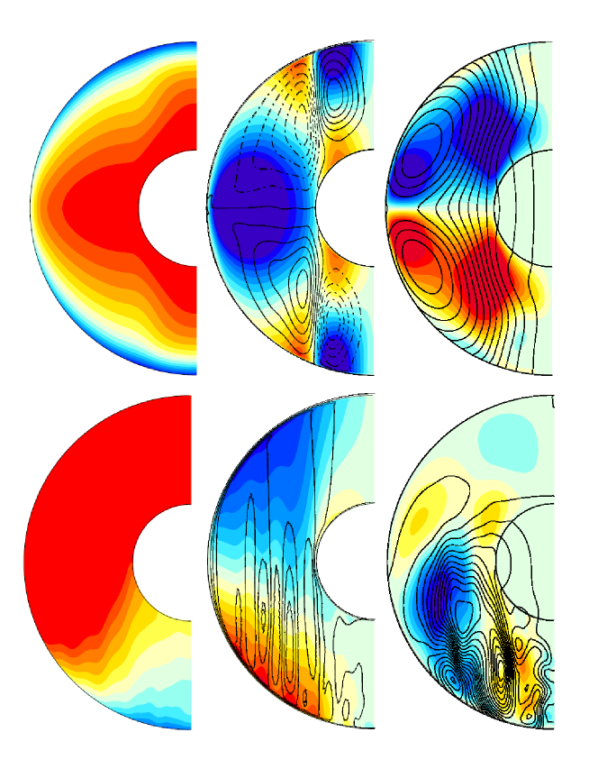
Figure 1: Zonal average of the temperature (left plots), zonal flow with meridional circulation contours (middle plots) and toroidal field with poloidal field line contours (right plots) for columnar convection dominated and magnetic dipolar reference case (left) and a typical hemispherical dynamo solution with the strong EAA symmetry in the flow (right). See the online-version of the article for the color figure.

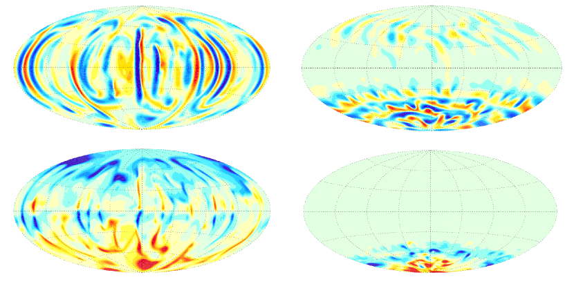
Figure 2: Radial flow (top row) at mid-depth and radial field at CMB (lower row) for the columnar reference case (left) and the hemispherical dynamo (right), indicates the reduction of the magnetic signature at the CMB if the radial motions are limited to the southern polar cusp of high heat flux. Here an Aitoff projection of the spherical CMB is used. See the online-version of the article for the color figure.

Figure 1 and 2 illustrate the typical hemispherical dynamo configuration emerging at $g=100\%$ and compares this with the typical dipole dominated dynamo found at $g=0\%$. While the southern hemisphere is still cooled efficiently the northern hemisphere remains hot since radial upwellings and the associated convective cooling are predominantly concentrated in the southern hemisphere (figure 2, top row). The flow pattern changes from classical columnar solutions to a thermal wind dominated flow which is a direct consequence of the strong north/south temperature gradient (figure 1, left bottom). When neglecting inertial, viscous and Lorentz force contributions the azimuthal component of the curl of the Navier-Stokes equation (1) yields:

$$2\frac{\partial\bar{u}_{\phi}}{\partial z}=\frac{RaE}{Pr}\frac{1}{r_{cmb}}\frac{\partial\bar{T}}{\partial\vartheta}\;\;.$$ (10)

This is the thermal wind equation and the respective zonal flows will dominate the solution, indicated by large $\mathcal{A}$ values when the latitudinal temperature gradient is large enough (Landeau and Aubert, 2011). Since radial flows mainly exist in the southern hemisphere the production of poloidal and thus radial magnetic field is also concentrated there. This results in a very hemispherical magnetic field pattern at the top of the dynamo region (figure 2, bottom row).

The figure 3 demonstrates that the toroidal energy rises quickly with the variation amplitude $g$ while the poloidal energy is much less effected. The growth of the toroidal energy is explained by the increasing thermal wind, which is an equatorial anti-symmetric and axisymmetric (EAA) toroidal flow contribution. At a disturbance amplitude of $g=60\%$ the EAA contribution accounts for already $50\%$ of the total kinetic energy (figure 3.b ). The maximum EAA contribution of $\mathcal{A}\approx 0.8$ is reached at $g=100\%$. When further increasing the variation amplitude, the thermal wind still gains in speed. However, the relative importance of the EAA mode decreases because the strongest latitudinal temperature gradient and thus the thermal wind structure moves further south. This trend is already observed in figure 1.

The equatorial anti-symmetry of the poloidal kinetic energy rises from $10\%$ for $g=0$ to about $50\%$ for $g=100$% reflecting that upwellings are increasingly concentrated in one (southern) hemisphere. The meridional circulation remains weak (figure 3.d), and its contribution to the total EAA energy is minor.

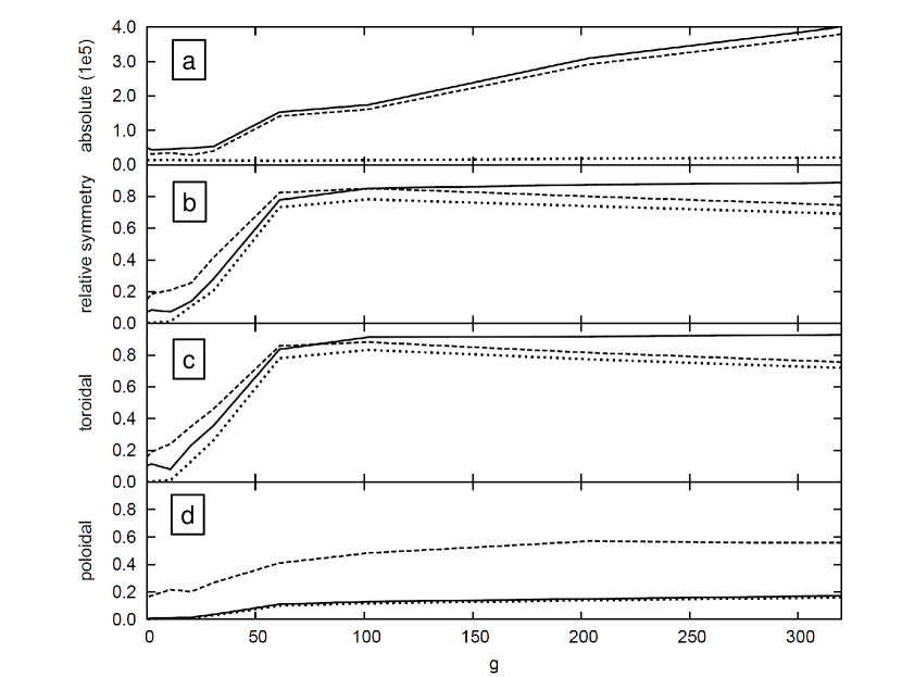
Figure 3: Symmetries and amplitude of total kinetic energy and toroidal/poloidal contributions as a function of $g$. a) total (solid line), toroidal (dashed) and poloidal (dotted) kinetic energy; b) relative amount of axisymmetry (solid), equatorial anti-symmetry (dashed) and the combined symmetries (EAA, dotted) of the full kinetic energy; c) and d) show the same but separated into toroidal and poloidal contributions.

3.2 Dynamo mechanism

The upper panel in figure 4 demonstrates that the rise in the magnetic Reynolds number $Rm$, that goes along with the increasing toroidal flow amplitude, does not necessarily lead to higher Elsasser numbers. Once more, cases at $E=10^{-4}$, $Ra=4.0\times 10^{7}$ and $Pm=2$ are depicted here. For small variation amplitudes up to $g=30$% $\Lambda$ still increases due to the additional $\Omega$-effect associated to the growing thermal winds. Figure 4 (lower panel) shows that the relative contribution of the $\Omega$-effect to toroidal field production $\mathcal{O}$ grows with $g$. For $g=0$ it is rather weak so that the dynamo can be classified as $\alpha^{2}$ (Olson et al., 1999). Around $g=50\%$, $\mathcal{O}$ reaches $50\%$ and the dynamo is thus of an $\alpha^{2}\Omega$-type. When increasing $g$ further the classical convective columns practically vanish and the associated $\alpha$-effects decrease significantly, leading to both weak poloidal and toroidal fields (figure 4, lower panel). For the toroidal field the effect is somewhat compensated by the growing $\Omega$-effect. The hemispherical dynamo clearly is an $\alpha\Omega$-dynamo.

At $g=100\%$ the hemispherical mode clearly dominates and the dynamo is of the $\alpha\Omega$-type with $\mathcal{O}\approx 0.8$. The Elsasser number has dropped to half its value at $g=0$ while the magnetic Reynolds number has increased by a factor two (figure 4, upper panel). The hemispherical dynamo is clearly less effective than the columnar dynamo.

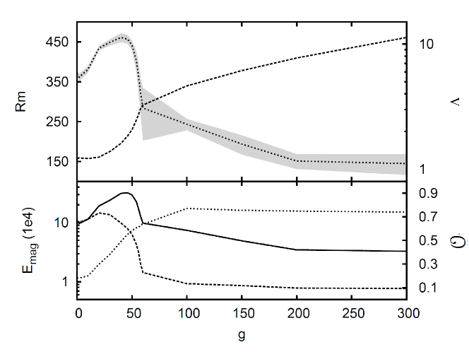
Figure 4: Upper panel: Flow amplitude in terms of the magnetic Reynolds number (solid line) and magnetic field strength in terms of Elsasser number (dashed)) as function of the CMB heat flux anomaly amplitude $g$, shows the difference between both dynamo regimes in the efficiency of inducing a dynamo. The hemispherical solution, with the $\alpha\Omega$-induction contains large amounts of axisymmetric zonal flows created by the Coriolis force, therefore the kinetic energy is drastically larger than in the columnar regime ($g=0$). The magnetic energy decreases, the more the $g$ increases. The gray shade correspond to the standard deviation due to time variability.
Lower panel: Toroidal (dashed) and poloidal (solid) magnetic field in nondimensional units and the relative $\Omega$-effect in terms of $\mathcal{O}$ (dotted) as a function of $g$ demonstrates the transformation of induction characteristic from an $\alpha^{2}$-dynamo at $g=0$ (columnar dynamo) towards an $\alpha\Omega$-type from $g=60\%$ (hemispherical solution).

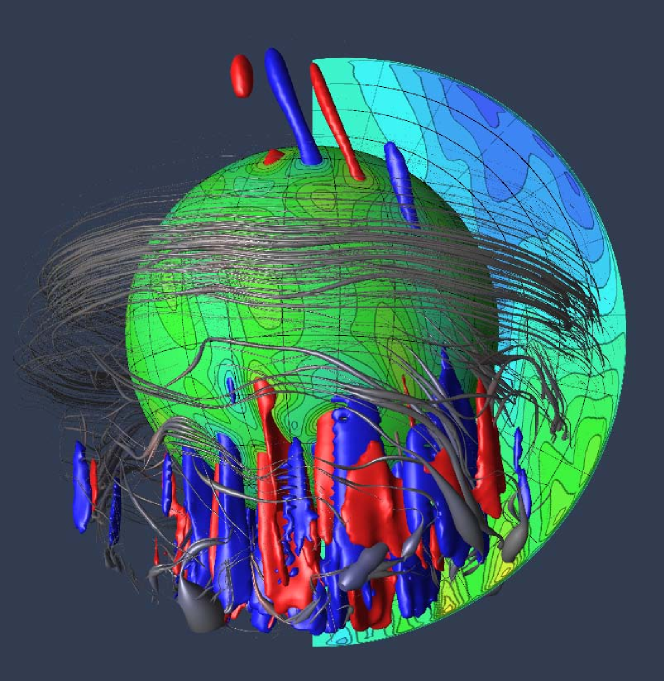
Figure 5: 3D visualization of flow and magnetic field generation in a hemispherical dynamo. The meridional cut depicts contours of axisymmetric zonal flows with prograde (retrograde) directions shown in yellow/red (blue). Outward (inward) radial flows are shown as yellow/red (blue) contours of a spherical shell at mid depth $r_{icb}+(r_{cmb}-r_{icb})/2$. Red (blue) isosurfaces depict the 3D structure of convective upwellings (downwellings). Gray fieldlines illustrate the magnetic field configuration. Their thickness is scaled with the local magnetic field energy. See the article online-version for the color figure.

Figure 5 illustrates the hemispherical dynamo mechanism in a 3D rendering. Magnetic field lines show the magnetic field configuration, their thickness is scaled with the local magnetic energy while red and blue colors intensities indicate the relative inward and outward radial field contribution. Plain gray lines are purely horizontal. Red and blue isosurfaces characterize inward and outward directed radial plume-like motions producing radial field magnetic field. Strong axisymmetric zonal field is produced by a thermal wind related $\Omega$-effect around the equatorial plane.

3.3 Magnetic Oscillations

Figure 6 illustrates the changes in the time behavior of the poloidal magnetic field when the CMB heat flux variation is increased. We concentrate on axisymmetric Gaussian coefficients at the CMB $(r=r_{cmb})$ here. In the reference case $g=0$ (top panel) the axial dipole dominates, varies chaotically in time and never reverses. If $g$ is increased to $50\%$ (second panel) the relative importance of the axial quadrupole component has increased significantly, which indicates the increasing hemisphericity of the magnetic field. To yield a hemispherical magnetic field a similar amplitude in dipolar (equatorial antisymmetric) and quadrupolar (equatorial symmetric) dynamo family contributions is required (Landeau and Aubert, 2011; Grote and Busse, 2000).

When increasing the variation slightly to $g=60\%$ (third panel) where the hemispherical mode finally dominates, all coefficients assume a comparable amplitude and oscillate in phase around a zero mean with a period of roughly half a magnetic diffusion time. The faster convective flow variations can still be discerned as a smaller amplitude superposition in figure 6.

The oscillation is also present in a kinematic simulation performed for comparison and is thus a purely magnetic phenomenon. Lorentz forces nevertheless cause the flow to vary along with the magnetic field. Since the coefficients vary in phase there are times where the magnetic field and thus the Lorentz forces are particularly weak or particularly strong. Figure 7 illustrates the solutions at maximum (top) and minimum (middle) rms field strength. At the minimum the convective columns are still clearly present and the flow is similar to that found in the non-magnetic simulations shown in the lower panel of figure 7. At the maximum the Lorentz forces, in particular those associated with the strong zonal toroidal field, severely suppress the columns. The magnetic field thereby further promotes the dominance of the hemispherical mode (Landeau and Aubert, 2011). This becomes even more apparent when comparing the relative importance of the EAA mode $\mathcal{A}$ in magnetic and non-magnetic simulations in the top panel of figure 8. In the dynamo run $\mathcal{A}$ is around $35\%$ higher than in the non-magnetic case for mild heat flux variation amplitudes.

When further increasing the amplitude of the CMB heat flux pattern, the frequency grows, the time behavior becomes somewhat more complex, and the different harmonics vary increasingly out of phase. In addition, the relative importance of harmonics higher than the dipole increase which indicates a concentration of the field at higher southern latitudes. The impact of the oscillations on the flows decreases since the hemispherical mode now always clearly dominates and the relative variation in the magnetic field amplitude becomes smaller.

The appearance of the oscillations may result from the increased importance of the $\Omega$-effect which at $g=60$% starts to dominate toroidal field production (see figure 4, lower panel). The $\Omega$-effect could be responsible for the oscillatory behavior of the solar dynamo as has, for example, been demonstrated by Parker (1955) who describes a simple purely magnetic wave phenomenon. Busse and Simitev (2006) report Parker wave type oscillatory behavior in their numerical dynamo simulations where the stress free mechanical boundary conditions promote strong zonal flows and thus a significant $\Omega$-effect.

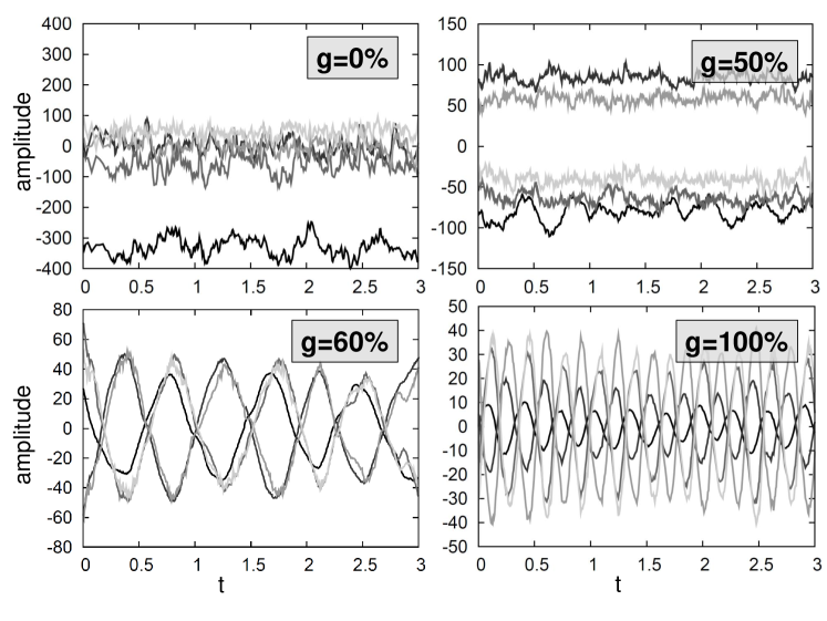
Figure 6: Time evolution of the first five axisymmetric Gauss coefficients at the CMB for the dipole dominated ($g=0$%,$50$%) (first and second panel), the oscillatory ($g=60$%, third panel) and the reversing hemispherical regime ($g=100$% bottom). The colours indicate different spherical harmonic degrees $l$: black $l=1$, dark gray $l=2$, gray $l=3$, light gray $l=4$, faint gray $l=5$.

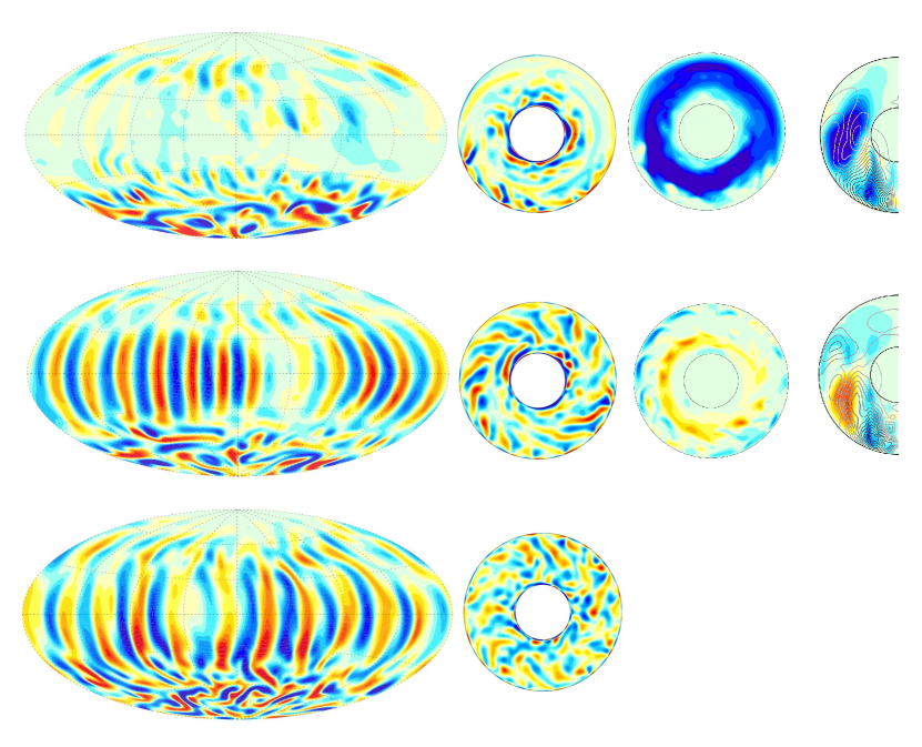
Figure 7: The upper two rows depict the solution at $g=60$% at maximum ($\Lambda=12$) and minimum magnetic field amplitude ($\Lambda=0.06$) respectively. The lower row shows a non-magnetic simulation at identical parameters for comparison. Each row shows from left to right: the radial flow at mid depth in the shell, the z-vorticity in the equatorial plane, the azimuthal magnetic field at the equator and the zonal toroidal field. See the online-version of the article for the color figure.

3.4 Arbitrary tilt angle

To explore to which degree the effects described above still hold when the variation and rotation axis do not coincide we systematically vary the variation pattern tilt angle $\alpha$ (see eq. 5) up to 90 degrees. The lower panel in figure 8 shows how $\mathcal{A}$, the relative EAA kinetic energy, varies with $g$ for different tilt angles. Somewhat surprisingly, the hemispherical mode still clearly dominates for tilt angles up to $\alpha=80^{\circ}$. Only the rather special case of $\alpha=90^{\circ}$ shows a new behavior, where $\mathcal{A}$ remains negligible. It is thus the general breaking of the north/south symmetry that is essential here. Since it leaves the northern hemisphere hotter than the southern it always leads to the above described dynamo mode.

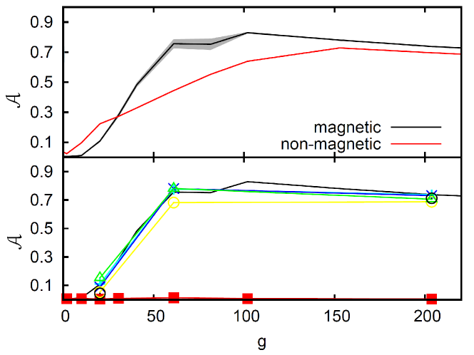
Figure 8: upper panel : Effect of the Lorentz force on the relative kinetic energy in the EAA mode for dynamo (black) and non-magnetic (gray) simulations. The time variability is indicated by gray shaded areas in the width of the standard deviation. The magnetic oscillation described in the text lead to the stronger time variability in the dynamo simulations at $g=60$% and $g=100$%.
lower panel: The relative equatorially anti-symmetric and axisymmetric energy for different tilting angles follows the onset of EAA convective mode in the case for the axial pattern (black line). For the equatorial orientation (squares) the EAA contribution to total kinetic energy remains Zero. Triangles - $10^{\circ}$, crosses - $30^{\circ}$, faint circles- $45^{\circ}$, dark circles - $60^{\circ}$, plus symbols - $80^{\circ}$. See the online-version of the article for the color figure.

The $90$ degree tilt angle of the $(l=1,m=1)$ pattern forms a special case because the breaking of the north-south symmetry is missing here. Finally, the effects of the east/west symmetry breaking become apparent and supersede the thermal wind related action in the other cases. Figures 9 and 10 illustrate the solution for an equatorial anomaly with $g=200\%$.

The resulting east/west temperature difference drives a large scale westward directed flow and a more confined eastward flow in the equatorial region of the outer part of the shell (figure 9). Coriolis forces divert the westward directed flow poleward and inward, and lead to the confinement of the eastward directed flow. Consequently, the westward flow plays the more important role here.

The diverted flows feed two distinct downwelling features that form at the latitude of zero heat flux disturbance close to the tangent cylinder. Due to the significant time dependence of the solution these can best be identified in time average flows shown in figure 10. Convective columns concentrated in the high heat flux hemisphere but the center of their action is somewhat shifted retrograde, probably due to the action of azimuthal winds. Other authors have shown that this shift, for example, depends on the Ekman number (Christensen and Olson, 2003). The remaining columns are small scale and highly time dependent. On time average only one column-like feature remains, identified by a strong downwelling somewhat west to the longitude of highest heat flux.

The time averaged flows form two main vorticity structures illustrated in figure 10. A long anticyclonic structure associated to the strong equatorial westward flow stretches nearly around the globe and connects the equator with high latitudes inside the tangent cylinder. A smaller cyclonic feature is owed to the eastward equatorial flow.

The snapshot and time averaged radial magnetic fields shown in figure 10 are rather similar which demonstrates that the time dependent small scale convective features are not very efficient in creating larger scale coherent magnetic field. The radial field is strongly concentrated in patches above flow downwelling where the associate inflows concentrate the background field (Olson et al., 1999). Like in the study for dynamos with homogeneous CMB heat flux by Aubert et al. (2008) the anti-cyclone mainly produces poloidal magnetic field. The cyclone twists the field in the other direction and therefore is responsible for the pair of inverse (outward directed here) field patches located at mid latitudes in the western hemisphere. The exceptional strength of the high latitude normal flux patches suggests that additional field line stretching further intensified the field here.

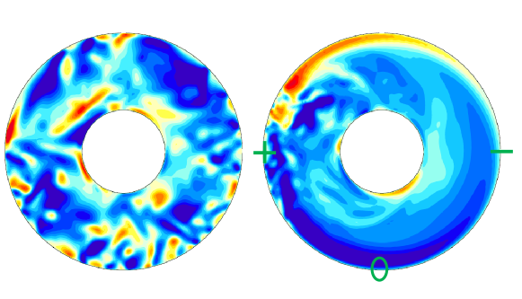
Figure 9: Equatorial slice of $u_{\phi}$ for the homogeneous reference case (left) and the equatorial heat flux anomaly (right). The plus, minus and zero character describe the maximal, minimal and the zero line of the anomaly. See the online-version of the article for the color figure.

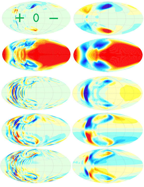
Figure 10: Aitoff projections of spherical surfaces of (from top to bottom) radial field, temperature (both at the CMB), $u_{r}$, $u_{\vartheta}$ and z-vorticity at $r/r_{cmb}=0.8$ for a snapshot (left plots) and the time average (right). Parameters: $Ra=4\times 10^{7}$, $E=10^{-4}$, $Pm=2$, equatorial ($l=m=1$) perturbation with $g=100\%$ relative amplitude. See the online-version of the article for the color figure.

3.5 Parameter Dependence

Focusing again at the axial heat flux anomaly we further study the influence of Rayleigh $Ra$, Ekman $E$ and magnetic Prandtl number $Pm$. In general we find that, independently of the Ekman $E$ and Rayleigh numbers $Ra$, a hemispherical dynamo mode is promoted once $g$ reaches a value of $60\%$. Close to the onset of dynamo action a mild variation can help to maintain dynamo action due to the additional $\Omega$-effect. See the cases at $E=10^{-4}$ and either $Ra=7\times 10^{6}$, $Pm=2$ or $Ra=2\times 10^{8}$, $Pm=1$ in table LABEL:Tab1. A strong amplitude of the heat flux anomaly can also suppress dynamo action due to the weakening of convective columns by the Lorentz force. For example, at $E=10^{-4}$, $Ra=4\times 10^{7}$ and $Pm=2$ the dynamo fails once $g$ reaches $200\%$.

Figure 11 shows how the CMB and surface hemisphericity ($\mathcal{H}_{cmb}$ , $\mathcal{H}_{sur}$ ) depends on the magnetic Reynolds number ${Rm^{\star}}$ based on the equatorially anti-symmetric part of the zonal flow only and therefore useful to quantify the important $\Omega$-effect in the hemispherical dynamo cases.

For $E=10^{-4}$ the $\mathcal{H}_{cmb}$ values first increase linearly with ${Rm^{\star}}$ and then saturates around $\mbox{$\mathcal{H}_{cmb}$}\approx 0.75$ for $\mbox{${Rm^{\star}}$}\geq 400$. All cases roughly follow the same curve with the exception of the peculiar $Ra=7\times 10^{6}$, $Pm=2$ and $g=60$% case described above. This means that there is a trade off between $g$, $Ra$ and $Pm$; increasing either parameter leads to larger ${Rm^{\star}}$ values. All the solution with hemisphericities $\mbox{$\mathcal{H}_{cmb}$}\ >0.6$ oscillate.

The few simulations at smaller Ekman numbers indicate that the degree of hemisphericity decreases with decreasing $E$. This is to be expected since the Taylor Proudman theorem becomes increasingly important (Landeau and Aubert, 2011), inhibiting the ageostrophic hemispherical mode. Larger heat flux variation amplitudes can help to counteract this effect. Since both inertia and Lorentz forces can help to balance the Coriolis force, increasing either $Ra$ or $Pm$ also helps. For $E=3\mbox{$\times 10^{-5}$}$ an oscillatory case with $\mbox{$\mathcal{H}_{cmb}$}=0.76$ is found for the larger Rayleigh number of $Ra=4\mbox{$\times 10^{8}$}$ and $g=100$%. For $E=10^{-5}$ $\mathcal{H}_{cmb}$ remains small at $g=100$% and we could not afford to increase $Ra$ here since larger $Ra$ as well as lower $E$ values both promote smaller convective and magnetic length scales and therefore require finer numerical grids.

The decrease in length scales has another interesting effect on the radial dependence of hemisphericity. To yield a maximum hemisphericity, equatorially symmetric ($l+m=$ even) and anti-symmetric ($l+m=$ odd) magnetic field contributions must be of comparable strength, i.e. obey a ’whitish’ spectrum (in a suitable normalization) (Grote and Busse, 2000). Since, however, the radial dependence of the modes depends on the spherical harmonic degree (they decay like $r^{-(l+2)}$ away from the CMB) the hemisphericity also depends on radius. The spectrum can only be perfectly ’white’ at one radius. The smaller the scale of the magnetic field at $r_{cmb}$ the further this radius lies beyond $r_{cmb}$. This explains why the $\mathcal{H}_{sur}$ values shown in the lower panel of figure 11 show a much larger scatter than the $\mathcal{H}_{cmb}$ values. Larger values of $Ra$, $E$, but also $g$ and $Pm$ lead to small magnetic scales and thus larger ratios of $\mathcal{H}_{sur}$ over $\mathcal{H}_{cmb}$.

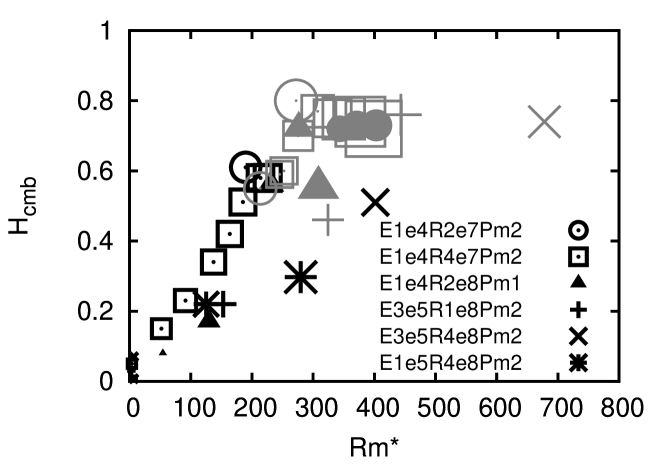
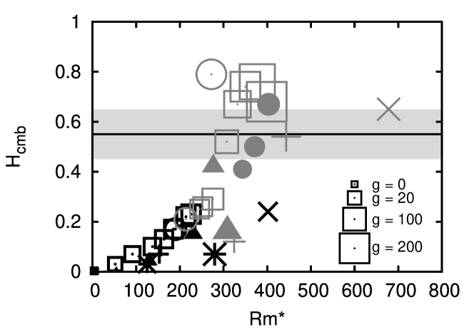
Figure 11: Top panel: Hemisphericity at CMB versus ${Rm^{\star}}$, the magnetic Reynolds number based on the equatorially anti-symmetric thermal wind. Oscillatory dynamos in gray, stationary in black symbols.
bottom panel: Hemisphericity at the (imaginary) Martian surface versus ${Rm^{\star}}$.

4 Application to Mars

Could the hemispherical dynamo models presented above provide an explanation for the crustal magnetization found on Mars? To address this question we rely on the hemisphericity of the crustal magnetization and the magnetic field strength inferred from Martian meteorites. Amit et al. (2011) use MGS data to estimate a hemisphericity between $\mbox{$\mathcal{H}_{sur}$}=0.45$ and $\mbox{$\mathcal{H}_{sur}$}=0.65$. The magnetization of the Martian meteorite (ALH 84001) suggest a field strength of the ancient dynamo between $5$ and $50\,\textrm{$\mu$T}$ (Weiss et al., 2002).

Because our simulations show that the magnetic field strength also varies significantly with the amplitude of the heat flux pattern, we rescale the dimensionless field strength in our simulations by assuming that the Elsasser number provides a realistic value. Assuming a magnetic diffusivity of $\lambda=1.32\,$m${}^{2}\,$s^-1 and density of $\rho=7000\,$kg m^-3, a rotation rate of $\Omega=7.1\times 10^{-5}\,$s^-1 and the magnetic vacuum permeability then allows to rescale the Elsasser number to dimensional field strengths. Time is rescaled via the magnetic diffusion time $t_{\lambda}=D^{2}\lambda^{-1}$ with an outer core radius of $1680\,$km.

We have included the Martian crustal hemisphericity values in the lower panel of figure 11 to show that only oscillatory cases fall in the required range with heat flux variation amplitudes $g\geq 60$% and $\mbox{${Rm^{\star}}$}\geq 300$. Figure 12 shows the temporal evolution of $\mathcal{H}_{cmb}$ and $\mathcal{H}_{sur}$ for one of these cases. The variation is surprisingly strong and oscillates at twice the frequency of the individual Gauss coefficients. Since all coefficients roughly oscillate with the same period there are two instances during each period where the hemisphericity is particularly large (around $\mbox{$\mathcal{H}$}\approx 0.8$) since axial dipole and quadrupole have the same amplitude. Since the mean hemisphericity decreases with radius the variation amplitude is much higher at the planetary surface than at the CMB (figure 12). The strong time dependence of oscillatory cases highlights that considerations over which period the magnetization was acquired are extremely important.

Figure 12: Time evolution of hemisphericity $\mathcal{H}$ at the CMB (solid) and surface (dashed) for $g=100\%$, $Ra=4\times 10^{7}$, $E=10^{-4}$ and $Pm=2$.

To translate the dynamo field into a magnetization pattern, Amit et al. (2011) suggest two end-members of how the magnetization was acquired. In the first end-member scenario called ’random’ the crustal magnetization is acquired randomly in time and space and, according to Amit et al. (2011), should reflect the time averaged intensity. In the second end-member called ’continuous’, magnetization is acquired in global thick layers, so that the time intensity of the time average field is considered. However, since the magnetization records the magnetic changes happening during the slow crust formation, the local net magnetization, as seen by an observer, is always proportional to the time averaged local magnetic field possibly slightly dominated by the outermost layers. We therefore think, that the random magnetization scenario does not apply. The strong magnetization found on Mars indicates that a significant portion of the crust is unidirectionally magnetized. Langlais et al. (2004) estimated a magnetization depth of $20-40\,$km depending on the magnetization density. Crust formation is a rather slow process that may take millions of years. Typical magnetic time scales can be much shorter. The periods of the reversing strongly hemispherical dynamos discussed above, amount to not more than about ten thousand years.

Table LABEL:Tab1 lists the time averaged rescaled magnetic field intensity at the model Martian surface. For $g\leq 60$% the field strengths are similar to that predicted for Mars (Weiss et al., 2002) and fall somewhat below this values for larger $g$-values. In the strongly hemispherical oscillating cases, however, the amplitude of the time average field average to zero on time scales of the crustal magnetization. We therefore conclude that while the hemispherical dynamos can reach hemisphericities similar to that of the Martian crustal magnetization their oscillatory nature makes them incompatible with the rather strong magnetization amplitude.

5 Discussion

We find that an equatorially anti-symmetric convective mode is consistently triggered by a cosine heat flux variation that allows more heat to escape through the southern than through the northern outer boundary of the dynamo region. When the variation is strong enough, convective up- and down-wellings are concentrated at the southern hemisphere and the northern hemisphere remains hot. The associated latitudinal temperature gradients drive strong thermal winds that dominate the flow when, for example, the variation amplitude $g$ exceeds $50\,$% at $E=10^{4}$. Tilting the heat flux pattern axis leaves the solution more or less unchanged with the exception of the $90^{\circ}$-case where the equatorial symmetry remain unbroken. We conclude that breaking the equatorial symmetry is dynamically preferred over an equatorially oriented heat flux anomaly of the CMB heat flux.

Due to the thermal winds, the dynamo type changes from $\alpha^{2}$ to $\alpha\Omega$ but is generally less efficient. Lorentz forces associated with the toroidal field created via the $\Omega$-effect tend to kill whatever remains of classical columnar convection. This further increases the equatorial anti-symmetry of the solution. Poloidal fields are mainly produced by the southern up- and downwellings which lead to a hemispherical field pattern at the outer boundary.

When the hemisphericity approaches values of that found in Martian crustal magnetization, however, all dynamos start to oscillate on (extrapolated) time scales of the order of $10\,$kyr. These oscillations are reminiscent of previously described Parker waves in dynamo simulations (Busse and Simitev, 2006). As a typical characteristic of Parker waves, the frequency increases with the (square root of the) shear strength, see table LABEL:Tab1. The oscillation periods are much shorter than the time over which the deep reaching Martian magnetization must have been acquired (Langlais et al., 2004). Being a composite of many consecutive layers with alternating polarities the net magnetization would scale with the time averaged field and would therefore likely be much smaller than the predicted strength of the ancient Martian field magnetizing the crust (Weiss et al., 2002). The maximum hemisphericity for non-oscillatory dynamos amounts to a configuration where the mean northern field amplitude is only $50\%$ weaker than the southern. Additional effects like lava-overflows would then be required to explain the observed hemisphericity.

Amit et al. (2011); Stanley et al. (2008) also studied the effects of the identical sinusoidal boundary heat flux pattern and find very similar hemispherical solutions. Amit et al. (2011) used a very similar setup to ours and also reported oscillations when the dynamo becomes strongly hemispherical. Stanley et al. (2008) do not report the problematic oscillations intensively studied here, which may have to do with differences in the dynamo models. They study stress-free rather than rigid flow boundaries and assume that the growing inner core contributes to drive the dynamo while our model exclusively relies on internal heating. Should a hemispherical dynamo indeed be required to explain the observed magnetization dichotomy, this may indicate that ancient Mars already had an inner core. Alternatively efficient demagnetization mechanisms may have modified an originally more or less homogeneous magnetized crust (Shahnas and Arkani-Hamed, 2007).

Landeau and Aubert (2011) observed that similar hemispherical dynamos are found when the Rayleigh number exceeds a critical value. However, albeit the effects are significantly smaller than when triggered via the boundary heat flux. All the cases explored here remain below this critical Rayleigh number. Landeau and Aubert (2011) also mentioned that the equatorial anti-symmetry, and thus the hemisphericity of the magnetic field, decreases when the Ekman number is decreased. Our simulations at lower Ekman number seem to confirm this trend although a meaningful extrapolation to the Martian value of $E=3\times 10^{-15}$ would require further simulations at lower Ekman numbers. To a certain extent the decrease can be compensated by increasing the heat flux variation amplitude, the Rayleigh number or the magnetic Prandtl number.

Our results show that a north-south symmetry breaking induced by lateral CMB heat flux variations can yield surprisingly strong effects. Fierce thermal winds and local southern upwellings take over from classical columnar convection and the dynamo changes from an $\alpha^{2}$ to an $\alpha\Omega$-type. The dominant $\Omega$-effect seems always linked to Parker-wave-like field oscillations typically discussed for stellar applications. It will be interesting to further explore the aspects independent of the application to Mars.

References

- Acuña et al. [1999] M. H. Acuña, J. E. P. Connerney, N. F. Ness, R. P. Lin, D. Mitchell, C. W. Carlson, J. McFadden, K. A. Anderson, H. Reme, C. Mazelle, D. Vignes, P. Wasilewski, and P. Cloutier. Global Distribution of Crustal Magnetization Discovered by the Mars Global Surveyor MAG/ER Experiment. Science, 284:790–793, April 1999. 10.1126/science.284.5415.790.
- Acuña et al. [2001] M. H. Acuña, J. E. P. Connerney, P. Wasilewski, R. P. Lin, D. Mitchell, K. A. Anderson, C. W. Carlson, J. McFadden, H. Rème, C. Mazelle, D. Vignes, S. J. Bauer, P. Cloutier, and N. F. Ness. Magnetic field of Mars: Summary of results from the aerobraking and mapping orbits. Journal of Geophysical Research, 106:23403–23418, October 2001. 10.1029/2000JE001404.
- Amit and Olson [2006] H. Amit and P. Olson. Time-average and time-dependent parts of core flow. Physics of the Earth and Planetary Interiors, 155:120–139, April 2006. 10.1016/j.pepi.2005.10.006.
- Amit et al. [2011] H. Amit, U. R. Christensen, and B. Langlais. The influence of degree-1 mantle heterogeneity on the past dynamo of Mars. Physics of the Earth and Planetary Interiors, 189:63–79, November 2011. 10.1016/j.pepi.2011.07.008.
- Arkani-Hamed and Olson [2010] J. Arkani-Hamed and P. Olson. Giant impact stratification of the Martian core. Geophysical Research Letters, 37:2201–2205, January 2010. 10.1029/2009GL041417.
- Aubert et al. [2008] J. Aubert, J. Aurnou, and J. Wicht. The magnetic structure of convection-driven numerical dynamos. Geophysical Journal International, 172:945–956, March 2008. 10.1111/j.1365-246X.2007.03693.x.
- Aubert et al. [2009] J. Aubert, S. Labrosse, and C. Poitou. Modelling the palaeo-evolution of the geodynamo. Geophysical Journal International, 179:1414–1428, December 2009. 10.1111/j.1365-246X.2009.04361.x.
- Bloxham [2000] J. Bloxham. Sensitivity of the geomagnetic axial dipole to thermal core-mantle interactions. Nature, 405:63–65, May 2000.
- Braginsky and Roberts [1995] S. I. Braginsky and P. H. Roberts. Equations governing convection in earth’s core and the geodynamo. Geophysical and Astrophysical Fluid Dynamics, 79:1–97, 1995. 10.1080/03091929508228992.
- Breuer et al. [2010] D. Breuer, S. Labrosse, and T. Spohn. Thermal Evolution and Magnetic Field Generation in Terrestrial Planets and Satellites. Space Sci. Rev., 152:449–500, May 2010. 10.1007/s11214-009-9587-5.
- Busse and Simitev [2006] F. H. Busse and R. D. Simitev. Parameter dependences of convection-driven dynamos in rotating spherical fluid shells. Geophysical and Astrophysical Fluid Dynamics, 100:341–361, October 2006. 10.1080/03091920600784873.
- Christensen and Olson [2003] U. R. Christensen and P. Olson. Secular variation in numerical geodynamo models with lateral variations of boundary heat flow. Physics of the Earth and Planetary Interiors, 138:39–54, June 2003. 10.1016/S0031-9201(03)00064-5.
- Christensen et al. [2007] U. R. Christensen, J. Aubert, and P. Olson. Convection-driven planetary dynamos. In T. Kuroda, H. Sugama, R. Kanno, & M. Okamoto, editor, IAU Symposium, volume 239 of IAU Symposium, pages 188–195, May 2007. 10.1017/S1743921307000403.
- Connerney et al. [2001] J. E. P. Connerney, M. H. Acuña, P. J. Wasilewski, G. Kletetschka, N. F. Ness, H. Rème, R. P. Lin, and D. L. Mitchell. The Global Magnetic Field of Mars and Implications for Crustal Evolution. Geophsyical Research Letters, 28:4015–4018, November 2001. 10.1029/2001GL013619.
- Dreibus and Wänke [1985] G. Dreibus and H. Wänke. Mars, a volatile-rich planet. Meteoritics, 20:367–381, June 1985.
- Glatzmaier et al. [1999] G. A. Glatzmaier, R. S. Coe, L. Hongre, and P. H. Roberts. The role of the Earth’s mantle in controlling the frequency of geomagnetic reversals. Nature, 401:885–890, October 1999. 10.1038/44776.
- Grote and Busse [2000] E. Grote and F. H. Busse. Hemispherical dynamos generated by convection in rotating spherical shells. Phys. Rev. E, 62:4457–4460, September 2000. 10.1103/PhysRevE.62.4457.
- Harder and Christensen [1996] H. Harder and U. R. Christensen. A one-plume model of martian mantle convection. Nature, 380:507–509, April 1996. 10.1038/380507a0.
- Hori et al. [2010] K. Hori, J. Wicht, and U. R. Christensen. The effect of thermal boundary conditions on dynamos driven by internal heating. Physics of the Earth and Planetary Interiors, 182:85–97, September 2010. 10.1016/j.pepi.2010.06.011.
- Keller and Tackley [2009] T. Keller and P. J. Tackley. Towards self-consistent modeling of the martian dichotomy: The influence of one-ridge convection on crustal thickness distribution. Icarus, 202:429–443, August 2009. 10.1016/j.icarus.2009.03.029.
- Kutzner and Christensen [2000] C. Kutzner and U. Christensen. Effects of driving mechanisms in geodynamo models. Geophysical Research Letters, 27:29–32, 2000. 10.1029/1999GL010937.
- Kutzner and Christensen [2004] C. Kutzner and U. R. Christensen. Simulated geomagnetic reversals and preferred virtual geomagnetic pole paths. Geophysical Journal International, 157:1105–1118, June 2004. 10.1111/j.1365-246X.2004.02309.x.