Connecting the Sun and the Solar Wind: The Self-consistent Transition of Heating Mechanisms

Abstract

We have performed a 2.5 dimensional magnetohydrodynamic simulation that resolves the propagation and dissipation of Alfvén waves in the solar atmosphere. Alfvénic fluctuations are introduced on the bottom boundary of the extremely large simulation box that ranges from the photosphere to far above the solar wind acceleration region. Our model is ab initio in the sense that no corona and no wind are assumed initially. The numerical experiment reveals the quasi-steady solution that has the transition from the cool to the hot atmosphere and the emergence of the high speed wind. The global structure of the resulting hot wind solution fairly well agree with the coronal and the solar wind structure inferred from observations. The purpose of this study is to complement the previous paper by Matsumoto & Suzuki (2012) and describe the more detailed results and the analysis method. These results include the dynamics of the transition region and the more precisely measured heating rate in the atmosphere. Particularly, the spatial distribution of the heating rate helps us to interpret the actual heating mechanisms in the numerical simulation. Our estimation method of heating rate turned out to be a good measure for dissipation of Alfvén waves and low beta fast waves.

1 Introduction

For years, extensive studies have been carried out on the coronal heating problem. The hot corona lies above the cool photosphere (Edlén, 1943), which can not be explained by thermal processes. Instead the mechanical energy injection from the surface convection motion is expected to maintain the hot corona by means of magnetic field. The coupling between the convection and the magnetic field transports free magnetic energy that will be converted to thermal energy in the upper atmosphere. To resolve the coronal heating problem, we should specify the physics that are responsible for releasing the free magnetic energy.

In this paper, we will focus on the atmosphere above the solar pole where the fast solar wind emanates. The magnetic field lines above the solar pole open up to the interplanetary space. One of the most plausible carriers of the magnetic free energy in the open field region is Alfvén waves, which was first proposed by Alfvén (1947). Recent observations have been accumulating several pieces of evidence of the existence of the propagating Alfvén waves in the solar atmosphere (Okamoto & De Pontieu, 2011). Propagation and dissipation of Alfvén waves in the solar atmosphere is quite complicated since the gravity and the magnetic field make highly inhomogeneous atmospheres. For 1 dimensional configuration, nonlinear steepening of Alfvén waves and the subsequent shock formation play an important role in wave dissipation (Hollweg et al., 1982; Kudoh & Shibata, 1999; Matsumoto & Shibata, 2010). Plenty of wave modes will emerge when we consider two dimensional configuration (Shibata, 1983; Rosenthal et al., 2002; Bogdan et al., 2003).

All the above numerical simulations adopt simplified energy equation. In the coronal loop, mechanical heating is balanced by the radiative cooling and thermal conduction. Enthalpy flux due to the existence of the solar wind is also important when we consider the open field structure (Hollweg, 1986). Therefore in order to obtain the atmospheric structure above the solar pole, we should treat the corona and the solar wind in a self-consistent way. One of the most important aspects of the self-consistent models is that these models can determine the mass loss rate from the sun given the boundary condition at the surface. If we can construct the appropriate mass loss model from the sun, the model could be very useful even for the stellar or the planetary atmospheres.

Pioneering works by Hammer (1982a, b) treated the corona and the solar wind simultaneously in a self-consistent way. Instead of using the artificial heating function, Hollweg (1986); Cranmer et al. (2007) adopted the physically based heating model from phenomenological turbulent theories. Heating models based on acoustic shocks (Suzuki, 2002) and MHD shocks (Suzuki, 2004) are also investigated. Time steady condition is relaxed to demonstrate the self-consistent reproduction of the hot coronal wind with fully dynamical 1D (Suzuki & Inutsuka, 2005, 2006) and 2D (Matsumoto & Suzuki, 2012) (hereafter referred to as MS12) MHD simulations.

MS12 suggested that the shock heating is dominant heating mechanisms in the chromosphere and the coronal bottom while the turbulent heating is important in the solar wind acceleration region. However, there are two problems in the way how MS12 estimate the heating rate in their simulation. First, MS12 used dimensional analysis based on turbulent theory when they estimate the incompressible heating rate. This method can include large uncertainty, which allows MS12 only to estimate the order of magnitude of the heating rate. Second, the dimensional analysis does not have ability to estimate the temporal and spatial variability of the heating rate. In order to overcome the problems in MS12, we have developed an alternative method to estimate the heating rate. The purpose of the present paper is to describe more detailed features on heating mechanisms by using the new estimation method. Moreover, we will describe detailed dynamic features which are not shown in MS12.

We begin in section 2 by describing our numerical models and corresponding assumptions. The time-averaged quasi-steady solution is shown in section 3 while the dynamic features relating to the coupling between waves and the transition region shall be discussed in section 4. Then the basic idea to derive the heating rate as a function of space and time is given in section 5, although the detailed method for discretization and test simulations are explained in appendix B. In section 6, we shall show the total amount and the spatial distribution of heating rate and discuss the possible mechanisms that actually happened in the numerical simulation. We continue in section 7 by discussing the validity of the heating mechanisms found in our numerical simulation, while in section 8 we summarize.

2 Model & Assumptions

All the numerical methods to integrate the basic equations in this paper are the same as that used in MS12. We will describe the method in more detailed way here. Throughout the paper, we will assume single fluid MHD to describe a flux tube extended from the photosphere to the interplanetary space. Although the photosphere and the chromosphere are partially ionized, the use of single fluid approximation can be justified by frequent collisions between protons and neutrals (e.g., Pandey & Wardle, 2008). Above the upper corona ($r-r_{\rm s}>r_{\rm s}$ or 7.0$\times$10² Mm), proton and electron will decouple due to weak collisionality. Even in that case, we continue to use single fluid MHD equations for simplicity. Since we do not include any explicit dissipation terms in our equations, all the dissipations come from shocks and discretization errors. The method to estimate the heating rate shall be discussed in section 5. In addition to ideal MHD formulation, we include the gravity from the Sun. The solar gravity produces a highly stratified atmosphere , which inevitably leads initially linear waves to nonlinear waves. We consider a flux tube at $\theta=\pi/2$ in the spherical coordinate. We rotate the axis of the spherical coordinate so that the pole of the spherical coordinate lies on the equator of the sun. This helps us to avoid the numerical difficulty in the polar region of the spherical coordinate when we treat polar region of the sun. We neglect rotation of the sun as well as macro-scale magnetic field in this study. We impose the translational symmetry in the $\theta$ direction ($\partial_{\theta}=0$) so that all the variables depend on radius ($r$), azimuthal angle ($\phi$), and time ($t$). Perturbations in $\theta$ direction is purely incompressible, namely Alfvén mode, and perturbations of $r$ & $\phi$ components consist of fast and slow MHD modes (see section 4). Then our basic equations can be described as follows.

$${\partial{\cal U}\over\partial t}+{\partial{\cal F}\over\partial r}+{\partial{\cal G}\over\partial\phi}={\cal S},$$ (1)

$${\cal U}=\left(\begin{array}[]{c}r^{2}\rho\\ r^{2}\rho V_{r}\\ r^{2}\rho V_{\theta}\\ r^{2}\rho V_{\phi}\\ r^{2}B_{r}\\ rB_{\theta}\\ rB_{\phi}\\ r^{2}E\end{array}\right)\equiv\left(\begin{array}[]{c}{\cal R}\\ {\cal M}_{r}\\ {\cal M}_{\theta}\\ {\cal M}_{\phi}\\ {\cal B}_{r}\\ {\cal B}_{\theta}\\ {\cal B}_{\phi}\\ {\cal E}\end{array}\right),$$ (18)

$${\cal S}=\left(\begin{array}[]{c}0\\ \left[-B_{\perp}^{2}+\rho V_{\perp}^{2}+2P_{\rm T}-{\rho GM/r}\right]\times r\\ \left(B_{r}B_{\theta}-\rho V_{r}V_{\theta}\right)\times r\\ \left(B_{r}B_{\phi}-\rho V_{r}V_{\phi}\right)\times r\\ 0\\ 0\\ 0\\ -\rho V_{r}GM+Q_{\rm cnd}+Q_{\rm rad}\end{array}\right),$$ (27)

$${\cal F}=\left(\begin{array}[]{c}\rho V_{r}\times r^{2}\\ \left(\rho V_{r}^{2}+P_{\rm T}-B_{r}^{2}\right)\times r^{2}\\ \left(\rho V_{\theta}V_{r}-B_{\theta}B_{r}\right)\times r^{2}\\ \left(\rho V_{\phi}V_{r}-B_{\phi}B_{r}\right)\times r^{2}\\ 0\\ \left(V_{r}B_{\theta}-V_{\theta}B_{r}\right)\times r\\ \left(V_{r}B_{\phi}-V_{\phi}B_{r}\right)\times r\\ \left[\left(E+P_{\rm T}\right)V_{r}-\left(\mn@boldsymbol{V}\cdot\mn@boldsymbol{B}\right)B_{r}\right]\times r^{2}\end{array}\right),$$ (36)

$${\cal G}=\left(\begin{array}[]{c}\rho V_{\phi}\times r\\ \left(\rho V_{r}V_{\phi}-B_{r}B_{\phi}\right)\times r\\ \left(\rho V_{\theta}V_{\phi}-B_{\theta}B_{\phi}\right)\times r\\ \left(\rho V_{\phi}^{2}+P_{\rm T}-B_{\phi}^{2}\right)\times r\\ \left(V_{\phi}B_{r}-V_{r}B_{\phi}\right)\times r\\ V_{\phi}B_{\theta}-V_{\theta}B_{\phi}\\ 0\\ \left[\left(E+P_{\rm T}\right)V_{\phi}-\left(\mn@boldsymbol{V}\cdot\mn@boldsymbol{B}\right)B_{\phi}\right]\times r\end{array}\right),$$ (45)

$$P_{\rm g} = {\rho k_{\rm B}T\over\mu m_{\rm H}},$$ (46)

$$E = {1\over 2}\rho V^{2}+{P_{\rm g}\over(\gamma-1)}+{B^{2}\over 2},$$ (47)

$$P_{\rm T} = P_{\rm g}+{B^{2}\over 2},$$ (48)

$$V_{\perp}^{2} = V_{\theta}^{2}+V_{\phi}^{2},$$ (49)

$$B_{\perp}^{2} = B_{\theta}^{2}+B_{\phi}^{2},$$ (50)

where all the symbols have standard meanings except for magnetic field, $B$, which is normalized by $\sqrt{4\pi}$. We adopt the specific heat ratio $\gamma$ of $5/3$ for mono-atomic molecules. At around 6,000 K or less, almost all of hydrogens are neutrals while they are completely ionized at the temperature above 10⁴ K. To mimic the real equation of states there, we define the mean molecular weight as a function of temperature to linearly connect fully ionized and neutral gases,

$$\mu=\left\{\begin{array}[]{c}1~{}~{}\left(T<6,000~{}{\rm K}\right)\\ \\ \left[3.5\left(1-4285.7/T\right)\right]^{-1}\\ \left(6,000~{}{\rm K}<T<10^{4}~{}{\rm K}\right)\\ \\ 0.5~{}~{}\left({\rm otherwise}\right)\end{array}\right..$$ (57)

As for the thermal conduction, we use the classical formulation for collisional plasma,

$$Q_{\rm cnd}=\nabla\cdot\left(\kappa_{0}T^{5/2}{\nabla T\cdot\mn@boldsymbol{B}\over B^{2}}\mn@boldsymbol{B}\right).$$ (58)

We choose $\kappa_{0}=10^{-6}$ in cgs unit, reasonable value of electrons for fully ionized plasma in thermal equilibrium (Braginskii, 1965). Heat transport across magnetic field lines is inhibited in equation (58). In the present study, we use this classical limit throughout all space, although the deviation from the the classical heat conduction could affect the temperature structure in the outer corona ($>10$ $r_{\rm s}$ or 7.0 $\times$ 10³ Mm) (see Hollweg, 1978). We also introduce radiative cooling as follows.

$$Q_{\rm rad}=\left\{\begin{array}[]{lc}-n^{2}\Lambda\left(T\right)&~{}(T>T_{\rm c}~{}\&~{}\rho<\rho_{\rm c})\\ -nn_{\rm c}\Lambda\left(T_{\rm c}\right)&({\rm otherwise})\end{array}\right.,$$ (61)

$$\begin{array}[]{cllc}\log_{10}\Lambda\left(T\right)&=-&127.3&\\ &+&56.57&\log_{10}T\\ &-&9.84&(\log_{10}T)^{2}\\ &+&0.5548&(\log_{10}T)^{3},\end{array}$$ (66)

where $n=\rho/m_{\rm H}$, $T_{\rm c}=4\times 10^{4}$ K, and $\rho_{\rm c}=4.9\times 10^{-17}$ g cm^-3. The term in the first line in equation (61) represents the radiative cooling for optically thin plasma of the coronal abundance (e.g., Landini & Monsignori Fossi, 1990) fitted by polynomials. The radiative loss function is shown in figure 1. The term in the second line of equation (61) is in proportion to $n$ and mimics the radiative cooling for optically thick plasma that was empirically derived by Anderson & Athay (1989). Basically, the treatment of the thermal conduction and the radiative cooling in our study is the same one as that used in Moriyasu et al. (2004); Suzuki & Inutsuka (2005, 2006); Antolin et al. (2008); Antolin & Shibata (2010).

Figure 1: The radiative loss function as a function of temperature.

We set up our initial atmosphere by solving the equations of hydrostatic equilibrium without magnetic field. The initial atmospheres have 10⁴ K all over the numerical domain, starting from the initial photospheric density of 10^-7 g cm^-3 at $r=r_{\rm s}$. Above the height of 11 Mm ($\sim$ 1.6 $\times 10^{-2}~{}r_{\rm s}$), the density profiles are forced to be proportional to $r^{-2}$. This is simply because the exponential density drop causes numerical difficulties in the higher atmosphere. At the photospheric surface, we impose the locally concentrated magnetic field that would correspond to the kilo Gauss patch at the photosphere. The exact profile along $\phi$ direction at the photosphere are shown with the solid line in Figure 2d. This initial profile is produced by the superposition of narrow positive Gaussian and wide negative Gaussian. The presence of the kilo Gauss patches is clearly confirmed by HINODE/SOT even in the polar coronal hole where the high speed solar wind originates from (Tsuneta et al., 2008; Shiota et al., 2012). The magnetic field above the photosphere is extrapolated by using potential field approximation (Figure 2b). The super-radial expansion of the flux tube reduces the field strength from $\sim$ 3$\times$10³ to 3 Gauss in the region below 4 Mm (Figure 2cd). Above $\approx$ 4 Mm (6$\times$10^-3 $r_{\rm s}$), the field strength decreases in proportion to $r^{-2}$. Since all the open field lines start from a single cell in the current resolution, we have performed test simulations to check the resolution dependence in appendix A. We found that as far as the energy flux at the corona is concerned, the results would not change drastically. The field strength 3 Gauss well below the TR could be weak compared with the usual polar field strength of $\sim$ 10 Gauss. This is just a computational issue. Since we solve thermal conduction implicitly, the time step is usually determined by the Alfvén crossing time of the radial grid around the transition region ($\sim 0.1$ sec in the current resolution). If we reduce the field strength, we can use a longer time step restricted by the CFL condition. Larger field strength will produce larger Poynting flux above, which can be potential source to heat the corona.

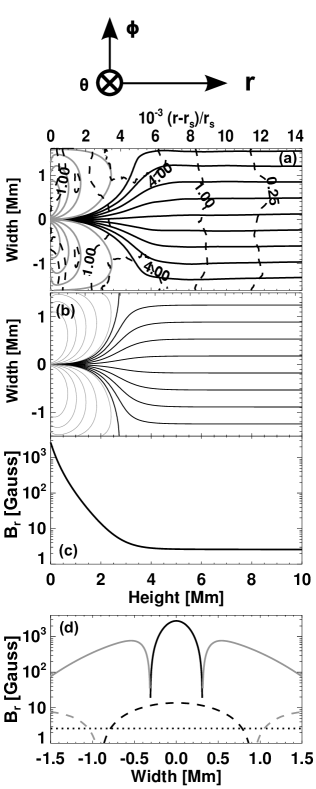
Figure 2: Magnetic field structure in our numerical simulation. (a) Mean magnetic field structure in the quasi-steady state below 10 Mm (1.4$\times$10^-2 $r_{\rm s}$). The black(gray) solid lines show open(closed) magnetic field lines. The black dashed lines indicate iso contours of plasma beta.The magnetic field lines (b) The initial magnetic field lines below 10 Mm (1.4$\times$10^-2 $r_{\rm s}$). The black(gray) solid lines represent the open(closed) field lines. (c) The radial magnetic field strength along $\phi=0$ as a function of height. (d) The radial magnetic field strength along the azimuthal direction. The solid, dashed, and dotted lines represent the field strength at $r-r_{\rm s}=0,2,6$ Mm (0, 2.9$\times$10^-3, 8.6$\times$10^-3 $r_{\rm s}$), respectively. The black/gray color means positive/negative value.

The horizontal length of our numerical domain is 3,000 km at the photosphere and it expands in proportion to $r$. 32 grid points are allocated to resolve 3,000 km so that the horizontal spatial resolution is nearly 100 km at the photosphere. Periodic boundary conditions are posed on the horizontal boundaries. As for the radial direction, we start our simulations from the photosphere ($r=r_{\rm s}$ or 7$\times$10² Mm) to the interplanetary space ($r=1,674~{}r_{\rm s}$ $>7$AU or 10⁶ Mm). The radial spatial resolution is 25 km at the photosphere. We increase the grid size non-uniformly ( 0.7 $r_{\rm s}$ or 490 Mm at 7 AU) as we go up higher to cover the whole numerical domain by using 16,384 grid points. The total number of the radial grid points are doubled from the previous simulation by MS12 to better resolve the wave propagation in the low corona. Open boundary in radial direction could be implemented by using characteristic method, although it is not straightforward to use characteristic method with thermal conduction. Instead, we take lengthy radial domain to avoid the numerical reflection from the top boundary and pose zero-derivative boundary condition there. At the final time of our simulation, the thermal conduction front reaches 4 AU (8.6$\times$10² r_s or 6$\times$10⁵ Mm) while the solar wind reaches 1 AU (2.2$\times$10² r_s or 1.5$\times$10⁵ Mm). Therefore, any physical information propagating from the inner boundary can not reach the top boundary within the duration we considered. In this paper we focus on the wind structure in $r<20$ $r_{\rm s}$ ($\sim 0.1$ AU, 1.4$\times$10⁴ Mm), which is in the quasi-steady state after sufficient Alfvén crossing time.

At the inner boundary, all the variables are fixed to the initial value except for the velocity in $\theta$ direction ($V_{\theta}$). The spectra of $V_{\theta}$ at the bottom boundary are prescribed to excite Alfvén waves. Throughout this paper, we will restrict our self to investigate the Alfvén mode (fluctuations in $\theta$ direction). The one-sided power spectrum of $V_{\theta}$ are defined by

$$P_{\nu}=2\lim_{{\tau}\to\infty}{\langle\hat{V_{\theta}}(\nu)\hat{V_{\theta}}^{*}(\nu)\rangle\over{\tau}},$$ (67)

where $\langle\rangle$ here means temporal average over period $\tau$, $\nu$ is frequency, and $\hat{V_{\theta}}(\nu)$ are complex Fourier components of $V_{\theta}(t)$,

$$\hat{V_{\theta}}(\nu) = \int^{\infty}_{-\infty}V_{\theta}(t)e^{-2\pi i\nu t}dt.$$ (68)

Using the one-sided power spectrum, the total power of $V_{\theta}$ can be described by

$$\langle V_{\theta}(t)^{2}\rangle = \int^{\infty}_{0}P_{\nu}d\nu.$$ (69)

We will concentrate on the white noise case ($P_{\nu}\propto\nu^{0}$) with the total power of (2.2 km s^-1)². This total power seems twice larger than the observed photospheric velocity (Matsumoto & Kitai, 2010). Since we fixed $B_{\theta}$ to be zero at the bottom boundary, out going Elsässer variables,

$$z^{-}_{\theta}\equiv{1\over 2}\left(V_{\theta}-{B_{\theta}\over\sqrt{\rho}}\right),$$ (70)

becomes the half of $V_{\theta}$ specified above. Therefore, we adopt the total power of (2.2 km s^-1)² so that $\langle(z^{-}_{\theta})^{2}\rangle=$(1.1 km s^-1)². The wave energy flux with this boundary condition ($\rho\sim 10^{-7}$ g cm^-3, $z^{-}_{\theta}\sim 1$ km s^-1, and V${}_{\rm A}\sim 10$ km s^-1) becomes $\sim$10⁹ erg cm^-2 s^-1 at the photosphere, which ensures adequate energy supply provided dissipation works. The frequency of the fluctuations is restricted to range from 2.5 $\times$ 10^-4 Hz (4,000 sec) to 2 $\times$ 10^-2 Hz (50 sec) in this study. The waves are specified over the entire lower boundary.

Our numerical code is basically based on HLLD scheme, an approximate Riemann solver that have robustness and inexpensive numerical cost (Miyoshi & Kusano, 2005). We combined HLLD scheme and flux-CT method (Tóth, 2000; Gardiner & Stone, 2005) to preserve the initial $\nabla\cdot\mn@boldsymbol{B}$ within the rounding error. The initial $\nabla\cdot\mn@boldsymbol{B}$ can be as small as the rounding error if we use the vector potential rather than the scalar potential to extrapolate the initial magnetic field. In order to avoid the negative pressure, we modified the energy equation in the similar way as Balsara & Spicer (1999). This modification violates the energy conservation slightly at the level of discretization errors. Using the MUSCL interpolation and the 2nd order Runge-Kutta integration methods, our numerical code achieves the 2nd order accuracy in both space and time.

3 Quasi Steady Wind Solution

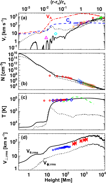
Figure 3: Global structure of our numerical simulation after the system has reached the quasi-steady state. The black solid line in each panel indicates the mean profile of radial velocity (a), the number density (b), and the temperature (c). The standard deviations are superposed as the dotted lines. The blue dashed and red dash-dotted lines in the panel (a) represents sound and Alfvén speed, respectively. The solid and dotted lines in panel (d) represent the root mean square of the velocity in $\theta$ and $\phi$ direction, respectively. All the mean profiles are averaged over 100 minutes in temporally and taken along the central axis of the flux tube. The superposed symbols in each panel represent the observed values as follows. (a) The purple triangle, He line onboard SOHO/SUMER (Wilhelm et al., 2000). The water blue diamond, Ne${}^{7}+$ line onboard SOHO/SUMER (Wilhelm et al., 2000). The orange asterisks, HI Ly $\alpha$ line onboard SOHO/UVCS (Zangrilli et al., 2002). The blue squares, HI Ly $\alpha$ line onboard SOHO/UVCS (Teriaca et al., 2003). The purple solid bars, HI Ly $\alpha$ line onboard SOHO/UVCS (Antonucci et al., 2000). The red circles, coronagraph on SPARTAN (Habbal et al., 1995). The green pluses, IPS observation with VLBI (Grall et al., 1996). (b) The red circles, the electron density by SOHO/SUMER (Wilhelm et al., 1998). The blue stars, the electron density by SOHO/UVCS (Teriaca et al., 2003). The green triangles, the electron density by SOHO/LASCO (Teriaca et al., 2003). The orange squares, the electron density by SOHO/LASCO (Lamy et al., 1997). (c) The red circles, the electron temperature by SOHO/CDS (Fludra et al., 1999). The blue diamonds, the electron temperature by SOHO/SUMER (Wilhelm et al., 1998). The green dashed line, the electron temperature by SWICS/Ulysses (Ko et al., 1997). (d) The blue circles, the non-thermal broadening of Si VIII by SOHO/SUMER (Wilhelm et al., 1998). The red crosses, the non-thermal broadening of Ly $\alpha$ by SOHO/UVCS.

From $t=0$, the foot point of the flux tube is forced to move according to the prescribed velocity perturbation in $\theta$ direction to drive the Alfvénic disturbances. The system below 20 $r_{\rm s}$ (1.4$\times$10⁴ Mm) has reached a quasi-steady state after several Alfvén crossing times have passed. Since we solved time-dependent MHD equations, all the physical variables like the density and the temperature could be evolved to adjust the boundary condition. We have found that the system has a transonic wind and a thin temperature transition from a cool chromosphere to a hot corona. The reproduction of the transonic wind and the hot corona here is a natural consequence of the propagation and dissipation of Alfvén wave since we do not assume any prescribed heating or acceleration functions. In this section, we will describe the mean structure of our hot coronal wind solution. The dynamic features and the detailed heating mechanisms will be described in section 4 and 6, respectively.

The black solid line in figure 3a shows the radial velocity as a function of height. The radial velocity is taken along the central axis of the flux tube and is temporally averaged over 100 minutes. The dotted line represents the standard deviation at each height. The blue dashed and red dash-dotted lines correspond to the sound speed and Alfvén speed, respectively. The sonic point in our solution is located at $r-r_{\rm s}\approx 2$ $r_{\rm s}$ (1.4$\times$10³ Mm) while the Alfvén point is located at $r-r_{\rm s}\approx 17$ $r_{\rm s}$ (1.2$\times$10⁴ Mm). The symbols superposed on the velocity profile represent the observational values. The detailed description of the observations are in the caption of figure 3. The solar wind speed of our model has already reached $\approx$ 600 km s^-1 at 20 $r_{\rm s}$ (1.4$\times$10⁴ Mm), which fairly well agree with the observation.

The temperature and the density profiles are also shown in figure 3b and figure 3c in the similar manner as figure 3a. The sharp transition layer at $r-r_{\rm s}\approx 0.02$ $r_{\rm s}$ (14 Mm) is located bit higher than the observed transition region height above the coronal hole if we regard the observed spicular heights as the transition region height. We shall discuss the detailed dynamics of the transition region in section 4. Since we adopt the electron thermal conductivity that is more efficient than that of protons, the temperature in our model can be regarded as the electron temperature.

The solid and the dotted lines in figure 3d represent the root mean square of $V_{\theta}$ and $V_{\phi}$, respectively. The superposed symbols correspond to the Alfvénic fluctuations inferred from the non-thermal line broadening. The resultant amplitude of $V_{\theta}$ seems to be about twice larger than the observed amplitude. On the other hand, the amplitude of $V_{\phi}$ is significantly smaller than that of $V_{\theta}$ because we impose only Alfvénic fluctuations ($V_{\theta}$) from the photosphere and $V_{\phi}$ is generated through nonlinear mode coupling from the fluctuation in $\theta$ direction. Therefore the expected value of observed velocity ($V_{\rm obs;rms}=[(V_{\theta}^{2}+V_{\phi}^{2})/2]^{-1/2}$) could be reduced to $2^{-1/2}$ of $V_{\rm\theta;rms}$. This effect could be one of the reasons for the discrepancy between the simulated and observed velocity amplitude.

Figure 2a shows the magnetic field structure below 10 Mm ($\sim$1.4$\times 10^{-2}~{}r_{\rm s}$) in the quasi-steady state. The black/gray solid lines represent open/closed magnetic field lines. As is shown in figure 2a, the photosphere and the chromosphere are filled with strong magnetic field so that non-magnetic atmosphere does not exist in our model. Although the flux tube can be deformed according to the resulting gas pressure gradient and the gravity force, the change from the initial potential field is not so large in the present simulation. The iso plasma beta lines are superposed in figure 2a as the dashed lines. Along the central axis of the flux tube, the plasma beta increases from 0.3 at the bottom due to the rapid expansion of the flux tube. The plasma beta ceases to increase at 4.5 Mm with the maximum value of 3 and then decreases with respect to height.

Figure 4 shows the energy flux distribution along the flux tube. The mechanical energy flux that transports the energy outwardly is composed of the following components,

$$F_{\rm alf} \equiv \left({1\over 2}\rho V_{\perp}^{2}+B_{\perp}^{2}\right)V_{r}-\mn@boldsymbol{V_{\perp}}\cdot\mn@boldsymbol{B_{\perp}}B_{r},$$ (71)

$$F_{\rm ent} \equiv {\gamma\over\gamma-1}P_{\rm g}V_{r},$$ (72)

$$F_{\rm knt} \equiv {1\over 2}\rho V_{r}^{3},$$ (73)

$$F_{\rm grv} \equiv -{\rho V_{r}GM\over r},$$ (74)

where $F_{\rm alf},F_{\rm ent},F_{\rm knt}$, and $F_{\rm grv}$ are defined to represent the Alfvénic, enthalpy, kinetic, and gravitational energy flux, respectively. The energy flux in figure 4 is multiplied by the cross section $A$ of the open flux tube. After that, we normalized the energy flux by the cross section $A_{\rm c}$ at the coronal bottom $(r-r_{\rm s}=0.02$ $r_{\rm s}$ or 14 Mm). The Alfvén wave flux is well above $10^{5}$ erg cm^-2 s^-1, a reasonable value to maintain the hot corona (Withbroe & Noyes, 1977). It is found that the Alfvén wave flux dominates the other two energy flux except in two different regions. The enthalpy energy flux becomes comparable to the Alfvén wave energy flux at around $r-r_{\rm s}=0.004$ $r_{\rm s}$ (3 Mm), the region where the flux tube is just opened up. The Alfvénic fluctuation at the photosphere is converted to the enthalpy flux through the linear/nonlinear mode conversion (Matsumoto & Suzuki, 2012). Since the wave amplitude is large below the transition region as shown in figure 5, the efficient nonlinear mode conversion can occur there. The solid, dotted, and dashed lines in figure 5 correspond to $\sqrt{\langle B_{\theta}^{2}\rangle}$,$\sqrt{\langle(B_{r}-\langle B_{r}\rangle)^{2}\rangle}$, and $\sqrt{\langle B_{\phi}^{2}\rangle}$ along the central axis of the flux tube normalized by $\langle B_{r}\rangle$ , respectively. Although our numerical results would idealy be axisymmetric, the perturbations of $B_{\phi}$ appear even along the central axis. This is because the initial magnetic field structure is not perfectly axisymmetric numerically and causes kink motions ($B_{\phi}$) of the flux tube. Above $r-r_{\rm s}\sim 7$ $r_{\rm s}$ (5$\times$10³ Mm), the kinetic energy flux exceeds the Alfvén wave flux. The Alfvén wave pressure pushes the ambient plasma to accelerate the solar wind.

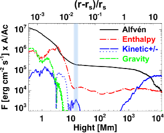
Figure 4: Energy flux in the open field region normalized by the cross section at $r-r_{\rm s}=0.02$ $r_{\rm s}$ (14 Mm). The black (solid), red (dash-dotted), blue (long-dashed(+) or dotted(-)), and green (short-dashed) lines represent the Alfvénic, enthalpy, and kinetic energy, and gravitational energy flux, respectively. Each energy flux is multiplied by the cross section $A$ of the open flux tube, and normalized by the cross section $A_{\rm c}$ at the coronal bottom $(r-r_{\rm s}=0.02$ $r_{\rm s}$ or 14 Mm). The blue shaded area corresponds to the transition region.

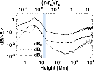
Figure 5: Nonlinearity of magnetic field disturbance along the central axis of the flux tube with respect to height. The solid, dotted, and dashed lines correspond to $\sqrt{\langle B_{\theta}^{2}\rangle}$,$\sqrt{\langle(B_{r}-\langle B_{r}\rangle)^{2}\rangle}$, and $\sqrt{\langle B_{\phi}^{2}\rangle}$ normalized by $\langle B_{r}\rangle$, respectively. The blue shaded area corresponds to the transition region.

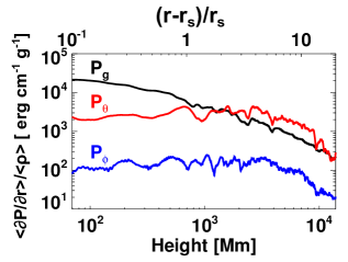
Figure 6: Pressure gradient force per unit mass as a function of height. The black, red, and blue lines represent the contribution from gas pressure ($P_{g}$), and wave pressure ($P_{\theta,\phi}=B_{\theta,\phi}^{2}/2$), respectively. The profiles are averaged over 100 minutes temporally and over $r=r\pm 0.1r$ spatially.

The solar wind in our simulation is accelerated by the wave pressure in addition to the gas pressure. Figure 6 reveals the pressure gradient force with respect to height. The contribution from the gas pressure ($P_{g}$), and the wave pressure ($P_{\theta,\phi}=B_{\theta,\phi}^{2}/2$) is plotted as the black, red, and blue solid lines. Above the sonic point ($r-r_{\rm s}>2$ $r_{\rm s}$ or 1.4$\times$10³ Mm), the contribution from the wave pressure ($P_{\theta}$) exceeds that from the gas pressure ($P_{g}$). Then at around the Alfvén point ($r-r_{\rm s}\approx 17$ $r_{\rm s}$ or 1.2$\times$10⁴ Mm), the contributions from $P_{g}$ and $P_{\theta}$ become comparable again. The $\phi$ component of the wave pressure ($P_{\phi}$) is always less effective than the other two components.

4 Dynamic features

In this section, we shall describe the dynamic features in our simulation. Before going into the detailed discussion, the terminology of the wave mode and the linear property of our model should be clarified. Since $B_{\theta}$ averaged over time is nearly zero everywhere, $(V_{\theta},B_{\theta})$ and the other variables ($\rho,P_{g},V_{r,\phi},B_{r,\phi}$) are almost decoupled within linear theory. We shall call any perturbations of $V_{\theta},B_{\theta}$ as the Alfvénic component. Perturbation of $\rho,P_{g},V_{r,\phi},B_{r,\phi}$ are referred to as the compressible component. The compressible component could be decomposed into slow and fast mode and they can be coupled each other even in linear theory in a non-uniform medium. (e.g. Bogdan et al., 2003). In our simulation, the coupling between the Alfvénic and the compressible component should be nonlinear one that is due to the wave pressure, or ponderomotive force (e.g. Thurgood & McLaughlin, 2013).

4.1 Dynamics below the transition region

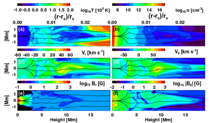
Figure 7: Snapshot images of our simulation after the system has reached the quasi steady state. The background colors indicate the temperature (a), the number density (b), the radial velocity (c), $V_{\theta}$ (d), the radial magnetic strength (e), and the absolute value of the $B_{\theta}$ (f). The black lines in each panel represent the magnetic field lines. Only the open field lines are shown here.

Figure 7 (video available online, movie 1) shows the snapshot images of the temperature (a), the number density (b), the radial velocity (c), $V_{\theta}$ (d), the radial magnetic field strength (e), and $|B_{\theta}|$ (f). The black lines in each panel represent the magnetic field lines projected onto $r-\phi$ plane. Note that the aspect ratio is not correctly displayed in this figure.

Although the prescribed Alfvénic perturbation is uniform in $\phi$ direction, the structures of the higher atmosphere are significantly inhomogeneous in $\phi$ direction. This is mainly because of the inhomogeneity in the magnetic field. The Alfvén speed along the central axis of the flux tube is generally larger than its surroundings. Even when the initial Alfvén wave front is straight in $\phi$ direction, the central part of the wave front tends to propagate faster than the off axis part. This leads to the curved wedge or convex shape of the Alfvén wave front, as was demonstrated by Cargill et al. (1997). This inhomogeneous Alfvénic disturbance creates the radial velocity through the nonlinear mode conversion (e.g. Hollweg et al., 1982), resulting in the inhomogeneity in the density and the temperature.

4.2 Time distance diagram from Photosphere to Low Corona

In order to understand the wave propagation and its interaction with the transition region, time distance diagrams are convenient. Here we focus on dynamic features below 30Mm (4.3$\times$10^-2 $r_{\rm s}$) from the photosphere. Figure 8 represents time distance diagrams of the number density (a), the Alfvén wave nonlinearity or $B_{\theta}/B_{r}$ (b), the radial velocity (c), and $V_{\theta}$ (d). We took the values along the central axis of the flux tube as the horizontal axis and stack the time variance of them onto the vertical axis. The white solid line in each panel corresponds to the transition region height where the temperature is 10⁵K. The white dotted line in each panel indicates the height just above the magnetic canopy averaged over 100 minutes. We can observe a lot of oblique signatures of wave propagation whose inclinations correspond to phase speed. The phase speed increases both in compressible (panels a & c) and Alfvénic (panels b & d) fluctuations at the transition region. However, only the phase speed in Alfvénic fluctuations increases just above the magnetic canopy. Since the super radial decrease in the magnetic field strength is suppressed just above the canopy by the surrounding flux tubes, Alfvén speed increases exponentially according to the decrease in the mass density.

The transition region height exhibits up-and-down motions. Many authors suggest the similarity between these motions and the solar spicules (Hollweg et al., 1982; Kudoh & Shibata, 1999). In figure 8c, we have at least 4 ascending motions of the transition region indicated by white arrows. The ascending events indicated by the solid arrows are associated with upward velocity. This upward velocity originates from fast shocks that could be driven by the nonlinear steepening of Alfvén waves. In low beta plasma such as the chromosphere (around the height of 10 Mm or 1.4$\times$10^-2 $r_{\rm s}$) in our simulation, the nonlinear Alfvén waves produce switch-on shocks as well as slow mode waves. This switch-on shocks lift up the transition region. The daughter slow mode waves can also steepen into shocks due to the gravitational stratification although we can not see the ascending events due to the slow shocks in this time span.

The ascending event indicated by the dotted arrows are not associated with upward velocity. This is just an apparent motion due to the swaying motion of the transition region. We took the time distance diagram along the axis of the flux tube. The transition region is lifted by the fast shock (FS2 in figure 8c) that makes the transition region wedged shape which is similar to the shape shown in figure 7a. The wedged shape transition region reveals swaying motion in $\phi$ direction. If the swaying motion is so large we can see the apparent up-and-down motion of the transition region in the time distance diagram.

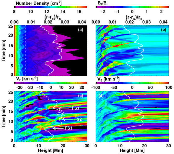
Figure 8: Time distance diagram along the central axis of the flux tube below 30 Mm. The background colors in each panel indicate the number density (a), the Alfvén wave nonlinearity ($B_{\theta}/B_{r}$) (b), the radial velocity (c), and $V_{\theta}$ (d). The white solid line in each panel represents the transition layer where the temperature is 10⁵K. The white dotted line in each panel indicates the height just above the magnetic canopy averaged over 100 minutes. FSs with solid arrows in the panel (c) indicate the collision events between the fast shock and the transition region. FS with dotted arrow in the panel (c) corresponds to the swaying motion of the transition region.

4.3 Time distance diagram from Corona to Solar Wind

Here we focus on wave phenomena up to 15 $r_{\rm s}$ (1.0 $\times$ 10⁴ Mm). Figure 9 shows the time distance diagrams along the central axis of the flux tube below 15 $r_{\rm s}$ (1.0 $\times$ 10⁴ Mm). The radial velocity, $V_{r}-\langle V_{r}\rangle$ (a), the density, $(\rho-\langle\rho\rangle)/\langle\rho\rangle$ (b), $B_{\theta}/\langle B_{r}\rangle$ (c), and $V_{\theta}$ (d) are plotted as contours when the values exceed a certain threshold. The thresholds are $\pm$ 60 km s^-1 (a), $\pm$ 0.25 (b), $\pm$ 180 km s^-1(c), and $\pm$ 0.1 (d). The average operator $\langle\rangle$ here means temporal average over 100 minutes. The mean phase velocity, $V_{r},V_{r}\pm C_{\rm s},V_{r}\pm V_{A}$ are plotted as arrows on the top of the panel as references.

The propagating signature in the radial velocity and the density fluctuations in figure 9 corresponds to compressible waves. From the slope of the signature, these compressible waves are considered to be slow mode waves. There are several origin of the slow mode wave in the corona. In the chromosphere, the nonlinear steepening of Alfvén waves produces the switch-on (fast) shocks. When the switch-on shocks enter the corona they creat slow mode shocks as well as fast shocks. The nonlinear mode conversion or the parametric decay of the Alfvén waves in the corona can also be the origin of the slow mode waves since the nonlinearity of the Alfvén waves is not so small (0.1-0.2) in the corona (Fig. 5). The density fluctuation reaches $\approx$ 0.8 on average at $r=10$ $r_{\rm s}$ (7.0 $\times$ 10³ Mm) and sometimes exceeds unity. The fluctuation in Alfvén speed due to the density fluctuation could be the reflection source of the Alfvén waves.

The figure 9c and 9d represents the propagation of the Alfvén waves. Besides the out going Alfvén waves, the signatures of reflected waves can be seen as the dotted lines in the figure 9d. This is due to the density fluctuation by the slow mode waves and to the gradual change in the background Alfvén speed (Suzuki & Inutsuka, 2005, 2006). The reflection of Alfvén waves are important in the context of the solar wind turbulence. The wave-wave interaction between out and in going Alfvén waves are considered to trigger the nonlinear cascade of MHD turbulence (Matthaeus et al., 1999). Although MS12 suggested that the anisotropic cascade can be seen in their simulation, improving the radial grid size removed the signature of the cascade. We probably need full 3 dimensional simulations to describe the nonlinear wave-wave interaction (van Ballegooijen et al., 2011).

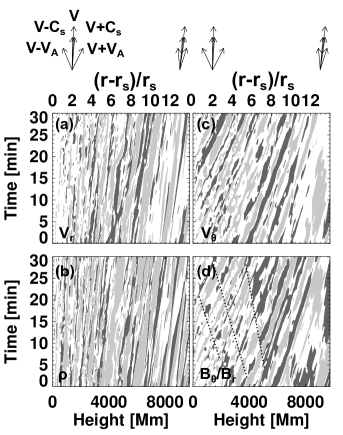
Figure 9: Time distance diagram along the central axis of the flux tube below 15 $r_{\rm s}$ (1.0 $\times$ 10⁴ Mm). (a) The variations of the radial velocity, $V_{r}-\langle V_{r}\rangle,$ that exceed the threshold of +/- 60 km s^-1 are shown in dark/light contours. (b) The relative variations of the density, $(\rho-\langle\rho\rangle)/\langle\rho\rangle$. The thresholds are +/- 0.25. (c) The variations of $V_{\theta}$. The thresholds are +/- 180 km s^-1. (d) The relative variations of $B_{\theta}/\langle B_{r}\rangle$. The thresholds are +/- 0.1. The dotted lines corresponds to the signature of reflection waves. The mean phase velocity, $V_{r},V_{r}\pm C_{\rm s},V_{r}\pm V_{A}$ are plotted as arrows on the top of the panel as references.

5 Data Analysis

Before investigating heating mechanisms that actually work in our model, we should describe how to estimate the heating rate. Since we do not have any explicit viscosity and resistivity in our basic equations, the estimation of the heating rate is not so straightforward task. Inclusion of explicit dissipation terms will help us to estimate the heating rate although it will smooth out large scale structures as well as small scale structures. Hyper diffusion method will keep large scale structures sharp while appropriate dissipation is introduced in small scale (Rappazzo et al., 2008; van Ballegooijen et al., 2011). However, the appropriate diffusion coefficients may vary as a function of grid size and typical velocity such as Alfvén and sound speed, it is not straightforward to choose the functional form of the diffusion coefficients. Therefore instead of using hyper diffusion, we simply choose not to use explicit dissipation terms as a first step, although the estimation of heating rate will be more complicated and less rigorous.

In this section, we briefly explain the idea to estimate the total heating rate. Basically there are two kinds of dissipation in numerical simulations without explicit physical dissipation terms. The first one is physical dissipation associated with shocks. This dissipation is introduced when Riemann solver is used for flux estimation while the artificial viscosity may be used for other methods. The second one is numerical dissipation associated with truncation errors. Advection of shear flows or magnetic shear could cause the numerical dissipation. This type of dissipation is not always physical dissipation especially when the numerical resolution is very poor. This type of numerical dissipation could be regarded as the physical one if there is the physical reason for small scale cascading such as turbulence.

For an illustrative purpose, we here explain our method to measure the heating rate in the 1.5 MHD in Cartesian coordinate system without thermal conduction and radiative cooling as a simplest example. The 1.5 dimensional system here means the system that has spatial variation only in $x$ direction but has vector component in $y$ direction in addition to $x$ direction. Please see appendix B for the actual method we are performing in our spherical 2.5D MHD system.

Since we use the finite volume method, the internal energy $u$ will be calculated after all the conservative variables are updated. Then the discretized form of the time derivative of $u$ can be written down as follows.

$${u^{n+1}_{i}-u^{n}_{i}\over\Delta t}={E^{n+1}_{i}-E^{n}_{i}\over\Delta t}-{1\over\Delta t}\left\{{(M^{n+1}_{i})^{2}\over 2\rho^{n+1}_{i}}-{(M^{n}_{i})^{2}\over 2\rho^{n}_{i}}\right\}-{1\over\Delta t}\left\{{(B^{n+1}_{i})^{2}\over 2}-{(B^{n}_{i})^{2}\over 2}\right\},$$ (75)

where $i$ and $n$ indicate the spatial and the temporal index, respectively. The momentum in Cartesian coordinate system, $M_{x,y}$, corresponds to ${\cal M}_{r,\phi}$ in eq (18) and defined to be $\rho V_{x,y}$. If we transform the time differences of the conservative variables on the right hand side of eq (75) to the spatial differences of the corresponding flux,

$${u^{n+1}_{i}-u^{n}_{i}\over\Delta t} = Q_{n;i}+Q_{a;i},$$ (76)

where

$$Q_{n;i} = -\Delta_{x}\left\{(u+P_{g})V_{x}\right\}+{M^{n+1/2}_{x;i}\over\rho^{n+1}_{i}}\Delta_{x}P_{g}$$ (77)

and

$$Q_{a;i} = {M^{n+1/2}_{x;i}\over\rho^{n+1}_{i}}\Delta_{x}\left(\rho V_{x}^{2}\right)+{M^{n+1/2}_{y;i}\over\rho^{n+1}_{i}}\Delta_{x}\left(\rho V_{x}V_{y}\right)$$ (78)

$$- {(M^{n}_{i})^{2}\over 2\rho^{n}_{i}\rho^{n+1}_{i}}\Delta_{x}\left(\rho V_{x}\right)-\Delta_{x}\left({1\over 2}\rho V^{2}V_{x}\right)$$

$$+ {M^{n+1/2}_{x;i}\over\rho^{n+1}_{i}}\Delta_{x}{B_{y}^{2}\over 2}-{M^{n+1/2}_{y;i}\over\rho^{n+1}_{i}}\Delta_{x}{B_{x}B_{y}}$$

$$- B_{y;i}^{n+1/2}\Delta_{x}\left(B_{x}V_{y}-B_{y}V_{x}\right)-\Delta_{x}\left(B_{y}^{2}V_{x}-V_{y}B_{y}B_{x}\right).$$

The spatial difference are defined as $\Delta_{x}f\equiv(f^{*}_{i+1/2}-f^{*}_{i-1/2})/\Delta x_{i}$ and the asterisk on $f$ indicate the variables at the cell surface estimated by the approximate Riemann solver. $f^{n+1/2}_{i}$ is defined to be $(f^{n+1}_{i}+f^{n}_{i})/2$ for arbitral variable $f$. Note that $B_{x}$ is constant in 1D Cartesian case and can be removed from inside the difference. The first term in eq (76), $Q_{n}$, is generally non zero term and roughly corresponds to the discretized form of the adiabatic expansion (-$\gamma u\partial u/\partial x$) plus the advection ($-V_{x}\partial u/\partial x$). This term, however, is slightly different from the adiabatic expansion and advection term since the numerical flux used in the spatial difference may implicitly have dissipative component originated from the (approximate) Riemann solver. The second term in eq (76), $Q_{a}$, should analytically equal to zero when we replace the spatial difference with the spatial derivative. However, discretizing operation leads $Q_{a}$ to have some residual values that we consider contribute partly to the numerical dissipation. $Q_{n}$ roughly corresponds to the sum of adiabatic heating and heating at hydrodynamical shocks, while $Q_{a}$ consists of the rest of all the entropy generation, the sum of numerical viscous dissipation by velocity shear and numerical resistive dissipation of magnetic field.

Test simulations in appendix B suggests that $Q_{a}$ always gives good estimation for Alfvén waves while $Q_{a}$ is good indicator for fast waves only in low beta plasma. For slow waves, $Q_{a}$ always underestimates numerical dissipation significantly and the dissipation mainly originates from $Q_{n}$.

Generally $\langle Q_{n}\rangle$ can be divided into two components. The first one is organized only by bulk variables such as $\langle u\rangle$, $\langle P\rangle$, $\langle V_{\rm x}\rangle$. This component could be considered as the adiabatic loss due to the solar wind expansion. The second one is organized by the cross correlation between fluctuations in $u,P,V_{\rm x}$. This component possibly originates from the heating due to acoustic and shock waves. Accordingly, the solar wind loss component ($Q_{\rm WL}$) and the acoustic and shock wave component ($Q_{\rm AS}$) can be described as follows.

$$Q_{\rm WL} \equiv -{\partial\over\partial x}\left\{(\langle u\rangle+\langle P_{g}\rangle)\langle V_{\rm x}\rangle\right)+\langle V_{x}\rangle\langle{\partial P_{g}\over\partial x}\rangle,$$ (79)

$$Q_{\rm AS} \equiv \langle Q_{n}\rangle-Q_{\rm WL}.$$ (80)

Note that $Q_{\rm WL}$ and $Q_{\rm AS}$ are the temporally averaged value while $Q_{n}$ and $Q_{a}$ are the functions of time.

6 Heating Rates

In section 5, we describe the idea to precisely measure the heating rate that actually occurred in our simulation. Figure 10 represents the energy balance with respect to height. All the heating rates below are averaged over 100 minutes temporally and over all $\phi$ domain spatially. Moreover, the heating rates are spatially averaged over $0.8(r-r_{\rm s})<r-r_{\rm s}<1.2(r-r_{\rm s})$. The black solid line with diamonds corresponds to $Q_{a}$ averaged over time and space. The green solid/dashed line with squares indicates the conduction heating/loss while the blue dashed line with triangles shows the radiation loss. $Q_{\rm AS}$ is represented by the red solid line with asterisks while the solar wind loss or $-Q_{\rm WL}$ is denoted by the purple dashed line with pluses. Below the transition region ($r-r_{\rm s}<0.02$ $r_{\rm s}$ or 14 Mm), the radiative loss is balanced by the sum of $Q_{\rm AS}$ and $Q_{a}$, or mechanical heating rate. Around the transition region ($r-r_{\rm s}\approx 0.02$ $r_{\rm s}$ or 14 Mm), the contribution of the thermal conductive heating becomes significant as well as the radiation and the mechanical heating. The sudden increase in temperature profile causes the strong increase of the thermal conductive heating here. At the coronal bottom $r-r_{\rm s}\approx 0.05$ $r_{\rm s}$ (35 Mm), the thermal conductive loss and the solar wind loss are balanced by the mechanical heating rate and the radiative cooling becomes negligible. In the solar wind acceleration region ($r-r_{\rm s}>r_{\rm s}$ or 700 Mm), the thermal conduction loss is balanced by $Q_{a}$.

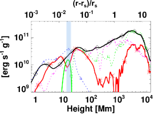
Figure 10: Energy balance after the system has reached the quasi-steady state. The black (with diamonds), green (with squares), blue (with triangles) , red (with asterisks), and purple (with pluses) lines correspond to the $Q_{a}$, the thermal conduction, the radiative loss, $Q_{\rm AS}$ and the adiabatic loss due to the solar wind ($Q_{\rm WL}$), respectively. All the heating/cooling rates are normalized by $\langle\rho\rangle$ in this plot. The solid lines indicate the positive value (heating) while the dotted lines indicate the negative value (cooling). The blue shaded area corresponds to the transition region.

6.1 Heating below the transition region

The mean profiles of the heating rate clearly show that the heating events below the transition region are dominated by $Q_{a}$ and $Q_{\rm AS}$ (fig 10). Combining the mean heating profiles and the snapshot images of the total heating rate, we found that the dominant heating mechanism below the transition region was shock heating. Figure 11 (video available online, movie2) shows the snapshot images of $Q_{a}/\langle\rho\rangle$ (a), the squared current density over the mass density (b), the velocity convergence ($\nabla\cdot v<0$) (c), and $V_{\theta}$ (d). The spatial distribution and the time evolution of the heating rate tell us what is the actual heating mechanisms in our numerical simulation. There is a shock (FS in figure 11b) propagating toward right hand side. At the down stream of the shock, the magnetic pressure ($B_{\theta}^{2}/2$) increases. From this property, we identified FS as a fast shock. The location of FS corresponds to the region where the heating rate ($Q_{a}$) is significantly high. The locations with converging motion ($\nabla\cdot v<0$) tend to have high $Q_{a}$ in the chromosphere, which means the chromospheric shocks are well captured by $Q_{a}$. We also have high $Q_{a}$ region without conversing motion probably because of the low numerical resolution. At most 2/3 of $Q_{a}$ comes from the shock region in the chromosphere (fig 13a), although the ratio will be smaller in higher numerical resolution. The contribution of the slow shocks could be important as well. There are also a lot of switch off slow shocks in our simulation, for example SS in figure 11b. Instead of the swith off shocks, the switch on fast shocks will appear at the higher height where the background plasma beta is low. As was discussed by Hollweg (1982), the fast switch on shocks are one of the main mechanisms in our simulation in the higer chromosphere. We think both the fast and slow shocks are important heating mechanisms in our simulation, although we have not yet elucidated which is more important statistically.

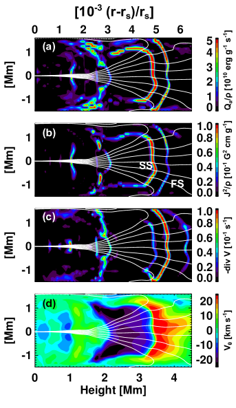
Figure 11: Heating events around the chromosphere. The color contours represent $Q_{a}/\langle\rho\rangle$ (a), the current density square per unit mass (b), the velocity convergence ($\nabla\cdot v<0$) (c), and $V_{\theta}$ (d). The white lines in each panel indicate the magnetic field lines.

6.2 Heating just above the transition region

The heating mechanism just above the transition region is different from that below the transition region. Figure 12 shows the temporal evolution of a typical heating event just above the transition region (video available online, movie 3). From the left to the right column, $Q_{a}/\langle\rho\rangle$, the squared current density per unit mass, and $V_{\theta}$ are shown. Time goes on from the top to the bottom with 18 second temporal intervals. The transition region is indicated by the thick white lines and is significantly deformed due to collisions with shocks.

In the first row of figure 12, an Alfvén wave front comes from the left hand side. The injected Alfvén wave has already been nonlinearly steepened into the fast shock to have small length scale in radial direction before they collide with the transition region. The steepening in radial direction creates the current density in $\phi$ direction along the wave front as was seen in the first row of figure 12. Between $t=0$ and $t=+18$, the fast shock collides with the transition region. The shock front refracts significantly because of the huge difference in phase speed across the transition region. When the chromospheric fast shock hits the transition region, the chromospheric fast shock would split into an out-going fast/slow shock, a contact discontinuity ( can be seen as spicules ) and an in-going fast rarefaction wave. Since the Mach numbers of the fast shock are so small that we could not see the shocks clearly. In addition, we have an out-going Alfvén wave between the fast and slow shock. The resultant Alfvén wave has an elongated wedge shape structure shown in figure 12c. We do not detect velocity convergence ($\nabla\cdot v<0$) along the wedge shape structure, which means this structure is not the shock but some kind of Alfvén waves. The Alfvén wave has large current density along the wave front that can be dissipated to heat the coronal bottom.

The concave structure of the transition region can also be important because it produces the steep gradient of Alfvén speed not only in vertical direction but also in horizontal direction. The strong inhomogeneity in horizontal direction can proceed the so called phase mixing of Alfvén waves (Heyvaerts & Priest, 1983). We think the phase mixing just above the transition region stimulates the coronal heating in our simulation.

The acoustic heating rate is also important at $r-r_{\rm s}\approx 0.04$ $r_{\rm s}$ (30 Mm) The acoustic heating originates from the shock waves that are formed in the chromosphere and injected to the coronal bottom (Hollweg, 1982).

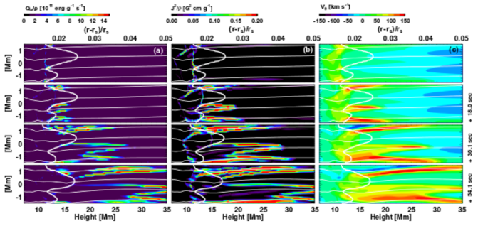
Figure 12: Time series of a collision event between an Alfvén wave and the transition region. The left (a), middle (b), and right (c) column represent $Q_{a}/\langle\rho\rangle$ , the current density square per unit mass, and $V_{\theta}$, respectively. The thin white lines indicate the magnetic field lines. The thick white line in each panel shows the transition layer where the temperature is 10⁵ K.

6.3 Heating in the solar wind acceleration region

In the solar wind acceleration region ($r-r_{\rm s}>r_{\rm s}$ or 7$\times$10² Mm), incompressible heating mechanisms are dominant. The incompressible heating mechanism here means the mechanisms such as MHD turbulence or phase mixing. Figure 13a shows that the incompressible component dominates the compressible component. The compressible component is derived in the way that we sum up $Q_{a}$ over the region where the velocity divergence is negative. The rest of $Q_{a}$ is referred to as the incompressible component. The incompressible component exceeds the compressible component above $r-r_{\rm s}=0.03$ $r_{\rm s}$ (21 Mm). Therefore the plasma heating in the solar wind are dissipation of magnetic energy through incompressible process, although the heating is done through numerical dissipation.

Extension to 3D could be essential in terms of the property of MHD turbulence in the solar wind. Reduced MHD that excludes the compressibility from the usual MHD is useful approach for MHD turbulence in the solar wind and extensive studies have been done in the reduced MHD formulation so far (Matthaeus et al., 1999; Dmitruk & Matthaeus, 2003; Verdini & Velli, 2007; van Ballegooijen et al., 2011). Although the compressibility turns out not to contribute the total heating rate directly, it produces large density fluctuations that could change the reflection rate of Alfvén waves. Since the efficiency of MHD turbulence depends on the amount of the reflection waves, the compressibility could affect the total heating rate indirectly.

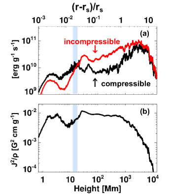
Figure 13: Comparison between compressible and incompressible components of magnetic heating rate as a function of height (a), and mean profile of current density per unit mass (b). The black/red solid line in panel (a) corresponds to compressible/incompressible heating rate. The blue shaded area corresponds to the transition region.

7 Discussions

Thanks to the new analysis method described in section 5 and appendix B, we can derive more accurate profile of the heating rate than that was reported by MS12. Although the numerical simulation shown here is almost the same as that of MS12, the new analysis method and higher numerical resolution lead us two different interpretations about heating mechanisms in the corona.

First, MS12 suggested that the shock dissipation and MHD turbulence are the main heating mechanisms at the coronal bottom. We concluded that, instead of MHD turbulence, Alfvén waves with curved wedge shape originate from the chromospheric fast shocks is main heating mechanisms at the coronal bottom. Phase mixing due to the concave transition region may also stimulate the coronal heating. The heating rate derived in this paper is more reliable than that of MS12. Next, MS12 suggested that MHD turbulence is the dominant heating mechanisms in the solar wind. The finer radial resolution reveals that we do not achieve the shallower power spectrum like Kolmogorov-type turbulence. We confirm that the magnetic energy are converted to the thermal energy through incompressible processes, although it is difficult to distinguish what kind of heating mechanisms operate in the solar wind.

We derive heating rate in our numerical simulation that inevitably has numerical dissipation larger than that of the realistic solar atmosphere. Therefore we should discuss the validity or the robustness of the heating mechanisms found in our simulations, although we do need further numerical experiments to investigate whether our results depend on numerical resolution. Shock heating rate would not depend on the grid size and microscopic physics like viscosity or resistivity as far as Rankine-Hugoniot relations are satisfied. Since our numerical scheme (HLLD scheme) is conservative and meditated to capture MHD shocks, the shock heating in our numerical simulation should not be just a numerical heating but a physical one.

Heating events at the coronal bottom are associated with curved wedge shape structure described in section 6. This structure would be Alfvén wave front with large current density that was stored in the chromospheric fast shocks. Whether this structure keeps large current density or not might depend on the numerical resolution. The dynamic simulations with high resolution are needed to justify this heating mechanism.

The heating by phase mixing depends on viscosity or resistivity so that our results could be affected by numerical resolution. The phase mixing in our simulation turns on because of the horizontal phase speed difference that is created by the collision between the transition region and shock waves. Then the duration that phase mixing operates is finite and determined by the Alfvén crossing time between peaks and troughs of the transition region. The finite duration for phase mixing results in the finite thickness of the current density. Therefore this will prevent phase mixing from cascading to the dissipation scale that is determined by microscopic physics, although, in our simulation, Alfvén waves dissipate due to insufficient grid numbers in $\phi$ direction. Therefore there is a possibility that the phase mixing discussed here may be weaken to operate if we increase grid numbers. Extension to 3 dimensional simulation could stimulate phase mixing by increasing the effective viscosity or resistivity through instability due to velocity or magnetic field shear. Or inhomogeneity in $\theta$ direction makes phase mixing less effective as was suggested by Parker (1991).

In the present study, we only consider shear Alfvén fluctuations ($V_{\theta}$) as the energy injection from the photosphere. However the realistic fluctuations would also be associated with kink and torsional types in the complex solar atmosphere without translational symmetry ($\partial_{\theta}=0$). Torsional Alfvén waves could be generated by the vortex flows observed in the photosphere (Brandt et al., 1988), and the connection between the vortex flows and swirling motions in the upper atmosphere are observed recently (Wedemeyer-Böhm et al., 2012). Since the difference in nonlinear behaviors between torsional and shear mode is discussed by Vasheghani Farahani et al. (2011), dynamic behaviors could be affected if we include torsional Alfvén waves. This aspect will be explored in future work by using axisymetric 2.5 dimensional simulations or full 3 dimensional simulations.

Since we only prescribe Alfvénic fluctuations that cannot be linearly converted into compressible mode, the nonlinear development of Alfvén waves is important to heat the atmosphere. The wave nonlinearity $V_{\theta}/V_{\rm A}$ is proportional to $\rho^{1/4}B^{-1}$ if we consider the wave energy flux conservation in an static atmosphere, $\rho V_{\theta}^{2}V_{\rm A}A=$ const, where $A$ is the cross section of the flux tube. This means that not only the density structure but also the expansion rate of the magnetic field are important for the development of the wave nonlinearity. The previous 1 dimensional simulations artificially defined the cross section of flux tubes. The magnetic field in our model has nearly the potential field structure similar to that in Bogdan et al. (2003), which makes our simulation more realistic than the 1 dimensional simulations. Our model, however, cannot describe the non-magnetic atmosphere below the magnetic canopy, since potential field structure needs the surrounding magnetic pressure to support the strong magnetic flux tube. For more realistic simulation, we should implement the magnetohydrostatic atmosphere in the similar way Hasan et al. (2005) did to investigate the compressible wave propagation.

From the chromospheric observations with HINODE/SOT, de Pontieu et al. (2007) suggested that there are two types of spicules: Type I spicules exhibit up-and-down motion and have relatively slow ascending speed while Type II spicules fade out and often have high speed upward motion larger than 100 km s^-1. If we regard the up-and-down motion of the transition region as spicules, the radial velocity of our spicules is usually 60 km s^-1 at most. Therefore the collision between shock waves and the transition region could not lift up the plasma so rapidly as Type II spicules do and other mechanisms will be needed (e.g. Martínez-Sykora et al., 2011). It should be noted however that the existence of the Type II spicules is still under debate so far (Zhang et al., 2012; Pereira et al., 2012).

8 Summary

We have implemented a 2.5 dimensional MHD simulation that resolves the propagation and the dissipation of the Alfvén waves in the solar atmosphere. The hot corona and the high speed solar wind are reproduced as a natural consequence of the Alfvén wave injection from the photosphere, as was shown in MS12. However, the detailed analysis of the heating rate leads us to the different interpletation as follows.

• Alfvén waves with curved wedge shape generated by the chromospheric fast shocks heat the coronal bottom while MS12 suggested heating by MHD turbulence.

• Anisotropic turbulent cascade that was found in the simulation of MS12 turned out to disappear when increasing radial resolution. The heating in the solar wind operates through the magnetic energy conversion with incompressible process, though we could not distinguish the specific heating mechanisms so far.

Appendix A Resolution Test

In order to check the dependence of our results on the numerical resolution, we have performed high resolution runs. Since we do not have enough CPU power, we will measure the energy flux at the corona resulting from a sinusoidal Alfvénic fluctuation at the photosphere. For simplicity, we ignore the radiation cooling and thermal conduction. Initial magnetic field is the same as the one described in section 2. As for temperature distribution, we set a tangent hyperbolic function,

$$T=T_{0}+{1\over 2}(T_{c}-T_{0})(1+\tanh{{x-h\over w}}),$$ (81)

to mimic the photosphere, transition region, and corona, where $T_{0}=6,000$ K, $T_{c}=2$ MK, $x$ is height, $h=3,000$ km, and $w=500$ km. The photospheric density is set to be $10^{-7}$ g cm^-3 and the hydrostatic equation is solved to get the density stratification.

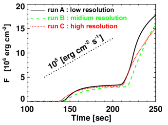
Figure 14: Accumulated Poynting flux at 10 Mm (see eq 83 in text) as a function of time. The black solid, green dashed, and red dotted lines represent the results from run A (low resolution), run B (medium resolution), and run C (high resolution). The slope of the dotted line corresponds to the energy flux of 10⁵ erg cm^-2 s^-1.

Alfvén wave is driven by specifying a sinusoidal velocity perturbation,

$$V_{\theta}=2\sin{{2\pi t\over 180{\rm~{}sec}}}{\rm~{}km~{}s^{-1}}.$$ (82)

The velocity perturbation is set to be zero when $t>180$ sec. Three simulations have been performed, changing the grid number shown in table 1. The mesh sizes are constant below 10 Mm. The vertical mesh sizes are enlarged above 10 Mm so that the maximum height is greater than 800 Mm.

Figure 14 shows the Poynting flux averaged over $\phi$ and integrated over time at 10 Mm,

$$F\equiv{1\over\Delta\phi}\int_{\Delta\phi}d\phi\int_{0}^{t}-B_{\theta}V_{\theta}B_{r}dt^{\prime},$$ (83)

where we just pick up the contribution from $\theta$ component that is larger than the other components. During $140<t<210$ sec, the first half of the injected sinusoidal wave passed, while the second half of the wave passed after $t=210$ sec. As long as the Poynting flux is concerned, the relative error in this simulation is less than 50 %.

	grid number	grid size [km] ∗
run A	2048x32	25x93.8
run B	2048x128	25x23.4
run C	4096x512	6.1x5.9

Table 1: ^∗ This grid size is measured below 10 Mm. Above 10Mm, the vertical grid size is enlarged.

Appendix B Estimation of heating rate

In section 5, we gave the basic idea to estimate the heating rate. We will describe the detailed numerical procedure in this appendix. The method can be applied to the numerical scheme that uses the finite volume method with some kind of Riemann solver flux estimation. Although the description here is for 2.5 dimensional spherical coordinate system, application for the other orthogonal coordinate system is straightforward.

In the finite volume method, internal energy is updated after all the other conservative variables are updated. Then the discretized equation for internal energy update will be

$$\Delta ur^{2}=\Delta{\cal E}-\Delta{\rho V^{2}r^{2}\over 2}-\Delta{B^{2}r^{2}\over 2},$$ (84)

where $\Delta f\equiv(f_{i,j}^{n+1}-f_{i,j}^{n})/\Delta t$ and $f$ is arbitrary variable, and ${\cal E}=r^{2}E$. The superscript indicates a certain time step $n$ and the subscripts $i$ and $j$ represent the discretized index of the spatial coordinate $r$ and $\phi$, respectively. $\Delta t$ represents the time interval between the time step $n$ and $n+1$.

The change rate of the kinetic energy can be decomposed into several parts within the rounding error as follows.

$$\Delta{\rho V^{2}r^{2}\over 2} = {1\over\Delta t}\left[{\left({\cal M}^{n+1}\right)^{2}\over 2{\cal R}^{n+1}}-{\left({\cal M}^{n}\right)^{2}\over 2{\cal R}^{n}}\right]$$ (85)

$$= \sum_{\alpha=r,\theta,\phi}{{\cal M}^{n+1/2}_{\alpha}\Delta{\cal M}_{\alpha}\over{\cal R}^{n+1}}-{\left({\cal M}^{n}_{\alpha}\right)^{2}\Delta{\cal R}\over 2{\cal R}^{n+1}{\cal R}^{n}},$$

where $f^{n+1/2}\equiv(f^{n}+f^{n+1})/2$, ${\cal R}=r^{2}\rho$, and ${\cal M}_{\alpha}=r^{2}\rho V_{\alpha}$. In equation (84) and (85), $\Delta{\cal E}$ and $\Delta{\cal M}_{\alpha}$ can be described by the spatial difference of the numerical flux. If we extract the terms related to gas pressure from the spatial difference, the equation (84) can be divided into two parts as was done in section 5, as follows.

$$\Delta u=Q_{n}+Q_{a},$$ (86)

where

$$Q_{n}=-{\Delta_{r}\left[\left(u+P_{g}\right)V_{r}r^{2}\right]\over r_{i}^{2}}-{\Delta_{\phi}\left[\left(u+P_{g}\right)V_{\phi}\right]\over r_{i}}+{{\cal M}_{r;i,j}^{n+1/2}\over{\cal R}_{i,j}^{n+1}r_{i}^{2}}\Delta_{r}\left(P_{g}r^{2}\right)+{{\cal M}_{\phi;i,j}^{n+1/2}\over{\cal R}_{i,j}^{n+1}r_{i}}\Delta_{\phi}\left(P_{g}\right),$$ (87)

where $\Delta_{r}f\equiv(f_{i+1/2,j}^{*}-f_{i-1/2,j}^{*})/\Delta r_{i}$ and $\Delta_{\phi}f\equiv(f_{i,j+1/2}^{*}-f_{i,j-1/2}^{*})/\Delta\phi_{j}$. $Q_{n}$ can roughly be regarded as the sum of adiabatic heating and heating at hydrodynamical shocks, while $Q_{a}$ consists of the rest of all the entropy generation, the sum of numerical viscous dissipation by velocity shear and numerical resistive dissipation of magnetic field. Although $Q_{n}$ may be estimated by the central differences, we found that the positivity of $Q_{a}$ is significantly improved when we use the variables from Riemann solver for the inside of the numerical difference. We can not derive all the variables individually, since HLLD scheme is approximate Riemann solver and can not derive gas pressure self-consistently. Instead, we only know averaged value of $E,P_{T},\mathbf{V},\mathbf{B}$, and $\rho$ at the cell surface in HLLD scheme. Therefore when we use HLLD scheme, we adopt further approximation as follows.

$$P_{g} \equiv P_{T}-{B^{2}\over 2}$$ (88)

$$u+P_{g} \equiv E-{1\over 2}\rho V^{2}+P_{T}-B^{2}$$ (89)

The second term in (86), $Q_{a}$, can be derived if we subtract $Q_{n}$ from $\Delta u$.

B.1 dissipation of linear wave in MHD

In order to investigate the property of $Q_{n}$ and $Q_{a}$, we have performed test simulations for dissipation of linear MHD wave. We use 2D ($x,z$) Cartesian grid with grid numbers of ($N_{x},N_{z}$) = (128, 64). The spatial domain is $(0<x<\sqrt{5})$ and $(0<z<\sqrt{5}/2)$. The initial conditions are described as follows.

$$\mathbf{q}^{\rm initial} = \bar{\mathbf{q}}+\epsilon\mathbf{r}_{k}\sin{2\pi x^{\prime}},$$ (91)

$$x^{\prime} = x\cos{\theta}+z\sin{\theta},$$ (92)

where

$$\mathbf{q} = \left(\rho,V_{\rm x^{\prime}},V_{\rm y^{\prime}},V_{\rm z^{\prime}},B_{\rm x^{\prime}},B_{\rm y^{\prime}},B_{\rm z^{\prime}},P_{g}\right),$$ (93)

$$\bar{\mathbf{q}} = \left(1,0,0,0,B_{0}\cos{\theta_{\rm B}},0,B_{0}\sin{\theta_{\rm B}},1/\gamma\right),$$ (94)

and $\mathbf{r}_{k}$ is the right eigen vectors that are described in subsection B.2. The wave amplitude, $\epsilon$, is set to be $10^{-2}$ and $\theta$ is the angle of the wave number vector measured from $x$ axis where $\tan^{-1}\theta=2$. $\gamma(=5/3)$ is specific heat ratio and $\theta_{\rm B}$ is the angle between the wave number vector and the background magnetic field. Periodic boundary conditions are posed on both boundaries. Although we do not include any explicit dissipation term, total kinetic and magnetic energy will be decreasing by numerical dissipation. We have performed several simulations with different plasma beta and $\theta_{\rm B}$.

Figure 15: Normalized numerical heating rate in linear MHD wave propagation with different plasma beta and $\theta_{\rm B}$ .

For each run, we can measure the energy loss rate of kinetic and magnetic energy averaged over space and time. In the meantime, we can obtain $Q_{a}$ averaged over space and time. The averaging procedures are done over all the spatial domain and over one wave period. Then we can obtain $Q_{a}$ normalized by the energy loss rate for each run. Figure 15a shows the normalized heating rate as a function of $\theta_{\rm B}$ for Alfvén wave with plasma beta equals to $0.1$. Each diamond corresponds to a single run, where the distance between the origin $(O)$ and the diamond $(P)$ indicates normalized heating rate and the angle between the line $\overline{OP}$ and horizontal axis represents $\theta_{\rm B}$. We plotted a unit circle by the dotted line as a reference. Figure 15a suggests that $Q_{a}$ is excellent indicator of numerical dissipation rate for Alfvén wave. The panels b-f of figure 15 corresponds to the runs for fast mode with $\beta=0.1$ (b), slow mode with $\beta=0.1$ (c), Alfvén mode with $\beta=5$ (d), fast mode with $\beta=5$ (c), slow mode with $\beta=5$ (f). This figure suggests that $Q_{a}$ always gives good estimation for Alfvén waves while $Q_{a}$ is good indicator for fast waves only in low beta plasma. For slow waves, $Q_{a}$ always underestimates numerical dissipation and the dissipation mainly originates from $Q_{n}$.

These results suggest that $Q_{a}$ and $Q_{n}$ corresponds to the dissipation rates of magnetic and gaseous energy, respectively. Since the fast waves in high(low) beta plasma have large(small) thermal energy, $Q_{a}$($Q_{n}$) becomes the dominant dissipation term. On the other hand the slow waves in high(low) beta plasma have small(large) thermal energy so that $Q_{a}$($Q_{n}$) has considerable effects on total dissipation.

B.2 eigen vectors

Here we show the right eigen vectors used in the test simulations for linear MHD waves. The right eigen vectors under the background condition of eq 94 can be written as

$${\mathbf{r}}_{\rm f}=\left(\begin{array}[]{c}\alpha_{\rm f}\\ \alpha_{\rm f}c_{\rm f}\\ 0\\ -\alpha_{\rm s}c_{\rm s}\\ 0\\ \alpha_{\rm s}\\ \alpha_{\rm f}\end{array}\right),$$ (102)

$${\mathbf{r}}_{\rm s}=\left(\begin{array}[]{c}\alpha_{\rm s}\\ \alpha_{\rm s}c_{\rm s}\\ 0\\ \alpha_{\rm f}c_{\rm f}\\ 0\\ -\alpha_{\rm f}\\ \alpha_{\rm s}\end{array}\right),$$ (110)

$${\mathbf{r}}_{\rm A}=\left(\begin{array}[]{c}0\\ 0\\ 1\\ 0\\ -1\\ 0\\ 0\end{array}\right),$$ (118)

where $\mathbf{r}_{\rm f}$, $\mathbf{r}_{\rm s}$, and $\mathbf{r}_{\rm A}$ represent the right eigen vectors of fast, slow, and Alfvén wave, respectively and

$$c_{\rm f,s}^{2}={1\over 2}\left[1+V_{\rm A}^{2}\pm\sqrt{\left(1+V_{\rm A}^{2}\right)^{2}-4V_{\rm A}^{2}\cos^{2}{\theta_{\rm B}}}\right],$$ (119)

$$\alpha_{\rm f}^{2} = {1-c_{\rm s}^{2}\over c_{\rm f}^{2}-c_{\rm s}^{2}},$$ (120)

$$\alpha_{\rm s}^{2} = {c_{\rm f}^{2}-1\over c_{\rm f}^{2}-c_{\rm s}^{2}},$$ (121)

where $\alpha_{\rm f/s}$ is defined as positive value.

References

- Alfvén (1947) Alfvén H., 1947, MNRAS, 107, 211
- Anderson & Athay (1989) Anderson L. S., Athay R. G., 1989, ApJ, 346, 1010
- Antolin & Shibata (2010) Antolin P., Shibata K., 2010, ApJ, 712, 494
- Antolin et al. (2008) Antolin P., Shibata K., Kudoh T., Shiota D., Brooks D., 2008, ApJ, 688, 669
- Antonucci et al. (2000) Antonucci E., Dodero M. A., Giordano S., 2000, Sol. Phys., 197, 115
- Balsara & Spicer (1999) Balsara D. S., Spicer D. S., 1999, Journal of Computational Physics, 149, 270
- Bogdan et al. (2003) Bogdan T. J., Carlsson M., Hansteen V. H., McMurry A., Rosenthal C. S., Johnson M., Petty-Powell S., Zita E. J., Stein R. F., McIntosh S. W., Nordlund Å., 2003, ApJ, 599, 626
- Braginskii (1965) Braginskii S. I., 1965, Reviews of Plasma Physics, 1, 205
- Brandt et al. (1988) Brandt P. N., Scharmer G. B., Ferguson S., Shine R. A., Tarbell T. D., 1988, Nature, 335, 238
- Cargill et al. (1997) Cargill P. J., Spicer D. S., Zalesak S. T., 1997, ApJ, 488, 854
- Cranmer et al. (2007) Cranmer S. R., van Ballegooijen A. A., Edgar R. J., 2007, ApJ, 171, 520
- de Pontieu et al. (2007) de Pontieu B., McIntosh S., Hansteen V. H., Carlsson M., Schrijver C. J., Tarbell T. D., Title A. M., Shine R. A., Suematsu Y., Tsuneta S., Katsukawa Y., Ichimoto K., Shimizu T., Nagata S., 2007, PASJ, 59, 655
- Dmitruk & Matthaeus (2003) Dmitruk P., Matthaeus W. H., 2003, ApJ, 597, 1097
- Edlén (1943) Edlén B., 1943, ZAp, 22, 30
- Fludra et al. (1999) Fludra A., Del Zanna G., Bromage B. J. I., 1999, Space Sci. Rev., 87, 185
- Gardiner & Stone (2005) Gardiner T. A., Stone J. M., 2005, Journal of Computational Physics, 205, 509
- Grall et al. (1996) Grall R. R., Coles W. A., Klinglesmith M. T., Breen A. R., Williams P. J. S., Markkanen J., Esser R., 1996, Nature, 379, 429
- Habbal et al. (1995) Habbal S. R., Esser R., Guhathakurta M., Fisher R. R., 1995, Geophys. Res. Lett., 22, 1465
- Hammer (1982a) Hammer R., 1982a, ApJ, 259, 779
- Hammer (1982b) Hammer R., 1982b, ApJ, 259, 767
- Hasan et al. (2005) Hasan S. S., van Ballegooijen A. A., Kalkofen W., Steiner O., 2005, ApJ, 631, 1270
- Heyvaerts & Priest (1983) Heyvaerts J., Priest E. R., 1983, A&A, 117, 220
- Hollweg (1978) Hollweg J. V., 1978, Reviews of Geophysics and Space Physics, 16, 689
- Hollweg (1982) Hollweg J. V., 1982, ApJ, 254, 806
- Hollweg (1986) Hollweg J. V., 1986, J. Geophys. Res., 91, 4111
- Hollweg et al. (1982) Hollweg J. V., Jackson S., Galloway D., 1982, Sol. Phys., 75, 35
- Ko et al. (1997) Ko Y.-K., Fisk L. A., Geiss J., Gloeckler G., Guhathakurta M., 1997, Sol. Phys., 171, 345
- Kudoh & Shibata (1999) Kudoh T., Shibata K., 1999, ApJ, 514, 493
- Lamy et al. (1997) Lamy P., Quemerais E., Llebaria A., Bout M., Howard R., Schwenn R., Simnett G., 1997, in Wilson A., ed., Fifth SOHO Workshop: The Corona and Solar Wind Near Minimum Activity Vol. 404 of ESA Special Publication, Electronic Densities in Coronal Holes from LASCO-C2 Images. p. 491
- Landini & Monsignori Fossi (1990) Landini M., Monsignori Fossi B. C., 1990, A&AS, 82, 229
- Martínez-Sykora et al. (2011) Martínez-Sykora J., Hansteen V., Moreno-Insertis F., 2011, ApJ, 736, 9
- Matsumoto & Kitai (2010) Matsumoto T., Kitai R., 2010, ApJ, 716, L19
- Matsumoto & Shibata (2010) Matsumoto T., Shibata K., 2010, ApJ, 710, 1857
- Matsumoto & Suzuki (2012) Matsumoto T., Suzuki T. K., 2012, ApJ, 749, 8
- Matthaeus et al. (1999) Matthaeus W. H., Zank G. P., Oughton S., Mullan D. J., Dmitruk P., 1999, ApJ, 523, L93
- Miyoshi & Kusano (2005) Miyoshi T., Kusano K., 2005, Journal of Computational Physics, 208, 315
- Moriyasu et al. (2004) Moriyasu S., Kudoh T., Yokoyama T., Shibata K., 2004, ApJ, 601, L107
- Okamoto & De Pontieu (2011) Okamoto T. J., De Pontieu B., 2011, ApJ, 736, L24
- Pandey & Wardle (2008) Pandey B. P., Wardle M., 2008, MNRAS, 385, 2269
- Parker (1991) Parker E. N., 1991, ApJ, 376, 355
- Pereira et al. (2012) Pereira T. M. D., De Pontieu B., Carlsson M., 2012, ApJ, 759, 18
- Rappazzo et al. (2008) Rappazzo A. F., Velli M., Einaudi G., Dahlburg R. B., 2008, ApJ, 677, 1348
- Rosenthal et al. (2002) Rosenthal C. S., Bogdan T. J., Carlsson M., Dorch S. B. F., Hansteen V., McIntosh S. W., McMurry A., Nordlund Å., Stein R. F., 2002, ApJ, 564, 508
- Shibata (1983) Shibata K., 1983, PASJ, 35, 263
- Shiota et al. (2012) Shiota D., Tsuneta S., Shimojo M., Sako N., Orozco Suárez D., Ishikawa R., 2012, ApJ, 753, 157
- Suzuki (2002) Suzuki T. K., 2002, ApJ, 578, 598
- Suzuki (2004) Suzuki T. K., 2004, MNRAS, 349, 1227
- Suzuki & Inutsuka (2005) Suzuki T. K., Inutsuka S.-i., 2005, ApJ, 632, L49
- Suzuki & Inutsuka (2006) Suzuki T. K., Inutsuka S.-i., 2006, Journal of Geophysical Research (Space Physics), 111, 6101
- Teriaca et al. (2003) Teriaca L., Poletto G., Romoli M., Biesecker D. A., 2003, ApJ, 588, 566
- Thurgood & McLaughlin (2013) Thurgood J. O., McLaughlin J. A., 2013, Sol. Phys., 288, 205
- Tóth (2000) Tóth G., 2000, Journal of Computational Physics, 161, 605
- Tsuneta et al. (2008) Tsuneta S., Ichimoto K., Katsukawa Y., Lites B. W., Matsuzaki K., Nagata S., Orozco Suárez D., Shimizu T., Shimojo M., Shine R. A., Suematsu Y., Suzuki T. K., Tarbell T. D., Title A. M., 2008, ApJ, 688, 1374
- van Ballegooijen et al. (2011) van Ballegooijen A. A., Asgari-Targhi M., Cranmer S. R., DeLuca E. E., 2011, ApJ, 736, 3
- Vasheghani Farahani et al. (2011) Vasheghani Farahani S., Nakariakov V. M., van Doorsselaere T., Verwichte E., 2011, A&A, 526, A80
- Verdini & Velli (2007) Verdini A., Velli M., 2007, ApJ, 662, 669
- Wedemeyer-Böhm et al. (2012) Wedemeyer-Böhm S., Scullion E., Steiner O., Rouppe van der Voort L., de La Cruz Rodriguez J., Fedun V., Erdélyi R., 2012, Nature, 486, 505
- Wilhelm et al. (2000) Wilhelm K., Dammasch I. E., Marsch E., Hassler D. M., 2000, A&A, 353, 749
- Wilhelm et al. (1998) Wilhelm K., Marsch E., Dwivedi B. N., Hassler D. M., Lemaire P., Gabriel A. H., Huber M. C. E., 1998, ApJ, 500, 1023
- Withbroe & Noyes (1977) Withbroe G. L., Noyes R. W., 1977, ARA&A, 15, 363
- Zangrilli et al. (2002) Zangrilli L., Poletto G., Nicolosi P., Noci G., Romoli M., 2002, ApJ, 574, 477
- Zhang et al. (2012) Zhang Y. Z., Shibata K., Wang J. X., Mao X. J., Matsumoto T., Liu Y., Su J. T., 2012, ApJ, 750, 16