Equation-Free Analysis of Macroscopic Behavior in Traffic and Pedestrian Flow

Abstract

Equation-free methods make possible an analysis of the evolution of a few coarse-grained or macroscopic quantities for a detailed and realistic model with a large number of fine-grained or microscopic variables, even though no equations are explicitly given on the macroscopic level. This will facilitate a study of how the model behavior depends on parameter values including an understanding of transitions between different types of qualitative behavior. These methods are introduced and explained for traffic jam formation and emergence of oscillatory pedestrian counter flow in a corridor with a narrow door.

1 Introduction

The study of pedestrian and traffic dynamics leads naturally to a description by a few macroscopic, e.g., averaged, quantities of the systems at hand. On the other hand, so-called microscopic models, e.g., multiagent systems, inherit individual properties of the agents and can therefore be made very realistic. Among more successful microscopic models are social force models for pedestrian dynamics Helbing1995 ; Helbing2001 ; Corradi2012 and optimal velocity models in traffic dynamics Bando1995 ; Gasser2004 ; Sugiyama2008 ; Orosz2005 ; Marschler2013 . Although computer simulations of microscopic models for specific scenarios are straightforward to perform it is often more relevant and useful to look at the systems on a coarse scale, e.g., to investigate a few macroscopic quantities like first-order moments of distributions or other macroscopic descriptions which are motivated by the application.

The analysis of the macroscopic behavior of microscopically defined models is possible by the so-called equation-free or coarse analysis. This approach is motivated and justified by the observation, that multi-scale systems, e.g., many-particle systems, often exhibit low-dimensional behavior. This concept is well known in physics as slaving of many degrees of freedom by a few slow variables, sometimes refered to as “order parameters” (see e.g. Haken1983a ; Haken1983 ) and is formalized mathematically for slow-fast systems by Fenichel’s theory Fenichel1979 . These methods aim for a description of the system in terms of a small number of variables, which describe the interesting dynamics. This results in a dimension reduction from many degrees of freedom to a few degrees of freedom. For example, in pedestrian flows, we reduce the full system of equations of motion with equations of motion for each single pedestrian to a low-dimensional system for weighted mean position and velocity of the crowd.

A difficulty for such a macroscopic analysis is that governing equations for the coarse variables, i.e., the order parameters, are often not known. Those equations are often very hard or sometimes even impossible to derive from first principles especially in models with a very complicated microscopic dynamics. To extract information about the macroscopic behavior from the microscopic models equation-free methods kevrekidisgear2003 ; Kevrekidis2004 ; KevrekidisSamaey2009 ; Kevrekidis2010 can be used. This is done by using a special scheme for switching between microscopic and macroscopic levels by restriction and lifting operators and suitably initialized short microscopic simulation bursts in between. Problems with the initialization of the microscopic dynamics, i.e., the so-called lifting error, have been studied in Marschler2013 . An implicit equation-free method for simplifying the lifting procedure has been introduced, allowing for avoiding lifting errors up to an error which can be estimated for reliable results Marschler2013 . The equation-free methodology is most suitable in cases where governing equations for coarse variables are either not known, or when one wants to study finite-size effects if the number of particles is too large for investigation of the full system, but not large enough for a continuum limit. It is even possible to apply equation-free and related techniques in experiments, where the microscopic simulation is replaced by observations of an experiment sieberkrauskopf08 ; Bureau2013 ; Barton2013 .

For pedestrian and for traffic problems, a particularly interesting case is a systematic study of the influence of parameters on solutions of the system. This leads to equation-free bifurcation analysis. One obtains qualitative as well as quantitative information about the solutions and their stability. Furthermore, it saves computational time and is therefore advantageous over a brute-force analysis or computation. The knowledge of parameter dependence and the basin of attraction of solutions is crucial for controling systems and ensuring their robustness. Changes of solutions are summarized in bifurcation diagrams and solution branches are usually obtained by means of numerical continuation. These techniques from numerical bifurcation analysis can be combined with equation-free methods to gain insight into the macroscopic behavior in a semi-automatic fashion.

In the following, we apply equation-free bifurcation analysis to two selected problems in traffic and pedestrian dynamics. Section 2 gives a short overview about equation-free methods. The methods introduced in Section 2 are then applied to study traffic jams in the optimal velocity model (cf. Bando1995 ; Marschler2013 ) in Section 3. Section 4 describes the macroscopic analysis of two pedestrian groups in counterflow through a bottleneck (cf. Corradi2012 ) and Section 5 concludes the paper with a brief discussion and an outlook on future research directions.

2 Equation-Free Methods

Equation-free methods have been introduced (cf. KevrekidisSamaey2009 ; Kevrekidis2010 for reviews) to study the dynamics of multi-scale systems on a macroscopic level without the need for an explicit derivation of macroscopic equations from the microscopic model. The necessary information is obtained by suitably initialized short simulation bursts of the microscopic system at hand. Equation-free methods assume that the system under investigation can be usefully described on a coarse scale. Evolution equations on the macroscopic level are not given explicitly. A big class of suitable systems are slow-fast systems, which have a separation of time scales. Under quite general assumptions (cf. Fenichel1979 ) these systems quickly converge to a low-dimensional object in phase space, the so-called slow manifold (cf. Fig. 1). The long-term dynamics (i.e., the macroscopic behavior) happens on this slow manifold, which is usually of much lower dimension than the overall phase space (of the microscopic system). The goal of equation-free methods is to gain insight into the dynamics on this slow manifold.

In the following we discuss the equation-free methodology in detail. The construction of a so-called macroscopic time stepper requires three ingredients to be provided by the user: the lifting $\mathcal{L}$ and restriction $\mathcal{R}$ operators to communicate between the microscopic and macroscopic levels and vice versa, and the microscopic time stepper $M$. Due to a separation of time scales, it is possible to construct the macroscopic time stepper by a lift-evolve-restrict-scheme. This scheme is subsequently used to perform bifurcation analysis and numerical continuation.

Figure 1: Fast convergence to a slow manifold (thick blue curve). Trajectories in many dynamical systems converge very quickly to a slow manifold, along which the long-time macroscopic behavior takes place.

Microscopic time stepper $M$

To be specific, let us consider a microscopic model in the form of a high-dimensional system of $N$ differential equations

$$\dot{u}=f(u)\mbox{.}$$ (1)

This can be any model of traffic or pedestrian dynamics, possibly depending on a set of parameters. We generally assume that the number of degrees of freedom and thereby the dimension $N$ of $u$ is large. Note that a second-order model, e.g., the social force model with forces $f_{\mathrm{force}}(x)$, can be written as a first-order model of the type (1) by including the velocities $\dot{x}=v$ into the equation. Then $u$ has the form $u=(x,v)$, and the right-hand side is $f(u)=f((x,v))=[v,f_{\mathrm{force}}(x)]$. We assume that a microscopic time stepper $M$ for model (1) is available. That is, we have a routine $M$ (usually a simulation or software package) with two inputs: the time $t\in\mathbb{R}$ by which we want to evolve and the initial state $u_{0}\in\mathbb{R}^{N}$ from which we start. The output $M(t,u_{0})\in\mathbb{R}^{N}$ is defined by the relation

$$u(t_{0}+t)=M(t,u(t_{0}))\mbox{.}$$ (2)

That is $M(t,u_{0})$ is the state $u$ of (1) after time $t$, starting from $u_{0}$ at time $t_{0}$.

Separation of time scales

We also assume that the dynamics on the macroscopic scale can be described by a few macroscopic variables $x\in\mathbb{R}^{n}$, where $n$ is much smaller than the phase space dimension $N$ of the microscopic model. This assumption is typically true in many-particle systems, e.g., pedestrian flow and traffic problems. The goal of equation-free methods is then to construct a time stepper for $x$ on the macroscopic level,

$$x(t_{0}+t)=\Phi(t,x(t_{0}))\mbox{,}$$ (3)

based on repeated and appropriately initialized runs, i.e., simulation bursts, of the microscopic time stepper $M$ for $u$. In practice, a user of equation-free methods begins with the identification of a map, the so-called restriction operator

$$\mathcal{R}:\mathbb{R}^{N}\to\mathbb{R}^{n}\mbox{,}$$

which reduces a given microscopic state $u\in\mathbb{R}^{N}$ to a value of the desired macroscopic variable $x\in\mathbb{R}^{n}$. The assumption about the variables $x$ describing the dynamics at the macroscopic scale has to be made more precise. We require that for all relevant initial conditions $u$ and a sufficiently long transient time $t_{\mathrm{skip}}$ the result of the microscopic time stepper (2) is (at least locally and up to a small error) uniquely determined by its restriction, i.e., its macroscopic behavior. That is, if for two initial conditions $u_{0}$ and $u_{1}$ the relation

$$\begin{split}&\mathcal{R}M(t_{\mathrm{skip}};u_{0})=\mathcal{R}M(t_{\mathrm{skip}};u_{1})\quad\mbox{holds, then}\\ &|\mathcal{R}M(t_{\mathrm{skip}}+t;u_{0})-\mathcal{R}M(t_{\mathrm{skip}}+t;u_{1})|<C\exp(\varepsilon t-\gamma\,t_{\mathrm{skip}})\end{split}$$ (4)

for all $t\geq 0$. In (4) the pre-factor $C$ should be of order unity and independent of the choice of $t$, $u_{0}$ and $u_{1}$. The growth rate $\varepsilon$ is also assumed to be smaller than the decay rate $\gamma$. This is what we refer to as separation of time scales between macroscopic and microscopic dynamics. Requirement (4) makes the statement “the dynamics of $u$ on long time scales can be described by the macroscopic variable $x=\mathcal{R}u$” more precise. We also see that the error in this description can be made as small as desired by increasing the healing time $t_{\mathrm{skip}}$. In fact, requirement (4) determines what a good choice of $t_{\mathrm{skip}}$ is for a given problem.

In order to complete the construction of the macroscopic time stepper $\Phi$, the user has to provide a lifting operator

$$\mathcal{L}:\mathbb{R}^{n}\to\mathbb{R}^{N}\mbox{,}$$

which reconstructs a microscopic state $u$ from a given macroscopic state $x$. See Gear2005 ; Zagaris2009 ; Zagaris2012 for proposals how to construct good lifting operators for explicit equation-free methods (see Eq.  (6) below). In the case of implicit equation-free methods the choice of a lifting operator is not as delicate Marschler2013 . Also note that the choice of lifting operator is not unique.

Macroscopic time stepper $\Phi$

Figure 2: Scheme for construction of the macroscopic time stepper $\Phi$ using the lifting $\mathcal{L}$ and restriction operator $\mathcal{R}$ for switching between microscopic and macroscopic levels. $M$ denotes the microscopic time stepper.

We can now assemble the approximate macroscopic time stepper $\Phi$ for $x$ by applying the steps Lift-Evolve-Restrict, as illustrated in Fig. 2 in a judicious manner (cf. Fig. 3 for a detailed construction): the time-$t$ image $y=\Phi(t;x)$ of an initial condition $x\in\mathbb{R}^{n}$ is defined as the solution $y$ of the implicit equation

$$\mathcal{R}M(t_{\mathrm{skip}};\mathcal{L}y)=\mathcal{R}M(t_{\mathrm{skip}}+t;\mathcal{L}x)\mbox{.}$$ (5)

Note, that the macroscopic time stepper has originally been introduced as the explicit definition (cf. also Fig. 2)

$$\tilde{\Phi}(t;x)=\mathcal{R}M(t;\mathcal{L}x).$$ (6)

The explicit method (6) requires that the lifting operator maps onto (or very close to) the slow manifold for every macroscopic point $x$. The implicit method (5) does not have this requirement and should be the method of choice (cf. the discussion in Section 3). The implementation of the explicit and implicit time stepper is further illustrated in Table 1 using pseudocode. Equation (5) is a nonlinear but in general regular system of $n$ equations for the $n$-dimensional variable $y$. Note that the construction (5) does not require an explicit derivation of the right-hand side $F:\mathbb{R}^{n}\to\mathbb{R}^{n}$ of the assumed-to-exist macroscopic dynamical system

$$\dot{x}=F(x)\mbox{.}$$ (7)

However, it can be used to evaluate (approximately) the right-hand side $F$ in desired arguments $x$ (see below). The convergence of the time stepper $\Phi$ to the correct time-$t$ map $\Phi_{*}$ of the assumed-to-exist macroscopic equation (7) is proven in detail in Marschler2013 . The error $|\Phi(t;x)-\Phi_{*}(t;x)|$ is of order $\exp(\varepsilon t-\gamma t_{\mathrm{skip}})$.

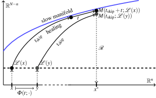
Figure 3: Visualization of the implicit scheme (5). The macroscopic time stepper $\Phi$ maps the macroscopic state $x$ to the yet unknown macroscopic state $y$. The scheme lift-evolve-restrict is applied to both states. Additionally to the healing step $t_{\mathrm{skip}}$ the dynamics on the slow manifold are observed for state $x$ for an additional (long) time $t$. Both “paths” are compared at the macroscopic end point $x^{*}$. Note, that this scheme defines $y$ implicitly.

required functions: lift, evolve, restrict (cf. main text)

solution at time t0: x function res = Phi(t,x) u1 = lift(x); u2 = evolve(t,u1); res = restrict(u2); end

explicit scheme	implicit scheme
y = Phi(t,x);	choose dy, tol, y[0] = x, n = 0, err = 2*tol function res = F(y) res = Phi(tskip,y) - Phi(tskip+t,x); end while err > tol Fy = F(y[n]); dF = Jacobian(F,y[n],dy); y[n+1] = y[n] - (dF)^(-1)*(Fy); err = abs(y[n+1] - y[n]); n = n+1; end y = y[n];

Table 1: Pseudocode algorithm for computing the macroscopic solution $y$ after time $t$ using the macroscopic time stepper for the solution $x$ using the explicit (6) and implicit (5) scheme, respectively. The implicit scheme uses a Newton iteration with a given tolerance tol to find $y$. For one-dimensional $y$ the Jacobian dF is given by (F(y[n]+dy)-F(y[n]))/dy. Note, that the complexity of the implicit scheme stems mainly from the Newton iteration, which is not specific for equation-free computations.

Advantages of equation-free methods

What additional benefits can the macroscopic time stepper $\Phi$ have beyond simulation of the low-dimensional dynamics (which could have been accomplished by running long-time simulations using $M$ directly)?

• Finding locations of macroscopic equilibria regardless of their dynamical stability: macroscopic equilibria $x$ are given by solutions to the $n$-dimensional implicit equation $\Phi(t_{0};x)=x$, or, in terms of lifting and restriction:

  $$\mathcal{R}M(t_{\mathrm{skip}}+t_{0};\mathcal{L}x)=\mathcal{R}M(t_{\mathrm{skip}};\mathcal{L}x)$$ (8)

  for a suitably chosen time $t_{0}$ (a good choice is of the same order of magnitude as $t_{\mathrm{skip}}$). The stability of an equilibrium $x$, found by solving (8), is determined by solving the generalized eigenvalue problem $Ax=\lambda Bx$ with the Jacobian matrices

  $$A=\frac{\partial}{\partial x}\mathcal{R}M(t_{\mathrm{skip}}+t_{0};\mathcal{L}x)\mbox{,\quad}B=\frac{\partial}{\partial x}\mathcal{R}M(t_{\mathrm{skip}};\mathcal{L}x)\mbox{.}$$

  Stability is determined by the modulus of the eigenvalues $\lambda$ (where $|\lambda|<1$ corresponds to stability).

• Projective integration of (7): one can integrate the macroscopic system (7) by point-wise approximation of the right-hand side $F$ and a standard numerical integrator. For example, the explicit Euler scheme for (7) would determine the value $x_{k+1}\approx x((k+1)\Delta t)$ from $x_{k}\approx x(k\Delta t)$ implicitly by approximating

  $$F(x_{k})=\frac{1}{\delta}\left[\mathcal{R}M(t_{\mathrm{skip}}+\delta;\mathcal{L}x_{k})-\mathcal{R}M(t_{\mathrm{skip}};\mathcal{L}x_{k})\right]$$

  with a small time $\delta$, and then solving the implicit equation

  $$\mathcal{R}M(t_{\mathrm{skip}};\mathcal{L}x_{k+1})-\mathcal{R}M(t_{\mathrm{skip}};\mathcal{L}x_{k})=F(x_{k})$$

  with respect to $x_{k+1}$. Projective integration is useful if the macroscopic time step $\Delta t$ can be chosen such that $\Delta t\gg\delta$, or for negative $\Delta t$, enabling integration backward in time for the macroscopic system (7).

• Matching the restriction: Sometimes it is useful to find a “realistic” microscopic state $u$, corresponding to a given macroscopic value $x$. “Realistic” corresponds in this context to “after rapid transients have settled”. This can be accomplished by solving the nonlinear equation

  $$\mathcal{R}M(t_{\mathrm{skip}};\mathcal{L}y)=x$$ (9)

  for $y$ and then setting $u=M(t_{\mathrm{skip}};\mathcal{L}y)$.

The formulas (8) and (9) have already been presented and tested in Vandekerckhove2011 , where they were found to have vastly superior performance compared to alternative proposals for consistent lifting (such as presented in Gear2005 ; Zagaris2009 ; Zagaris2012 ).

Bifurcation analysis and numerical continuation

Building on top of the basic uses of the macroscopic time stepper $\Phi$, one can also use advanced tools for the study of parameter-dependent systems. Suppose that the microscopic time stepper $M$ (and, thus, the macroscopic time stepper $\Phi$) depends on a system parameter $p$. We are interested in how macroscopic equilibria and their stability change as we vary $p$. In the examples in Sections 3 and 4 the primary system parameter is the target velocity (traffic) and door width (pedestrians), respectively.

Figure 4: Pseudo-arclength continuation of a curve of fixed points $\{(p,x):\Phi(t_{0};x,p)=x\}$ of the macroscopic time stepper $\Phi$. A new point $(\bar{p},\bar{x})$ is computed along the secant through $(p_{\ell-2},x_{\ell-2})$ and $(p_{\ell-1},x_{\ell-1})$ in a so-called predictor step. The following corrector step solves the equilibrium condition (cf. (10)) in the perpendicular direction to find the next equilibrium $(p_{\ell},x_{\ell})$ on the curve.

When tracking equilibria in a parameter-dependent problem one may start at a parameter value $p_{0}$, where the desired equilibrium $x_{0}$ (given by $\Phi(t_{0};x_{0},p_{0})=x_{0}$) is stable so that it can be found by direct simulations. This achieves a good initial guess, which is required to solve the nonlinear equations (8) reliably with a Newton iteration for near-by $p$ close to $p_{0}$. In the traffic system studied in Section 3 the equilibrium corresponding to a single phantom jam undergoes a saddle-node bifurcation (also called fold, that is, the equilibrium turns back in the parameter changing its stability, see Fig. 5(a) for an illustration). In order to track equilibria near folds one needs to extend the nonlinear equation for the macroscopic equilibrium with a so-called pseudo-arclength condition, and solve for the equilibrium $x$ and the parameter $p$ simultaneously Beyn2002 ; Kuznetsov2004 . That is, suppose we have already found a sequence $(p_{k},x_{k})$, $k=1,\ldots,\ell-1$, of equilibria and parameter values. We then determine the next pair $(p_{\ell},x_{\ell})$ by solving the extended system for $(p_{\ell},x_{\ell})$:

$$0 =\Phi(t_{0};x_{\ell},p_{\ell})-x_{\ell}\quad$$ equilibrium condition (10)

$$s =\bar{p}_{\ell}(p_{\ell}-p_{\ell-1})+\bar{x}^{T}_{\ell}(x_{\ell}-x_{\ell-1})\quad$$ pseudo-arclength condition.

The vector

$$(\bar{p}_{\ell},\bar{x}^{T}_{\ell})=\frac{(p_{\ell-1}-p_{\ell-2},x^{T}_{\ell-1}-x^{T}_{\ell-2})}{|(p_{\ell-1}-p_{\ell-2},x^{T}_{\ell-1}-x^{T}_{\ell-2})|}$$ (11)

is the secant through the previous two points, scaled to unit length, and $s$ is the approximate desired distance of the newly found point $(p_{\ell},x_{\ell})$ from its predecessor $(p_{\ell-1},x_{\ell-1})$. The continuation method (10) permits one to track equilibria through folds such as shown in Fig. 5(a) or Hopf bifurcations such as shown in Fig. 6(b) (where the equilibrium becomes unstable and small-amplitude oscillations emerge). For a more detailed review on methods for bifurcation analysis the reader is referred to standard references, e.g., Beyn2002 ; Kuznetsov2004 .

3 Traffic Models

We apply the methods introduced in Section 2 to the optimal velocity (OV) model Bando1995 as an example of microscopic traffic models. The model captures the main features of experiments of cars on a ring road Sugiyama2008 . We exploit equation-free numerical bifurcation analysis to answer the following questions; 1) for which parameter values in the OV model do we expect traffic jams and 2) how severe are they?

The equations of motion for car $n$ in the OV model are

$$\tau\ddot{x}_{n}+\dot{x}_{n}=V(x_{n+1}-x_{n}),\qquad V(\Delta x_{n})=v_{0}(\tanh(\Delta x_{n}-h)+\tanh(h)),$$ (12)

where $\tau=0.588$ is the reaction time and $V$ is the optimal velocity function depending on the velocity parameter $v_{0}$ and inflection point $h$. Periodic boundary conditions $x_{n+N}=x_{n}+L$ are used for $N=60$ cars on a ring road of length $L=60$. Depending on the choice of $v_{0}$ and $h$ one observes uniform flow, i.e., all cars have headway $\Delta x_{n}=1$, or a traffic jam, i.e., a region of high density of cars. It is worth noting, that bistable parameter regimes can exist, i.e., a stable uniform flow and a stable traffic jam coexist and one or the other emerges, depending on initial conditions.

First, we fix $h=1.2$ and study the bifurcation diagram in dependence of $v_{0}$. Before we are able to apply the algorithms presented in Section 2, we have to define the lifting and restriction operators.

The restriction and lifting operators

The restriction operator $\mathcal{R}$, used to compute the macroscopic variable to describe phenomena of interest (here the deviation of the density profile from a uniform flow) of the microscopic model on a coarse level, is chosen as the standard deviation of the distribution of headway values

$$\mathcal{R}(u)=\sigma=\sqrt{\frac{1}{N-1}\sum_{n=1}^{N}\left(\Delta x_{n}-\langle\Delta x\rangle\right)^{2}},$$ (13)

where $\langle\Delta x\rangle$ is the mean headway.

As the numerical continuation operates in a local neighborhood of the states, the lifting operator can be based on a previously computed microscopic reference state $\tilde{u}=(\tilde{x},\tilde{y})$ for positions $\tilde{x}$ and velocities $\tilde{y}$ and its macroscopic image under $\mathcal{R}$, $\tilde{\sigma}=\mathcal{R}\tilde{u}$. We use $\tilde{u}$ and $\tilde{\sigma}$ to obtain a microscopic profile $u$ for every $\sigma\approx\tilde{\sigma}$:

$$\mathcal{L}_{\mu}(\tilde{u},\sigma)=u=(x,y)=\left(x_{\text{new}},V(x_{\text{new}})\right),\quad x_{\text{new}}=\frac{\mu\sigma}{\tilde{\sigma}}(\Delta\tilde{x}-\langle\Delta\tilde{x}\rangle)+\langle\Delta\tilde{x}\rangle\mbox{.}$$ (14)

We let the lifting $\mathcal{L}_{\mu}$ depend on an artificial parameter $\mu$. We will vary $\mu$ later to demonstrate that the resulting bifurcation diagram is independent of the particular choice of $\mathcal{L}$.

Numerical results

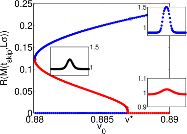
(a) Bifurcation diagram, $h=1.2$

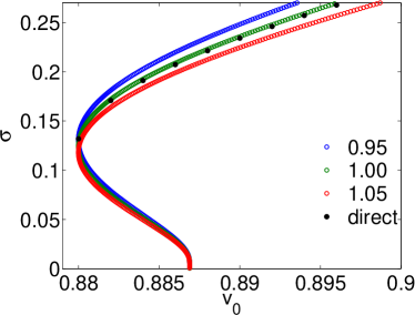
(b) Unhealed bifurcation diagrams
$\mu=0.95,1.00,1.05$

(c) Two-parameter continuation

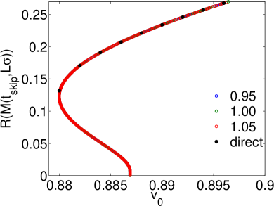
(d) Healed bifurcation diagrams
$\mu=0.95,1.00,1.05$

Figure 5: Equation-free bifurcation analysis for the optimal velocity model (12). (a) Bifurcation diagram in healed quantities for $h=1.2$. Headway profiles are shown for selected points (black circles) along the branch. Blue and red dots denote stable and unstable solutions, respectively. (b) and (d) show bifurcation diagrams for different lifting operators. Healed values in (d) lie exactly on the same branch and recover the results from direct simulation (black dots). Thus, the choice of lifting operator $\mathcal{L}$ does not affect the results if one reports the healed values (in contrast to (b), reporting the solutions $\sigma$ of (8)). (c) Two-parameter bifurcation diagram for continuation of the fold point. Saddle-node (blue crosses) and Hopf points (green dots) from measurements in one-dimensional diagrams are in perfect agreement with the continuation in two parameters $h$ and $v_{0}$ and the analytical curve (black line).

The results of the equation-free bifurcation analysis are shown in Fig. 5. The bifurcation diagram for fixed $h=1.2$ (cf. Fig. 5(a)) shows a stable traffic jam for parameter values $v_{0}>v^{*}=0.887$. By continuation of the solution from a stable traffic jam towards smaller values of $v_{0}$ a saddle-node bifurcation is found at $v_{0}=0.88$. The traffic jam loses stability and an unstable solution exists for $v_{0}\in[0.88,0.887]$. Continuing further along the branch, a Hopf bifurcation, i.e., a macroscopic pitchfork bifurcation, where traffic jams are born as small-amplitude time-periodic patterns, is found at $v_{0}=0.887$. At this point, stable uniform flow solutions ($\sigma=0$) change their stability to unstable uniform flow solutions. For $v_{0}\in[0.88,0.887]$ two stable solutions coexist. In this one-dimensional system, the unstable solution separates the stable and the unstable fixed point, acting as a barrier. Thus, the bifurcation diagram also informs us about the magnitude of the disturbance necessary to change the behavior of the system from a stable traffic jam to a stable free flow. Headway profiles are shown for selected points along the branch to illustrate the microscopic solutions. In Fig. 5(b) and Fig. 5(d) the comparison of different lifting operators is shown. While the unhealed values $\sigma$ (cf. Fig. 5(b)) of the equilibrium depends on the choice of $\mu$, the healed values $\mathcal{R}M(t_{\mathrm{skip}};\mathcal{L}\sigma)$, used in the implicit equation-free methods (cf. Fig. 5(d) and Marschler2013 ) are in perfect agreement with results from direct simulations (black dots).

In order to study the dependence on both parameters $v_{0}$ and $h$ simultaneously, we use an extended set of equations to continue the saddle-node bifurcation point in Fig. 5(c). Blue crosses and green dots denote measurements of the saddle-node and Hopf points from one-parameter continuations, respectively. The two-parameters continuation (red dots) is in perfect agreement with the measurements. As a check of validity, the Hopf curve (black line below red dots) can be computed analytically (cf. e.g., Marschler2013 ) and is shown for comparison.

In conclusion, the analysis pinpoints the parameter values for the onset and collapse of traffic jams. This information is of potential use to understand the role of speed limits. The two-parameter bifurcation diagram in Fig. 5(c) shows a free flow regime for small $v_{0}$ and large $h$ (bottom right part of the diagram). On the other hand, a large velocity parameter $v_{0}$ and a small safety distance $h$ lead to traffic jams (top left part). In between, a coexistence between free flow and traffic jams is found. The final state depends on the initial condition. A speed limit lower than the saddle-node values is necessary to assure a global convergence to the uniform free flow.

4 Pedestrian Models

For further demonstration of the equation-free bifurcation analysis, we also apply it to a social force model describing pedestrian flow Helbing1995 ; Seyfried2006 . A particular setup with two crowds passing a corridor with bottleneck Zhang2012 from opposite sites (the crowd marked blue moving to the right, the crowd marked red moving to the left) is analyzed with respect to qualitative changes of the system behavior Corradi2012 ; MarschlerStarkeLiuKevrekidis14 . To this end, a coarse bifurcation analysis is used to determine which bifurcations occur and thereby to understand which solutions are expected to exist. Details about the model and the analysis of the bottleneck problem can be found in Corradi2012 . Here, we focus on the coarse analysis of the problem.

Two parameters have been chosen as the main bifurcations parameters; the ratio of desired velocities of the two crowds $r_{v_{0}}=v_{0}^{r}/v_{0}^{b}$ and the width of the door $w$ acting as a bottleneck. Microscopic simulations of the model for two crowds of size $N=100$ reveal two fundamentally different regimes of the dynamics. One finds a blocked state and a state that is oscillating at the macroscopic level (cf. Fig. 6(a)) for small and large door widths, respectively. The question we would like to answer is: how and where does the transition from a blocked to an oscillating state happen? In mathematical terms the question is, where is the bifurcation point and what type of bifurcation is observed at the transition?

The restriction and lifting operators

We define the macroscopic quantity $m$ as

$$m=\frac{m_{r}+m_{b}}{2},\qquad m_{(r,b)}=\frac{\sum_{i\in(r,b)}\kappa(x_{i})x_{i}}{\sum_{i\in(r,b)}\kappa(x_{i})},$$ (15)

where $m_{(r,b)}$ is a weighted average of the longitudinal component for the blue and red pedestrian crowd, respectively. $\kappa$ gives more weight to pedestrians close to the door (see Corradi2012 for details). Since we expect oscillations from microscopic observations the pair of variables $(m,\dot{m})$ is used as the macroscopic variable for the equation-free methods. The transient from the initial condition to a limit cycle in the macroscopic description is shown for $w=0.7$ in Fig. 6(c). The restriction operator $\mathcal{R}=(m,\dot{m})$ is therefore defined by the macroscopic description (15) and its derivative.

The lifting operator $\mathcal{L}$ uses information about the distribution of the pedestrians in front of the door to initialize a sensible microscopic state. The distribution of positions of pedestrians along the corridor is known from numerical studies and is observed to be well-approximated by a linear density distribution, i.e., the distribution is of the form $p(|x|)=a|x|+b$, where $|x|$ is the distance from the door along the corridor axis. The slope $a$ and interception $b$ are determined by simulations for all parameter values of interest. The lifting uses these distributions to map, i.e., lift $(m,\dot{m})$ to a “physically correct” microscopic state. All velocities are initially set to $0$, such that we lift to a microscopic state with $\dot{m}=0$ (see Corradi2012 for details).

Numerical results

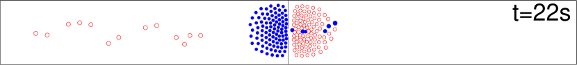
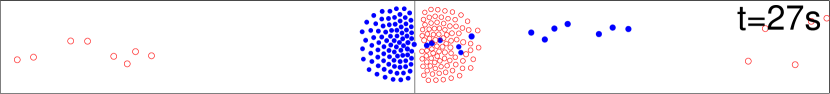
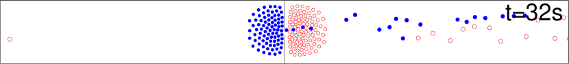
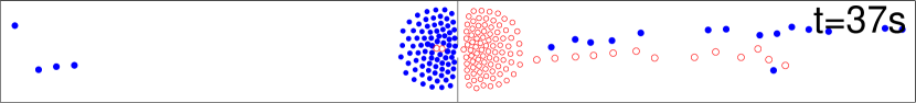
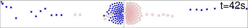
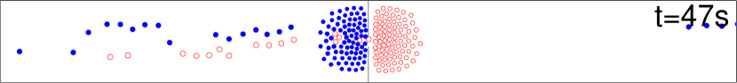
(a) Snapshots

(b) Two-parameter space

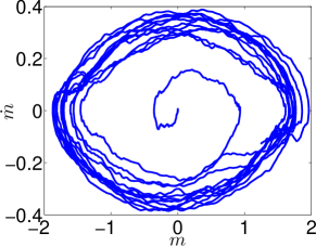
(c) Transient and limit cycle

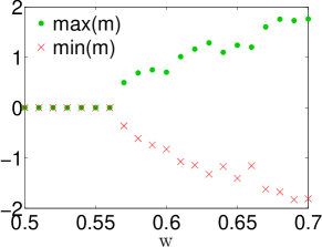
(d) Bifurcation diagram

Figure 6: Coarse analysis of the pedestrian dynamics in a corridor with bottleneck. (a) Snapshots of a microscopic simulation show oscillating behavior for large enough door width $w=0.6$. (b) Two-parameter plane explains the dynamics of the system and the point for the Hopf bifurcation. (c) Transient and limit cycle in the macroscopic description for $w=0.7$. (d) The coarse bifurcation diagram reveals a Hopf bifurcation at a critical door width $w=0.56$.

Using equation-free bifurcation analysis, the bifurcation diagram is computed for the fixed ratio $r_{v_{0}}=1$. Fig. 6(d) shows the maximum and minimum of $m(t)$ as a function of $w$. The transition from a blocked state to an oscillating state is clearly observed and the bifurcation point is found to be at $w=0.56$. The transition is analyzed in detail in Corradi2012 and the bifurcation point is identified as a Hopf bifurcation point using Poincaré sections, i.e., a discretization of the recurrent dynamics in time. This method is also implicit with a healing time $t_{\mathrm{skip}}$ determined by the first crossing of the Poincaré section. The Hopf bifurcation gives rise to macroscopic oscillations for large door width $w$ emerging from a stable blocked state for $w$ small enough.

Let us now study the influence of $r_{v_{0}}$ on the location of the bifurcation point. The system for macroscopic continuation is analyzed by a predictor-corrector method using a linear prediction and a subspace search for the correction in order to study the two-parameter problem and to continue the Hopf point. The results are shown in Fig. 6(b). Keeping the other model parameters fixed, this gives an overview of the behavior of the system on a macroscopic level in two parameters.

The application of equation-free analysis is not limited to pedestrians in a bottleneck scenario. One could also think of applications in evacuation scenarios (see, e.g., Helbing2002 ; Wagoum2012 ), where parameter regimes with blocked states have to be avoided at all cost. It is also possible to apply equation-free analysis to discrete models, e.g., cellular automaton models Burstedde2001 ; Nowak2012 . This motivates further studies using equation-free methods in traffic and pedestrian flow in order to systematically investigate and finally optimize the parameter dependencies of the macroscopic behavior of such microscopic models.

5 Discussion and Conclusion

We have demonstrated, that equation-free methods can be useful to analyze the parameter dependent behavior in traffic and pedestrian problems. Implicit methods allow us to improve the results further by reducing the lifting error. The comparison between traffic and pedestrian dynamics shows that both problem classes can be studied with the same mathematical tools. In particular, the use of coarse bifurcation analysis reveals some information about the system that could not be obtained by simpler means, e.g., direct simulations of a microscopic model, since they cannot investigate unstable solutions. Nevertheless, unstable solutions are important in order to understand the phase space and parameter dependence of the dynamics. In particular, in the case of a one-dimensional macroscopic dynamics the unstable solutions act as barriers between separate stable regimes defining reliable operating ranges. The knowledge of their locations can be used to systematically push the system over the barrier to switch to another more desirable solution, e.g., leading to a transition from traffic jams to uniform flow. In the application to two-dimensional macroscopic dynamics, we find the precise dividing line between oscillations and blocking in two parameters.

Finally, let us constrast equation-free analysis to the most obvious alternative. A common approach to determining the precise parameter value at which the onset of oscillations occurs, is to run the simulation for sufficiently long time and observe if the transient behavior vanishes. This approach suffers from two problems. First, close to the loss of linear stability in the equilibrium (i.e. close to the bifurcation point) the rate of approach to the stable orbit or fixed point is close to zero as the Jacobi matrix becomes singular. This makes the transients extremely long, resulting in unreliable numerics. Second, even eventually decaying transients may grow intermittently (the effect of non-normality) such that the criteria for the choice of the transient time to observe are non-trivial. Equation-free computations working on the macroscopic level in a neighborhood of the slow manifold do not suffer from these long transients, as they are based on direct root-finding methods.

In conclusion coarse bifurcation analysis can be used in future research to improve safety in traffic problems and evacuation scenarios of large buildings in case of emergency. The main advantage is, that realistic models can be used and a qualitative analysis of the macroscopic behavior is still possible. The method works almost independent of the underlying microscopic model and has a significant potential for helping traffic modellers to gain insight into previously inaccessible scenarios.

Acknowledgements The authors thank their collaborators R. Berkemer, A. Kawamoto and O. Corradi. The research of J. Sieber is supported by EPSRC grant EP/J010820/1. J. Starke was partially funded by the Danish Research Council under 09-065890/FTP and the Villum Fonden (VKR-Centre of Excellence “Ocean Life”).

References

- (1) D. Helbing, P. Molnár, Phys. Rev. E 51, 4282 (1995)
- (2) D. Helbing, Rev. Mod. Phys. 73, 1067 (2001)
- (3) O. Corradi, P. Hjorth, J. Starke, SIAM Journal on Applied Dynamical Systems 11(3), 1007 (2012)
- (4) M. Bando, K. Hasebe, A. Nakayama, A. Shibata, Y. Sugiyama, Phys. Rev. E 51(2), 1035 (1995)
- (5) I. Gasser, G. Sirito, B. Werner, Physica D: Nonlinear Phenomena 197, 222 (2004)
- (6) Y. Sugiyama, M. Fukui, M. Kikuchi, K. Hasebe, A. Nakayama, K. Nishinari, S.i. Tadaki, S. Yukawa, New J. Phys. 10(3) (2008)
- (7) G. Orosz, B. Krauskopf, R. Wilson, Physica D: Nonlinear Phenomena 211, 277 (2005)
- (8) C. Marschler, J. Sieber, R. Berkemer, A. Kawamoto, J. Starke, ArXiv e-prints (2013)
- (9) H. Haken, Synergetics. An introduction. (Springer, Berlin, 1983)
- (10) H. Haken, Advanced synergetics. (Springer, Berlin, 1983)
- (11) N. Fenichel, Journal of Differential Equations 31, 53 (1979)
- (12) I.G. Kevrekidis, C.W. Gear, J.M. Hyman, P.G. Kevrekidis, O. Runborg, C. Theodoropoulos, Communications in Mathematical Sciences 1, 715 (2003)
- (13) I.G. Kevrekidis, C.W. Gear, G. Hummer, AIChE Journal 50(7), 1346 (2004)
- (14) I.G. Kevrekidis, G. Samaey, Annual Review of Physical Chemistry 60(1), 321 (2009)
- (15) Y. Kevrekidis, G. Samaey, Scholarpedia 5(9), 4847 (2010)
- (16) J. Sieber, B. Krauskopf, Nonlinear Dynamics 51(3), 365 (2008)
- (17) E. Bureau, F. Schilder, I.F. Santos, J.J. Thomsen, J. Starke, Journal of Sound and Vibration 332(22), 5883 (2013)
- (18) D.A.W. Barton, J. Sieber, Phys. Rev. E 87, 052916 (2013)
- (19) C.W. Gear, T.J. Kaper, I.G. Kevrekidis, A. Zagaris, SIAM Journal on Applied Dynamical Systems 4, 711 (2005)
- (20) A. Zagaris, C.W. Gear, T.J. Kaper, Y.G. Kevrekidis, ESAIM: Mathematical Modelling and Numerical Analysis 43(04), 757 (2009)
- (21) A. Zagaris, C. Vandekerckhove, C.W. Gear, T.J. Kaper, I.G. Kevrekidis, Discrete and Continuous Dynamical Systems - Series A 32(8), 2759 (2012)
- (22) C. Vandekerckhove, B. Sonday, A. Makeev, D. Roose, I.G. Kevrekidis, Computers & Chemical Engineering 35(10), 1949 (2011)
- (23) W.J. Beyn, A. Champneys, E. Doedel, W. Govaerts, Y.A. Kuznetsov, B. Sandstede, in Handbook of Dynamical Systems, Handbook of Dynamical Systems, vol. 2, ed. by B. Fiedler (Elsevier Science, 2002), pp. 149 – 219
- (24) Y.A. Kuznetsov, Elements of Applied Bifurcation Theory, Applied Mathematical Sciences, vol. 112, 3rd edn. (Springer, New York, 2004)
- (25) A. Seyfried, B. Steffen, T. Lippert, Physica A: Statistical Mechanics and its Applications 368(1), 232 (2006)
- (26) J. Zhang, W. Klingsch, A. Schadschneider, A. Seyfried, Journal of Statistical Mechanics: Theory and Experiment 2012(02), P02002 (2012)
- (27) C. Marschler, J. Starke, P. Liu, I.G. Kevrekidis, Phys. Rev. E 89, 013304 (2014)
- (28) D. Helbing, I.J. Farkas, P. Molnar, T. Vicsek, Pedestrian and evacuation dynamics 21, 21 (2002)
- (29) A.U.K. Wagoum, M. Chraibi, J. Mehlich, A. Seyfried, A. Schadschneider, Computer Animation and Virtual Worlds 23(1), 3 (2012)
- (30) C. Burstedde, K. Klauck, A. Schadschneider, J. Zittartz, Physica A: Statistical Mechanics and its Applications 295(3–4), 507 (2001)
- (31) S. Nowak, A. Schadschneider, Phys. Rev. E 85, 066128 (2012)