A Many-core Machine Model for Designing Algorithms with Minimum Parallelism Overheads

Abstract

We present a model of multithreaded computation, combining fork-join and single-instruction-multiple-data parallelisms, with an emphasis on estimating parallelism overheads of programs written for modern many-core architectures. We establish a Graham-Brent theorem for this model so as to estimate execution time of programs running on a given number of streaming multiprocessors. We evaluate the benefits of our model with four fundamental algorithms from scientific computing. In each case, our model is used to minimize parallelism overheads by determining an appropriate value range for a given program parameter; moreover experimentation confirms the model’s prediction.

1 Introduction

Designing efficient algorithms targeting implementation on hardware acceleration technologies (multi-core processors, graphics processing units (GPUs), field-programmable gate arrays) creates major challenges for computer scientists. A first difficulty is to define models of computations retaining the computer hardware characteristics that have a dominant impact on program performance. Therefore, in addition to specify the appropriate complexity measures for the algorithms to be analyzed, those models must consider the relevant parameters characterizing the abstract machine executing those algorithms. A second difficulty is, for a given model of computations, to combine its complexity measures so as to determine the “best” algorithm among different algorithmic solutions to a given problem.

In the fork-join concurrency model [1] two complexity measures, the work $T_{1}$ and the span $T_{\infty}$, and one machine parameter, the number P of processors, can be combined in results like the Graham-Brent theorem [1, 7] or the Blumofe-Leiserson theorem (Theorems 13 & 14 in [2]) in order to compare algorithm running time estimates. We recall that the Graham-Brent theorem states that the running time $T_{\mbox{\sf P}}$ on P processors satisfies $T_{\mbox{\sf P}}\leq T_{1}/{\mbox{\sf P}}+T_{\infty}$. A refinement of this theorem supports the implementation (on multi-core architectures) of the parallel performance analyzer Cilkview [10]. In this context, the running time $T_{\mbox{\sf P}}$ is bounded in expectation by $T_{1}/{\mbox{\sf P}}+2{\delta}\widehat{T_{\infty}}$, where ${\delta}$ is a constant (called the span coefficient) and $\widehat{T_{\infty}}$ is the burdened span.

With the pervasive ubiquity of many-core processors, in particular GPUs, it is desirable for models of computations to combine explicitly both task-based parallelism and data-based parallelism. In fact, popular concurrency platforms (CilkPlus [11, 18], CUDA [16, 17] and OpenCL [22]) offer both forms of parallelism, with language constructs specific to each case. Meanwhile, classical models of parallel computations, like the fork-join concurrency model or the PRAM model [21, 5], do not distinguish between task-based and data-based parallelism, which is too simplistic for analyzing algorithms targeting the above concurrency platforms. In addition, the PRAM model fails to retain important features of actual computers related to memory traffic, such as cache complexity [4].

An attempt to integrate memory contention into the PRAM model has been made with the QRQW (Queue Read Queue Write) PRAM, defined in [6] by Gibbons, Matias and Ramachandran. The authors also enhance the Graham-Brent theorem. However, they conflate in a single quantity time spent in arithmetic operations and time spent in read/write accesses. We believe that this unification is not appropriate for recent many-core processors, such as GPUs, for which the ratio between one global memory read/write access and one floating point operation can be in the 100’s.

In a recent paper, Ma, Agrawal and Chamberlain [13] introduce the TMM (Threaded Many-core Memory) model which retains many important characteristics of GPU-type architectures, including several machine parameters such as throughput and coalesced granularity. Moreover, TMM analysis can rank algorithms from slow to fast, given those machine parameters, while their running time estimate on P cores is not based on the Graham-Brent theorem.

Many works, such as [14, 12], targeting code optimization and performance prediction of GPU programs are related to our work. However, these papers do not define an abstract model in support of the analysis of algorithms.

In this paper, we propose a many-core machine model (MMM) which aims at minimizing parallelism overheads of algorithms targeting implementation on GPUs. In the design of this model, we insist on the following features:

• Two-level DAG programs. Defined in Section 2, this aspect captures the two levels of parallelism (fork-join and SIMD) of heterogeneous programs (like a CilkPlus program using #pragma simd [18] or a CUDA program with the so-called dynamic parallelism [17]).

• Parallelism overhead. We introduce this complexity measure in Section 2.3 with the objective of analyzing communication and synchronization costs.

• A Graham-Brent theorem. We combine three complexity measures (work, span and parallelism overhead) and two machine parameters (size of local memory and data transfer throughput) in order to estimate the running time of an MMM program on $P$ streaming multiprocessors. This result is Theorem 1 in Section 2.4.

Our proposed model extends both the fork-join concurrency model and PRAM-based models, with an emphasis on parallelism overheads resulting from communication and synchronization costs.

We sketch below how, in practice, we use this model in order to minimize parallelism overheads of programs targeting GPUs. Consider an MMM program ${\cal P}$, that is, an algorithm expressed in the MMM model. Assume that a program parameter $s$ (like the number of threads per thread-block or the amount of data transfer per thread-block) can be arbitrarily chosen within some range ${\cal S}$ while preserving the specifications of ${\cal P}$. Let $s_{0}$ be a particular value of $s$ which corresponds to an instance ${\cal P}_{0}$ of ${\cal P}$ that, in practice, can be seen as a naive (or simply initial) version of the algorithm.

Assume that, when $s$ varies within ${\cal S}$, the work, say $W_{\cal P}(s)$, does not vary much, that is, $W_{\cal P}(s_{0})/W_{\cal P}(s)$ $\in\Theta(1)$ hold. Assume also that the parallelism overhead $O_{\cal P}(s)$ varies more substantially, say $O_{\cal P}(s_{0})/O_{\cal P}(s)\in{\Theta}(s-s_{0})$. Then, we determine a value $s_{\rm min}\in{\cal S}$ maximizing the ratio $O_{\cal P}(s_{0})/O_{\cal P}(s)$. Next, we use our version of Graham-Brent theorem (more precisely, we use Corollary 1) to check that the upper bound for the running time of ${\cal P}(s_{\rm min})$ is less than that of ${\cal P}(s_{o})$. If this holds, we view ${\cal P}(s_{\rm min})$ as a solution of our problem of algorithm optimization (in terms of parallelism overheads).

To demonstrate and evaluate the benefits of our model, and the above optimization strategy, we applied them successfully to four fundamental algorithms in scientific computing, see Sections 3 to 6. These four applications are the univariate polynomial division and multiplication, radix sort and the Euclidean algorithm. Each of them satisfies the hypotheses of the above optimization strategy. Our theoretical analysis, for three of these applications, has led to an optimized implementation reported in [9] and publicly available. while, for the other application, this analysis has explained a posteriori the experimental observations of [19].

2 A many-core machine model

The model of parallel computations presented in this paper aims at capturing communication and synchronization overheads of programs written for modern many-core architectures. One of our objectives is to optimize algorithms by techniques like reducing redundant memory accesses. The reason for this optimization is the fact that, on actual GPUs, global memory latency is approximately 400 to 800 clock cycles, while local memory latency is only a few clock cycles. This memory latency difference, when not properly taken into account, may have a dramatically negative impact on program performance. As mentioned in the introduction, this hardware feature of GPUs cannot be captured by the well-studied PRAM model. Indeed, any memory access, as well as any integer arithmetic operation, is performed in unit time on a PRAM machine.

This latter, as well as other limitations, have motivated variants of the PRAM model, including our work. Another motivation, mentioned above, is the fact that popular concurrency platforms offer task-based and data-based parallelisms, with language constructs specific to each case.

As specified in Sections 2.1 and 2.2, our many-core machine model (MMM) retains many of the characteristics of modern GPU architectures programming models like CUDA or OpenCL. However, in order to support algorithm analysis with an emphasis on parallelism overheads, as defined in Section 2.3 and 2.4, MMM abstract machines admit a few simplifications and limitations with respect to actual many-core devices.

2.1 Characteristics of the abstract many-core machines

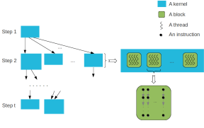
Figure 1: Overview of a many-core machine program

Architecture. An MMM abstract machine possesses an unbounded number of streaming multiprocessors (SMs) which are all identical. Each SM has a finite number of processing cores and a fixed-size local memory. An MMM machine has a two-level memory hierarchy, comprising an unbounded global memory with high latency and low throughput while SMs local memories have low latency and high throughput.

Programs. An MMM program is a directed acyclic graph (DAG) whose vertices are kernels (defined hereafter) and edges indicate serial dependencies, similarly to the instruction stream DAGs of the fork-join multithreaded concurrency model. A kernel is an SIMD (single instruction, multiple data) program capable of branches and decomposed into a number of thread-blocks. Each thread-block is executed by a single SM and each SM executes a single thread-block at a time. Similarly to a CUDA program, an MMM program specifies for each kernel the number of thread-blocks and the number of threads per thread-block, following the same extended function-call syntax. Figure 1 depicts the different types of components of an MMM program.

Scheduling and synchronization. At run time, an MMM machine schedules thread-blocks (from the same or different kernels) onto SMs, based on the dependencies specified by the edges of the DAG and the hardware resources required by each thread-block. Threads within a thread-block can cooperate with each other via the local memory of the SM running the thread-block. Meanwhile, thread-blocks interact with each other via the global memory. In addition, threads within a thread-block are executed physically in parallel by an SM. Moreover, the programmer cannot make any assumptions on the order in which thread-blocks of a given kernel are mapped to the SMs. Hence, MMM programs run correctly on any fixed number of SMs.

Memory access policy. All threads of a given thread-block can access simultaneously any memory cell of the local memory or the global memory: read/write conflicts are handled by the CREW (concurrent read, exclusive write) policy. However, read/write requests to the global memory by two different thread-blocks cannot be executed simultaneously. In case of simultaneous requests, one thread-block is chosen randomly and served first, then the other is served.

For the purpose of analyzing program performance, we define two machine parameters:

• Time (expressed in clock cycles) to transfer one machine word between the global memory and the local memory of any SM.

• Size (expressed in machine words) of the local memory of any SM.

Thus, the quantity $1/U$ is a throughput measure and has the following property. If $\alpha$ and $\beta$ are the numbers of words respectively read and written to the global memory by one thread of a thread-block $B$, then the total time $T_{D}$ spent in data transfer between the global memory and the local memory of an SM executing $B$ satisfies

$$T_{D}\ \leq\ (\alpha+\beta)U.$$ (1)

We observe that, on actual machines, some hardware characteristics may reduce data transfer time (like coalesced accesses to global memory) or the contribution of the latter on the overall running time (like concurrent execution of thread-blocks on the same SM with fast context switching in order to hide data transfer latency). Other hardware characteristics (like partition camping) may increase data transfer time. However, this reduced or increased transfer time will remain in $O(\alpha+\beta)$. Therefore, the fact that MMM machines do not have these hardware characteristics will not lead us to incorrect asymptotic upper bounds when estimating the running time of MMM programs.

Similarly, the local memory size $Z$ unifies different characteristics of an SM and, thus, of a thread-block. Indeed, each of the following quantities is at most equal to $Z$: the number of cores of an SM, the number of threads of a thread-block, the number of words in a data transfer between the global memory and the local memory of an SM.

Relation (1) calls for another comment. One could expect the introduction of a third machine parameter, say $V$, which would be the time to execute one local operation (arithmetic operation, read/write in the local memory), such that, if $\sigma$ is the total number of local operations performed by one thread of a thread-block $B$, then the total time $T_{A}$ spent in local operations by an SM executing $B$ would satisfy $T_{A}\ \leq\ \sigma V.$ Therefore, for the total running time $T$ of the thread-block $B$, we would have

$$T\ =\ T_{A}+T_{D}\ \leq\ \sigma V+(\alpha+\beta)U.$$ (2)

Instead of introducing this third machine parameter $V$, we let $V=1$. In other words, $U$ is the ratio between the time to transfer a machine word and the time to execute a local operation. We assume $U>1$.

Finally, Relation (2) requires another justification. Indeed, this estimate suggests that, at every clock cycle, every thread is either performing an arithmetic operation or accessing memory. For this to be true, conditional branches responsible for code divergence [8] need to be eliminated by techniques like code replication [20], such that all threads execute the same code path. However, in a sake of clarity, we will not perform this transformation in the MMM algorithms stated in the subsequent sections. In fact, we verified experimentally that the impact of code divergence on the performance of our algorithms is negligible.

2.2 Many-core machine programs

Recall that each MMM program ${\cal P}$ is a DAG $({\cal K},{\cal E})$, called the kernel DAG of ${\cal P}$, where each node $K\in{\cal K}$ represents a kernel, and each edge $E\in{\cal E}$ records the fact that a kernel call must precede another kernel call. In other words, a kernel call can be executed provided that all its predecessors in the DAG $({\cal K},{\cal E})$ have completed their execution.

Synchronization costs. Recall that each kernel decomposes into thread-blocks and that all threads within a given kernel execute the same serial program, but with possibly different input data. In addition, all threads within a thread-block are executed physically in parallel by an SM. It follows that MMM kernel code needs no synchronization statement, like CUDA’s __syncthreads(). Consequently, the only form of synchronization taking place among the threads executing a given thread-block is that implied by code divergence. This latter phenomenon can be seen as parallelism overhead. As mentioned, an MMM machine handles code divergence by eliminating the corresponding conditional branches via code replication and the corresponding cost will be captured by the complexity measures (work, span and parallelism overhead) of the MMM model. Since no synchronization occurs between thread blocks, we turn our attention to scheduling.

Scheduling costs. Since an MMM abstract machine has infinitely many SMs and since the kernel DAG defining an MMM program ${\cal P}$ is assumed to be known when ${\cal P}$ starts to execute, scheduling ${\cal P}$’s kernels onto the SMs can be done in time $O(\Gamma)$ where $\Gamma$ is the total length of ${\cal P}$’s kernel code. Thus, we shall neglect those costs in comparison to the costs of transferring data between SMs’ local memories and the global memory. We also note that assuming that, the kernel DAG is known when ${\cal P}$ starts to execute, allows us to focus on parallelism overheads resulting from this data transfer. Extending MMM machines to support programs whose instruction stream DAGs unfold dynamically at run time and integrating the resulting scheduling costs as in [10] is left for future work.

Thread block DAG. Since each kernel of the program ${\cal P}$ decomposes into a finite number of thread-blocks, we map ${\cal P}$ to a second graph, called the thread block DAG of ${\cal P}$, whose vertex set ${\cal B}({\cal P})$ consists of all thread-blocks of the kernels of ${\cal P}$ and such that $(B_{1},B_{2})$ is an edge if $B_{1}$ is a thread-block of a kernel preceding the kernel of the thread-block $B_{2}$ in ${\cal P}$. This second graph defines two important quantities:

$N({\cal P})$:

number of vertices in the thread-block DAG of ${\cal P}$,

$L({\cal P})$:

critical path length (where length of a path is the number of edges in that path) in the thread-block DAG of ${\cal P}$.

2.3 Complexity measures for the many-core machine model

Consider an MMM program ${\cal P}$ given by its kernel DAG $({\cal K},{\cal E})$. Let $K\in{\cal K}$ be any kernel of ${\cal P}$ and $B$ be any thread-block of $K$. We define the work of $B$, denoted by $W(B)$, as the total number of local operations performed by all threads of $B$. We define the span of $B$, denoted by $S(B)$, as the maximum number of local operations performed by a thread of $B$. Let $\alpha$ and $\beta$ be the maximum numbers of words read and written (from the global memory) by a thread of $B$. Then, we define the overhead of $B$, denoted by $O(B)$, as $(\alpha+\beta)\,U$. Next, the work (resp. overhead) $W(K)$ (resp. $O(K)$) of the kernel $K$ is the sum of the works (resp. overheads) of its thread-blocks, while the span $S(K)$ of the kernel $K$ is the maximum of the spans of its thread-blocks.

We consider now the entire program ${\cal P}$. The work $W({\cal P})$ of ${\cal P}$ is defined as the total work of all its kernels

$$W({\cal P})=\sum_{K\in{\cal K}}\,W(K).$$

Regarding the graph $(K,E)$ as a weighted-vertex graph where the weight of a vertex $K\in{\cal K}$ is its span $S(K)$, we define the weight $S({\gamma})$ of any path ${\gamma}$ from the first executing kernel to the last executing kernel as $S({\gamma})=\sum_{K\in{\gamma}}\,S(K).$ Then, we define the span $S({\cal P})$ of the program ${\cal P}$ as

$$S({\cal P})=\max_{{\gamma}}\,S({\gamma}).$$

Finally, we define the overhead $O({\cal P})$ of the program ${\cal P}$ as the total overhead of all its kernels

$$O({\cal P})=\sum_{K\in{\cal K}}\,O(K).$$

Observe that, according to Mirsky’s theorem [15], the number ${\pi}$ of parallel steps in ${\cal P}$ (i.e. anti-chains in $({\cal K},{\cal E})$) is equal to the maximum length of a path in $({\cal K},{\cal E})$ from the first executing kernel to the last executing kernel.

2.4 A Graham-Brent theorem with overhead

Theorem 1

We have the following estimate for the running time $T_{P}$ of the program ${\cal P}$ when executed on P SMs:

$$T_{\mbox{\sf P}}\leq(N({\cal P})/{\mbox{\sf P}}+L({\cal P}))C({\cal P})$$ (3)

where $C({\cal P})=\max_{B\in{\cal B}({\cal P})}\,(S(B)+O(B))$,

The proof is similar to that of the original result. One observes that the total number of complete steps (for which $P$ thread-blocks can be scheduled by a greedy scheduler) is at most $N({\cal P})/{\mbox{\sf P}}$ while the number of incomplete steps is at most $L({\cal P})$. Finally, $C({\cal P})$ is an obvious upper bound for the running time of every step, complete or incomplete.

The proof of the following corollary follows from Theorem 1 and from the fact that costs of scheduling thread-blocks onto SMs are neglected.

Corollary 1

Let K be the maximum number of thread blocks along an anti-chain of the thread-block DAG of ${\cal P}$. Then the running time $T_{\cal P}$ of the program ${\cal P}$ satisfies:

$$T_{\cal P}\leq(N({\cal P})/{\mbox{\sf K}}+L({\cal P}))C({\cal P})$$ (4)

Corollary 1 allows us to estimate the running time of an MMM program as a function of the machine parameters $Z$, $U$ and the thread-block DAG of ${\cal P}$. Thus this estimate does not depend on the number of SMs in use to execute ${\cal P}$.

3 Polynomial division

Our first application of the MMM deals with univariate polynomial division. One division step, like a Gaussian elimination step, performs a linear combination of two vectors. Hence, the ideas developed in this section would apply to linear algebra and are not specific to polynomial arithmetic.

Let ${\mathbb{K}}$ be a field and $a,b\in{\mathbb{K}}[X]$ be univariate polynomials with coefficients in ${\mathbb{K}}$, with $b\neq 0$. Assume that each arithmetic operation (addition, subtraction, multiplication and division) in ${\mathbb{K}}$ can be done with a single machine word operation on an MMM machine. Let $n$ and $m$ be non-negative integers such that we have ${\deg}(a)=n-1$ and ${\deg}(b)=m-1$. Thus, $n$ and $m$ are the number of terms (null or not) of $a$ and $b$, respectively. Let $q$ and $r$ be the quotient and the remainder in the Euclidean division of $a$ by $b$. Thus, $(q,r)$ is a unique couple of univariate polynomials over ${\mathbb{K}}$ such that $a=q\cdot b+r$ and ${\deg}(r)<{\deg}(b)$ both hold.

In Section 3.1, we present a multithreaded algorithm computing $(q,r)$ on an MMM machine. We call this algorithm naive since it implements the natural idea that, at each division step, each thread computes one coefficient of the next intermediate remainder. In Section 3.2, we propose a second MMM algorithm with the goal of minimizing data transfer. We analyze both algorithms with the complexity measures of Section 2.3. In Section 3.3, we compare their running time estimates given by Corollary 1.

3.1 Naive algorithm

In each kernel call, each thread computes one coefficient of an intermediate remainder polynomial by means of one multiplication and one subtraction in the coefficient field ${\mathbb{K}}$. Algorithm 1 repeatedly calls the kernel stated in Algorithm 2. The latter performs one division step in parallel. Let ${\ell}$ be the number of threads in a thread-block, we note that each kernel uses $\lceil\frac{m}{\ell}\rceil$ thread-blocks. We observe that each thread of a kernel reads/writes 3 to 5 words in the global memory without storing them in the local memory.

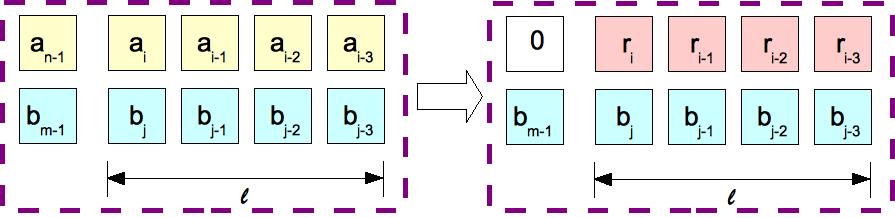
Figure 2: Naive division: illustration of a thread-block reading coefficients from $a$,$b$ and writing to $r$.

We also notice that Algorithm 1 performs exactly $n-m+1$ consecutive calls to Algorithm 2. Nevertheless, Algorithm 2 works correctly even if, after one division step, the degree of an intermediate remainder drops by more than one. This implementation choice is relevant to dense polynomials, which are our primary interest. In the sparse case, the degree of an intermediate remainder needs to be computed after each division step. Figure 2 shows a division step within a thread-block after running Algorithm 2 once.

1

Input: $a,b\in{\mathbb{K}}[X]$ with ${\deg}(a)\geq{\deg}(b)$ that is, $n-1\geq m-1$.

Output: $q,r\in{\mathbb{K}}[X]$ s. t. $a=q\cdot b+r$ and $\deg(r)<m-1$.

2 Let $\ell$ be the number of threads in a thread block;

3

4Let $q$ be array of size $n-m+1$ with coefficients in $\mathbb{K}$;

5

6for $(i=(n-1)\ldots(m-1))$ do

7       NaiveDivKernel$\lll\lceil m/{\ell}\rceil,\ell\ggg(a,b,q,i,m-1)$;

8      

9

10if $a[0]==\cdots==a[m-1]==0$ then

11       return $[q,0]$;

12      

13

14Compute $k$, the maximum $i$ such that $a[i]\neq 0$ holds;

15

16Let $r$ be array of size $k+1$ s.t. $r[i]=a[i]$ for $0\leq i\leq k$;

17

18return $[q,r]$;

19

Algorithm 1 NaivePlainDivisionGPU($a,b$)

1

Input: $a,b,q\in{\mathbb{K}}[X]$, $d_{b}=\deg(b)$, $i\in{\mathbb{N}}$, $d_{b}\leq i$.

2Let blockID, blockDim, threadID be the block id, number of threads per block, thread id respectively;

3 $j=$blockID$\cdot$blockDim $+$ threadID;

4

5if $j\leq d_{b}$ then

6      

7       if $j==0$ then

             /* writing to global memory */

8             $q[i-d_{b}]=(b[d_{b}])^{-1}\cdot a[i]$;

9            

10      

      /* updating $a$ in global memory */

11       $a[j+i-d_{b}]$ -= $b[j]\cdot(b[d_{b}])^{-1}\cdot a[i]$;

12      

Algorithm 2 NaiveDivKernel($a,b,q,i,d_{b}$)

We denote by $W_{1}$, $S_{1}$ and $O_{1}$, the work, span and overhead of Algorithm 1, respectively. Since each thread-block performs $2\,{\ell}+1$ arithmetic operations and each thread makes at most 5 accesses to the global memory, we obtain $W_{1}=\frac{(n-m+1)\,m\,(2\,{\ell}+1)}{\ell}$, $S_{1}=3\,(n-m+1)$ and $O_{1}=\frac{5\,(n-m+1)\,m\,U}{\ell}$. To apply Corollary 1, we shall compute the quantities $N({\cal P})$, $L({\cal P})$ and $C({\cal P})$ defined in Section 2. We denote them here by $N_{1}$, $L_{1}$ and $C_{1}$, respectively. One can easily check that we have $N_{1}=\frac{(n-m+1)\,m}{\ell}$, $L_{1}=n-m+1$ and $C_{1}=3+5\,U$.

3.2 Optimized algorithm

In each kernel, each thread updates a number of coefficients (instead of just one) of an intermediate remainder polynomial repeatedly during a number of division steps, thus without synchronizing data with other thread-blocks. The motivation of this new scheme is to minimize the amount of data transferred between global and local memories. Similarly to the scheme in Section 3.1, Algorithm 3 repeatedly calls Algorithm 4. Figure 3 shows $s$ division steps within a thread-block after running Algorithm 4 once. More specifically, given an integer $s\geq 1$, Algorithm 4 performs sufficiently many division steps (at most $s$) such that the output polynomial $r$ is either zero or its degree is less than that of $a$ at least by $s$. To this end, each thread-block

uses $3\,s$ threads,

loads the coefficients of $X^{d}$, $X^{d-1}$, $\ldots$, $X^{d-s+1}$ from $a$ (resp. $b$), that we call the $s$-head of $a$ (resp. $b$), where $d$ is the degree of $a$ (resp. $b$), see Lines 3-4,

loads $2\,s$ (resp. $3\,s$) consecutive coefficients of $a$ (resp. $b$), say $X^{d_{1}}$, $X^{d_{1}-1}$, $\ldots$, $X^{d_{1}-2s+1}$ ($X^{d_{2}}$, $X^{d_{2}-1}$, $\ldots$, $X^{d_{2}-3s+1}$) for some integer $d_{1}>0$ (resp. $d_{2}>0$) which depends on the thread and thread-block IDs.

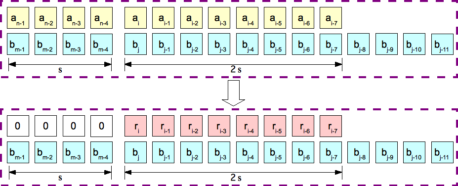
Figure 3: Optimized division: illustration of a thread-block reading coefficients from $a$,$b$ and writing to $r$.

The $s$-heads of $a$ and $b$ are used to keep track of the leading coefficient of an intermediate remainder during the entire execution of a kernel, see Lines 14-15 of Algorithm 4. This task is achieved by the first $s$ threads of a thread-block and requires $s+(s-1)+\cdots+1=\frac{s(s+1)}{2}$ arithmetic operations. Meanwhile, the other $2\,s$ threads update $2s$ coefficients of $a$, see Lines 16-17, which takes $2\,s\cdot 2\,s$ arithmetic operations. Finally, at Lines 12-13 (resp. 18-19) the quotient $q$ (resp. the intermediate remainder $a$) is updated in the global memory.

We denote the work, span and overhead of the optimized algorithm by $W_{s}$, $S_{s}$ and $O_{s}$, respectively. Since each thread makes at most 9 accesses to the global memory, we obtain $W_{s}=\frac{(n-m+1)\,m\,(9\,s+1)}{4\,s}$, $S_{s}=3\,(n-m+1)$ and $O_{s}=\frac{9\,(n-m+1)\,m\,U}{2\,s^{2}}$. To apply Corollary 1, we shall compute the quantities $N({\cal P})$, $L({\cal P})$ and $C({\cal P})$ defined in Section 2. We denote them here by $N_{s}$, $L_{s}$ and $C_{s}$, respectively. One can easily check that we have $N_{s}=\frac{(n-m+1)\,m}{2\,s^{2}}$, $L_{s}=\frac{n-m+1}{s}$ and $C_{s}=3\,s+9\,U$.

Input: $a,b\in{\mathbb{K}}[X]$ with ${\deg}(a)\geq{\deg}(b)$ that is, $n-1\geq m-1$ and $s\in{\mathbb{N}}$.

1

Output: $q,r\in{\mathbb{K}}[X]$ s. t. $a=q\cdot b+r$ and $\deg(r)<m-1$.

2

3Let $\ell=3s$ be the number of threads in a thread block;

4 Let $q$ be array of size $n-m+1$ with coefficients in $\mathbb{K}$;

5

6for $(i=n-1;i\geq m-1;i=i-s)$ do

7       OptDivKer$\lll\lceil m/(2s)\rceil,\ell\ggg(a,b,q,i,m-1,s$);

8      

9

10if $a[0]==\cdots==a[m-1]==0$ then

11       return $[q,0]$;

12      

13

14Compute $k$, the maximum $i$ such that $a[i]\neq 0$ holds;

15

16Let $r$ be array of size $k+1$ s.t. $r[i]=a[i]$ for $0\leq i\leq k$;

17

18return $[q,r]$;

Algorithm 3 OptimizePlainDivisionGPU($a,b,s$)

1

Input: $a,b,q\in{\mathbb{K}}[X]$, $i\in{\mathbb{N}}$, $d_{b}=\deg(b)$ and $s\in{\mathbb{N}}$.

2

3Let sAc, sBc, sA, sB be local arrays of size $s,s,2s,3s$ respectively each with coefficients in $\mathbb{K}$;

4

5$j=$blockID$\cdot$blockDim $+$ threadID; $t=$ threadID;

6

/* Reading from global memory */

7if $t<s$ then

8       sAc$[t]=a[i-t]$; sBc$[t]=b[d_{b}-t]$; sB$[t]=b[d_{b}-2s\,$blockID$-t]$;

9      

10

11if $t\geq s$ then

12       sA$[t-s]=a[i-s-2s\,$blockID$-t]$; sB$[t]=b[d_{b}-2s\,$blockID$-t]$;

13      

14

15for $(k=0;(k<s)\wedge(i+k\geq d);k=k+1)$ do

16       while $(k<s)\wedge($ sAc$[k]==0)$ do

17             $k=k+1$;

18            

19       if $k\geq s$ then

20             break;

21            

22      

23      if $j==0$ then

             /* Writing $q$ to global memory */

24             $q[i-d_{b}-k]$ = sAc$[k]\cdot b[d_{b}]^{-1}$;

25            

26       if $k\leq t<s$ then

27             sAc$[t]$ -= sBc$[t-k]$ $\cdot$ sAc$[k]\cdot b[d_{b}]^{-1}$;

28            

29       if $t\geq s$ then

30             sA$[t-s]$ -= sB$[t-k]$ $\cdot$ sAc$[k]\cdot b[d_{b}]^{-1}$;

31            

32      

33

34if $t\geq s$ then

       /* Writing back $a$ to global memory */

35       $a[i-s-2s\,$blockID$-t]=$ sA$[t-s]$;

36      

37

Algorithm 4 OptDivKer$(a,b,q,i,d_{b},s)$

3.3 Comparison of running time estimates

Before following the algorithm optimization strategy stated in the introduction, we replace ${\ell}$ and $s$ by $Z/2$ and $Z/7$, respectively, since $2{\ell}$ or $7s$ coefficients must fit into the local memory, that is, $2{\ell}\leq Z$ and $7s\leq Z$. Now, we observe that the work ratio $W_{1}/W_{s}$ is asymptotically constant:

$$\frac{W_{1}}{W_{s}}=\frac{8\,(Z+1)}{9\,Z+7},$$ (5)

and $S_{1}/S_{s}=1$. Then, we compute the overhead ratio:

$$\frac{O_{1}}{O_{s}}={\frac{20}{441}}\,Z.$$ (6)

We observe that this substantial improvement in data transfer overhead is done at a fairly low expense in terms of work overhead. Next, applying Corollary 1, the running time estimate of the naive and optimized algorithms are bounded over, respectively by $T_{1}=(N_{1}/{\mbox{\sf K}_{1}}+L_{1})\cdot C_{1}$ with $\mbox{\sf K}_{1}=\frac{m}{\ell}$ and $T_{s}=(N_{s}/{\mbox{\sf K}_{s}}+L_{s})\cdot C_{s}$ with $\mbox{\sf K}_{s}=\frac{m}{2\,s}$. We compute the ratio $R=T_{1}/T_{s}$, that is,

$$R=\frac{(3+5\,U)\,Z}{3\,(Z+21\,U)}.$$ (7)

We observe that $R$ is larger than $1$ if and only if $Z>12.6$ holds. The above condition clearly holds on actual GPU architectures. Thus the optimized algorithm (that is for $s>1$) is overall better than the naive one (that is for $s=1$). This is verified in practice in [9], where $s$ is set to $512$.

4 Radix sort

In [19], the authors present a CUDA implementation of the radix sort algorithm. Assuming that all entries are non-negative integers of bit-size $c$, this CUDA implementation sorts $n$ entries by performing $\frac{c}{s}$ passes where $s$ is a program parameter. In each pass, each thread-block first loads and sorts its tile using $s$ iterations of 1-bit split, and write back its $2^{s}$-entry digit histogram and sorted data. Then, it performs a prefix sum over the histogram stored in a column-major order. Finally, each thread-block copies its elements to the correct output position.

Let ${\ell}$ be the number of threads per thread-block. Following [19], we assume that each thread deals with $4$ elements. Then, for each thread-block, $4\,{\ell}$ original elements, $4\,{\ell}$ sorted elements and a $2^{s}$-entry digit histogram must fit into the local memory, hence $8\,{\ell}+2^{s}\leq Z$. Thus, the maximum overhead per thread-block is $9\,U$ (loading $4$ elements, writing back $4$ sorted elements and $1$ value of the histogram ).

We compute the work, span and overhead, respectively as $W_{s}=c\left(\frac{22\,s\,{\ell}+s+12}{4\,s\,{\ell}}+\frac{{2}^{s}+20\,{2}^{s}\,{\ell}}{16\,s\,{\ell}^{2}}+1\right)n+\frac{c\,(16+192\,{\ell})}{16\,s}$, $S_{s}=c\left(8\,\log_{2}{\ell}+\frac{16}{s}\log_{2}{\ell}+41+\frac{54}{s}\right)$, $O_{s}=c\,U\left(\frac{9}{2\,s\,{\ell}}\,n+\frac{17\,2^{s}}{16\,s\,{\ell}^{2}}\,n-\frac{1}{s}\right)$.

We view the case $s=1$ as a naive radix sort algorithm, with work, span and overhead given by $W_{1}$, $S_{1}$ and $O_{1}$, respectively. Letting $n$ escaping to infinity, the work ratio ${W_{1}}/{W_{s}}$ is asymptotically equivalent to:

$$\frac{W_{1}}{W_{s}}\ \sim\ \frac{104\,s\,{\ell}^{2}+92\,s\,{\ell}+2\,s}{88\,s\,{\ell}^{2}+16\,{\ell}^{2}+20\,2^{s}\,{\ell}+4\,s\,{\ell}+48\,{\ell}+2^{s}}.$$ (8)

Similarly, the span ratio $S_{1}/S_{s}=\frac{s\,(24\,\log_{2}{\ell}+95)}{(8\,s+16)\,log_{2}{\ell}+41\,s+54}$ is asymptotically constant, meanwhile the overhead ratio is:

$$\frac{O_{1}}{O_{s}}\ \sim\ \frac{s\,(72\,{\ell}+34)}{72\,{\ell}+17\,2^{s}}.$$ (9)

We notice that if $2^{s}=\Theta({\ell})$ holds, we can reduce the overhead by a factor of $s$ while increasing the work by a constant factor only. Meanwhile, with $2^{s}=\Theta({\ell}^{2})$, we increase both the work and the overhead by a non-constant factor. In this latter scenario, we could not optimize the naive algorithm in any sense.

To apply Corollary 1, we compute the three quantities $N_{s}=\frac{c}{s}\left({\frac{1}{2\,{\ell}}}+{\frac{{2}^{s}}{8\,{\ell}^{2}}}\right)\,n$, $L_{s}=\frac{5\,c}{s}$ and $C_{s}=s\left(41+\right.$ $\left.8\,\log_{2}{\ell}\right)+12+9\,U$. Then, the ratio $R$ of the running time estimate between the naive algorithm and that for an arbitrary $s$ is:

$$R=\frac{(14\,{\ell}+2)\,(53+8\,\log_{2}{\ell}+9\,U)\,s}{(14\,{\ell}+2^{s})\,(41\,s+8\,s\,\log_{2}{\ell}+12+9\,U)}.$$

We then replace $s$ by $\log_{2}{\ell}$, since we would like to determine whether the overall running time is better or worse in this case. The quotient of the leading terms in $R$ becomes

$$\frac{7\,{\ell}\,\log_{2}{\ell}\,(8\,\log_{2}{\ell}+9\,U)}{60\,{\ell}\,\log_{2}^{2}{\ell}}.$$ (10)

This ratio is larger than $1$ for ${\ell}<2^{15.75\,U}$, which is realistic. Therefore, letting $2^{s}=\Theta({\ell})$, the data transfer overhead is reduced by a factor of $s$ and leads to an optimized algorithm. This is consistent with the empirical results of [19].

5 Polynomial multiplication

Let $a$ and $b$ be polynomials as in Section 3, and $f=a\times b$ be their product. Our multiplication algorithm is based on the well-known long multiplication and consists of two phases. During the multiplication phase, every coefficient of $a$ is multiplied with every coefficient of $b$; the resulting products are accumulated in an intermediate array, denoted by $M$. Then, during the addition phase, these accumulated products are added together to form the polynomial $f$.

For this application, the program parameter (as defined in the introduction) is an integer $s>0$, representing for each thread-block, the number of coefficients of $b$ to be multiplied by a number of coefficients of $a$ in the coefficients multiplication phase, as well as the number of sums per thread in the addition phase. Algorithm 5 is the top level algorithm: it performs the multiplication phase via Algorithm 6, and the addition phase by repeated calls to Algorithm 7.

We denote by ${\ell}$ the number of threads per thread-block. In multiplication phase, each thread-block reads $s\,{\ell}+s-1$ coefficients of $a$, $s$ coefficients of $b$, computes ${\ell}\,s^{2}$ products, followed by ${\ell}\,s\,(s-1)$ of additions. Thus, each thread-block contributes $s\,{\ell}$ partial sums to the two-dimensional array $M$, whose format is $x\cdot y$, where $x=\frac{m}{s}$ and $y=n+s-1$. This multiplication phase, illustrated by Figure 4, loads $s\,{\ell}+s-1$ coefficients of $a$ to guarantee the correctness of the results in $M$.

In the addition phase, the $x$ rows of the auxiliary array $M$ are added pairwise in $\log_{2}{x}$ parallel steps. After each step, the number of rows in $M$ is reduced by half, until we obtain only one row that is, $f=a\times b$. To be more specific, when adding rows $i$ and $j$ (for $i<j$) at a given parallel step, shown in Figure 5, each thread-block loads $s\,{\ell}$ elements of $M[i]$ and $M[j]$, respectively, and then adds $M[j]$ to $M[i]$.

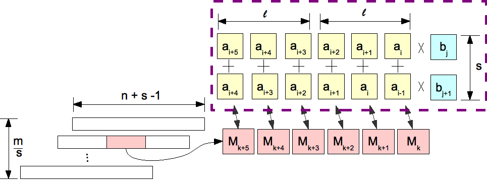
Figure 4: Multiplication phase: illustration of a thread-block reading coefficients from $a$,$b$ and writing to the auxiliary array $M$.

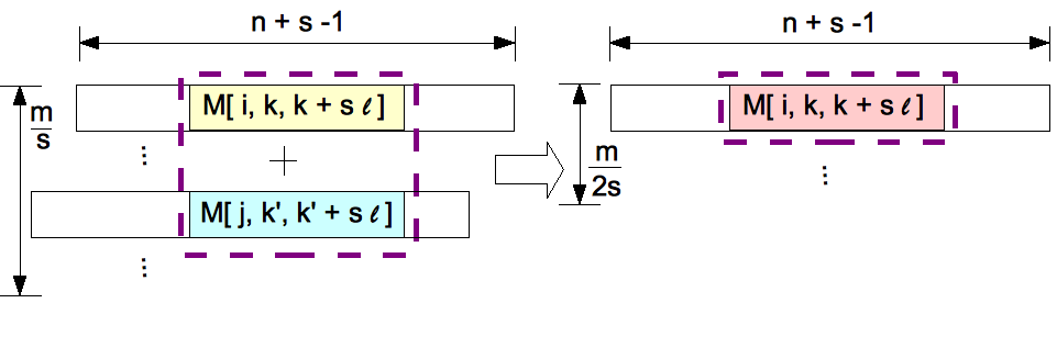
Figure 5: Addition phase: illustration of a thread-block reading and writing to the auxiliary array $M$.

1

Input: $a,b\in{\mathbb{K}}[X]$ with $n-1:={\deg}(a)$ and $m-1:={deg}(b)$ and an integer $s\geq 1$.

2

Output: $f\in{\mathbb{K}}[X]$ and $f=a\times b$.

3

4$y=n+s-1$; $x=m/s$;

5

6Let $M$ be an array of size $x\cdot y$ with coefficients in $\mathbb{K}$;

7

8$\ell$ is the number of threads per block;

9

10MulKer$\lll x\cdot y/(s\cdot{\ell}),\ell\ggg(a,b,M,n,m,s)$;

11 for ($i=0;i\leq\log_{2}{s};i=i+1$) do

12       AddKer$\lll x\cdot y/(2^{i+1}\,s\cdot{\ell}),\ell\ggg(M,f,y,s,x,i)$;

13      

14 return $f$;

Algorithm 5 PlainMultiplicationGPU($a,b,f,s$)

1

Input: $a,b,M\in{\mathbb{K}}[X]$ and an integer $s\geq 1$.

2

3${\ell}=$ blockDim; $t=$ threadID; $j=$blockID$\cdot{\ell}+t$;

4 Let $B^{\prime}$ and $A^{\prime}$ be two local arrays in $\mathbb{K}$ of size $s$ and ${\ell}\cdot s+s-1$ respectively;

5

/* copying from global */

6 $i=s\cdot\lfloor s\cdot j/(n+s-1)\rfloor+t$;

7 if $i<m\wedge t<s$ then

8       $B^{\prime}[t]=b[i]$;

9      

10 $i=s\cdot(j\mod\frac{n+s-1}{s})$;

11 for ($k=0;k<s;k=k+1$) do

12       if $i+k\cdot{\ell}+t<n$ then

13             $A^{\prime}[k\cdot{\ell}+t]=a[i+k\cdot{\ell}+t]$;

14            

15      

16 if $i-s+t>0\wedge t<s-1$ then

17       $A^{\prime}[{\ell}\cdot s+t]=a[i-s+t]$;

18      

19 else if $t<s-1$ then

20       $A^{\prime}[{\ell}\cdot s+t]=0$;

21      

22

23for ($e=0;e<s;e=e+1$) do

24       $h=0$;

25       for ($k=0;k<s;k=k+1$) do

26             $h$ += $A^{\prime}[e\cdot{\ell}+k]\cdot B^{\prime}[k]$;

27            

       /* writing to global memory */

28       $M[s\cdot j+e]=h$;

29      

30

Algorithm 6 MulKer$(a,b,M,n,m,s)$

Input: $M,f,\in{\mathbb{K}}[X]$ and $y,s,x,i$ are positive integers.

1

2$j=$blockID$\cdot$blockDim + threadID;

3 $h=s\cdot j\mod y$;

4 $k=2^{i}-1+2^{i+1}\,\lfloor s\cdot j/y\rfloor$;

5

6if $h<2^{i}\,s$ then

7       for ($e=0;e<s;e=e+1$) do

8             $f[k\cdot s+h+e]$ += $M[k\cdot x+h+e]$;

9            

10      

11 else

12       for ($e=0;e<s;e=e+1$) do

13             $M[(k+2^{i})\cdot x+h-2^{i}\,s+e]$ += $M[k\cdot x+h+e]$;

14            

15      

16

Algorithm 7 AddKer$(M,f,y,s,x,i)$

Considering any thread-block of the multiplication phase, we notice that $s$ coefficients of $b$ and $s\,{\ell}+s-1$ coefficients of $a$ are loaded and $s\,{\ell}$ results are written back to global memory. Hence $2\,s\,{\ell}+2\,s-1$ coefficients must fit into local memory, that is, we have $2\,s\,{\ell}+2\,s-1\leq Z$. Next, we compute the work, span and parallelism overhead, respectively as $W_{s}=(2\,m-\frac{1}{2})\,(n+s-1)$, $S_{s}=2\,s^{2}+s\,\log_{2}\frac{m}{s}-s$ and $O_{s}=\frac{(n+s-1)\,(5\,m\,s+2\,m-3\,s^{2})\,U}{s^{2}\,{\ell}}$. We also obtain the quantities characterizing the thread block DAG that are required in order to apply Corollary 1: $N_{s}=\frac{(n+s-1)\,(2\,m-s)}{s^{2}\,{\ell}}$, $L_{s}=\log_{2}\frac{m}{s}+1$ and $C_{s}=s\,(2\,s-1)+2\,U\,(s+1)$.

We set $s=1$ in Algorithm 5, and view it as a “naive algorithm”. The work ratio $W_{1}/W_{s}={\frac{n}{n+s-1}}$, is asymptotically constant as $n$ escapes to infinity. The span ratio $S_{1}/S_{s}=\frac{\log_{2}{m}+1}{s\,(\log_{2}{(m/s)}+2\,s-1)}$ shows that $S_{s}$ grows asymptotically with $s$. The parallelism overhead ratio, letting $m=n$:

$$\frac{O_{1}}{O_{s}}=\frac{n\,s^{2}\,(7\,n-3)}{(n+s-1)\,(5\,n\,s+2\,n-3\,s^{2})}.$$ (11)

We observe that, as $n$ escape to infinity, this latter ratio is asymptotically equivalent to $s$. Applying Corollary 1, let $R$ be the ratio of the running time estimate between the naive algorithm and that for an arbitrary $s$. We obtain

$$R=\frac{(n\,\log_{2}{n}+3\,n-1)\,(1+4\,U)}{(n\,\log_{2}{\frac{n}{s}}+3\,n-s)\,(2\,U\,s+2\,U+2\,s^{2}-s)},$$ (12)

which is essentially $\frac{2\log_{2}{n}}{s\,\log_{2}{(n/s)}}$. This latter ratio is smaller than $1$, such that the “initial” algorithm (that is for $s=1$) performs better. This also indicates that increasing $s$ makes the algorithm performance worse. In practice shown in Table 1, setting $s=4$ performs best, while with larger $s$, the running time becomes slower, which is coherent with our theoretical analysis.

6 The Euclidean algorithm
for polynomials

Let $a$ and $b$ be polynomials as defined in Section 3. In Section 6.1, we present a simple multithreaded algorithm that computes GCD$(a,b)$ on an MMM machine. We call it naive (like Algorithm 1) as this algorithm also performs one division step within one kernel. In Section 6.2, we describe another algorithm on an MMM machine that reduces the overhead of data transfer by performing several division steps within one kernel. Finally, in Section 6.3 we compare those two algorithms by means of Corollary 1. A detailed analysis in the form of executable Maple worksheet is available at.

6.1 Naive algorithm

Algorithm 8 computes GCD$(a,b)$. Similarly to the naive division of Algorithm 1, it calls a kernel (stated as Algorithm 9) that completes one division step. The former algorithm calls the latter one at most $n+m-2$ times. Algorithm 9 is the same as Algorithm 2 except that it checks the current degrees of both $a$ and $b$ so as to decide which one takes the role of the divisor, and then it completes a division step. To do so, we use an array st of length $2$ to store the degrees of $a$ and $b$ during each division step. The fact that the degree of an intermediate remainder may be dropped by more than $1$ is taken into account, so that Algorithm 9 works correctly even if the GCD is computed before $n+m-2$ kernel calls. After $n+m-2$ division steps, either $a$ or $b$ becomes zero or constant. Algorithm 8 returns the other polynomial as GCD. Figure 6 shows one Euclidean division step within a thread-block after running Algorithm 9 once.

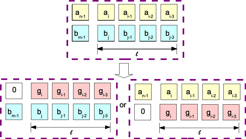
Figure 6: Naive Euclidean: illustration of a thread-block reading coefficients from $a$,$b$ and writing to $g$.

We denote by ${\ell}$ the number of threads per thread-block. We compute the work, span and overhead, respectively as $W_{1}=\frac{m\,(2\,n\,{\ell}+n+\ell-1)}{\ell}$, $S_{1}=3\,(m+n-2)$ and $O_{1}=\frac{5\,m\,U\,(n+\ell+1)}{\ell}$. To apply Corollary 1, one can easily check that those three quantities are $N_{1}=\frac{m\,(n+\ell+1)}{\ell}$, $L_{1}=m+n-2$ and $C_{1}=3+5\,U$.

1

Input: $a,b\in{\mathbb{K}}[X]$ with ${\deg}(a)\geq{\deg}(b)$ that is, $n-1\geq m-1$.

Output: $g\in{\mathbb{K}}[X]$, s.t. $g=$GCD$(a,b)$.

2

3int st$[]=\{\deg(a),\deg(b)\}$;

4Let $\ell$ be the number of threads in a thread block;

5

6for $(i=0;i<n+m-2;i=i+1)$ do

7       NaivePlainGcdKernel$\lll\lceil m/\ell\rceil,\ell\ggg(a,b,$ st);

8      

9

10if $a$ is a zero or constant polynomial then

11       Compute $k_{b}$ the maximum $i$ s.t. $b[i]\neq 0$ holds;

12       Let $g$ be array of size $k_{b}+1$ with coefficients in $\mathbb{K}$ s.t. $g[i]=b[i]$ for $0\leq i\leq k_{b}$;

13      

14else

15       Compute $k_{a}$ the maximum $i$ s.t. $a[i]\neq 0$ holds;

16       Let $g$ be array of size $k_{a}+1$ with coefficients in $\mathbb{K}$ s.t. $g[i]=a[i]$ for $0\leq i\leq k_{a}$;

17      

18 return $g$;

19

Algorithm 8 NaivePlainGcdGPU($a,b$)

1

Input: $a,b\in{\mathbb{K}}[X]$ and st$[]$ stores the current degree of $a$ and $b$.

2$j=$blockID$\cdot$blockDim $+$ threadID;

3

4if st$[0]\geq$ st$[1]>0\wedge j<$ st$[1]$ then

5       $k=j+$st$[0]-$st$[1]$;

6       $a[k]=a[k]-b[j]\cdot a[$st$[0]]\cdot b[$st$[1]]^{-1}$;

7       if $j==$ st$[1]-1$ then

8             while $({\sf st}[0]\geq 0)\wedge(a[{\sf st}[0]]=0)$ do

9                   st$[0]=$ st$[0]-1$;

10                  

11            

12      

13 else if $0<$ st$[0]<$ st$[1]\wedge j<$ st$[0]$ then

14       $k=j+$st$[1]-$st$[0]$;

15       $b[k]=b[k]-a[j]\cdot b[$st$[1]]\cdot a[$st$[0]]^{-1}$;

16      

17      if $j==$ st$[0]-1$ then

18             while $({\sf st}[1]\geq 0)\wedge(b[{\sf st}[1]]=0)$ do

19                   st$[1]=$ st$[1]-1$;

20                  

21            

22      

23

Algorithm 9 NaivePlainGcdKernel($a,b,$ st )

6.2 Optimized algorithm

In each kernel, thread-blocks collectively perform at most $s$ division steps, instead of one, and update $s$ coefficients from both $a$ and $b$. After a division step, the degree of the dividend polynomial is decreased by at least one, and then in the next division step, coefficients from the divisor polynomial are adjusted by one or more shift operations. Thus, we need $2\,s$ coefficients from both $a$ and $b$ to be sure that after $s$ division steps we correctly have $s$ coefficients of both $a$ and $b$. Since the consecutive thread-blocks have $s$ common coefficients of both $a$ and $b$, the number of thread-blocks is $\min(\frac{\deg(a)+1}{s},\frac{\deg(b)+1}{s})$. A thread-block also needs $s$-head coefficients of both $a$ and $b$ to run $s$ division steps. Thus, each thread-block uses $3\,s$ threads (like Algorithm 4). Algorithm 10 is our top level optimized algorithm for computing GCD($a$, $b$). Figure 7 shows $s$ Euclidean division steps within a thread-block after running the kernel Algorithm 11 once.

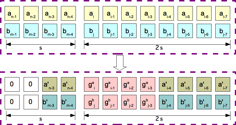
Figure 7: Optimized Euclidean: illustration of a thread-block reading coefficients from $a$,$b$ and writing to $g^{a}$,$g^{b}$.

We compute the work, span and overhead, respectively as $W_{s}=(\frac{9}{4}+\frac{6}{s})\,{m}^{2}+\left(\frac{9}{2}\,n+{\frac{n}{2\,s}}+{\frac{87}{8}}\,s+\frac{23}{2}\right)m-{\frac{345}{16}}\,{s}^{2}-{\frac{77}{4}}\,s$, $S_{s}=3\,n+3\,m$ and $O_{s}=\frac{8\,m\,U\,(n+s)}{s^{2}}$. To apply Corollary 1, one can easily check that those three quantities are $N_{s}=\frac{m\,n}{s^{2}}+\frac{m}{s}$, $L_{s}=\frac{n}{s}+\frac{m}{s}$ and $C_{s}=3\,s+8\,U$.

Input: $a,b\in{\mathbb{K}}[X]$ with ${\deg}(a)\geq{\deg}(b)$ that is, $n-1\geq m-1$ and an integer $s>1$.

Output: $g\in{\mathbb{K}}[X]$, s.t. $g=$GCD$(a,b)$.

1

2int st$[2]=\{\deg(a),\deg(b)\}$;

3 Let $\ell=3s$ be the number of threads in a thread block;

4

5for $(i=0;i<{n+m-2};i=i+s)$ do

6       OptGcdKer$\lll\lceil m/s\rceil,\ell\ggg(a,b,s,$ st);

7      

8

9if $a$ is a zero or constant polynomial then

10       Compute $k_{b}$ the maximum $i$ s.t. $b[i]\neq 0$ holds;

11       Let $g$ be array of size $k_{b}+1$ with coefficients in $\mathbb{K}$ s.t. $g[i]=b[i]$ for $0\leq i\leq k_{b}$;

12      

13else

14       Compute $k_{a}$ the maximum $i$ s.t. $a[i]\neq 0$ holds;

15       Let $g$ be array of size $k_{a}+1$ with coefficients in $\mathbb{K}$ s.t. $g[i]=a[i]$ for $0\leq i\leq k_{a}$;

16      

17 return $g$;

18

Algorithm 10 OptimizedPlainGcdGPU($a,b,s$)

Input: $a,b\in{\mathbb{K}}[X]$, an integer $s>1$ and st$[]$ stores the current degree of $a$ and $b$.

1

2Let sAc, sBc, sA, sB be local arrays of size $s,s,2s,2s$ respectively with coefficients in $\mathbb{K}$;

3

4local integers $u=v=w=e=0$;

5$j=$blockID$\cdot$blockDim $+$ threadID; $t=$ threadID;

6

/* copying from global memory */

7if $t<s$ then

8       sAc$[t]=a[$st$[0]-t]$;

9       sBc$[t]=b[$st$[1]-t]$;

10      

11

12if $t\geq s$ then

13       sA$[t-s]=a[$st$[0]-s\,$blockID$-t]$ sB$[t-s]=b[$st$[1]-s\,$blockID$-t]$;

14      

15

16for $(k=0;k<s;k=k+1)$ do

17       if (st$[0]\geq$st$[1]\wedge$st$[1]\geq 0$) then

18            

19            if $(u+t<s)\wedge(v+t<s)$ then

20                   sAc$[u+t]$ -= sBc$[v+t]\cdot$sAc$[u]\cdot$sBc$[v]^{-1}$;

21                  

22             if $(u+t\geq s)\wedge(v+t\geq s)$ then

23                   sA$[w+t-s]$ -= sB$[e+t-s]\cdot$sAc$[u]\cdot$sBc$[v]^{-1}$;

24                  

25             if $t==0$ then

26                   while sAc$[u]=0$ do

27                         $u=u+1$; $w=w+1$; st$[0]=$st$[0]-1$;

28                        

29                  

30            

31       if (st$[1]\geq$st$[0])\wedge($st$[0]\geq 0)$ then

32            

33            if $(u+t<s)\wedge(v+t<s)$ then

34                   sBc$[v+t]$ -= sAc$[u+t]\cdot$sBc$[v]\cdot$sAc$[u]^{-1}$;

35                  

36             if $(u+t\geq s)\wedge(v+t\geq s)$ then

37                   sB$[e+t-s]$ -= sA$[w+t-s]\cdot$sBc$[v]\cdot$sAc$[u]^{-1}$;

38                  

39            

40            if $t==0$ then

41                   while sBc$[v]=0$ do

42                         $v=v+1$; $e=e+1$; st$[1]=$st$[1]-1$;

43                        

44                  

45            

46      

47

48if $t\geq s$ then

       /* writing to global memory */

49       $a[$st$[0]-s\,$blockID$-t]=$ sA$[t-s]$;

50       $b[$st$[1]-s\,$blockID$-t]=$ sB$[t-s]$ ;

51      

52 if $j==\min($st$[0]$, st$[1])$ then

53       Update st array with the new degree of $a$ and $b$;

54      

Algorithm 11 OptGcdKer($a,b,s$ st)

6.3 Comparison of running time estimates

Since we have $2{\ell}\leq Z$ and $6s\leq Z$, we replace ${\ell}$ and $s$ by $Z/2$ and $Z/6$, respectively, and assume that $m$ equals to $n$. We first observe that the ratio $W_{1}/W_{s}$ is asymptotically constant, essentially ${\frac{8\,(Z+1)}{3\,(9\,Z+52)}}$, and the span ratio $S_{1}/S_{s}=\frac{n+m-2}{n+m}$ is asymptotically 1. Next, we compute the overhead ratio $O_{1}/O_{s}$, that is,

$$\frac{O_{1}}{O_{s}}={\frac{5}{48}}\,{\frac{Z\left(2\,n+2+Z\right)}{6\,n+Z}}.$$ (13)

We see that the parallelism overhead improvement is done at a fairly low expense in terms of work overhead. Applying Corollary 1, we denote the running time estimate ratio $R$ of the naive algorithm over the optimized one, that is,

$$R={\frac{\left(6\,n-2+Z\right)\left(3+5\,U\right)Z}{\left(18\,n+Z\right)\left(Z+16\,U\right)}}.$$ (14)

When $n$ escapes to infinity, the ratio $R$ is equivalent to

$$\frac{(3+5\,U)\,Z}{3\,(Z+16\,U)}.$$ (15)

We observe that this ratio is larger than $1$ if and only if $Z>9.6$ holds. This condition clearly holds and the optimized algorithm is overall better. This is verified in practice [9], where $s$ is set to $256$, also shown in Table 2.

$n$	$m$	$s$ = 2	$s$ = 4	$s$ = 8	$s$ = 16
4000	4000	0.004107	0.002775	0.003727	0.004811
5000	1000	0.001684	0.001204	0.001432	0.003645
5000	5000	0.008007	0.005846	0.007808	0.011715
6000	1000	0.001830	0.001298	0.001500	0.004129
6000	6000	0.010359	0.007614	0.010166	0.014352
7000	1000	0.001972	0.001381	0.001614	0.004551
7000	7000	0.013068	0.008821	0.012166	0.016938
8000	1000	0.002111	0.001456	0.001739	0.005015
8000	8000	0.016029	0.010853	0.014877	0.019740

Table 1: Running time (secs) of the polynomial multiplication algorithm with polynomials $a$ ($\deg(a)=n-1$) and $b$ ($\deg(b)=m-1$) and the parameter $s$

$n$	$m$	$s$ = 1	$s$ = 512
2000	1500	0.058	0.024
3000	2500	0.108	0.039
4000	3500	0.158	0.053
5000	4500	0.203	0.069
6000	5000	0.235	0.056
7000	6000	0.282	0.066
8000	7000	0.324	0.076
9000	8000	0.367	0.087
10000	9000	0.411	0.097

Table 2: Running time (secs) of the Euclidean algorithm for polynomials $a$ ($\deg(a)=n-1$) and $b$ ($\deg(b)=m-1$) with the parameter $s$

7 Conclusion

We have presented a model of multithreaded computation combining the fork-join and SIMD parallelisms, with an emphasis on estimating parallelism overheads, so as to reduce communication and synchronization costs in GPU programs.

Four applications illustrated the effectiveness of our model. In each case, we determined a range of values for a program parameter in order to optimize the corresponding algorithm in terms of parallelism overheads. Experimentation validated the model prediction.

Our order of magnitude estimates for the program parameter of radix sort [19] agrees with the empirical results of that paper.

For the Euclidean algorithm, our running time estimates match those obtained with the Systolic VLSI Array Model [3]. Moreover, our CUDA code [9] implementing this optimized Euclidean algorithm runs in linear time w.r.t to the input polynomials degree, up to degree 10,000.

For polynomial multiplication, our theoretical analysis implies that the program parameter $s$ must be as small as possible. In practice, we could vary this parameter between $2$ and $32$ and we found that the optimal value was $4$. Since certain hardware features are not integrated into the model, we found that the model prediction was also useful in that case.

References

- [1] R. D. Blumofe and C. E. Leiserson. Space-efficient scheduling of multithreaded computations. SIAM J. Comput., 27(1):202–229, 1998.
- [2] R. D. Blumofe and C. E. Leiserson. Scheduling multithreaded computations by work stealing. J. ACM, 46(5):720–748, 1999.
- [3] R. P. Brent and H. T. Kung. Systolic VLSI arrays for polynomial GCD computation. IEEE Trans. Computers, 33(8):731–736, 1984.
- [4] M. Frigo, C. E. Leiserson, H. Prokop, and S. Ramachandran. Cache-oblivious algorithms. In FOCS, pages 285–298, 1999.
- [5] P. B. Gibbons. A more practical PRAM model. In Proc. of SPAA, pages 158–168, 1989.
- [6] P. B. Gibbons, Y. Matias, and V. Ramachandran. The Queue-Read Queue-Write PRAM model: Accounting for contention in parallel algorithms. SIAM J. on Comput., 28(2):733–769, 1998.
- [7] R. L. Graham. Bounds on multiprocessing timing anomalies. SIAM J. on Applied Mathematics, 17(2):416–429, 1969.
- [8] T. D. Han and T. S. Abdelrahman. Reducing branch divergence in GPU programs. In Proc. of GPGPU-4, pages 3:1–3:8, 2011.
- [9] S. A. Haque and M. Moreno Maza. Plain polynomial arithmetic on GPU. In J. of Physics: Conf. Series, volume 385, page 12014. IOP Publishing, 2012.
- [10] Y. He, C. E. Leiserson, and W. M. Leiserson. The Cilkview scalability analyzer. In Proc. of SPAA, pages 145–156, 2010.
- [11] C. E. Leiserson. The cilk++ concurrency platform. The Journal of Supercomputing, 51(3):244–257, 2010.
- [12] W. Liu, W. Muller-Wittig, and B. Schmidt. Performance predictions for general-purpose computation on GPUs. In Proc. of ICPP, page 50, 2007.
- [13] L. Ma, K. Agrawal, and R. D. Chamberlain. A memory access model for highly-threaded many-core architectures. In Proc. of ICPADS, pages 339–347, 2012.
- [14] L. Ma and R. D. Chamberlain. A performance model for memory bandwidth constrained applications on graphics engines. In Proc. of ASAP, pages 24–31. IEEE Computer Society, 2012.
- [15] L. Mirsky. A dual of Dilworth’s decomposition theorem. The American Math. Monthly, 78(8):876–877, 1971.
- [16] J. Nickolls, I. Buck, M. Garland, and K. Skadron. Scalable parallel programming with CUDA. Queue, 6(2):40–53, 2008.
- [17] C. NVIDIA. NVIDIA next generation CUDA compute architecture: Kepler GK110, 2012.
- [18] A. D. Robison. Composable parallel patterns with Intel Cilk Plus. Computing in Science & Engineering, 15(2):0066–71, 2013.
- [19] N. Satish, M. Harris, and M. Garland. Designing efficient sorting algorithms for manycore GPUs. In Proc. of IPDPS 2009, pages 1–10. IEEE, 2009.
- [20] J. Shin. Introducing control flow into vectorized code. In Proceedings of the 16th International Conference on Parallel Architecture and Compilation Techniques, PACT ’07, pages 280–291, Washington, DC, USA, 2007. IEEE Computer Society.
- [21] L. J. Stockmeyer and U. Vishkin. Simulation of parallel random access machines by circuits. SIAM J. Comput., 13(2):409–422, 1984.
- [22] J. E. Stone, D. Gohara, and G. Shi. OpenCL: A parallel programming standard for heterogeneous computing systems. Computing in science & engineering, 12(3):66, 2010.