Graph Cuts with Interacting Edge Costs – Examples, Approximations, and Algorithms

Abstract

We study an extension of the classical graph cut problem, wherein we replace the modular (sum of edge weights) cost function by a submodular set function defined over graph edges. Special cases of this problem have appeared in different applications in signal processing, machine learning, and computer vision. In this paper, we connect these applications via the generic formulation of “cooperative graph cuts”, for which we study complexity, algorithms, and connections to polymatroidal network flows. Finally, we compare the proposed algorithms empirically.

1 Introduction

Graphs have been a ubiquitous modeling tool in areas as diverse as operations research, signal processing and machine learning. Graphical representations reveal structure in the problem that is often the key to obtaining efficient algorithms for real-world data analysis problems. As a prominent example, the Minimum $(s,t)$-Cut problem underlies important problems in low-level computer vision (Boykov and Veksler, 2006) (e.g., image segmentation and regularization), probabilistic inference in graphical models (Greig et al., 1989; Ramalingam et al., 2008), and for representing pseudo-boolean functions in computer vision and constraint satisfaction problems (Kolmogorov and Boykov, 2005; Ramalingam et al., 2011; Z̆ivný et al., 2009). The reduction to cuts has had a tremendous practical impact.

The algorithmic efficiency of cuts comes at the price of reduced modeling power: graph cuts model problems that correspond to a special class of functions (a sub-class of submodular functions defined on the nodes of the graph (Z̆ivný et al., 2009)). Section 2 lists applications that do not fall into this category. Motivated by these limitations, this paper studies a non-additive generalization of Minimum $(s,t)$-Cut, where the cut cost function is a submodular set function over graph edges.

A set function $f:2^{\mathcal{E}}\to\mathbb{R}$ defined on subsets of a ground set $\mathcal{E}$ is submodular if it satisfies diminishing marginal costs: for all sets $A\subset B\subseteq\mathcal{E}$ and $e\in\mathcal{E}\setminus B$, it holds that

$$f(A\cup\{e\})-f(A)\geq f(B\cup\{e\})-f(B).$$ (1)

This generalization – we refer to it as Cooperative Cut – introduces dependencies between edges, and expresses a wider set of functions than graph cuts.

1.1 Minimum Cut and Minimum Cooperative Cut

The Minimum $(s,t)$-Cut problem is defined as follows.

Problem 1 (Minimum $(s,t)$-Cut).

Given a weighted graph $\mathcal{G}=(\mathcal{V},\mathcal{E},w)$ with terminal nodes $s,t\in\mathcal{V}$, find a cut $C\subseteq\mathcal{E}$ of minimum cost $w(C)=\sum_{e\in C}w(e)$. A cut is a set of edges whose removal disconnects all paths between $s$ and $t$.

We assume throughout that $w\geq 0$. Many very efficient algorithms are known to solve Minimum $(s,t)$-Cut; the reader is referred to (Ahuja et al., 1993; Schrijver, 2004) for an overview.

In graph cuts, the cost of any given cut $C\subseteq\mathcal{E}$ is a sum $w(C)=\sum_{e\in C}w(e)$ of edge weights. This function is said to be modular or, equivalently, additive on the edge set $\mathcal{E}$. It implies two important modeling characteristics for graph cuts: First, the nonnegativity of the weights can only penalize two nodes for being separated — this introduces a form of positive correlation between nodes, also hence this is sometimes referred to as attractive potentials in the computer vision community. Second, modular edge weights express interactions of only two nodes at a time. That is, the additive contribution $w(e)$ to the cost $\sum_{e\in C}w(e)$ of a cut $C$ by a given edge $e\in C$ is the same regardless of the cut in which the edge $e$ is considered.

Several applications, however, are more accurately modeled when allowing non-additive interactions between edge weights. We survey some examples and applications in Section 2. These examples are captured when replacing the modular cost function $w$ by a nonnegative and nondecreasing submodular set function over graph edges. The definition (1) implies that with submodular edge weights, the cost of an additional edge depends on which other edges are contained in the cut. This non-additivity allows specific long-range dependencies between multiple (pairs of) nodes simultaneously that cannot be expressed by graph cuts. These observations motivate the definition of cooperative graph cuts.

Problem 2 (Minimum cooperative cut (MinCoopCut)).

Given a graph $\mathcal{G}=(\mathcal{V},\mathcal{E},f)$ with terminal nodes $s,t\in\mathcal{V}$ and a nonnegative, monotone nondecreasing submodular function $f:2^{\mathcal{E}}\to\mathbb{R}_{+}$ defined on subsets of edges, find an $(s,t)$-cut $C\subseteq\mathcal{E}$ of minimum cost $f(C)$.

A set function $f$ is nondecreasing if $A\subseteq B\subseteq\mathcal{E}$ implies that $f(A)\leq f(B)$. MinCoopCut is a constrained submodular minimization problem:

$$\text{minimize }f(C)\quad\text{ subject to }C\subseteq\mathcal{E}\text{ is an $(s,t)$-cut in }\mathcal{G}.$$ (2)

As cooperative cuts employ the same graph structures as standard graph cuts, they easily integrate into and extend many of the applications of graph cuts. We note, however, that the graph $\mathcal{G}$ need not have any relationship to the submodular function $f$ other than the fact that the edges of the graph $\mathcal{G}$ constitute the ground set of $f$.

1.2 Relation to the literature

Cooperative graph cuts relate to the recent literature in two aspects. First, a number of models in signal processing, computer vision, security, and machine learning are special cases of cooperative cuts, as is discussed in Section 2.

Second, recent interest has emerged in the literature regarding the implications of extending classical combinatorial problems (such as Shortest Path, Minimum Spanning Tree, or Set Cover) from a sum-of-weights to submodular cost functions (Svitkina and Fleischer, 2008; Iwata and Nagano, 2009; Goel et al., 2009, 2010; Jegelka and Bilmes, 2011a, b; Koufogiannakis and Young, 2009; Hassin et al., 2007; Zhang et al., 2011; Baumann et al., 2013). None of this work, however, has addressed cuts. In this work, we provide lower and upper bounds on the approximation factor of MinCoopCut.

One approach to solving MinCoopCut is via relaxations. For Minimum $(s,t)$-Cut, a celebrated result of (Ford and Fulkerson, 1956; Dantzig and Fulkerson, 1955) states that the dual of the linear programming relaxation is a Maximum Flow problem, and that their optimal values coincide. We refer to the ratio between the maximum flow value (i.e., the optimal value of the relaxation), and the optimal value of the discrete cut, as the flow-cut gap. For Minimum $(s,t)$-Cut, this ratio is one. In Section 4, we formulate a convex relaxation of MinCoopCut whose dual problem is a generalized flow problem, where submodular capacity constraints are placed not only on individual edges but on arbitrary sets of edges simultaneously. The flow-cut gap for this problem can be on the order of $n$, the number of nodes. In contrast, the related polymatroidal maximum flow problem (Lawler and Martel, 1982; Hassin, 1982) (defined in Section 5.1.3) still has a flow-cut gap of one. Polymatroidal flows are equivalent to submodular flows, and have recently gained attention for modeling information flow in wireless networks (Kannan et al., 2011; Kannan and Viswanath, 2011; Chekuri et al., 2012). Their dual problem is a minimum cut problem where the edge weights are defined by a convolution of local submodular functions (Lovász, 1983). Such convolutions are generally not submodular (see Equation (28)).

1.3 Summary of main contributions

In this paper, we survey diverse examples of cooperative cuts in different applications, and provide a detailed theoretical analysis:

• We show a lower bound of $\Omega(\sqrt{n})$ on the approximation factor for the general MinCoopCut problem.

• We analyze two families of approximation algorithms. The first relies on substituting the submodular cost function by a tractable approximation. The second family consists of rounding algorithms that build on the relaxation of the problem. Both families contain algorithms that use a partitioning of edges into node incidence sets, but in different ways.

• We provide a lower bound of $n-1$ on the flow-cut gap, and relate it to different families of submodular functions.

In Section 5.1.3 we draw connections to polymatroidal flows (Lawler and Martel, 1982; Hassin, 1982). The non-additive cut cost function used in the resulting approximation is solvable exactly and may itself be interesting to consider as an exactly solvable class of e.g. higher-order potentials in computer vision. The paper concludes with a discussion of open problems. In particular, the results of this paper motivate a wider and more refined study of the complexity and expressive power of non-additive graph cut problems.

The paper is structured as follows. In Section 2 we discuss various instances of cooperative cuts and their properties. The complexity of MinCoopCut is addressed in Section 3, convex relaxations in Section 4, and algorithmic approaches in Section 5.

1.4 Notation and technical preliminaries

Throughout this paper, we are given a directed graph $\mathcal{G}=(\mathcal{V},\mathcal{E})$ with $n$ nodes and $m$ edges, and terminal nodes $s,t\in\mathcal{V}$. The function $f:2^{\mathcal{E}}\to\mathbb{R}_{+}$ is submodular and monotone nondecreasing, where by $2^{\mathcal{E}}$ we denote the power set of $\mathcal{E}$. We assume $f$ to be normalized, i.e., $f(\emptyset)=0$. Equivalently to Definition (1), the function $f$ is submodular if for all $A,B\subseteq\mathcal{E}$, it holds that

$$f(A)+f(B)\geq f(A\cup B)+f(A\cap B).$$ (3)

The function $f$ generalizes commonly used modular edge weight functions $w:\mathcal{E}\to\mathbb{R}_{+}$ that satisfy Equation 3 with equality. We denote the marginal cost of an element $e\in\mathcal{E}$ with respect to a set $A\subseteq\mathcal{E}$ by $f(e\mid A)\triangleq f(A\cup\{e\})-f(A)$. A function $f(A)=g(w(A))$ for a nonnegative modular function $w$ and a concave scalar function $g$ is always submodular.

For any node $v\in\mathcal{V}$, let $\delta^{+}(v)=\{(v,u)\in\mathcal{E}\}$ be the set of edges directed out of $v$, and $\delta^{-}(v)=\{(u,v)\in\mathcal{E}\}$ be the set of edges into $v$. Together, these two directed sets form the (undirected) incidence set $\delta(v)=\delta^{+}(v)\cup\delta^{-}(v)$. These definitions directly extend to sets of nodes: for a set $S\subseteq\mathcal{V}$ of nodes, $\delta^{+}(S)=\{(v,u)\in\mathcal{E}:v\in S,u\notin S\}$ is the set of edges leaving $S$. Without loss of generality, we assume all graphs are simple.

The Lovász extension $\tilde{f}:[0,1]^{m}\to\mathbb{R}$ of the submodular function $f$ is its lower convex envelope and is defined as follows (Lovász, 1983). Given a vector $x\in[0,1]^{m}$, we can uniquely decompose $x$ into its level sets $\{B_{j}\}_{j}$ as $x=\sum_{j}\lambda_{j}\chi_{B_{j}}$ where $B_{1}\subset B_{2}\subset\dots$ are distinct subsets. Here and in the following, $\chi_{B}\in[0,1]^{m}$ is the characteristic vector of the set $B$, with $\chi_{B}(e)=1$ if $e\in B$, and $\chi_{B}(e)=0$ otherwise. Then $\tilde{f}(x)=\sum_{j}\lambda_{j}f(B_{j})$. This construction illustrates that $\tilde{f}(\chi_{B})=f(B)$ for any set $B$. The Lovász extension can be computed by sorting the entries of the argument $x$ in $O(m\log m)$ time and calling $f$ $m$ times.

A separator of a submodular function $f$ is a set $S\subseteq\mathcal{E}$ with the property that $f(S)+f(\mathcal{E}\setminus S)=f(\mathcal{E})$, implying that for any $B\subseteq\mathcal{E}$, $f(B)=f(B\cap S)+f(B\cap(\mathcal{E}\setminus S))$. If $S$ is a minimal separator, then we say that $f$ couples all edges in $S$. For the edges within a minimal separator, $f$ is strictly subadditive: $\sum_{e\in S}f(e)>f(S)$ for $|S|>1$. That means, the joint cost of this set of edges is smaller than the sum of their individual costs.

1.5 Node functions induced by submodular edge weights

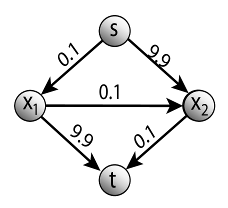
Let $f(A)=\sqrt{\sum_{e\in A}w(e)}$, so

$h(X)=\sqrt{\sum_{e\in\delta^{+}(X)}w(e)}$.

Then $h$ is not submodular:

$$h(\{s,x_{1}\})+h(\{s,x_{2}\})=\sqrt{19.9}+\sqrt{0.2}\;\;\;<\;\;\;2\sqrt{10}=h(\{s\})+h(\{s,x_{1},x_{2}\})$$

Figure 1: The node function induced by a cooperative cut is in general not submodular. The above $h$ violates inequality (3) for $A=\{s,x_{1}\}$, $B=\{s,x_{2}\}$ but satisfies it (strictly) for $A=\{t,x_{1}\}$, $B=\{t,x_{2}\}$.

Every cost function $f$ on graph edges defines a cut function $h:2^{\mathcal{V}}\to\mathbb{R}_{+}$ on sets $X\subseteq\mathcal{V}$ of nodes:

$$h(X)\triangleq f(\delta^{+}(X)).$$ (4)

It is well known that if $f$ is a (modular) sum of nonnegative edge weights, then $h$ is submodular (Schrijver, 2004). In fact, the following is true:

Proposition 1.

The function $f$ is a non-negative modular function on the edge set if and only if $h(X)=f(\delta^{+}(X))$ is a submodular function on the nodes for all edge-induced sub-graphs of $\mathcal{G}=(\mathcal{V},\mathcal{V}\times\mathcal{V})$.

If, however, $f$ is an arbitrary nondecreasing submodular function, then this is not always the case, as Figure 1 illustrates. Proposition 2, proven in Appendix B, summarizes some key properties of $h$.

Proposition 2.

Let $h:2^{\mathcal{V}}\to\mathbb{R}$, $h(X)\triangleq f(\delta^{+}(X))$ be the node function induced by a cooperative cut with nonnegative nondecreasing submodular cost function $f$. Then:

1. $h$ is not always submodular, and

2. $h$ is subadditive, i.e., $h(A)+h(B)\geq h(A\cup B)$ for any $A,B\subseteq\mathcal{V}$.

The non-submodularity of $h$ shows that cooperative cuts are strictly more general than (modular-weight) graph cuts. In some cases, the function $h$ is submodular. One obvious sufficient condition is that $f$ is nonnegative and modular, but this condition is not necessary as shown in the following.

Proposition 3.

Let $f$ be monotone submodular and permutation symmetric in the sense that $f(A)=f(\sigma(A))$ for any permutation $\sigma$ of the set $\mathcal{E}$. If $\mathcal{G}$ is a complete graph, then $h$ is submodular.

Proof.

Symmetry implies that $f$ is of the form $f(A)=g(|A|)$ for a scalar function $g$. Submodularity of $f$ implies that there is always a function $g^{\prime}$ that interpolates $g$ on $\mathbb{R}\setminus\{0,1,\ldots,m\}$, i.e., $f(A)=g^{\prime}(|A|)=g(|A|)$, and $g^{\prime}$ is a piecewise linear concave function. Let $E_{XY}$ be the edges between sets $X$ and $Y$. The submodularity of $h$ is identical to the condition that for all $X\subseteq\mathcal{V}$, $x,y\notin X$, it holds that

$$h(X\cup x)+h(X\cup y)\geq h(X)+h(X\cup x\cup y).$$ (5)

Let $R=\mathcal{V}\setminus(X\cup x\cup y)$. By the concavity and monotonicity of $g^{\prime}$ we have

$$h(X)+h(X\cup x\cup y)$$

$$\quad=g^{\prime}(|E_{XR}|+|E_{Xx}|+|E_{Xy}|)+g^{\prime}(|E_{XR}|+|E_{Rx}|+|E_{Ry}|)$$

$$\quad=g^{\prime}(|X||R|+2|X|)+g^{\prime}(|X||R|+2|R|)$$

$$\quad\leq 2g^{\prime}(|X||R|+|X|+|R|)$$

$$\quad\leq g^{\prime}(|E_{XR}|+|E_{Xy}|+|E_{Rx}|+|E_{xy}|)+g^{\prime}(|E_{XR}|+|E_{Xx}|+|E_{Ry}|+|E_{xy}|)$$

$$\quad=h(X\cup x)+h(X\cup y),$$

and hence submodularity of $h$ follows. ∎∎

Note that if $\mathcal{G}$ is not complete, then $h$ might no longer be submodular. An exact (possibly algebraic or graph-theoretic) characterization of the conditions on $\mathcal{G}$ and $f$ that imply submodularity of $h$ is currently an open problem.

2 Motivation and special cases

We begin by surveying special cases of cooperative cuts from applications in signal processing, machine learning, and computer vision. Notably, some of these applications lead to submodular node functions $h$ as defined in (4) and are hence polynomial-time solvable, while for others $h$ is not submodular. We first discuss the latter case which motivated this paper, and then special submodular cases. Additional special cases are discussed in Section 6.

2.1 General, non-submodular examples

Image segmentation.

The classical task of segmenting an image into a foreground object and its background is commonly formulated as a maximum a posteriori (MAP) inference problem in a Markov Random Field (MRF) or Conditional Random Field (CRF). If the potential functions of the random field are submodular functions (of the node variables), then the MAP solution can be computed efficiently via the minimum cut in an auxiliary graph (Greig et al., 1989; Boykov and Jolly, 2001; Kolmogorov and Zabih, 2004).

While these graph cut models have been very successful in computer vision, they suffer from known shortcomings. For example, the cut model implicitly penalizes the length of the object boundary, or equivalently the length of a corresponding graph cut around the object. As a result, MAP solutions (minimum cuts) tend to truncate fine parts of an object (such as branches of trees, or animal hair), and to neglect carving out holes (such as the mesh grid of a fan, or written letters on paper). This tendency is aggravated if the image has regions of low contrast, where local information is insufficient to determine correct object boundaries.

A solution to both of these problems is proposed in (Jegelka and Bilmes, 2011a). It relies on the continuation of “obvious” object boundaries: one aims to reduce the cut cost if the cut consists of edges (pairs of pixels) with similar appearance. This aim is impossible to model with a modular-cost graph cut where edges are independent. Hence, Jegelka and Bilmes (2011a) replace the graph cut by a cooperative cut that lowers the cost for sets of similar edges. Specifically, the edges in the image graph are partitioned into groups $S_{i}$ of similar edges, where similarity is defined via the adjacent pixels (nodes), and the cut cost is

$$f(C)=\sum_{i=1}^{k}g_{i}(w(C\cap S_{i})),$$ (6)

where the $g_{i}$ are increasing, strictly concave functions, and $w(C)=\sum_{e\in C}w(e)$ is a sum of nonnegative weights.

From the viewpoint of graphical models, the function $h$ induced by (6) is a higher-order potential, i.e., a polynomial of degree much larger than 2. The model (6) also applies to multi-label (scene labeling) problems and other computer vision tasks (Kohli et al., 2013; Silberman et al., 2014; Taniai et al., 2015).

An alternative cooperative cut function has been studied to improve image segmentation results:

$$f(C)=\max_{e\in C}w(e).$$ (7)

Contrary to the cost function (6), the function (7) couples all edges in the grid graph uniformly, without any similarity constraints or grouping. As a result, the cost of any long cut is discounted. Sinop and Grady (2007) and Allène et al. (2009) derive this function as the $\ell_{\infty}$ norm of the (gradient) vector of pixel differences; this vector is the edge indicator vector $y$ in the relaxation we define in Section 4. Conversely, the relaxation of the cooperative cut problem leads to new, possibly non-uniform and group-structured regularization terms (Jegelka, 2012).

Label Cuts.

In computer security, attack graphs are state graphs modeling the steps of an intrusion. Each transition edge is labeled by an atomic action $a$, and blocking an action $a$ blocks the set of all associated edges $S_{a}\subseteq\mathcal{E}$ that carry label $a$. To prevent an intrusion, one must separate the initial state $s$ from the goal state $t$ by blocking (cutting) appropriate edges. The cost of cutting a set of edges is the cost of blocking the associated actions (labels), and paying for one action $a$ accounts for all edges in $S_{a}$. If each action has a cost $c(a)$, then a minimum label cut that minimizes the submodular cost function

$$f(C)=\sum\nolimits_{a}c(a)\min\{1,|C\cap S_{a}|\}$$ (8)

indicates the lowest-cost prevention of an intrusion (Jha et al., 2002).

Sparse separators of Dynamic Bayesian Networks.

A graphical model $\mathsf{G}=(\mathsf{V},\mathsf{E})$ defines a family of probability distributions. It has a node $\mathsf{v}_{i}$ for each random variable $x_{i}$, and any represented distribution $p(x)$ must factor with respect to the edges of the graph as $p(x)\propto\prod_{(\mathsf{v}_{i},\mathsf{v}_{j})\in\mathsf{E}}\psi_{ij}(x_{i},x_{j})$. A dynamic graphical model (DGM) (Bilmes, 2010) consists of three template parts: a prologue $\mathsf{G}^{p}=(\mathsf{V}^{p},\mathsf{E}^{p})$, a chunk $\mathsf{G}^{c}=(\mathsf{V}^{c},\mathsf{E}^{c})$ and an epilogue $\mathsf{G}^{e}=(\mathsf{V}^{e},\mathsf{E}^{e})$. Given a length $\tau$, an unrolling of the template is a model that begins with $\mathsf{G}^{p}$ on the left, followed by $\tau+1$ repetitions of the “chunk” part $\mathsf{G}^{c}$ and ending in the epilogue $\mathsf{G}^{e}$.

To perform inference efficiently, a periodic section of the partially unrolled model is identified on which an effective inference strategy (e.g., a graph triangulation, an elimination order, or an approximate inference method) is developed and then repeatedly used for the complete duration of the model unrolled to any length. This periodic section has boundaries corresponding to separators in the original model (Bilmes, 2010) which are called the interface separators. Importantly, the efficiency of any inference algorithm derived within the periodic section depends critically on properties of the interface, since the variables within must become a clique.

In general, the computational cost of inference is lower bounded, and the memory cost of inference is exactly given, by the size of the joint state space of the interface variables. A “small” separator corresponds to a minimum vertex cut in the graphical model, where the cost function measures the size of the joint state space. Vertex cuts can be rephrased as standard edge cuts. Often, a modular cost function suffices for good results. Sometimes, however, a more general cost function is needed. In Bilmes and Bartels (2003), for example (which is our original motivation for studying MinCoopCut), a state space function that considers deterministic relationships between variables is found to significantly decrease inference costs.

An example of a function that respects determinism is the following. In a Bayesian network possessing determinism, let $D$ be the subset of fully deterministic nodes. That means any $x_{i}\in D$ is a deterministic function of the variables corresponding to its parent nodes $\mathrm{par}(i)$ meaning $p(x_{i}|x_{\mathrm{par}(i)})=\mathbf{1}[x_{i}=g(x_{\mathrm{par}(i)})]$ for some deterministic function $g$. Let $\mathcal{D}_{i}$ be the state space of variable $x_{i}$. Furthermore, given a set $A$ of variables, let $A_{D}=\{x_{i}\in A\cap D\mid\mathrm{par}(i)\subseteq A\}$ be its subset of fully determined variables. If the state space of a deterministic variable is not restricted by fixing a subset of its parents, then the function measuring the state space of a set of variables $A$ is $f(A)=\prod_{x_{i}\in A\setminus A_{D}}|\mathcal{D}_{i}|$. The logarithm of this function is a submodular function, and therefore the problem of finding a good separator is a cooperative (vertex) cut problem. In fact, this function is a lower bound on the computational complexity of inference, and corresponds exactly to the memory complexity since memory need be retained only at the boundaries between repeated sections in a DGM.

More generally, a similar slicing mechanism applies for partitioning a graph for use on a parallel computer — we may seek separators that require little information to be transferred from one processor to another. A reasonable proxy for such “compressibility” is the entropy of a set of random variables, a well-known submodular function. The resulting optimization problem of finding a minimum-entropy separator is a cooperative cut that is different from any known special cases.

Robust optimization.

Assume we are given a graph where the weight of each edge $e\in\mathcal{E}$ is noisy and distributed as $\mathcal{N}(\mu(e),\sigma^{2}(e))$ for nonnegative mean weights $\mu(e)$. The noise on different edges is independent, and the cost of a cut is the sum of edge weights of an unknown draw from that distribution. In such a case, we might want to not only minimize the expected cost, but also take the variance into consideration. This is the aim in mean-risk minimization (which is equivalent to a probability tail model or value-at-risk model), where we aim to minimize

$$f(C)=\sum_{e\in C}\mu(e)+\lambda\sqrt{\sum_{e\in C}\sigma^{2}(e)}.$$ (9)

This is a cooperative cut, and this special case admits an FPTAS (Nikolova, 2010).

2.2 Special cases that lead to submodular functions $h$

Curiously, some instances of cooperative cuts provably yield submodular node functions $h$ and are hence easier. In the first two examples below, $f$ is defined over edges in a complete graph and is symmetric. Here, symmetry is meant in the sense of (Vondrák, 2013) and Proposition 3, the function is indifferent to permutations of the arguments.

Higher-order potentials in computer vision.

A number of higher-order potentials (pseudo-boolean functions) from computer vision, i.e., potential functions that introduce dependencies between more than two variables at a time, can be reformulated as cooperative cuts. As an example, $P^{n}$ Potts functions (Kohli et al., 2009a) and robust $P^{n}$ potentials (Kohli et al., 2009b) bias image labelings to assign the same label to larger patches of pixels (of uniform appearance). The potential is low if all nodes in a given patch take the same label, and high if a large fraction deviates from the majority label. These potential functions correspond to a complete graph with a cooperative cut cost function

$$f(C)=g(|C|),$$ (10)

for a concave function $g$. The larger the fraction of deviating nodes, the more edges are cut between labels, leading to a higher penalty. The function $g$ makes this robust by capping the maximum penalty.

Regularization and Total Variation.

A popular regularization term in signal processing, and in particular for image denoising, has been the Total Variation (TV) and its discretization (Rudin et al., 1992). The setup commonly includes a pixel variable (say $x_{j}$ or $x_{ij}$) corresponding to each pixel or node in the image graph $\mathcal{G}$, and an objective that consists of a loss term and the regularization. The discrete TV for variables $x_{ij}$ corresponding to pixels $v_{ij}$ in an $M\times M$ grid with coordinates $i,j$ is given as

$$\mathrm{TV}_{1}(x)=\sum_{i,j=1}^{M}\sqrt{(x_{i+1,j}-x_{ij})^{2}+(x_{i,j+1}-x_{ij})^{2}}.$$ (11)

If $x$ is constrained to be a $\{0,1\}$-valued vector, then this is an instance of cooperative cut — the pixels valued at unity correspond to the selected elements $X\subseteq\mathcal{V}$, and the edge submodular function corresponds to $f(C)=\sum_{ij}\sqrt{C\cap S_{ij}}$ for $C\subseteq\mathcal{E}$ where $S_{ij}=\{(v_{i+1,j}v_{ij}),(v_{i,j+1},v_{ij})\}\subseteq\mathcal{E}$ ranges over all relevant neighborhood pairs of edges. Discrete versions of other variants of total variation are also cooperative cuts. Examples include the combinatorial total variation of Couprie et al. (2011):

$$\mathrm{TV}_{2}(x)=\sum_{i}\sqrt{\sum_{(v_{i},v_{j})\in\mathcal{E}}\nu_{i}^{2}(x_{i}-x_{j})^{2}},$$ (12)

and the submodular oscillations in (Chambolle and Darbon, 2009), for instance,

$$\mathrm{TV}_{3}(x) =\sum_{1\leq i,j\leq M}\max\{x_{i,j},x_{i+1,j},x_{i,j+1},x_{i+1,j+1}\}$$

$$\qquad\qquad\qquad-\min\{x_{i,j},x_{i+1,j},x_{i,j+1},x_{i+1,j+1}\}$$ (13)

$$=\sum_{1\leq i,j\leq M}\max_{\ell,r\in U_{ij}\times U_{ij}}|x_{\ell}-x_{k}|,$$ (14)

where for notational convenience we used $U_{ij}=\{(i,j),(i+1,j),(i,j+1),(i+1,j+1)\}$. The latter term (14), like $P^{n}$ potentials, corresponds to a symmetric submodular function on a complete graph, and both (10) and (14) lead to submodular node functions $h(X)$.

Approximate submodular minimization.

Graph cuts have been useful optimization tools but cannot represent any arbitrary set function, not even all submodular functions (Z̆ivný et al., 2009). But, using a decomposition theorem by Cunningham (1983), any submodular function can be phrased as a cooperative graph cut. As a result, any fast algorithm that computes an approximate minimum cooperative cut can be used for (faster) approximate minimization of certain submodular functions (Jegelka et al., 2011).

2.3 General Cooperative Cut

The above examples indicate that certain special cases reduce MinCoopCut to a submodular minimization problem, or result in a simpler optimization problem than the general form of MinCoopCut with an arbitrary non-negative submodular cost function $f$ and an arbitrary graph $\mathcal{G}$. We will discuss such examples in further detail in Section 6.

Yet, there are many reasons for studying the optimization landscape of general MinCoopCut. First, not all of the examples in Section 2.1 fall into one of the “easier” classes. Second, applications often benefit from learning the submodular function rather than specifying it a priori. While learning a submodular function is hard in general (Goemans et al., 2009; Balcan and Harvey, 2012), learning can be practically viable for sub-classes of submodular functions (Lin and Bilmes, 2012; Fix et al., 2013; Stobbe and Krause, 2012; Tschiatschek et al., 2014). Applications such as those in computer vision (Jegelka and Bilmes, 2011a) would likely benefit from learning too, but the resulting cooperative cut problem would not necessarily fall into an easy sub-class. Moreover, applications often benefit from combining different objective terms. In computer vision, this may be a cooperative cut potential for encouraging object boundaries of homogeneous appearance, combined with terms that express the data likelihood for different object classes, terms that encourage the coherence of uniform patches of pixels, e.g. the potentials in (Kohli et al., 2009b), and possibly others. All of these terms are cooperative cuts, but together they quickly exceed special sub-classes of the problem.

In fact, empirical results enabled by general algorithms may hint at the existence of further, easier special cases that help map the complexity landscape. The empirical results in Section 7, for example, are based on the results in this paper and open up questions for further study. Hence, this paper deliberately takes a general viewpoint to connect the many examples from a spectrum of areas to a common optimization problem.

3 Complexity and lower bounds

In this section, we address the hardness of the general MinCoopCut problem. Assuming that the cost function is given as an oracle, we show a lower bound of $\Omega(\sqrt{n})$ on the approximation factor. In addition, we include a proof of NP-hardness. NP-hardness holds even if the cost function is completely known and polynomially computable and representable.

Our results complement known lower bounds for related combinatorial problems having submodular cost functions. Table 1 provides an overview of known results from the literature. In addition, Zhang et al. (2011) show a lower bound for the special case of Minimum Label Cut via a reduction from Minimum Label Cover. Their lower bound is $2^{(\log\bar{m})^{1-(\log\log\bar{m})^{-c}}}$ for $c<0.5$, where $\bar{m}$ is the input length of the instance. Their proof is based on the PCP theorem. In contrast, the proof of the lower bound in Theorem 1 is information-theoretic.

Problem	Lower Bound	Reference
Set Cover	$\Omega(\ln|\mathcal{U}|)$	Iwata and Nagano (2009)
Minimum Spanning Tree	$\Omega(n)$	Goel et al. (2009)
Shortest Path	$\Omega(n^{2/3})$	Goel et al. (2009)
Perfect Matching	$\Omega(n)$	Goel et al. (2009)
Minimum Cut	$\Omega(\sqrt{n})$	Theorem 1

Table 1: Hardness results for combinatorial problems with submodular costs, where $n$ is the number of nodes, and $\mathcal{U}$ the universe to cover. These results assume oracle access to the cost function.

Theorem 1.

No polynomial-time algorithm can solve MinCoopCut with an approximation factor of $o(\sqrt{|\mathcal{V}|/\log|\mathcal{V}|})$.

The proof relies on constructing two submodular cost functions $f$, $h$ that are almost indistinguishable, except that they have quite differently valued minima. In fact, with high probability they cannot be distinguished with a polynomial number of function queries. If the optima of $h$ and $f$ differ by a factor larger than $\alpha$, then any solution for $f$ within a factor $\alpha$ of the optimum would be enough evidence to discriminate between $f$ and $h$. As a result, a polynomial-time algorithm that guarantees an approximation factor $\alpha$ would lead to a contradiction. The proof technique follows along the lines of the proofs in (Goemans et al., ; Goemans et al., 2009; Svitkina and Fleischer, 2008).

One of the functions, $f$, depends on a hidden random set $R\subseteq E$ that will be its optimal cut. We will use the following lemma that assumes $f$ will depend on a random set $R$.

Lemma 1 (Svitkina and Fleischer (2008), Lemma 2.1).

If for any fixed set $Q\subseteq\mathcal{E}$, chosen without knowledge of $R$, the probability of $f(Q)\neq h(Q)$ over the random choice of $R$ is $m^{-\omega(1)}$, then any algorithm that makes a polynomial number of oracle queries has probability at most $m^{-\omega(1)}$ of distinguishing between $f$ and $h$.

Consequently, the two functions $f$ and $h$ in Lemma 1 cannot be distinguished with high probability within a polynomial number of queries, i.e., within polynomial time. Hence, it suffices to construct two functions for which Lemma 1 holds.

Theorem 1.

We will prove the bound in terms of the number $m=|\mathcal{E}|$ of edges in the graph. The graph we construct has $n=m-\ell+2$ nodes, and therefore the proof also shows the lower bound in terms of nodes.

Construct a graph $\mathcal{G}=(\mathcal{V},\mathcal{E})$ with $\ell$ parallel disjoint paths from $s$ to $t$, where each path has $k$ edges. The random set $R\subset\mathcal{E}$ is always a cut consisting of $|R|=\ell$ edges, and contains one edge from each path uniformly at random. We define $\beta=8\ell/k<\ell$ (for $k>8$), and, for any $Q\subseteq\mathcal{E}$,

$$h(Q) =\min\{|Q|,\ell\}$$ (15)

$$f(Q) =\min\{|Q\setminus R|+\min\{|Q\cap R|,\;\beta\},\;\ell\}.$$ (16)

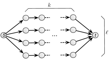
Figure 2: Graph for the proof of Theorem 1.

The functions differ only for the relatively few sets $Q$ with $|Q\cap R|>\beta$ and $|Q\setminus R|<\ell-\beta$, with $\min_{A\in\mathcal{C}}h(A)=h(C)=\ell$, $\min_{A\in\mathcal{C}}f(A)=f(R)=\beta$, where $\mathcal{C}$ is the set of cuts, and $C$ is any cut. We must have $k\ell=m$, so define $\epsilon$ such that $\epsilon^{2}=8/7\log m$, and set $k=8\sqrt{m}/\epsilon$ and $\ell=\epsilon\sqrt{m}/8$.

We compute the probability that $f$ and $h$ differ for a given query set $Q$. Probabilities are over the random unknown $R$. Since $f\leq h$, the probability of a difference is $\mathrm{Pr}(f(Q)<h(Q))$. If $|Q|\leq\ell$, then $f(Q)<h(Q)$ only if $\beta<|Q\cap R|$, and the probability $\mathrm{Pr}(f(Q)<h(Q))=\mathrm{Pr}(|Q\cap R|>\beta)$ increases as $Q$ grows. If, on the other hand, $|Q|\geq\ell$, then since $h(Q)=\ell$ the probability

$$\mathrm{Pr}(f(Q)<h(Q))=\mathrm{Pr}(|Q\setminus R|+\min\{|Q\cap R|,\;\beta\}<\ell)=\mathrm{Pr}(|Q\cap R|>\beta)$$

decreases as $Q$ grows. Hence, the probability of a difference is largest when $|Q|~{}=~{}\ell$.

So let $|Q|=\ell$. If $Q$ spreads over $b\leq k$ edges of a path $P$, then the probability that $Q$ includes the edge in $P\cap R$ is $b/k$. The expected overlap between $Q$ and $R$ is the sum of hits on all paths: $\mathbb{E}[~{}|Q\cap R|~{}]=|Q|/k=\ell/k$. Since the edges in $R$ are independent across different paths, we may bound the probability of a large intersection by a Chernoff bound (with $\delta=7$ in [56]):

$$\mathrm{Pr}\big{(}\,f(Q)\neq h(Q)\big{)}\, \leq\,\mathrm{Pr}\big{(}\,|Q\cap R|\geq 8\ell/k\;\big{)}$$ (17)

$$\leq\;2^{-7\ell/k}\;=\;2^{-7\epsilon^{2}/8}=2^{-\omega(\log m)}=m^{-\omega(1)}.$$ (18)

With this result, Lemma 1 applies. No polynomial-time algorithm can guarantee to be able to distinguish $f$ and $h$ with high probability. A polynomial algorithm with approximation factor better than the ratio of optima $h(R)/f(R)$ would discriminate the two functions and thus lead to a contradiction. As a result, the lower bound is determined by the ratio of optima of $h$ and $f$. The optimum of $f$ is $f(R)=\beta$, and $h$ has uniform cost $\ell$ for all minimal cuts. Hence, the ratio is $h(R)/f(R)=\ell/\beta=\sqrt{m}/\epsilon=o(\sqrt{m/\log m})$. ∎∎

Building on the construction in the above proof with $\ell=n^{1/3}$ and a different cut cost function, Balcan and Harvey (2012) proved that if the data structure used by an algorithm (even with an arbitrary number of queries) has polynomial size, then this data structure cannot represent the minimizers of their cooperative cut problem to an approximation factor of $o(n^{1/3}/\log n)$.

In addition, we mention that a reduction from Graph Bisection serves to prove that MinCoopCut is NP-hard. We defer the proof to Appendix C, but point out that in the reduction, the cost function is fully accessible and given as a polynomial-time computable formula.

Theorem 2.

Minimum Cooperative $(s,t)$-Cut is NP-hard.

4 Relaxation and the flow dual

As a first step towards approximation algorithms, we formulate a relaxation of MinCoopCut and analyze the flow-cut gap. The minimum cooperative cut problem can be relaxed to a continuous convex optimization problem using the convex Lovász extension $\tilde{f}$ of $f$:

$$\min_{y\in\mathbb{R}^{|\mathcal{E}|},\,x\in\mathbb{R}^{|\mathcal{V}|}}\;\; \tilde{f}(y)$$ (19)

$$\text{s.t.}\quad-x(u)+x(v)+y(e) \geq 0\quad\text{for all }e=(u,v)\in\mathcal{E}$$

$$x(s)-x(t) \geq 1$$

$$y \geq 0$$

The dual of this problem can be derived by writing the Lovász extension as a maximum $\tilde{f}(y)=\max_{z\in\mathcal{P}(f)}z^{\top}y$ of linear functions. The maximum is taken over the submodular polyhedron

$$\mathcal{P}(f)=\{y\mid\sum_{e\in A}y(e)\leq f(A)\;\forall A\subseteq\mathcal{E}\}.$$ (20)

The resulting dual problem is a flow problem with non-local capacity constraints:

$$\max_{\nu\in\mathbb{R},\varphi\in\mathbb{R}^{|\mathcal{E}|}}\quad \;\nu$$ (21)

$$\text{s.t. }\quad\;\;\varphi(A)\triangleq\sum_{e\in A}\varphi(e)\; \leq\;f(A)\;\;\;\text{ for all }A\subseteq\mathcal{E}$$ (22)

$$\sum_{e\in\delta^{+}u}\varphi(e)-\sum_{e^{\prime}\in\delta^{-}u}\varphi(e^{\prime})\; =\;d(u)\nu\quad\text{ for all }u\in\mathcal{V}$$

$$\varphi \geq 0,$$

where $d(u)=1$ if $u=s$, $d(u)=-1$ if $u=t$, and $d(u)=0$ otherwise. Constraint (22) demands that $\varphi$ must, in addition to satisfying the common flow conservation, reside within the submodular polyhedron $\mathcal{P}(f)$. This more restrictive constraint replaces the edge-wise capacity constraints that occur when $f$ is a sum of weights.

As an alternative to (19), the constraints can be stated in terms of paths: a set of edges is a cut if it intersects all $(s,t)$-paths in the graph.

$$\min\; \;\tilde{f}(y)$$ (23)

s.t. $$\sum\nolimits_{e\in P}y(e)\geq 1\;\;\;\text{for all }(s,t)\text{-paths }P\subseteq\mathcal{E}$$

$$y\in[0,1]^{\mathcal{E}}.$$

We will use this form in Section 5.2.1, and the relaxation (19) in Section 5.2.2.

4.1 Flow-cut gap

The relaxation (19) of the discrete problem (2) is not tight. This becomes evident when analyzing the ratio $f(C^{*})/\tilde{f}(y^{*})$ between the optimal value of the discrete problem and the relaxation (19) (i.e., the integrality gap). This ratio is, by strong duality between Problems (19) and (21), also the flow-cut gap $f(C^{*})/\nu^{*}$ of the optimal cut and maximal flow values.

Lemma 2.

Let $\mathcal{P}$ be the set of all $(s,t)$-paths in the graph. The flow-cut gap $f(C^{*})/\nu^{*}$ can be upper and lower bounded as follows:

$$\frac{f(C^{*})}{\sum_{P\in\mathcal{P}}\min_{P^{\prime}\subseteq P}\frac{f(P^{\prime})}{|P^{\prime}|}}\leq\frac{f(C^{*})}{\nu^{*}}\leq\frac{f(C^{*})}{\max_{P\in\mathcal{P}}\min_{P^{\prime}\subseteq P}\frac{f(P^{\prime})}{|P^{\prime}|}}.$$

Proof.

The Lemma straightforwardly follows from bounding the optimal flow $\nu^{*}$. The flow through a single path $P\in\mathcal{P}$, if all other edges $e\notin\mathcal{P}$ are empty, is restricted by the minimum average capacity for any subset of edges within the path, i.e., $\min_{P^{\prime}\subseteq P}\frac{f(P^{\prime})}{|P^{\prime}|}$. Moreover, we obtain a family of feasible solutions as those that send nonzero flow only along one path and remain within that path’s capacity. Hence, the maximum flow must be at least as big as the flow for any of those single-path solutions. This observation yields the upper bound on the ratio.

A similar argumentation shows the lower bound: the total joint capacity constraint is upper bounded by $\hat{f}(A)=\sum_{P\in\mathcal{P}}f(A\cap P)\geq f(A)$. Hence, $\sum_{P\in\mathcal{P}}\min_{P^{\prime}\subseteq P}\frac{f(P^{\prime})}{|P^{\prime}|}$ is the value of the maximum flow with capacity $\hat{f}$ if each edge is only contained in one path, and is an upper bound on the flow otherwise. ∎∎

Corollary 1.

The flow-cut gap for MinCoopCut can be as large as $n-1$.

Proof.

Corollary 1 can be shown via an example where the upper and lower bound of Lemma 2 coincide. The worst-case example for the flow-cut gap is a simple graph that consists of one single path from $s$ to $t$ with $n-1$ edges. For this graph one of the capacity constraints is that

$$\varphi(\mathcal{E})=\sum_{e\in\mathcal{E}}\varphi(e)\leq f(\mathcal{E}).$$ (24)

Constraint (24) is the only relevant capacity constraint if the capacity (and cut cost) function is $f(A)=\max_{e\in A}w(e)$ with weights $w(e)=\gamma$ for all $e\in\mathcal{E}$ and some constant $\gamma>0$ and, consequently, $f(\mathcal{E})=\gamma$. By Constraint (24), the maximum flow is $\nu^{*}=\frac{\gamma}{n-1}$. The optimum cooperative cut $C^{*}$, by contrast, consists of any single edge and has cost $f(C^{*})=\gamma$. ∎∎

Single path graphs as used in the previous proof can provide worst-case examples for rounding methods too: if $f$ is such that $f(e)\geq f(\mathcal{E})/|\mathcal{E}|$ for all edges $e$ in the path, then the solution to the relaxed cut problem is maximally uninformative: all entries of the vector $y$ are $y(e)=\frac{f(\mathcal{E})}{n-1}$.

5 Approximation algorithms

We next address approximation algorithms whereby we consider two complementary approaches. The first approach is to substitute the submodular cost function $f$ by a simpler function $\hat{f}$. Appropriate candidate functions $\hat{f}$ that admit an exact cut optimization are the approximation by Goemans et al. (2009) (Section 5.1.1), semi-gradient based approximations (Section 5.1.2), or approximations by making $f$ separable across local neighborhoods (Section 5.1.3).

The second approach is to solve the relaxations from Section 4 and round the resulting optimal fractional solution (Section 5.2.2). Conceptually very close to the relaxation approach, we offer another algorithm that solves the mathematical program (23) via a randomized greedy algorithm (Section 5.2.1).

The relaxations approaches are affected by the flow-cut gap, or, equivalently, the length of the longest path in the graph. The approximations that use a surrogate cost function are complementary and not affected by the “length”, but by a notion of the “width” of the graph.

approximating $f$		relaxation
generic (§5.1.1)	$O(\sqrt{m}\log m)$	randomized (§5.2.1)	$|P_{\max}|$
semigradient (§5.1.2)	$\frac{|C^{*}|}{(|C^{*}|-1)(1-\kappa_{f})+1}$	rounding I (§5.2.2)	$|P_{\max}|$
polymatroidal flow (§5.1.3)	$\min\{\Delta_{s},\Delta_{t}\}$	rounding II (§5.2.2)	$|\mathcal{V}|-1$

Table 2: Overview of the algorithms and their approximation factors.

5.1 Approximating the cost function

We begin with algorithms that use a suitable approximation $\hat{f}$ to $f$, for which the problem

$$\text{minimize }\hat{f}(C)\quad\text{s.t. $C\subseteq\mathcal{E}$ is a cut}$$ (25)

is solvable exactly in polynomial time. The following lemma will be the basis for the approximation bounds.

Lemma 3.

Let $\widehat{S}=\operatorname*{argmin}_{S\in\mathcal{S}}\hat{f}(S)$. If for all $S\subseteq\mathcal{E}$, it holds that $f(S)\leq\hat{f}(S)$, and if for the optimal solution $S^{*}$ to Problem (2), it holds that $\hat{f}(S^{*})\leq\alpha f(S^{*})$, then $\widehat{S}$ is an $\alpha$-approximate solution to Problem (2):

$$f(\widehat{S})\;\leq\;\alpha f(S^{*}).$$

Proof.

Since $\hat{f}(\widehat{S})\leq\hat{f}(S^{*})$, it follows that $f(\widehat{S})\leq\hat{f}(\widehat{S})\leq\hat{f}(S^{*})\leq\alpha f(S^{*})$. ∎∎

5.1.1 A generic approximation

Goemans et al. (2009) define a generic approximation of a monotone submodular function that has the functional form $\hat{f}_{ea}(A)=\sqrt{\sum_{e\in A}w_{f}(e)}$. The weights $w_{f}(e)$ depend on $f$. When using $\hat{f}_{ea}$, we compute a minimum cut for the cost $\hat{f}_{ea}^{2}$, which is a modular sum of weights and hence results in a standard Minimum $(s,t)$-Cut problem. In practice, the bottleneck lies in computing the weights $w_{f}$. Goemans et al. (2009) show how to compute weights such that $f(A)\leq\hat{f}(A)\leq\alpha f(A)$ with $\alpha=O(\sqrt{m})$ for a matroid rank function, and $\alpha=O(\sqrt{m}\log m)$ otherwise. We add that for an integer polymatroid rank function bounded by $M=\max_{e\in\mathcal{E}}f(e)$, the logarithmic factor can be replaced by a constant to yield $\alpha=O(\sqrt{mM})$ (if one approximates the matroid expansion of the polymatroid instead of $f$ directly). Together with Lemma 3, this yields the following approximation bounds.

Lemma 4.

Let $\widehat{C}=\operatorname*{argmin}_{C\in\mathcal{C}}\hat{f}_{ea}(C)$ be the minimum cut for cost $\hat{f}_{ea}$, and $C^{*}=\operatorname*{argmin}_{C\in\mathcal{C}}f(C)$. Then $f(\widehat{C})=O(\sqrt{m}\log m)f(C^{*})$. If $f$ is integer-valued and we approximate its matroid expansion, then $f(\widehat{C})=O(\sqrt{mM})f(C^{*})$, where $M\leq\max_{e}f(e)$.

The lower bound in Theorem 1 suggests that for sparse graphs, the bound in Lemma 4 is tight up to logarithmic factors.

5.1.2 Approximations via semigradients

For any monotone submodular function $f$ and any set $A$, there is a simple way to compute a modular upper bound $\hat{f}_{s}$ to $f$ that agrees with $f$ at $A$. In other words, $\hat{f}_{s}$ is a discrete supergradient of $f$ at $A$. We define $\hat{f}_{s}$ as (Jegelka and Bilmes, 2011a; Iyer et al., 2013a)

$$\hat{f}_{s}(B;A)=f(A)+\sum_{e\in B\setminus A}f(e\mid A)-\sum_{e\in A\setminus B}f(e\mid\mathcal{E}\setminus e).$$ (26)

Lemma 5.

Let $\widehat{C}\in\operatorname*{argmin}_{C\in\mathcal{C}}\hat{f}_{s}(C;\emptyset)$. Then

$$f(\widehat{C})\leq\frac{|C^{*}|}{(|C^{*}|-1)(1-\kappa_{f})+1}f(C^{*}),$$

where $\kappa_{f}=\max_{e}\,\big{(}1-\frac{f(e\mid\mathcal{E}\setminus e)}{f(e)}\big{)}$ is the curvature of $f$.

Lemma 5 was shown in (Iyer et al., 2013a). As $m$ (and correspondingly $|C^{*}|$) gets large, the bound eventually no longer depends on $m$ and instead only on the curvature of $f$. In practice, results are best when the supergradient is used in an iterative algorithm: starting with $C_{0}=\emptyset$, one computes $C_{t}\in\operatorname*{argmin}_{C\in\mathcal{C}}\hat{f}_{s}(C;C_{t-1})$ until the solution no longer changes between iterations. The minimum cut for the cost function $\hat{f}_{s}(C;A)$ can be computed as a minimum cut with edge weights

$$w(e)=\begin{cases}f(e\mid\mathcal{E}\setminus e)&\text{ if }e\in A\\ f(e\mid A)&\text{ if }e\notin A.\end{cases}$$ (27)

Consequently, the semigradient approximation yields a very easy and practical algorithm that iteratively uses standard minimum cut as a subroutine. This algorithm was used e.g. in (Jegelka and Bilmes, 2011a), and the visual results in (Kohli et al., 2013) show that it typically yields very good solutions in practice on certain problem instances where the optimum solution can be computed exactly.

5.1.3 Approximations by introducing separation

The approximations in Section 5.1.1 and 5.1.2 are indifferent to the structure of the graph, while following approximation is not. One may say that Problem (2) is hard because $f$ introduces non-local dependencies between edges that might be anywhere in the graph. Indeed, the problem is easier if dependencies between edges are restricted to local neighborhoods defined by the graph, for example, edges that might be incident to the same vertex.

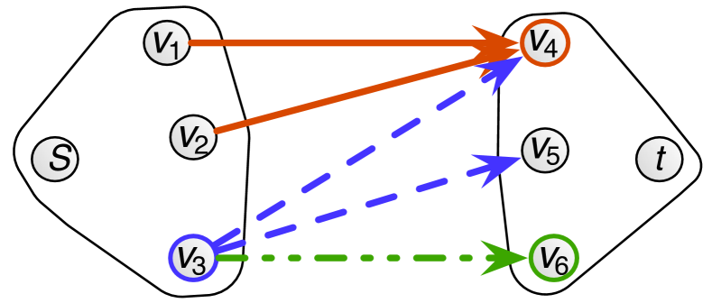
$$\hat{f}_{pf}(C)= f(\{(v_{1},v_{4}),(v_{2},v_{4})\})$$

$$+f(\{(v_{3},v_{4}),(v_{3},v_{5})\})$$

$$+f(\{(v_{3},v_{6})\})$$

Figure 3: Approximation of a cut cost. Red edges are in $C^{\Pi}_{v_{4}}$ (head), blue dashed edges in $C^{\Pi}_{v_{3}}$ (tail), and the green dash-dotted edge in $C^{\Pi}_{v_{6}}$ (head).

Hence, we define an approximation $\hat{f}_{pf}$ that is globally separable but locally exact. To measure the cost of an edge set $C\subseteq\mathcal{E}$, we partition $C$ into groups $\Pi(C)=\{C^{\Pi}_{v}\}_{v\in V}$, where the edges in set $C^{\Pi}_{v}$ must be incident to node $v$ ($C_{v}^{\Pi}$ may be empty). That is, we assign each edge either to its head or to its tail node in any partition, as illustrated in Figure 3. Let $\mathcal{P}_{C}$ be the family of all such partitions (which vary over the head or tail assignment of each edge). We define an approximation

$$\hat{f}_{pf}(C)=\min_{\Pi(C)\in\mathcal{P}_{C}}\sum\nolimits_{v\in V}f(C^{\Pi}_{v})$$ (28)

that (once the partition is fixed) decomposes across different node incidence edge sets, but is accurate within a group $C^{\Pi}_{v}$. Thanks to the subadditivity of $f$, the function $\hat{f}_{pf}$ is an upper bound on $f$. It is a convolution of submodular functions and always is the tightest approximation that is a direct sum over any partition in $\mathcal{P}_{C}$. Perhaps surprisingly, even though the approximation (28) looks difficult to compute and is in general not even a submodular function (an example is in Appendix D), it is possible to solve a minimum cut with cost $\hat{f}_{pf}$ exactly. To do so, we exploit its duality to a generalized maximum flow problem, namely polymatroidal network flows.

Polymatroidal network flows.

Polymatroidal network flows (Lawler and Martel, 1982; Hassin, 1982) generalize the capacity constraint of traditional flow problems. They retain the constraint of flow conservation (a function $\varphi:\mathcal{E}\to\mathbb{R}_{+}$ is a flow if the inflow at each node $v\in\mathcal{V}\setminus\{s,t\}$ equals the outflow). The edge-wise capacity constraint $\varphi(e)\leq\mathrm{cap}(e)$ for all $e\in\mathcal{E}$, given a capacity function $\mathrm{cap}:\mathcal{E}\to\mathbb{R}_{+}$ is replaced by local submodular capacities over sets of edges incident at each node $v$: $\mathrm{cap}_{v}^{\text{in}}$ for incoming edges, and $\mathrm{cap}_{v}^{\text{out}}$ for outgoing edges. The capacity constraints at each $v\in\mathcal{V}$ are

$$\varphi(A) \leq\mathrm{cap}_{v}^{\text{in}}(A)\quad\;\,\text{ for all }A\subseteq\delta^{-}(v)\;\text{(incoming edges), and}$$

$$\varphi(A) \leq\mathrm{cap}_{v}^{\text{out}}(A)\quad\text{ for all }A\subseteq\delta^{+}(v)\;\text{(outgoing edges)}.$$

Each edge $(u,v)$ belongs to two incidence sets, $\delta^{+}u$ and $\delta^{-}v$. A maximum flow with such constraints can be found in time $O(m^{4}\tau)$ by the layered augmenting path algorithm by Tardos et al. (1986), where $\tau$ is the time to minimize a submodular function on any set $\delta^{+}v$, $\delta^{-}v$ for any $v$. Hence, the incidence sets are in general much smaller than $\mathcal{E}$.

A special polymatroidal maximum flow turns out to be dual to the cut problem we are interested in. To see this, we will use the restriction $\mathchoice{{f\,\smash{\vrule height=5.55557pt,depth=1.65279pt}}_{\,A}}{{f\,\smash{\vrule height=5.55557pt,depth=1.65279pt}}_{\,A}}{{f\,\smash{\vrule height=3.88889pt,depth=1.16167pt}}_{\,A}}{{f\,\smash{\vrule height=2.77777pt,depth=1.16167pt}}_{\,A}}$ of the function $f$ to a subset $A$. For ease of reading we drop the explicit restriction notation later. We assume throughout that the desired cut is minimal, since additional edges can only increase its cost.

Lemma 6.

Minimum $(s,t)$-cut with cost function $\hat{f}_{pf}$ is dual to a polymatroidal network flow with capacities $\mathrm{cap}_{v}^{\text{in}}=\mathchoice{{f\,\smash{\vrule height=5.55557pt,depth=1.94556pt}}_{\,\delta^{-}v}}{{f\,\smash{\vrule height=5.55557pt,depth=1.94556pt}}_{\,\delta^{-}v}}{{f\,\smash{\vrule height=3.88889pt,depth=1.47334pt}}_{\,\delta^{-}v}}{{f\,\smash{\vrule height=2.77777pt,depth=1.47334pt}}_{\,\delta^{-}v}}$ and $\mathrm{cap}_{v}^{\text{out}}=\mathchoice{{f\,\smash{\vrule height=5.55557pt,depth=2.04944pt}}_{\,\delta^{+}v}}{{f\,\smash{\vrule height=5.55557pt,depth=2.04944pt}}_{\,\delta^{+}v}}{{f\,\smash{\vrule height=3.88889pt,depth=1.57721pt}}_{\,\delta^{+}v}}{{f\,\smash{\vrule height=2.77777pt,depth=1.57721pt}}_{\,\delta^{+}v}}$ at each node $v\in\mathcal{V}$.

The proof is provided in Appendix E. It uses, with some additional considerations, the dual problem to a polymatroidal maxflow, which can be stated as follows. Let $\mathrm{cap}^{\text{in}}:2^{\mathcal{E}}\to\mathbb{R}_{+}$ be the joint incoming capacity function, i.e., $\mathrm{cap}^{\text{in}}(C)=\sum_{v\in V}\mathrm{cap}_{v}^{\text{in}}(C\cap\delta^{-}v)$, and let equivalently $\mathrm{cap}^{\text{out}}$ be the corresponding joint outgoing capacity. The dual of the polymatroidal maximum flow is a minimum cut problem whose cost is a convolution of edge capacities (Lovász, 1983):

$$\mathrm{cap}(C)=(\mathrm{cap}^{\text{in}}\ast\mathrm{cap}^{\text{out}})(C)\;\triangleq\;\min_{A\subseteq C}\Bigl{[}\mathrm{cap}^{\text{in}}(A)+\mathrm{cap}^{\text{out}}(C\setminus A)\Bigr{]}.$$ (29)

This convolution is in general not a submodular function. Lemma 6 implies that we can solve the approximate MinCoopCut via its dual flow problem. The primal cut solution will be given by a set of full edges, i.e., edges whose joint flow equals their joint capacity.

We can now state the resulting approximation bound for MinCoopCut. Let $C^{*}$ be the optimal cut for cost $f$. We define $\Delta_{s}$ to be the tail nodes of the edges in $C^{*}$: $\Delta_{s}=\{v\mid\exists(v,u)\in C^{*}\}$, and similarly, $\Delta_{t}=\{v\mid\exists(u,v)\in C^{*}\}$. The sets $\Delta_{s},\Delta_{t}$ provide a measure of the “width” of the graph.

Theorem 3.

Let $\widehat{C}$ be the minimum cut for cost $\hat{f}_{pf}$, and $C^{*}$ the optimal cut for cost $f$. Then

$$f(\widehat{C})\;\leq\;\min\{|\Delta_{s}|,|\Delta_{t}|\}\,f(C^{*})\;\leq\;\frac{|\mathcal{V}|}{2}f(C^{*}).$$

Proof.

To apply Lemma 3, we need to show that $f(C)\leq\hat{f}_{pf}(C)$ for all $C\subseteq\mathcal{E}$, and find an $\alpha$ such that $\hat{f}_{pf}(C^{*})\leq\alpha f(C^{*})$. The first condition follows from the subadditivity of $f$.

To bound $\alpha$, we use Lemma 6 and Equation 29:

$$\hat{f}_{pf}(C^{*}) =(\mathrm{cap}^{\text{in}}\ast\mathrm{cap}^{\text{out}})(C^{*})$$ (30)

$$\leq\min\{\mathrm{cap}^{\text{in}}(C^{*}),\;\mathrm{cap}^{\text{out}}(C^{*})\}$$ (31)

$$\leq\min\Big{\{}\sum\nolimits_{v\in\Delta_{s}}f(C^{*}\cap\delta^{+}v),\;\;\sum\nolimits_{v\in\Delta_{t}}f(C^{*}\cap\delta^{-}v)\Big{\}}$$ (32)

$$\leq\min\Big{\{}|\Delta_{s}|\max_{v\in\Delta_{s}}f(C^{*}\cap\delta^{+}v),\;\;|\Delta_{t}|\max_{v\in\Delta_{t}}f(C^{*}\cap\delta^{-}v)\Big{\}}$$ (33)

$$\leq\min\big{\{}\,|\Delta_{s}|,\;|\Delta_{t}|\,\big{\}}\;f(C^{*}).$$ (34)

Thus, Lemma 3 implies an approximation bound $\alpha\leq\min\big{\{}\,|\Delta_{s}|,\;|\Delta_{t}|\,\big{\}}\leq|\mathcal{V}|/2$. ∎∎

Iyer et al. (2013b) show that the bound in Theorem 3 can be tightened to $\frac{|\mathcal{V}|}{2+(|\mathcal{V}|-2)(1-\kappa_{f})}$ by taking into account the curvature $\kappa_{f}$ of $f$.

5.2 Relaxations

An alternative approach to approximating the edge weight function $f$ is to relax the cut constraints via the formulations (23) and (19). We analyze two algorithms: the first, a randomized algorithm, maintains a discrete solution, while the second is a simple rounding method. Both cases remove the constraint that the cut must be minimal: any set $B$ is feasible that has a subset $C\subseteq B$ that is a cut. Relaxing the minimality constraint makes the feasible set up-monotone (equivalently up-closed). This is not major problem, however, since any superset of a cut can easily be pruned to a minimal cut while only, if anything, improving the solution due to the monotonicity of $f$.

5.2.1 Randomized greedy covering

The constraints in the path-based relaxation (23) suggest that a minimum $(s,t)$-cut problem is also a min-cost cover problem: a cut must intersect or “cover” each $(s,t)$-path in the graph. The covering formulation of the constraints in (23) clearly show the relaxation of the minimality constraint. Algorithm 1 solves a discrete variant of the formulation (23) and maintains a discrete $y\in\{0,1\}$, i.e., $y$ is eventually the indicator vector of a cut.

Since a graph can have exponentially many $(s,t)$-paths, there can be exponentially many constraints. But all that is needed in the algorithm is to find a violated constraint, and this is possible by computing the shortest path $P_{\min}$, using $y$ as the (additive) edge lengths. If $P_{\min}$’s weight is at least one, then $y$ is feasible. Otherwise, $P_{\min}$ defines a violated constraint in formulation (23).

  Input: graph $\mathcal{G}=(\mathcal{V},\mathcal{E})$, terminal nodes $s,t\in\mathcal{V}$, cost function $f:2^{\mathcal{E}}\to\mathbb{R}_{+}$

  $C=\emptyset$, $y=0$

  while $\sum_{e\in P_{\min}}y(e)<1$ for the current shortest path $P_{\min}$ do

     choose $\beta$ within the interval $\beta\in(0,\min_{e\in P_{\min}}f(e|C)]$

     for $e$ in $P_{\min}$ do

        with probability $\beta/f(e|C)$, set $C=C\cup\{e\}$, $y(e)=1$.

     end for

  end while

  prune $C$ to $C^{\prime}$ and return $C^{\prime}$

Algorithm 1 Greedy randomized path cover

Owing to the form of the constraints, we can adapt a randomized greedy cover algorithm (Koufogiannakis and Young, 2009) to Problem (23) and obtain Algorithm 1. In each step, we compute the shortest path with weights $y$ to find a possibly uncovered path. Ties are resolved arbitrarily. To cover the path, we randomly pick edges from $P_{\min}$. The probability of picking edge $e$ is inversely proportional to the marginal cost $f(e|C)$ of adding $e$ to the current selection of edges. We must also specify an appropriate $\beta$. With the maximal allowed $\beta=\min_{e\in P_{\min}}f(e|C)$, the cheapest edges are selected deterministically, and others randomly. In that case, $C$ grows by at least one edge in each iteration, and the algorithm terminates after at most $m$ iterations.

If the algorithm returns a set $C$ that is feasible but not a minimal cut, it is easy to prune it to a minimal cut $C^{\prime}\subseteq C$ without any additional approximation error, since monotonicity of $f$ implies that $f(C^{\prime})\leq f(C)$. Such pruning can for example be done via breadth-first search. Let $\mathcal{V}_{s}$ be the set of nodes reachable from $s$ after the edges in $C$ have been removed. Then we set $C^{\prime}=\delta^{+}(\mathcal{V}_{s})$. The set $C^{\prime}$ must be a subset of $C$, since if there was an edge $(u,v)\in C^{\prime}\setminus C$, then $v$ would also be in $\mathcal{V}_{s}$, and then $(u,v)$ cannot be in $C^{\prime}$, a contradiction.

The approximation bound for Algorithm 1 is the length of the longest path, like that of the rounding methods in Section 5.2.2. This is not a coincidence, since both algorithms essentially use the same relaxation.

Lemma 7.

In expectation (over the probability of sampling edges), Algorithm 1 returns a solution $\widehat{C}^{\prime}$ with $\mathbb{E}[f(\widehat{C}^{\prime})]\leq|P_{\max}|f(C^{*})$, where $P_{\max}$ is the longest simple $(s,t)$-path in $\mathcal{G}$.

Proof.

Let $\widehat{C}$ be the cut before pruning. Since $f$ is nondecreasing, it holds that $f(\widehat{C}^{\prime})\leq f(\widehat{C})$. By Theorem 7 in (Koufogiannakis and Young, 2009), a greedy randomized procedure like Algorithm 1 yields in expectation an $\alpha$-approximation for a cover, where $\alpha$ is the maximum number of variables in any constraint. Here, $\alpha$ is the maximum number of edges in any simple path, i.e., the length of the longest path. This implies that $\mathbb{E}[f(\widehat{C}^{\prime})]\leq\mathbb{E}[f(\widehat{C})]\leq|P_{\max}|f(C^{*})$. ∎∎

Indeed, randomization is important. Consider a deterministic algorithm that always picks the edge with minimum marginal cost in the next path to cover. The solution $\widehat{C}_{d}$ returned by this algorithm can be much worse. As an example, consider a graph consisting of a clique $\mathcal{V}$ of $n$ nodes, with nodes $s$ and $t$. Let $S\subseteq\mathcal{V}$ be a set of size $n/2$. Node $s$ is connected to all nodes in $S$, and node $t$ is connected to the clique only by a distinct node $v^{\prime}\in\mathcal{V}\setminus S$ via edge $(v^{\prime},t)$. Let the cost function be a sum of edge weights, $f(C)=\sum_{e\in C}w(e)$. Edge $(v^{\prime},t)$ has weight $\gamma>0$, all edges in $\delta^{+}(S)$ have weight $\gamma(1-\epsilon)$ for a small $\epsilon>0$, and all remaining edges have weight $\gamma(1-\epsilon/2)$. The deterministic algorithm will return $\widehat{C}_{d}=\delta^{+}(S)$ as the solution, with cost $\frac{n^{2}\gamma}{4}(1-\epsilon)$, which is by a factor of $|\widehat{C}_{d}|(1-\epsilon)=\frac{n^{2}}{4}(1-\epsilon)$ worse than the optimal cut, $f(\{(v^{\prime},t)\})=\gamma$. Hence, for the deterministic variant of Algorithm 1, we can only show the following approximation bound:

Lemma 8.

For the solution $\widehat{C}_{d}$ returned by the greedy deterministic heuristic, it holds that $f(\widehat{C}_{d})\leq|\widehat{C}_{d}|f(C^{*})$. This approximation factor cannot be improved in general.

Proof.

To each edge $e\in\widehat{C}_{d}$ assign the path $P(e)$ which it was chosen to cover. By the nature of the algorithm, it must hold that $f(e)\leq f(C^{*}\cap P(e))$, because otherwise an edge in $C^{*}\cap P(e)$ would have been chosen. Since $C^{*}$ is a cut, the set $C^{*}\cap P(e)$ must be non-empty. These observations imply that

$$f(\widehat{C}_{d})\,\leq\,\sum_{e\in\widehat{C}}f(e)\,\leq\,\sum_{e\in\widehat{C}_{d}}f(C^{*}\cap P(e))\,\leq\,|\widehat{C}_{d}|\max_{e\in\widehat{C}_{d}}f(C^{*}\cap P(e))\,\leq\,|\widehat{C}_{d}|f(C^{*}).$$

Tightness follows from the worst-case example described above. ∎∎

5.2.2 Rounding

Our last approach is to solve the convex program (19) and round the continuous to a discrete solution. We describe two types of rounding, each of which achieves a worst-case approximation factor of $n-1$. This factor equals the general flow-cut gap in Lemma 1. Let $x^{*},y^{*}$ be the optimal solution to the relaxation (19) (equivalently, to (23)). We assume w.l.o.g. that $x^{*}\in[0,1]^{n}$, $y^{*}\in[0,1]^{m}$.

Rounding by thresholding edge lengths.

The first technique uses the edge weights $y^{*}$. We pick a threshold $\theta$ and include all edges $e$ whose entry $y^{*}(e)$ is larger than $\theta$. Algorithm 2 shows how to select $\theta$, namely the largest edge length that when treated as a threshold yields a cut.

Algorithm 2 Rounding procedure given $y^{*}$

  order $\mathcal{E}$ such that $y^{*}(e_{1})\geq y^{*}(e_{2})\geq\ldots\geq y^{*}(e_{m})$

  for $i=1,\ldots,m$ do

     let $C_{i}=\{e_{j}\;|\;y^{*}(e_{j})\geq y^{*}(e_{i})\}$

     if $C_{i}$ is a cut then

        prune $C_{i}$ to $\widehat{C}$ and return $\widehat{C}$

     end if

  end for

Lemma 9.

Let $\widehat{C}$ be the rounded solution returned by Algorithm 2, $\theta$ the threshold at the last iteration $i$, and $C^{*}$ the optimal cut. Then

$$f(\widehat{C})\;\leq\;\frac{1}{\theta}f(C^{*})\;\leq\;|P_{\max}|f(C^{*})\;\leq\;(n-1)f(C^{*}),$$

where $P_{\max}$ is the longest simple path in the graph.

Proof.

The proof is analogous to that for covering problems (Iwata and Nagano, 2009). In the worst case, $y^{*}$ is uniformly distributed along the longest path, i.e., $y^{*}(e)=|P_{\max}|^{-1}$ for all $e\in P_{\max}$ as $y^{*}$ must sum to at least one along each path. Then $\theta$ must be at least $|P_{\max}|^{-1}$ to include at least one of the edges in $P_{\max}$. Since $\tilde{f}$ is nondecreasing like $f$ and also positively homogeneous, it holds that

$$f(\widehat{C})\leq f(C_{i})=\tilde{f}(\chi_{C_{i}})\;\leq\tilde{f}(\theta^{-1}y^{*})=\theta^{-1}\tilde{f}(y^{*})\leq\theta^{-1}\tilde{f}(\chi_{C^{*}})=\theta^{-1}f(C^{*}).$$

The first inequality follows from monotonicity of $f$ and the fact that $\widehat{C}\subseteq C_{i}$. Similarly, the relation between $\tilde{f}(\chi_{C_{i}})$ and $\tilde{f}(\theta^{-1}y^{*})$ holds because $\tilde{f}$ is nondecreasing: by construction, $y^{*}(e)\geq\theta\chi_{C_{i}}(e)$ for all $e\in\mathcal{E}$, and hence $\chi_{C_{i}}(e)\leq\theta^{-1}y^{*}(e)$. Finally, we use the optimality of $y^{*}$ to relate the cost to $f(C^{*})$; the vector $\chi_{C^{*}}$ is also feasible, but $y^{*}$ optimal. The lemma follows since $\theta^{-1}\leq|P_{\max}|$. ∎∎

Rounding by node distances.

Alternatively, we can use $x^{*}$ to obtain a discrete solution. We pick a threshold $\theta$ uniformly at random from $[0,1]$ (or find the best one), and choose all nodes $u$ with $x^{*}(u)\geq\theta$ (call this $\mathcal{V}_{\theta}$). This induces the cut $C_{\theta}=\delta(\mathcal{V}_{\theta})$. Since the node labels $x^{*}$ can also be considered as distances from $s$, we refer to this rounding methods as distance rounding.

Lemma 10.

The worst-case approximation factor for a solution $C_{\theta}$ obtained with distance rounding is $\mathbb{E}_{\theta}[f(C_{\theta})]\leq(n-1)\tilde{f}(y^{*})\leq(n-1)f(C^{*})$.

Proof.

To upper bound the quantity $\mathbb{E}_{\theta}[f(C_{\theta})]$, we partition the set of edges into $(n-1)$ sets $\delta^{+}(v)$, that is, each set corresponds to the outgoing edges of a node $v\in\mathcal{V}$. We sort the edges in each $\delta^{+}(v)$ in nondecreasing order by their values $y^{*}(e)$. Consider one specific incidence set $\delta^{+}(u)$ with edges $e_{u,1},\ldots,e_{u,h}$ and $y^{*}(e_{u,1})\leq y^{*}(e_{u,2})\leq\ldots\leq y^{*}(e_{u,h})$. Edge $e_{u,i}$ is in the cut if $\theta\in[x^{*}(u),x^{*}(u)+y^{*}(e_{u,i}))$. Therefore, it holds for each node $u$ that

$$\mathbb{E}_{\theta}[f(C_{\theta}\cap\delta^{+}(u))] =\int_{0}^{1}f(C_{\theta}\cap\delta^{+}(u))d\theta$$ (35)

$$=\sum_{j=1}^{h}(y^{*}(e_{u,j})-y^{*}(e_{u,j-1}))f(\{e_{u,j},\ldots e_{u,h}\})$$ (36)

$$=\tilde{f}(y^{*}({\delta^{+}(u)})),$$ (37)

where we define $y^{*}(e_{u,0})=0$ for convenience, and assume that $f(\emptyset)=0$. This implies that

$$\mathbb{E}_{\theta}[f(C_{\theta})] \leq\mathbb{E}_{\theta}[\sum_{v\in\mathcal{V}}f(C_{\theta}\cap\delta^{+}(v))]$$ (38)

$$=\sum_{v\in\mathcal{V}}\tilde{f}(y^{*}({\delta^{+}(v)}))\leq(n-1)\tilde{f}(y^{*})\leq(n-1)f(C^{*}).$$ (39)

∎∎

A more precise approximation factor is $\frac{\sum_{v}\tilde{f}(y^{*}({\delta^{+}(v)}))}{f(y^{*})}$.

6 Special cases

The complexity of MinCoopCut is not always as bad as the worst-case bound in Theorem 1. While it is useful to consider this most general case (see Section 2.3), we next discuss properties of the submodular cost function and the graph structure that lead to better approximation factors. Our discussion is not specific to cooperative cuts; it is rather a survey of properties that make a number of submodular optimization problems easier.

6.1 Separability and sums with bounded support

An important factor for tractability and approximations is the separability of the cost function, that is, whether there are separators of $f$ whose structure aligns with the graph.

Definition 1 (Separator of $f$).

A set $S\subseteq\mathcal{E}$ is called a separator of $f:2^{\mathcal{E}}\to\mathbb{R}$ if for all $B\subseteq\mathcal{E}$, it holds that $f(B)=f(B\cap S)+f(B\setminus S)$. The set of separators of $f$ is closed under union and intersection.

The structure of the separators strongly affects the complexity of MinCoopCut. First and obviously, the extreme case that $f$ is a modular function (and each $e\in\mathcal{E}$ is a separator) can be solved exactly. Second, if the separators of $f$ form a partition $\mathcal{E}=\bigcup_{v}E^{+}_{v}\cup\bigcup_{v}E^{-}_{v}$ that aligns with node neighborhoods such that $E_{v}^{+}\subseteq\delta^{+}(v)$, and $E_{v}^{-}\subseteq\delta^{-}(v)$, then both $\hat{f}_{pf}$ and distance rounding solve the problem exactly. No change in the algorithm is needed, i.e., the exact partition need not be known. In that case, the flow-cut gap is zero, as becomes obvious from the proof of Lemma 10, since $(\sum_{v}\tilde{f}(y^{*}_{E_{v}}))/\tilde{f}(y^{*})=1$. These separators respect the graph structure and rule out any non-local edge interactions.

Sums of functions with bounded support.

A generalization of the case of separators are functions that are a sum $f(A)=\sum_{i}f_{i}(A\cap B_{i})$ of functions $f_{i}$, each of which has bounded support $B_{i}$. The $B_{i}$ can be overlapping. In this case, the approximation bounds improve for many of the algorithms in Section 5.1 that rely on a surrogate function, and for the greedy approximation in Lemma 8. Those bounds, summarized in Table 3, can be shown by approximating each $f_{i}$ separately by $\hat{f}_{i}$ with approximation factor $\alpha_{i}$ that now depends on $|B_{i}|$, and using $f(A)\leq\max_{j}\alpha_{j}\sum_{i}\hat{f}_{i}(A)$. This separate approximation is implicit in all those algorithms except the approximation from Section 5.1.1. In those implicit cases, no changes need to be made in the implementation and the partition need not be known. For the generic approximation in Section 5.1.1, one can approximate each $f_{i}$ explicitly and separately, if the partition is known. Optimizing the resulting sum $\sum_{i}\hat{f}_{i}$ or its square is however no longer a minimum cut problem. It admits an FPTAS (Nikolova, 2010; Kohli et al., 2013).

generic (§5.1.1)	$O(\max_{i}\,\sqrt{|B_{i}|}\log|B_{i}|)$
semigradient (§5.1.2)	$\max_{i}\frac{|C^{*}\cap B_{i}|}{(|C^{*}\cap B_{i}|-1)(1-\kappa_{f_{i}})+1}$
polymatroidal flow (§5.1.3)	$\max_{i}\min\{\Delta_{s}\cap B_{i},\Delta_{t}\cap B_{i}\}$
deterministic greedy (§5.2.1)	$\max_{i}|\widehat{C}_{d}\cap B_{i}|$

Table 3: Improved approximation bounds for functions of the form $f(A)=\sum_{i=1}^{k}f_{i}(A\cap B_{i})$. The bounds are now determined by the largest support $\max_{i}|B_{i}|$, but not by $k$.

For the relaxations, it is not immediately clear that the decomposition always leads to improvements. Consider for example a function $f(A)=f_{1}(A\cap B_{1})+f_{2}(A\cap B_{2})$, where $f_{1}(B_{1})=f_{2}(B_{2})$, $P\triangleq P_{\max}=B_{1}\cup B_{2}$ and $|B_{1}|=|B_{2}|=|P_{\max}/2|$. Then $\tilde{f}(\frac{1}{|P|}\chi_{P})=\tilde{f}(\frac{1}{|B_{1}|}\chi_{B_{1}})$. In that case, the proof of Lemma 9 may still require $\theta^{-1}=|P_{\max}|$.

6.2 Symmetry and “unstructured” functions

Going one step further, one may consider sums of that do not necessarily have bounded support but are of a simpler form. An important such class are functions $f_{i}(A)=g(\sum_{e\in A}w_{i}(e))=g(w_{i}(A))$ for nonnegative weights $w_{i}(e)$ and a nondecreasing concave function $g$. We refer to the submodular functions $g(w(A))$ as unstructured, because they only consider a sum of weights, but otherwise do not make any distinction between edges (unlike, e.g., graphic matroid rank functions). One may classify such functions into a hierarchy, where $\mathcal{F}(k)$ contains all functions $f(A)=\sum_{j=1}^{k}g_{j}(w_{j}(A))$ with at most $k$ such components. The functions $\mathcal{F}(k)$ are special cases of low-rank quasi-concave functions, where $k$ is the rank of the function.

If $k=1$, then it suffices to minimize $w_{1}(C)$ directly and the problem reduces to Minimum $(s,t)$-Cut. For $k>1$, several combinatorial problems admit an FPTAS with running time exponential in $k$ (Goyal and Ravi, 2008; Mittal and Schulz, 2012). This holds for cooperative cuts too (Kohli et al., 2013). A special case for $k=2$ is the mean-risk objective $f(A)=w_{1}(A)+\sqrt{w_{2}(A)}$ (Nikolova, 2010). Goel et al. (2010) show that these functions can yield better bounds in combinatorial multi-agent problems than general polymatroid rank functions, if each agent has a cost function in $\mathcal{F}(1)$.

Even for general, unconstrained submodular minimization, the class $\mathcal{F}(k)$ admits specialized improved optimization algorithms (Kohli et al., 2009a; Stobbe and Krause, 2010; Kolmogorov, 2012; Jegelka et al., 2013). The complexity of those faster specialized algorithms depends on the rank $k$ as well. An interesting question arising from the above observations is whether $\mathcal{F}(k)$ contains all submodular functions if $k$ is large enough? The answer is no: even if $k$ is allowed to be exponentially large in the ground set size, this class is a strict sub-class of all submodular functions. If the addition of auxiliary variables is allowed, this class coincides with the class of graph-representable functions in the sense of (Z̆ivný et al., 2009): any graph cut function $h:2^{\mathcal{V}}\to\mathbb{R}_{+}$ is in $\mathcal{F}(|\mathcal{E}|)$, and any function in $\mathcal{F}(k)$ can be represented as a graph cut function in an extended auxiliary graph (Jegelka et al., 2011). However, not all submodular functions can be represented in this way (Z̆ivný et al., 2009).

The parameter $k$ is a measure of complexity. If $k$ is not fixed, then MinCoopCut is NP-hard; for example, the reduction in Section C uses such functions. Even more, unrestricted $k$ may induce large lower bounds, as has been proved for label cost functions of the form $f(A)=\sum_{j=1}^{k}w_{j}\min\{1,|A\cap B_{j}|\}$ (Zhang et al., 2011).

A subclass of unstructured submodular functions are the aforementioned permutation symmetric submodular functions that are indifferent to any permutation of the ground set: $f(A)=f(\sigma(A))$ for all permutations $\sigma$ (possibly within a group). This symmetry makes submodular optimization problems easier, as shown in Proposition 3 and work on submodular maximization (Vondrák, 2013) and partitioning problems (Ene et al., 2013).

6.3 Symmetry and graph structure

Proposition 3 shows that symmetry and the graph structure can work together to make the cut problem easier, in fact, a submodular minimization problem on graph nodes. Section 2 outlines some examples that come from applications.

6.4 Curvature

The curvature $\kappa_{f}\in[0,1]$ of a submodular function $f$ is defined as

$$\kappa_{f}=\max_{e\in\mathcal{E}}\;\;1-\frac{f(e\mid\mathcal{E}\setminus e)}{f(e)},$$ (40)

and characterizes the deviation from being a modular function. Curvature is known to affect the approximation bounds for submodular maximization (Conforti and Cornuéjols, 1984; Vondrák, 2008), and also for submodular minimization problems, approximating and learning submodular functions (Iyer et al., 2013b). The lower the curvature, the better the approximation factors. For MinCoopCut and many other combinatorial minimization problems with submodular costs, the approximation factor is affected as follows. If $\alpha_{n}$ is the worst-case factor (e.g., for the semigradient approximation), then the tightened factor is $\frac{\alpha_{n}}{(\alpha_{n}-1)(1-\kappa_{f})+1}$. The lower bounds can be tightened accordingly.

6.5 Flow-cut gaps revisited

The above properties that facilitate MinCoopCut reduce the flow-cut gaps in some cases. The proof of Lemma 1 illustrates that the flow-cut gap is intricately linked to the edge cooperation (non-separability) along paths in the graph. Therefore, the separability described in Section 6.1 affects the flow-cut gap if it breaks up cooperation along paths: the gap depends only on the longest cooperating path within any separator of $f$, and this can be much smaller than $n$. If, however, an instance of MinCoopCut is better solvable because the cost function is a member of $\mathcal{F}(\ell)$ for small constant $\ell$, then the gap may still be as large as in Lemma 1. In fact, the example in Lemma 1 belongs to $\mathcal{F}(1)$: it is equivalent to the function $f(A)=\gamma\min\{1,|A|\}$.

Two variants of a final example may serve to better understand the flow-cut (and integrality) gap. The first has a large gap, but the rounding methods still find an optimal solution. The second has a gap of one, but the rounding methods may return solutions with a large approximation factor. Consider a graph with $m$ edges consisting of $m/k$ disjoint paths of length $k$ each (as in Figure 2), with a cost function $f(C)=\max_{e\in C}w(e)$. The edges are partitioned into a cut $B\subset\mathcal{E}$ with $|B|=m/k$ and the remaining edges $\mathcal{E}\setminus B$. Let $w(e)=\gamma$ for $e\notin B$ and $w(e)=\beta$ for $e\in B$.

For the first variant, let $\beta=\gamma$; so that for $k=1$, we obtain the graph in Lemma 1. With $\beta=\gamma$ (for any $k$), any minimal cut is optimal, and all rounding methods find an optimal solution. The maximum flow in Problem (21) is $\nu^{*}=\gamma/k$ ($\gamma/k$ flow on one path or $\gamma/m$ flow on each edge in $m/k$ paths in parallel). Hence, the flow-cut gap is $\gamma/(\gamma/k)=k$ despite the optimality of the rounded (and pruned) solutions.

For the second variant, let $\beta=\gamma/k$. The maximum flow remains $\nu^{*}=\gamma/k$, and the optimal cut is $B$ with $f(B)=\gamma/k$, so $f(C^{*})=\nu^{*}$. An optimal solution $y^{*}$ to Program (19) is the uniform vector $y^{*}=(\gamma/m)\mathbf{1}_{m}$. Despite the zero gap, for such $y^{*}$ the rounding methods return an arbitrary cut, which can be by a factor $k$ worse than the optimal solution $B$. In contrast, the approximation algorithms in Sections 5.1.2, 5.1.3 based on substitute cost functions do return an optimal solution.

7 Experiments

We provide a summary of benchmark experiments that compare the proposed algorithms empirically. We use two types of data sets. The first is a collection of average-case submodular cost functions on two types of graph structures, clustered graphs and regular grids. The second consists of a few difficult examples that show the limits of some of the proposed methods.

The task is to find a minimum cooperative cut in an undirected graph. This problem can be solved directly or via $n-1$ minimum $(s,t)$-cuts. Most of the algorithms solve the $(s,t)$ version. The above approximation bounds still apply, as the minimum cut is the minimum $(s,t)$-cut for at least one pair of source and sink. We observe that, in general, the algorithms perform well, typically much better than their theoretical worst-case bounds. Which algorithm is best depends on the cost function and graph at hand.

Algorithms and baselines.

Apart from the algorithms discussed in this article, we test some baseline heuristics. First, to test the benefit of the more sophisticated approximations $\hat{f}_{ea}$ and $\hat{f}_{pf}$ we define the simple approximation

$$\hat{f}_{\mathrm{add}}(C)=\sum_{e\in C}f(e).$$ (41)

The first baseline (MC) simply returns the minimum cut with respect to $\hat{f}_{add}$. The second baseline (MB) computes the minimum cut basis $\mathcal{C}=\{C_{1},\ldots,C_{n-1}\}$ with respect to $\hat{f}_{add}$ and then selects $\widehat{C}=\operatorname*{argmin}_{C\in\mathcal{C}}f(C)$. The minimum cut basis can be computed via a Gomory-Hu tree (Bunke et al., 2007). As a last baseline, we apply an algorithm (QU) by Queyranne (1998) to $h(X)=f(\delta(X))$. This algorithm minimizes symmetric submodular functions in $O(n^{3})$ time. However, $h$ not always submodular (e.g., see Props. 1, 2, and 3), and therefore this algorithm cannot provide any approximation guarantees in general. In fact, we will see in Section 7.2 that it can perform arbitrarily poorly.

Of the algorithms described in this article, EA denotes the generic (ellipsoid-based) approximation of Section 5.1.1. The iterative semigradient approximation from Section 5.1.2 is initialized with a random cut basis (RI) or a minimum-weight cut basis (MI). PF is the approximation via polymatroidal network flows (Section 5.1.3). These three approaches approximate the cost functions. In addition, we use algorithms that solve relaxations of Problems (23) and (19): CR solves the convex relaxation using Matlab’s fmincon, and applies Algorithm 2 for rounding. DB implements the distance rounding by thresholding $x^{*}$. Finally, we test the randomized greedy algorithm from Section 5.2.1 with the maximum possible $\beta=\beta_{\max}$ (GM) and an almost maximal $\beta=0.9\beta_{\max}$ (GA). GH denotes the deterministic greedy heuristic. All algorithms were implemented in Matlab, with the help of a graph cut toolbox (Bagon, 2006; Boykov and Kolmogorov, 2004) and the SFM toolbox (Krause, 2010).

7.1 Average-case

The average-case benchmark data has two components: graphs and cost functions. We first describe the graphs, then the functions.

Grid graphs.

The benchmark contains three variants of regular grid graphs of degree four or six. Type I is a plane grid with horizontal and vertical edges displayed as solid edges in Figure 4(a). Type II is similar, but has additional diagonal edges (dashed in Figure 4(a)). Type III is a cube with plane square grids on four faces (sparing the top and bottom faces). Different from Type I, the nodes in the top row are connected to their counterparts on the opposite side of the cube. The connections of the bottom nodes are analogous.

Clustered graphs.

The clustered graphs consist of a number of cliques that are connected to each other by few edges, as depicted in Figure 4(b).

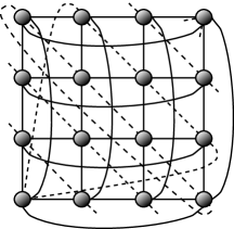
(a) Grids I and II

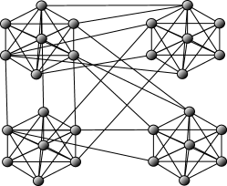
(b) Clustered graph

Figure 4: Examples of the test graph structures. The grid (a) was used with and without the dashed diagonal edges, and also with a variation of the connections in the first and last row. The clustered graphs were similar to the example shown in (b).

Cost functions.

The benchmark includes four families of functions. The first group (Matrix rank I,II, Labels I, II) consists of matroid rank functions or sums of three such functions. The functions used here are either based on matrix rank or ranks of partition matroids. We summarize those functions as rank-like costs.

The second group (Unstructured I, II) contains two variants of unstructured functions $g(w(C))$, where $g$ is either a logarithm or a square root. These functions are designed to favor a certain random optimal cut. The construction ensures that the minimum cut will not be one that separates out a single node, but one that cuts several edges.

The third family (Bestcut I, II) is constructed to make a cut optimal that has many edges and that is therefore different from the cut that uses fewest edges. For such a cut, we expect $\hat{f}_{add}$ to yield relatively poor solutions.

The fourth set of functions (Truncated rank) is inspired by the difficult truncated functions that can be used to establish lower bounds on approximation factors. These functions “hide” an optimal set, and interactions are only visible when guessing a large enough part of this hidden set. The following is a detailed description of all cost functions:

Matrix rank I.

Each element $e\in\mathcal{E}$ indexes a column in matrix $\mathbf{X}\in\mathbb{R}^{d\times m}$. The cost of $A\subseteq\mathcal{E}$ is the rank of the sub-matrix $\mathbf{X}_{A}$ of the columns indexed by the $e\in A$: $f_{\text{mrI}}(A)=\mathrm{rank}(\mathbf{X}_{A})$. The matrix $\mathbf{X}$ is of the form $[\;\mathbf{I^{\prime}}\;\;\mathbf{R}\;]$, where $\mathbf{R}\in\{0,1\}^{d\times(m-d)}$ is a random binary matrix with $d=0.9\sqrt{m}$, and $\mathbf{I}^{\prime}$ is a column-wise permutation of the identity matrix.

Matrix rank II.

The function $f_{\text{mrII}}(A)=0.33\sum_{i=1}^{3}f^{(i)}_{\text{mrI}}(A)$ sums up three functions $f^{(i)}_{\text{mrI}}$ of type matrix rank I with different random matrices $\mathbf{X}$.

Labels I.

This class consists of functions of the form $f_{\ell\text{I}}(A)=|\bigcup_{e\in A}\ell(e)|$. Each element $e$ is assigned a random label $\ell(e)$ from a set of $0.8\sqrt{m}$ possible labels. The cost counts the number of labels in $A$.

Labels II.

These functions $f_{\ell\text{II}}(A)=0.33\sum_{i=1}^{3}f^{(i)}_{\ell\text{I}}(A)$ are the sum of three functions of type labels I with different random labels.

Unstructured I.

These are functions $f_{\text{dpI}}(A)=\log{\sum_{e\in A}w(e)}$, where weights $w(e)$ are chosen randomly as follows. Sample a set $X\subset V$ with $|X|=0.4n$, and set $w(e)=1.001$ for all $e\in\delta X$. Then randomly assign some “heavy” weights in $[n/2,n^{2}/4]$ to some edges not in $\delta X$, so that each node is incident to one or two heavy edges. The remaining edges get random (mostly integer) weights between $1.001$ and $n^{2}/4-n+1$.

Unstructured II.

These are functions $f_{\text{dpII}}(A)=\sqrt{\sum_{e\in A}w(e)}$ with weights assigned as for unstructured function II.

Bestcut I.

We randomly pick a connected subset $X^{*}\subseteq\mathcal{V}$ of size $0.4n$ and define the cost $f_{\text{bcI}}(A)=\mathbf{1}[|A\cap\delta X^{*}|\geq 1]+\sum_{e\in A\setminus\delta X^{*}}w(e)$. The edges in $\mathcal{E}\setminus\delta X^{*}$ are assigned random weights $w(e)\in[1.5,2]$. If there is still a cut $C\neq\delta X^{*}$ with cost one or lower, we correct $w$ by increasing the weight of one $e\in C$ to $w(e)=2$. The optimal cut is then $\delta X^{*}$, but it is usually not the one with fewest edges.

Bestcut II.

Similar to bestcut I ($\delta X^{*}$ is again optimal), but with submodularity on all edges: $\mathcal{E}$ is partitioned into three sets, $E=(\delta X^{*})\cup B\cup C$. Then $f_{\text{bcII}}(A)=\mathbf{1}[|A\cap\delta X^{*}|\geq 1]+\sum_{e\in A\cap(B\cup C)}w(e)+\max_{e\in A\cap B}w(e)+\max_{e\in A\cap C}w(e)$. The weights of two edges in $B$ and two edges in $C$ are set to $w(e)\in(2.1,2.2)$.

Truncated rank.

This function is similar to the truncated rank in the proof of the lower bound (Theorem 1). Sample a connected $X\subseteq\mathcal{V}$ with $|X|=0.3|\mathcal{V}|$ and set $R=\delta X$. The cost is $f_{\text{tr}}(A)=\min\{|A\cap\overline{R}|+\min\{|A\cap R|,\lambda_{1}\},\;\lambda_{2}\}$ for $\lambda_{1}=\sqrt{|R|}$ and $\lambda_{2}=2|R|$. Here, $R$ is not necessarily the optimal cut.

To estimate the approximation factor on one problem instance (one graph and one cost function), we divide by the cost of the best solution found by any of the algorithms, unless the optimal solution is known (this is the case for Bestcut I and II).

7.1.1 Results

Figure 5 shows average empirical approximation factors and also the worst observed factors. The first observation is that all algorithms remain well below their theoretical approximation bounds. That means the theoretical bounds are really worst-case results. For several instances we obtain optimal solutions.

grid graphs	clustered graphs
rank-like cost functions (average over 61 (left), 80 (right) instances)
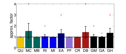
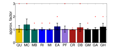
unstructured functions (average over 30 (left), 40 (right) instances)
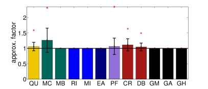
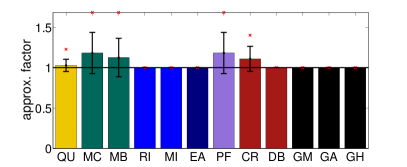
bestcut functions (average over 15 (left), 20 (right) instances)
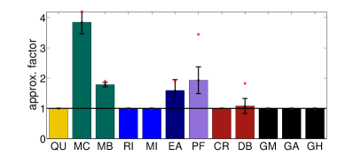
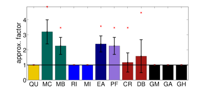
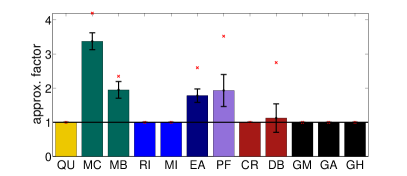
truncated rank (average over 15 (left), 20 (right) instances)

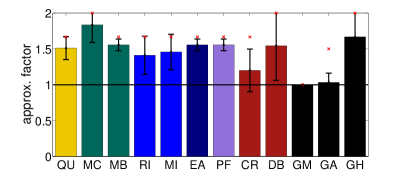
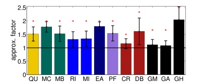
Figure 5: Results for average-case experiments. The bars show the mean empirical approximation factors, and red crosses mark the maximum observed empirical approximation factor. The left column refers to grid graphs, the right column to clustered graphs. The first three algorithms (bars) are baselines, the next four approximate $f$, the next four solve a relaxation, and the last is the deterministic greedy heuristic.

The general performance depends much on the actual problem instance; the truncated rank functions with hidden structure are, as may be expected, the most difficult. The simple benchmarks relying on $\hat{f}_{add}$ perform worse than the more sophisticated algorithms. Queyranne’s algorithm performs surprisingly well here.

7.2 Difficult instances

Lastly, we show two difficult instances. More examples may be found in (Jegelka, 2012, Ch. 4). The example demonstrates the drawbacks of using approximations like $\hat{f}_{add}$ and Queyranne’s algorithm.

Our instance is a graph with $n=10$ modes, shown in Figure 6. The graph edges are partitioned into $n/2$ sets, indicated by colors. The black set $\mathcal{E}_{k}$ makes up the cut with the maximum number of edges. The remaining edge sets are constructed as

$$\mathcal{E}_{i}=\big{\{}(v_{i},v_{j})\in\mathcal{E}\;|\;i<j\leq n/2\big{\}}\cup\big{\{}(v_{n/2+i},v_{j})\in\mathcal{E}\;|\;n/2+i<j\leq n\big{\}}$$ (42)

for each $1\leq i<n/2$. In Figure 6, set $\mathcal{E}_{1}$ is red, set $\mathcal{E}_{2}$ is blue, and so on. The cost function is

$$f_{a}(A)=\mathbf{1}\big{[}|A\cap\mathcal{E}_{k}|\geq 1\big{]}+\sum_{i=1}^{n/2-1}b\cdot\mathbf{1}\big{[}|A\cap\mathcal{E}_{i}|\geq 1\big{]}+\epsilon|A\cap\mathcal{E}_{k}|,$$ (43)

with $b=n/2$. The function $\mathbf{1}[\cdot]$ denotes the indicator function. The cost of the optimal solution is $f(C^{*})=f(\mathcal{E}_{k})=1+\frac{n^{2}}{4}\epsilon\approx 1$. The second-best solution is the cut $\delta(v_{1})$ with cost $f(\delta v_{1})=1+\frac{n^{2}}{4}\epsilon+b\approx 1+\frac{n}{2}=6$, i.e., it is by a factor of almost $b=n/2$ worse than the optimal solution. Finally, MC finds the solution $\delta(v_{n})$ with $f(\delta v_{n})=1+\frac{n^{2}}{4}\epsilon+b(\frac{n}{2}-1)\approx\frac{n^{2}}{4}=21$.

Variant (b) uses the cost function

$$f_{b}(A)=\mathbf{1}[|A\cap\mathcal{E}_{k}|\geq 1]+\sum_{i=1}^{n/2-1}b\cdot\mathbf{1}[|A\cap\mathcal{E}_{i}|\geq 1]$$ (44)

with a large constant $b=n^{2}=100$. For any $b>n/2$, any solution other than $C^{*}$ is more than $n^{2}/4=|C^{*}|>n$ times worse than the optimal solution. Hence, thanks to the upper bounds on their approximation factors, all algorithms except for QU find the optimal solution. The result of the latter depends on how it selects a minimizer of $f(B\cup e)-f(e)$ in the search for a pendent pair; this quantity often has several minimizers here. Variant (b) uses a specific adversarial permutation of node labels, for which QU always returns the same solution $\delta v_{1}$ with cost $b+1$, no matter how large $b$ is: its solution can become arbitrarily poor.

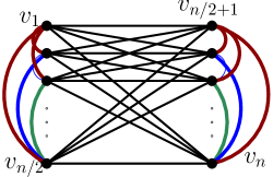
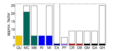
(a)		(b)

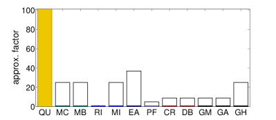
Figure 6: Difficult instance and empirical approximation factors with $n=10$ nodes. White bars illustrate theoretical approximation bounds where applicable. In (b), the second-best cut $\delta v_{1}$ has cost $f_{b}(\delta v_{1})=b+1=101\gg\max\{|C^{*}|,n,\sqrt{m}\log m\}$.

8 Discussion

In this work, we have defined and analyzed the MinCoopCut problem, that is, a minimum $(s,t)$-cut problem with a submodular cost function on graph edges. This problem unifies a number of non-additive graph cut problems in the literature that have arisen in different application areas.

We showed an information-theoretic lower bound of $\Omega(\sqrt{n})$ for the general MinCoopCut problem if the function is given as an oracle, and NP-hardness even if the cost function is fully known and polynomially representable. We propose and compare complementary approximation algorithms that either rely on representing the cost function by a simpler function, or on solving a relaxation of the mathematical program. The latter are closely tied to the longest path of cooperating edges in the graph, as is the flow-cut gap. We also show that the flow-cut gap may be as large as $n-1$, and therefore larger than the best approximation factor possible.

The lower bound and analysis of the integrality gap use a particular graph structure, a graph with parallel disjoint paths of equal length. Taken all proposed algorithms together, all instances of MinCoopCut on graphs with parallel paths of the same length can be solved within an approximation bound at most $\sqrt{n}$. This leaves the question whether there is an instance that makes all approximations worse than $\sqrt{n}$.

Section 6 outlined properties of submodular functions that facilitate submodular minimization under combinatorial constraints, and also submodular minimization in general. Apart from separability, we defined the hierarchy of function classes $\mathcal{F}(k)$. The $\mathcal{F}(k)$ are related to graph-representability and might therefore build a bridge between recent results about limitations of representing submodular functions as graph cuts (Z̆ivný et al., 2009) (and, even stricter, the limitations of polynomial representability) and the results discussed in Section 6.2 that provide improved algorithms whose complexity depends on $k$.

8.1 Open problems

This paper is part of a growing collection of work that studies submodular cost functions in combinatorial optimization problems over cuts, trees, matchings, and so on. Such problems are not only of theoretical interest: they occur in a spectrum of problems in computer vision (Jegelka and Bilmes, 2011a; Shelhamer et al., 2014; Heng et al., 2015; Taniai et al., 2015) and machine learning (Iyer et al., 2013a; Iyer and Bilmes, 2013; Khalil et al., 2014). In several cases, the functions used do not directly fall into any of the “easier” sub-classes (e.g., the entropy cuts outlined in Section 2, and also see the discussion in Section 2.3). At the same time, the empirical results in this paper and others (Iyer et al., 2013a) suggest that in many cases, the results of approximate algorithms can still be good, even though in the worst case they are not. Section 6 outlines beneficial properties. Is there a more precise quantification of the complexity of these problems? Do there exist other properties that lead to better algorithms? One direction that is less explored is the interaction of the graph structure with the cost function.

Specific to this work, cut functions induce a function on nodes. Propositions 2 and 3 imply that the node function can be submodular, but in very many cases it is not. Yet, the results for Queyranne’s algorithm in Section 7 suggest that often the function $h$ may remain close to submodular. This could be the case, for example, if the graph is almost complete and $f$ symmetric, or if the symmetry of $f$ is more restricted. A deeper study of the functions $h$ induced by cooperative cuts could reveal insights about a refined complexity of the problem, and explain the good empirical results. One particular interesting example was the polymatroidal flow case where the function $f$ defined in Eqn. (28) was not necessarily submodular (see Proposition 5), but where the resulting $h$ (also not necessarily submodular) could be optimized exactly in polynomial time. This suggests an interesting future direction, namely to fully characterize a class of functions $f$ for which polytime algorithms can be obtained to solve minimum “interacting cut” problems (i.e., cut problems where the edges may interact but not necessarily in a purely submodular or supermodular fashion). The dual polymatroidal flow case shows one instance of interacting cut that can be solved exactly.

Finally, finding optimal bounds and algorithms for related cut problems with submodular edge weights is an open problem. Appendix A outlines some initial results for cooperative multi-way and sparsest cut.

Appendix A Cooperative multi-cut and sparsest cut

An extension of MinCoopCut is the problem of cooperative multi-way cut and sparsest cut. Using the approximation $\hat{f}_{ea}$ from Section 5.1.3, we can transform any multi-way or sparsest cut problem with a submodular cost function on edges (instead of a sum of edge weights) into a cut problem whose cut cost is a convolution of local submodular functions. The relaxation of this cut problem is dual to the polymatroidal flow problems considered by Chekuri et al. [2012]. Combining their results with ours, we get the following Lemma.

Lemma 11.

Let $\alpha$ be the approximation factor for solving a sparsest cut / multi-way cut in a polymatroidal network. If we solve a cooperative sparsest cut / multi-way cut by first approximating the cut cost $f$ by a function $\hat{f}_{ea}$ and, on this instance, using the method with factor $\alpha$, we get an $O(\alpha n)$-approximation for cooperative sparsest cut / multi-way cut.

Using Theorems 6 and 8 in [Chekuri et al., 2012], we obtain the following bounds:

Corollary 2.

There is an $O(n\log k)$ approximation for cooperative sparsest cut in undirected graphs that is dual to a maximum multicommodity flow problem with $k$ pairs, and an $O(n\log k)$ approximation for cooperative multi-way cut.

We leave it as an open problem whether these bounds are optimal.

Appendix B Proof of Proposition 2

The first part of Proposition 2 is proven by Figure 1. Here, we show the second part that the function $h(X)=f(\delta^{+}(X))$ is subadditive if $f$ is nondecreasing and submodular. Let $X,Y\subseteq\mathcal{V}$. Then it holds that

$$h(X)+h(Y) =f(\delta^{+}(X))+f(\delta^{+}(Y))$$ (45)

$$\geq f(\delta^{+}(X)\cup\delta^{+}(Y))+f(\delta^{+}(X)\cap\delta^{+}(Y))$$ (46)

$$\geq f(\delta^{+}(X)\cup\delta^{+}(Y))$$ (47)

$$\geq f(\delta^{+}(X\cup Y))$$ (48)

$$=h(X\cup Y).$$ (49)

In Inequality (46), we used that $f$ is submodular, and in Inequality (47), we used that $f$ is nonnegative.

Appendix C Reduction from Graph Bisection to MinCoopCut

In this section, we prove Theorem 2 via a reduction from Graph Bisection, which is known to be NP-hard [Garey et al., 1976].

Definition 2 (Graph Bisection).

Given a graph $\mathcal{G}_{B}=(\mathcal{V}_{B},\mathcal{E}_{B})$ with edge weights $w_{B}:\mathcal{E}_{B}\to\mathbb{R}_{+}$, find a partition $V_{1}\dot{\cup}V_{2}=\mathcal{V}_{B}$ with $|V_{1}|=|V_{2}|=|\mathcal{V}_{B}|/2$ with minimum cut weight $w(\delta(V_{1}))$.

Proof.

To reduce Graph Bisection to MinCoopCut, we construct an auxiliary graph $\mathcal{G}=(\mathcal{V}_{B}\cup\{s,t\},\mathcal{E}_{B}\cup\mathcal{E}_{s}\cup\mathcal{E}_{t})$ that contains an unchanged copy of $\mathcal{G}_{B}$ and two additional terminal nodes $s,t$. The submodular weights on the edges adjacent to the terminal nodes will express the balance constraint $|V_{1}|=|V_{2}|=|\mathcal{V}_{B}|/2$.

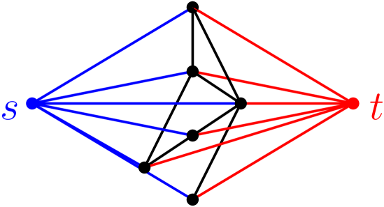
(a) graph $\mathcal{G}$ with $\mathcal{E}_{s}$ (blue), $\mathcal{E}_{t}$ (red) and $\mathcal{G}_{B}$ (black)

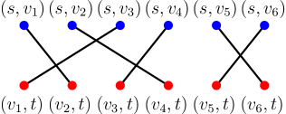
(b) graph $\mathcal{H}_{\sigma}$

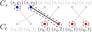
(c) $h_{\sigma}(\phi(C))=5$ connected components

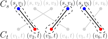
(d) balanced cut $C$: $h_{\sigma}(\phi(C))=3$ connected components

Figure 7: Graph for the reduction and examples for the definition of $f_{bal}$ via ranks $h_{\sigma}$, with $n_{B}=6$. In (c), $C_{s}=\{(s,v_{1}),(s,v_{2})\}$ and $C_{t}=\{(v_{3},t),(v_{4},t),(v_{5},t),(v_{6},t)\}$; in (d), $C_{s}=\{(s,v_{1}),(s,v_{4}),(s,v_{5})\}$ and $C_{t}=\{(v_{2},t),(v_{3},t),(v_{6},t)\}$. Connected components are indicated by dashed lines.

In $\mathcal{G}$, we retain the modular costs $w$ on $\mathcal{E}_{B}$ and connect $s,t$ to every vertex in $\mathcal{G}_{B}$ with corresponding new edge sets $\mathcal{E}_{s}$ and $\mathcal{E}_{t}$, as illustrated in Figure 7(a). The cost of a cut in $\mathcal{G}$ is measured by the submodular function

$$f(C)=\sum_{e\in C\cap\mathcal{E}_{B}}w(e)+\beta f_{bal}(C\cap(\mathcal{E}_{s}\cup\mathcal{E}_{t})),$$ (50)

where $\beta$ is an appropriately large constant, and $f_{bal}$ will be defined later. Obviously, any minimal $(s,t)$-cut $C$ must include $n_{B}=|\mathcal{V}_{B}|$ edges from $\mathcal{E}_{s}\cup\mathcal{E}_{t}$, and partitions $\mathcal{V}_{B}$. Moreover, the cardinality of $C_{s}=C\cap\mathcal{E}_{s}$ is the number of nodes in $\mathcal{V}_{B}$ assigned to $t$. Hence, in an equipartition, $|C_{s}|=|C_{t}|=n_{B}/2$, where $C_{t}=C\cap\mathcal{E}_{t}$.

It remains to define $f_{bal}$ as a nondecreasing submodular function that implements the equipartition constraint. The function will be an expectation over matroid rank functions $h_{\sigma}$. Let $\mathcal{H}_{\sigma}=(\mathcal{E}_{s},\mathcal{E}_{t},\mathcal{F}_{\sigma})$ be a bipartite graph with nodes $\mathcal{E}_{s}\cup\mathcal{E}_{t}$ whose edges $\mathcal{F}_{\sigma}$ form a derangement between $\mathcal{E}_{s}$ and $\mathcal{E}_{t}$, as illustrated in Fig. 7(b).

Let $\phi(C_{s}\cup C_{t})$ be the image of $C_{s}\cup C_{t}$ in the set of nodes of $\mathcal{H}_{\sigma}$. The function $h_{\sigma}:2^{\phi(\mathcal{E}_{s}\cup\mathcal{E}_{t})}\to\mathbb{N}_{0}$ counts the number of connected components in the subgraph induced by the nodes $\phi(C_{s}\cup C_{t})$, and is the rank of a partition matroid. Figure 7 shows some examples.

Let $\mathfrak{S}$ be the set of all derangements $\sigma$ of $n_{B}$ elements, i.e., all possible edge configurations in $\mathcal{H}_{\sigma}$. We define $f_{bal}$ to be the expectation (under uniform draws of $\sigma$)

$$f_{bal}(C)=\mathbb{E}_{\sigma}[h_{\sigma}(\phi(C))]=|\mathfrak{S}|^{-1}\sum\nolimits_{\sigma\in\mathfrak{S}}h_{\sigma}(\phi(C)).$$ (51)

For a fixed derangement $\sigma^{\prime}$ and a fixed size $|C_{s}\cup C_{t}|=n_{B}$, the value $h_{\sigma^{\prime}}(C_{s}\cup C_{t})$ is minimal if $\sigma^{\prime}(C_{s})=C_{t}$ and $|C_{s}|=|C_{t}|$. For a fixed $\sigma$, the rank $h_{\sigma}(C)$ is $|\phi(C_{s}\cup C_{t})|=|C_{s}|+|C_{t}|$ minus the matching nodes. Denoting $(s,v_{i})$ in $\mathcal{H}_{\sigma}$ by $x_{i}$ and $(v_{i},t)$ by $y_{i}$, the rank is

$$h_{\sigma}(\phi(C_{s})\cup\phi(C_{t})) =|C_{s}|+|C_{t}|-{\Big{|}\big{\{}(x_{i},y_{\sigma(i)})\big{\}}_{i=1}^{n}\;\cap\;(\phi(C_{s})\times\phi(C_{t}))\Big{|}}.$$ (52)

Hence, the sum in (51) becomes

$$\sum_{\sigma\in\mathfrak{S}}h_{\sigma}(C) =|\mathfrak{S}|\big{(}|C_{s}|+|C_{t}|\big{)}-\sum_{\sigma\in\mathfrak{S}}\big{|}\big{\{}(x_{i},y_{\sigma(i)})\big{\}}_{i=1}^{n}\,\cap\,(\phi(C_{s})\times\phi(C_{t}))\big{|}$$ (53)

$$=|\mathfrak{S}|\big{(}|C_{s}|+|C_{t}|\big{)}-\sum_{x_{i}\in\phi(C_{s})}\sum_{\sigma\in\mathfrak{S}}\big{|}(x_{i},y_{\sigma(i)})\cap(\{x_{i}\}\times\phi(C_{t}))\big{|}$$ (54)

To compute the sum over $\sigma$ in the second term, let $C_{s\cap t}\triangleq\{(s,v)\,|\,\{(s,v),(v,t)\}\subseteq C\}$ be the set of $s$-edges whose counterpart on the $t$ side is also contained in $C$. Let further $D^{\prime}(n_{B}-1)$ denote the number of permutations of $n_{B}-1$ elements (pair $(x_{i},y_{k})$, i.e., $\sigma(i)=k$, is fixed), where one specific element $x_{k}$ can be mapped to any other of the $n_{B}-1$ elements, and the remaining elements must not be mapped to their counterparts ($\sigma(j)\neq j$). Then there are $D^{\prime}(n_{B}-1)$ derangements $\sigma$ realizing a specific mapping $\sigma(i)=k$. Denoting the number of derangements of $n$ elements by $D(n)$, the sum above becomes

$$D(n_{B})f_{bal}(C) =(|C_{s}|+|C_{t}|)D(n_{B})$$ (55)

$$\quad\quad-\sum_{x_{i}\in C_{s}\setminus C_{s\cap t}}\sum_{y_{k}\in C_{t}}D^{\prime}(n_{B}-1)-\sum_{x_{i}\in C_{s\cap t}}\sum_{y_{k}\in C_{t},k\neq i}D^{\prime}(n_{B}-1)$$

$$=(|C_{s}|+|C_{t}|)D(n_{B})$$ (56)

$$\quad\quad-\big{(}|C_{s}|-|C_{s\cap t}|\big{)}|C_{t}|D^{\prime}(n_{B}-1)-|C_{s\cap t}|(|C_{t}|-1)D^{\prime}(n_{B}-1)$$

$$=(|C_{s}|+|C_{t}|)D(n_{B})-(|C_{s}||C_{t}|-|C_{s\cap t}|)D^{\prime}(n_{B}-1),$$ (57)

with $D(n)=|\mathfrak{S}|=n!\sum_{k=0}^{n}(-1)^{k}/k!$ [Stanley, 1997], and $D^{\prime}(n-1)=\sum_{k=0}^{n-1}(n-2)!(n-1-k)!(-1)^{k}$ by Proposition 4 below.

Given that $|C_{s}|+|C_{t}|$ must cut at least $n_{B}$ edges and that $f_{bal}$ is increasing, $f_{bal}$ is minimized if $|C_{s}|=|C_{t}|=n_{B}/2$. As a result, if $\beta$ is large enough such that $f_{bal}$ dominates the cost, then a minimum cooperative cut in $\mathcal{G}$ bisects the $\mathcal{G}_{B}$ subgraph of $\mathcal{G}$ optimally. ∎∎

Proposition 4.

Let $D^{\prime}(n)$ be the number of permutations of $n$ elements where for one fixed element $i^{\prime}$ we allow $\sigma(i^{\prime})\in\{1,\ldots,n\}$, but $\sigma(i)\neq i$ for all $i\neq i^{\prime}$. Then $D^{\prime}(n)=\sum_{k=0}^{n}\frac{(n-1)!}{k!}(n-k)!(-1)^{k}$.

Proof.

$D^{\prime}(n)$ can be derived by the method of the forbidden board [Stanley, 1997, pp. 71-73]. Let, without loss of generality, $i^{\prime}=n$, so the forbidden board is $B=\{(1,1),(2,2),\ldots,(n-1,n-1)\}$. Let $N_{j}$ be the number of permutations $\sigma$ for which $\big{|}\{(i,\sigma(i)\}_{i=1}^{n}\cap B\big{|}=j$, and let $r_{k}$ be the number of $k$-subsets of $B$ such that no two elements have a coordinate in common. Here, $r_{k}~{}=~{}{n-1\choose k}$. Then $D^{\prime}(n)=N_{0}=N_{n}(0)$ for

$$N_{n}(x) =\sum_{j}N_{j}x^{j}=\sum_{k=0}^{n}r_{k}(n-k)!(x-1)^{k}=\sum_{k=0}^{n}\frac{(n-1)!}{k!}(n-k)(x-1)^{k},$$ (58)

and hence $D^{\prime}(n)=\sum_{k=0}^{n}\frac{(n-1)!}{k!}(n-k)!(-1)^{k}$. ∎

Appendix D Convolutions of submodular functions are not always submodular

The non-submodularity of convolutions was mentioned already in [Lovász, 1983]. For completeness, we show an explicit example that illustrates that non-submodularity also holds for the special case of polymatroidal flows.

Proposition 5.

The convolution of two submodular functions $(f\ast g)(A)=\min_{B\subseteq A}f(B)+g(A\setminus B)$ is not in general submodular. In particular, this also holds for the cut cost functions occurring in the dual problems of polymatroidal maximum flows.

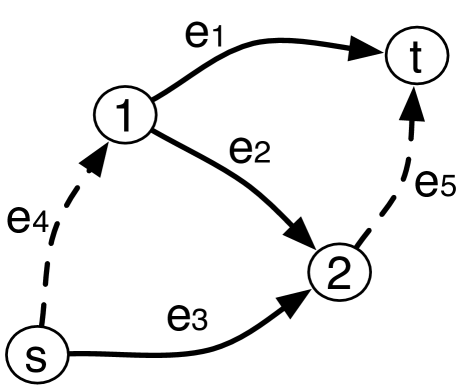
Let $f(A)=\max_{e\in A}w(e)$ and

$w(e_{1})=w(e_{2})=a$,

$w(e_{3})=b$,

$w(e_{4})=w(e_{5})=\epsilon$.

Figure 8: Example showing that the convolution of submodular functions is not always submodular, e.g., for $a=1.5$, $b=2$ and $\epsilon=0.001$.

To show Proposition 5, consider the graph in Figure 5 with a submodular edge cost function $f(A)=\max_{e\in A}w(e)$. The two submodular functions that are convolved in the corresponding polymatroidal flow are the decompositions

$$\mathrm{cap}^{\text{out}}(A) =\sum_{v\in\mathcal{V}}f(A\cap\delta^{+}(v))$$ (59)

$$\mathrm{cap}^{\text{in}}(A) =\sum_{v\in\mathcal{V}}f(A\cap\delta^{-}(v)).$$ (60)

Both $\mathrm{cap}^{\text{out}}$ and $\mathrm{cap}^{\text{in}}$ are submodular functions from $2^{\mathcal{E}}$ to $\mathbb{R}_{+}$. Their convolution $h$ is

$$h(A)=(\mathrm{cap}^{\text{out}}\ast\mathrm{cap}^{\text{in}})(A)=\min_{B\subseteq A}\mathrm{cap}^{\text{out}}(B)+\mathrm{cap}^{\text{in}}(A\setminus B)=\hat{f}_{pf}(A).$$ (61)

For $h$ to be submodular, it must satisfy the condition of diminishing marginal costs, i.e., for any $e$ and $A\subseteq B\subseteq\mathcal{E}\setminus e$, it must hold that $h(e\mid A)\geq h(e\mid B)$. Now, let $A=\{e_{2}\}$ and $B=\{e_{1},e_{2}\}$. The convolution here means to pair $e_{3}$ either with $e_{1}$ or $e_{2}$. Then, if $a<b$,

$$h(e_{3}\mid A) =\min\{a+b,b\}-a=b-a$$ (62)

$$h(e_{3}\mid B) =a+b-\min\{a+a,a\}=b.$$ (63)

Hence, $h(e_{3}\mid A)<h(e_{3}\mid B)$, disproving submodularity of $h$.

Appendix E Cooperative Cuts and Polymatroidal Networks

We next prove Lemma 6 that relates the approximation $\hat{f}_{pf}$ to maxflow problems in polymatroidal networks.

Proof.

(Lemma 6) The first step is the dual of the polymatroidal flow. Let $\mathrm{cap}^{\text{in}}:2^{\mathcal{E}}\to\mathbb{R}_{+}$ be the joint incoming capacity, $\mathrm{cap}^{\text{in}}(C)=\sum_{v\in V}\mathrm{cap}_{v}^{\text{in}}(C\cap\delta^{-}v)$, and let equivalently $\mathrm{cap}^{\text{out}}$ be the joint outgoing capacity. The dual of the polymatroidal maximum flow is a minimum cut problem whose cost is a convolution of edge capacities [Lovász, 1983]:

$$\mathrm{cap}(C)=(\mathrm{cap}^{\text{in}}\ast\mathrm{cap}^{\text{out}})(C)\;\triangleq\;\min_{A\subseteq C}\bigl{[}\mathrm{cap}^{\text{in}}(A)+\mathrm{cap}^{\text{out}}(C\setminus A)\bigr{]}.$$ (64)

We will relate this dual to the approximation $\hat{f}_{pf}$. Given a minimal $(s,t)$-cut $C$, let $\Pi(C)$ be a partition of $C$, and $C_{v}^{\text{in}}=C^{\Pi}_{v}\cap\delta^{-}_{v}$ and $C_{v}^{\text{out}}=C^{\Pi}_{v}\cap\delta^{+}_{v}$. The cut $C$ partitions the nodes into two sets $\mathcal{V}_{s}$ containing $s$ and $\mathcal{V}_{t}$ containing $t$. Since $C$ is a minimal directed cut, it contains only edges from the $s$ side $\mathcal{V}_{s}$ to the $t$ side $\mathcal{V}_{t}$ of the graph. In consequence, $C_{v}^{\text{in}}=\emptyset$ if $v$ is on the $s$ side, and $C_{v}^{\text{out}}=\emptyset$ otherwise. Hence, $C^{\text{in}}_{v}\cup C^{\text{out}}_{v}$ is equal to either $C^{\text{in}}_{v}$ or $C^{\text{out}}_{v}$, and since $f(\emptyset)=0$, it holds that $f(C^{\text{in}}_{v}\cup C^{\text{out}}_{v})=f(C^{\text{in}}_{v})+f(C^{\text{out}}_{v})$. Then, starting with the definition of $\hat{f}_{pf}$,

$$\hat{f}_{pf}(C) =\min_{\Pi(C)\in\mathcal{P}_{C}}\sum\nolimits_{v\in\mathcal{V}}f(C^{\Pi}_{v})$$ (65)

$$=\min_{\Pi(C)\in\mathcal{P}_{C}}\sum\nolimits_{v\in\mathcal{V}}f(C^{\text{in}}_{v}\cup C^{\text{out}}_{v})$$ (66)

$$=\min_{\Pi(C)\in\mathcal{P}_{C}}\sum\nolimits_{v\in\mathcal{V}}\bigl{[}f(C^{\text{in}}_{v})+f(C^{\text{out}}_{v})\bigr{]}$$ (67)

$$=\min_{\Pi(C)\in\mathcal{P}_{C}}\sum\nolimits_{v\in\mathcal{V}}\bigl{[}\mathrm{cap}_{v}^{\text{in}}(C^{\text{in}}_{v})+\mathrm{cap}_{v}^{\text{out}}(C^{\text{out}}_{v})\bigr{]}$$ (68)

$$=\min_{C^{\text{in}},C^{\text{out}}}\bigl{[}\mathrm{cap}^{\text{in}}(C^{\text{in}})+\mathrm{cap}^{\text{out}}(C^{\text{out}})\bigr{]}$$ (69)

$$=\min_{C^{\text{in}}\subseteq C}\bigl{[}\mathrm{cap}^{\text{in}}(C^{\text{in}})+\mathrm{cap}^{\text{out}}(C\setminus C^{\text{in}})\bigr{]}$$ (70)

$$=(\mathrm{cap}^{\text{in}}\ast\mathrm{cap}^{\text{out}})(C).$$ (71)

The minimum in Equation (67) is taken over all feasible partitions $\Pi(C)$ and their resulting intersections with the sets $\delta^{+}v,\delta^{-}v$. Then we use the notation $C^{\text{in}}=\bigcup_{v\in\mathcal{V}}C_{v}^{\text{in}}$ for all edges assigned to their head nodes, and $C^{\text{out}}=\bigcup_{v\in\mathcal{V}}C_{v}^{\text{out}}$. The minima in Equations (69) and (70) are again taken over all partitions in $\mathcal{P}_{C}$. The final equality follows from the above definition of a convolution of submodular functions. ∎∎

References

- Ahuja et al. [1993] R. K. Ahuja, T. L. Magnanti, and J. B. Orlin. Network Flows. Prentice Hall, 1993.
- Allène et al. [2009] C. Allène, J.-Y. Audibert, M. Couprie, and R. Keriven. Some links between extremum spanning forests, watersheds, and min-cuts. Image and Vision Computing, 2009.
- Bagon [2006] S. Bagon. Matlab wrapper for graph cut, December 2006. http://www.wisdom.weizmann.ac.il/ bagon.
- Balcan and Harvey [2012] N. Balcan and N. Harvey. Submodular functions: Learnability, structure, and optimization. arXiv:0486478, 2012.
- Baumann et al. [2013] F. Baumann, S. Berckey, and C. Buchheim. Facets of Combinatorial Optimization — Festschrift for Martin Grötschel, chapter Exact Algorithms for Combinatorial Optimization Problems with Submodular Objective Functions, pages 271–294. Springer, 2013.
- Bilmes [2010] J. Bilmes. Dynamic graphical models – an overview. IEEE Signal Processing Magazine, 27(6):29–42, 2010.
- Bilmes and Bartels [2003] J. Bilmes and C. Bartels. On triangulating dynamic graphical models. In Uncertainty in Artificial Intelligence, pages 47–56, Acapulco, Mexico, 2003. Morgan Kaufmann Publishers.
- Boykov and Jolly [2001] Y. Boykov and M.-P. Jolly. Interactive graph cuts for optimal boundary and region segmentation of objects in n-d images. In Int. Conf. on Computer Vision (ICCV), 2001.
- Boykov and Kolmogorov [2004] Y. Boykov and V. Kolmogorov. An experimental comparison of min-cut/max-flow algorithms for energy minimization in vision. IEEE Trans. on Pattern Analysis and Machine Intelligence, 26(9):1124–1137, 2004.
- Boykov and Veksler [2006] Y. Boykov and O. Veksler. Handbook of Mathematical Models in Computer Vision, chapter Graph Cuts in Vision and Graphics: Theories and Applications. Springer, 2006.
- Bunke et al. [2007] F. Bunke, H. W. Hamacher, F. Maffioli, and A. Schwahn. Minimum cut bases in undirected networks. Report in Wirtschaftsmathematik (WIMA Report) 108, Universität Kaiserslautern, 2007.
- Chambolle and Darbon [2009] A. Chambolle and J. Darbon. On total variation minimization and surface evolution using parametric maximum flows. Int. Journal of Computer Vision, 84(3), 2009.
- Chekuri et al. [2012] C. Chekuri, S. Kannan, A. Raja, and P. Viswanath. Multicommodity flows and cuts in polymatroidal networks. In Innovations in Theoretical Computer Science (ITCS), 2012.
- Conforti and Cornuéjols [1984] M. Conforti and G. Cornuéjols. Submodular set functions, matroids and the greedy algorithm: tight worst-case bounds and some generalizations of the Rado-Edmonds theorem. Discrete Applied Mathematics, 7(3):251–274, 1984.
- Couprie et al. [2011] C. Couprie, L. Grady, H. Talbot, and L. Najman. Combinatorial continuous maximum flow. SIAM Journal on Imaging, pages 905–930, 2011.
- Cunningham [1983] W. H. Cunningham. Decomposition of submodular functions. Combinatorica, 3(1):53–68, 1983.
- Dantzig and Fulkerson [1955] G. Dantzig and D. Fulkerson. On the max flow min cut theorem of networks. Technical Report P-826, The RAND Corporation, 1955.
- Ene et al. [2013] A. Ene, J. Vondrák, and Y. Wu. Local distribution and the symmetry gap: Approximability of multiway partitioning problems. In Proc. SIAM-ACM Symp. on Discrete Algorithms (SODA), 2013.
- Fix et al. [2013] A. Fix, T. Joachims, S. M. Park, and R. Zabih. Structured learning of sum-of-submodular higher order energy functions. In Int. Conf. on Computer Vision (ICCV), 2013.
- Ford and Fulkerson [1956] L. Ford and D. Fulkerson. Maximal flow through a network. Canadian Journal of Mathematics, 8:399–404, 1956.
- Garey et al. [1976] M. R. Garey, D. S. Johnson, and L. Stockmeyer. Some simplified NP-complete graph problems. Theoretical Computer Science, 1(3):237–267, 1976.
- Goel et al. [2009] G. Goel, C. Karande, P. Tripati, and L. Wang. Approximability of combinatorial problems with multi-agent submodular cost functions. In Proc. IEEE Symp. on Foundations of Computer Science (FOCS), 2009.
- Goel et al. [2010] G. Goel, P. Tripathi, and L. Wang. Combinatorial problems with discounted price functions in multi-agent systems. In Foundations of Software Technology and Theoretical Computer Science (FSTTCS), 2010.
- Goemans et al. [2009] M. Goemans, N. J. A. Harvey, S. Iwata, and V. S. Mirrokni. Approximating submodular functions everywhere. In Proc. SIAM-ACM Symp. on Discrete Algorithms (SODA), 2009.
- [25] M. X. Goemans, N. J. A. Harvey, R. Kleinberg, and V. S. Mirrokni. On learning submodular functions – a preliminary draft. Unpublished Manuscript.
- Goyal and Ravi [2008] V. Goyal and R. Ravi. An FPTAS for minimizing a class of low-rank quasi-concave functions over a convex domain. Technical Report 366, Tepper School of Business, Carnegie Mellon University, 2008.
- Greig et al. [1989] D. M. Greig, B. T. Porteous, and A. H. Seheult. Exact maximum a posteriori estimation for binary images. Journal of the Royal Statistical Society, 51(2), 1989.
- Hassin [1982] R. Hassin. Minimum cost flow with set constraints. Networks, 12:1–21, 1982.
- Hassin et al. [2007] R. Hassin, J. Monnot, and D. Segev. Approximation algorithms and hardness results for labeled connectivity problems. J. Comb. Optim., 14(4):437–453, 2007.
- Heng et al. [2015] L. Heng, A. Gotovos, A. Krause, and M. Pollefeys. Efficient visual exploration and coverage with a micro aerial vehicle in unknown environments. In IEEE Int. Conf. on Robotics and Automation (ICRA), 2015.
- Iwata and Nagano [2009] S. Iwata and K. Nagano. Submodular function minimization under covering constraints. In Proc. IEEE Symp. on Foundations of Computer Science (FOCS), 2009.
- Iyer and Bilmes [2013] R. Iyer and J. Bilmes. Submodular optimization with submodular cover and submodular knapsack constraints. In Neural Information Processing Society (NIPS), 2013.
- Iyer et al. [2013a] R. Iyer, S. Jegelka, and J. Bilmes. Fast semidifferential-based submodular function optimization. In Proc. Int. Conf. on Machine Learning (ICML), 2013a.
- Iyer et al. [2013b] R. Iyer, S. Jegelka, and J. Bilmes. Curvature and optimal algorithms for learning and minimizing submodular functions. In Neural Information Processing Society (NIPS), 2013b.
- Jegelka [2012] S. Jegelka. Combinatorial Problems with submodular coupling in machine learning and computer vision. PhD thesis, ETH Zurich, 2012.
- Jegelka and Bilmes [2011a] S. Jegelka and J. Bilmes. Submodularity beyond submodular energies: coupling edges in graph cuts. In IEEE Conf. on Computer Vision and Pattern Recognition (CVPR), 2011a.
- Jegelka and Bilmes [2011b] S. Jegelka and J. Bilmes. Approximation bounds for inference using cooperative cuts. In Proc. Int. Conf. on Machine Learning (ICML), 2011b.
- Jegelka et al. [2011] S. Jegelka, H. Lin, and J. Bilmes. On fast approximate submodular minimization. In Neural Information Processing Society (NIPS), 2011.
- Jegelka et al. [2013] S. Jegelka, F. Bach, and S. Sra. Reflection methods for user-friendly submodular optimization. In Neural Information Processing Society (NIPS), 2013.
- Jha et al. [2002] S. Jha, O. Sheyner, and J. Wing. Two formal analyses of attack graphs. In Proc. of the 15th Computer Security Foundations Workshop, pages 49–63, 2002.
- Kannan and Viswanath [2011] S. Kannan and P. Viswanath. Multiple-unicast in fading wireless networks: A separation scheme is approximately optimal. In IEEE Int. Symposium on Information Theory (ISIT), 2011.
- Kannan et al. [2011] S. Kannan, A. Raja, and P. Viswanath. Local phy + global flow: A layering principle for wireless networks. In IEEE Int. Symposium on Information Theory (ISIT), 2011.
- Khalil et al. [2014] E. B. Khalil, B. Dilkina, and L. Song. Scalable diffusion-aware optimization of network topology. In Proceedings of the 20th ACM SIGKDD international conference on Knowledge discovery and data mining, pages 1226–1235. ACM, 2014.
- Kohli et al. [2009a] P. Kohli, M. Kumar, and P. Torr. P3 & beyond: Move making algorithms for solving higher order functions. IEEE Trans. on Pattern Analysis and Machine Intelligence, pages 1645–1656, 2009a.
- Kohli et al. [2009b] P. Kohli, L. Ladický, and P. Torr. Robust higher order potentials for enforcing label consistency. International Journal of Computer Vision, 82(3):302–324, 2009b.
- Kohli et al. [2013] P. Kohli, A. Osokin, and S. Jegelka. A principled deep random field for image segmentation. In IEEE Conf. on Computer Vision and Pattern Recognition (CVPR), 2013.
- Kolmogorov [2012] V. Kolmogorov. Minimizing a sum of submodular functions. Discrete Applied Mathematics, 160(15), 2012.
- Kolmogorov and Boykov [2005] V. Kolmogorov and Y. Boykov. What metrics can be approximated by geo-cuts, or global optimization of length/area and flux. In Int. Conf. on Computer Vision (ICCV), 2005.
- Kolmogorov and Zabih [2004] V. Kolmogorov and R. Zabih. What energy functions can be minimized via graph cuts? IEEE Trans. on Pattern Analysis and Machine Intelligence, 26(2):147–159, 2004.
- Koufogiannakis and Young [2009] C. Koufogiannakis and N. E. Young. Greedy -approximation algorithm for covering with arbitrary constraints and submodular costs. In Int. Colloquium on Automata, Languages and Programming (ICALP), 2009.
- Krause [2010] A. Krause. SFO: A toolbox for submodular function optimization. Journal of Machine Learning Research, 11:1141–1144, 2010.
- Lawler and Martel [1982] E. L. Lawler and C. U. Martel. Computing maximal “Polymatroidal” network flows. Mathematics of Operations Research, 7(3):334–347, 1982.
- Lin and Bilmes [2012] H. Lin and J. Bilmes. Learning mixtures of submodular shells with application to document summarization. In Uncertainty in Artificial Intelligence (UAI), 2012.
- Lovász [1983] L. Lovász. Mathematical programming – The State of the Art, chapter Submodular Functions and Convexity, pages 235–257. Springer, 1983.
- Mittal and Schulz [2012] S. Mittal and A. Schulz. An FPTAS for optimizing a class of low-rank functions over a polytope. Mathematical Programming, 2012.
- Mitzenmacher and Upfal [2005] M. Mitzenmacher and E. Upfal. Probability and Computing: Randomized Algorithms and Probabilistic Analysis. Cambridge University Press, 2005.
- Narayanan [1997] H. Narayanan. Submodular Functions and Electrical Networks. Elsevier Science, 1997.
- Nikolova [2010] E. Nikolova. Approximation algorithms for reliable stochastic combinatorial optimization. In APPROX, 2010.
- Queyranne [1998] M. Queyranne. Minimizing symmetric submodular functions. Mathematical Programming, 82:3–12, 1998.
- Ramalingam et al. [2008] S. Ramalingam, P. Kohli, K. Alahari, and P. Torr. Exact inference in multi-label CRFs with higher order cliques. In IEEE Conf. on Computer Vision and Pattern Recognition (CVPR), 2008.
- Ramalingam et al. [2011] S. Ramalingam, C. Russell, L. Ladicky, and P. H. S. Torr. Efficient minimization of higher order submodular functions using monotonic boolean functions. ArXiv 1109.2304, 2011.
- Rudin et al. [1992] L. I. Rudin, S. Osher, and E. Fatemi. Nonlinear total variation based noise removal algorithms. Physica D, (60), 1992.
- Schrijver [2004] A. Schrijver. Combinatorial Optimization. Springer, 2004.
- Shelhamer et al. [2014] E. Shelhamer, S. Jegelka, and T. Darrell. Communal cuts: Sharing cuts across images. In NIPS workshop on Discrete Optimization in Machine Learning, 2014.
- Silberman et al. [2014] N. Silberman, L. Shapira, R. Gal, and P. Kohli. A contour completion model for augmenting surface reconstructions. In Europ. Conf. on Computer Vision (ECCV), 2014.
- Sinop and Grady [2007] A. Sinop and L. Grady. A seeded image segmentation framework unifying graph cuts and random walker which yields a new algorithm. In Int. Conf. on Computer Vision (ICCV), 2007.
- Stanley [1997] R. P. Stanley. Enumerative Combinatorics, volume I of Cambridge Studies in Advanced Mathematics. Cambridge University Press, 1997.
- Stobbe and Krause [2010] P. Stobbe and A. Krause. Efficient minimization of decomposable submodular functions. In Neural Information Processing Society (NIPS), 2010.
- Stobbe and Krause [2012] P. Stobbe and A. Krause. Learning Fourier sparse set functions. In Conference on Artificial Intelligence and Statistics (AISTATS), 2012.
- Svitkina and Fleischer [2008] Z. Svitkina and L. Fleischer. Submodular approximation: Sampling-based algorithms and lower bounds. In Proc. IEEE Symp. on Foundations of Computer Science (FOCS), 2008.
- Taniai et al. [2015] T. Taniai, Y. Matsushita, and T. Naemura. Superdifferential cuts for binary energies. In IEEE Conf. on Computer Vision and Pattern Recognition (CVPR), 2015.
- Tardos et al. [1986] E. Tardos, C. A. Tovey, and M. A. Trick. Layered augmenting path algorithms. Mathematics of Operations Research, 11(2), 1986.
- Tschiatschek et al. [2014] S. Tschiatschek, R. Iyer, H. Wei, and J. Bilmes. Learning mixtures of submodular functions for image collection summarization. In Neural Information Processing Society (NIPS), 2014.
- Vondrák [2008] J. Vondrák. Submodularity and curvature: the optimal algorithm. RIMS Kôkyûroku Bessatsu, 2008.
- Vondrák [2013] J. Vondrák. Symmetry and approximability of submodular maximization problems. SIAM J on Computing, 42(1):265–304, 2013.
- Zhang et al. [2011] P. Zhang, C. J.-Y, L.-Q. Tang, and W.-B. Zhao. Approximation and hardness results for label cut and related problems. Journal of Combinatorial Optimization, 2011.
- Z̆ivný et al. [2009] S. Z̆ivný, D. A. Cohen, and P. G. Jeavons. The expressive power of binary submodular functions. Discrete Applied Mathematics, 157(15):3347–3358, 2009.