Scalar theories and symmetry breaking
in the light-front coupled-cluster method

Abstract

We extend the light-front coupled-cluster (LFCC) method to include zero modes explicitly, in order to be able to compute vacuum structure in theories with symmetry breaking. Applications to $\phi^{3}$ and $\phi^{4}$ theories are discussed as illustrations and compared with variational coherent-state analyses.

I Introduction

The light-front coupled-cluster (LFCC) method was invented LFCC as a way of solving light-front Hamiltonian eigenvalue problems in a Fock basis without truncation of that basis. This avoids various complications of Fock-space truncation, such as uncanceled divergences, spectator dependence, and Fock-sector dependence. Instead of Fock-space truncation, the LFCC method restricts the freedom of wave functions for higher Fock states, making them dependent on the wave functions for lower Fock states through vertex-like functions determined by nonlinear integral equations. However, the original development of the LFCC method did not explicitly include the zero momentum modes needed for representation of a nontrivial light-front vacuum. Here we summarize recent work that rectifies this deficiency LFCCzeromodes .

Calculations in discrete light-cone quantization (DLCQ) PauliBrodsky have shown that spontaneous symmetry breaking in $\phi^{4}$ theory can be detected without zero modes by studying ground-state degeneracy in the massive sector RozowskyThorn ; Varyetal . An improved convergence can be obtained if zero modes are included ZeroModes , but they are not necessary. In $\phi^{3}$ theory, where the spectrum is unbounded from below Baym , DLCQ calculations without zero modes Swenson require careful extrapolation; however, inclusion of zero modes makes the unboundedness obvious ZeroModes . Zero modes are also necessary for construction of a physical light-front vacuum with which one might compute vacuum expectation values and associated critical exponents, as well as the field shift needed in the Higgs mechanism.

As light-front coordinates Dirac ; DLCQreviews , we use the time $x^{+}=t+z$ and space $\underline{x}=(x^{-},\vec{x}_{\perp})$, with $x^{-}\equiv t-z$ and $\vec{x}_{\perp}=(x,y)$. The light-front energy is $p^{-}=E-p_{z}$ and momentum $\underline{p}=(p^{+},\vec{p}_{\perp})$, with $p^{+}\equiv E+p_{z}$ and $\vec{p}_{\perp}=(p_{x},p_{y})$. The mass-shell condition $p^{2}=m^{2}$ becomes $p^{-}=\frac{m^{2}+p_{\perp}^{2}}{p^{+}}$.

The LFCC method solves the light-front eigenvalue problem

$${\cal P}^{-}|\psi\rangle=\frac{M^{2}+P_{\perp}^{2}}{P^{+}}|\psi\rangle$$ (1)

in terms of a Fock-state expansion for the eigenstate, but without truncation. We build the eigenstate as $|\psi\rangle=\sqrt{Z}e^{T}|\phi\rangle$ from a valence state $|\phi\rangle$ and an operator $T$ that increases particle number. $Z$ maintains the normalization. The eigenvalue problem can then be rewritten as

$$\overline{{\cal P}^{-}}|\phi\rangle=e^{-T}\frac{M^{2}+P_{\perp}^{2}}{P^{+}}e^{T}|\phi\rangle=\frac{M^{2}+P_{\perp}^{2}}{P^{+}}|\phi\rangle,$$ (2)

with $\overline{{\cal P}^{-}}\equiv e^{-T}{\cal P}^{-}e^{T}$ an effective Hamiltonian. We project the eigenvalue problem onto the valence and orthogonal sectors

$$P_{v}\overline{{\cal P}^{-}}|\phi\rangle=\frac{M^{2}+P_{\perp}^{2}}{P^{+}}|\phi\rangle,\;\;(1-P_{v})\overline{{\cal P}^{-}}|\phi\rangle=0,$$ (3)

with $P_{v}$ the projection onto the valence sector. The effective Hamiltonian is constructed from its Baker–Hausdorff expansion

$$\overline{{\cal P}^{-}}={\cal P}^{-}+[{\cal P}^{-},T]+\frac{1}{2}[[{\cal P}^{-},T],T]+\ldots$$ (4)

The approximation made is to truncate $T$ and $1-P_{v}$. The latter truncation is to provide no more equations than are needed to solve for the terms kept in $T$. The Baker–Hausdorff expansion can then be truncated without additional approximation. The truncation of $T$ and $1-P_{v}$ can be systematically relaxed by adding more terms to $T$, ordered according to the number of particles created.

Without zero modes, every term in $T$ must include at least one annihilation operator, so that longitudinal momentum is conserved. With zero modes, there can be terms in $T$ that involve only zero-mode creation operators, and it is these terms that can build a physical vacuum from the Fock vacuum $|0\rangle$. The vacuum sector of a theory is then investigated by using the Fock vacuum as the valence state and $\sqrt{Z}e^{T}|0\rangle$ as the physical vacuum. Here we explore this approach in the context of $\phi^{3}$ and $\phi^{4}$ theories in two dimensions. Additional discussion can be found in Ref. LFCCzeromodes .

II $\phi^{3}$ theory:

The Lagrangian for $\phi^{3}$ theory is

$${\cal L}=\frac{1}{2}(\partial_{\mu}\phi)^{2}-\frac{1}{2}\mu^{2}\phi^{2}-\frac{\lambda}{3!}\phi^{3}.$$ (5)

The mode expansion for the field at zero light-front time is

$$\phi=\int\frac{dp^{+}}{\sqrt{4\pi p^{+}}}\left\{a(p^{+})e^{-ip^{+}x^{-}/2}+a^{\dagger}(p^{+})e^{ip^{+}x^{-}/2}\right\},$$ (6)

with the modes quantized such that

$$[a(p^{+}),a^{\dagger}(p^{\prime+})]=\delta(p^{+}-p^{\prime+}).$$ (7)

The normal-ordered light-front Hamiltonian ${\cal P}^{-}={\cal P}_{\rm free}^{-}+{\cal P}_{\rm int}^{-}$ has the terms

$${\cal P}_{\rm free}^{-} = \int dp^{+}\frac{\mu^{2}}{p^{+}}a^{\dagger}(p^{+})a(p^{+})$$

$$+\frac{\mu^{2}}{2}\int\frac{dp_{1}^{+}dp_{2}^{+}}{\sqrt{p_{1}^{+}p_{2}^{+}}}\delta(p_{1}^{+}+p_{2}^{+})\left[a^{\dagger}(p_{1}^{+})a^{\dagger}(p_{2}^{+})+a(p_{1}^{+})a(p_{2}^{+})\right],$$

and

$${\cal P}_{\rm int}^{-} = \frac{\lambda}{2}\int\frac{dp^{+}dp^{\prime+}}{\sqrt{4\pi p^{+}p^{\prime+}(p^{+}-p^{\prime+})}}\left[a^{\dagger}(p^{+})a(p^{\prime+})a(p^{+}-p^{\prime+})\right.$$

$$\rule{144.54pt}{0.0pt}\left.+a^{\dagger}(p^{\prime+})a^{\dagger}(p^{+}-p^{\prime+})a(p^{+})\right]$$

$$+\frac{\lambda}{6}\int\frac{dp_{1}^{+}dp_{2}^{+}dp_{3}^{+}}{\sqrt{4\pi p_{1}^{+}p_{2}^{+}p_{3}^{+}}}\delta(p_{1}^{+}+p_{2}^{+}+p_{3}^{+})$$

$$\rule{72.26999pt}{0.0pt}\times\left[a^{\dagger}(p_{1}^{+})a^{\dagger}(p_{2}^{+})a^{\dagger}(p_{3}^{+})+a(p_{1}^{+})a(p_{2}^{+})a(p_{3}^{+})\right],$$

with zero-mode terms included.

The simplest approximation for $T$ is a single zero-mode creation

$$T=\int_{0}^{\infty}dp^{+}\sqrt{4\pi p^{+}}g(p^{+})a^{\dagger}(p^{+}),$$ (10)

with $g(p^{+})$ having support only at $p^{+}=0$ in an appropriate limit. Momentum conservation is restored at the end of the calculation by taking this limit. The valence state is the bare vacuum. The projection $1-P_{v}$ is truncated to include only states with one zero mode. The field is shifted by a constant

$$e^{-T}\phi e^{T}=\phi+[\phi,T]=\phi+\int dp^{+}g(p^{+})e^{-ip^{+}x^{-}/2},$$ (11)

in the limit that $g(p^{+})\propto\delta(p^{+})$.

The effective Hamiltonian, as computed from the Baker–Hausdorff expansion, is

$$\overline{{\cal P}^{-}} = \sqrt{4\pi}\mu^{2}\int dp^{+}\frac{g(p^{+})}{\sqrt{p^{+}}}a^{\dagger}(p^{+})$$

$$+\frac{1}{2!}4\pi\mu^{2}\int dp_{1}^{+}dp_{2}^{+}\delta(p_{1}^{+}+p_{2}^{+})g(p_{1}^{+})g(p_{2}^{+})$$

$$+\frac{1}{2!}\sqrt{4\pi}\lambda\int\frac{dp^{+}dp^{\prime+}}{\sqrt{p^{+}}}g(p^{\prime+})g(p^{+}-p^{\prime+})a^{\dagger}(p^{+})$$

$$+\frac{1}{3!}4\pi\lambda\int dp_{1}^{+}dp_{2}^{+}dp_{3}^{+}\delta(p_{1}^{+}+p_{2}^{+}+p_{3}^{+})g(p_{1}^{+})g(p_{2}^{+})g(p_{3}^{+}),$$

keeping only terms that do not annihilate the vacuum and create at most one zero mode. A graphical representation is given in Fig. 1(a).

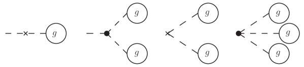
(a)

(b)

Figure 1: Graphical representations of effective Hamiltonians for (a) $\phi^{3}$ theory and (b) $\phi^{4}$ theory. The crosses represent kinetic energy terms, and the dots, interaction terms. Circles with $g$ and $\alpha$ represent zero-mode creation.

The eigenvalue problem in the valence sector, $P_{v}\overline{{\cal P}^{-}}|0\rangle=P^{-}|0\rangle$, becomes

$$\left[\frac{1}{2}4\pi\mu^{2}\int dp_{1}^{+}dp_{2}^{+}\delta(p_{1}^{+}+p_{2}^{+})g(p_{1}^{+})g(p_{2}^{+})\right.$$

$$\left.+\frac{1}{6}4\pi\lambda\int dp_{1}^{+}dp_{2}^{+}dp_{3}^{+}\delta(p_{1}^{+}+p_{2}^{+}+p_{3}^{+})g(p_{1}^{+})g(p_{2}^{+})g(p_{3}^{+})\right]|0\rangle=P^{-}|0\rangle.$$

For a function $g(p^{+})=\alpha\delta(p^{+})$, the eigenvalue $P^{-}$ is

$$P^{-}=\frac{1}{2}\mu^{2}\alpha^{2}4\pi\delta(0)+\frac{1}{6}\lambda\alpha^{3}4\pi\delta(0),$$ (14)

proportional to the volume

$$\int dx^{-}=\lim_{p^{+}\rightarrow 0}\int dx^{-}e^{ip^{+}x^{-}/2}=4\pi\delta(0).$$ (15)

We can then write $P^{-}={\cal E}^{-}\int dx^{-}$ in terms of an energy density ${\cal E}^{-}=\frac{1}{2}\mu^{2}\alpha^{2}+\frac{1}{6}\lambda\alpha^{3}$. Thus, the spectrum is unbounded from below as $\alpha$ goes to negative infinity.

The function $g$ is determined by the auxiliary equation $(1-P_{v})\overline{{\cal P}^{-}}|\phi(\underline{P})\rangle=0$, truncated to only one zero mode,

$$\sqrt{4\pi}\mu^{2}\frac{g(p^{+})}{\sqrt{p^{+}}}+\frac{1}{2}\sqrt{4\pi}\lambda\int_{0}^{p^{+}}\frac{dp^{\prime+}}{\sqrt{p^{+}}}g(p^{\prime+})g(p^{+}-p^{\prime+})=0.$$ (16)

If this is multiplied by $\sqrt{p^{+}}$, a Laplace transform $G(s)\equiv\int_{0}^{\infty}e^{-sp^{+}}g(p^{+})dp^{+}$ yields

$$\mu^{2}G(s)+\frac{1}{2}\lambda G(s)^{2}=0.$$ (17)

The solutions are $G(s)$=0 and $-2\mu^{2}/\lambda$. The inverse transform is then proportional to a delta function, and we obtain the expected $g(p^{+})=\alpha\delta(p^{+})$ with $\alpha=0$ and $\alpha=-2\mu^{2}/\lambda$. These values of $\alpha$ correspond to the local extrema of ${\cal E}^{-}$; only the global extrema at $\pm\infty$ are missed by the auxiliary equation.

With the $T$ operator truncated to one zero mode, $|\alpha\rangle\equiv\sqrt{Z_{\alpha}}e^{T}|0\rangle$ is a coherent state coherentstates . We can then minimize the vacuum energy density $\langle\alpha|{\cal H}|\alpha\rangle$ with respect to $\alpha$, given the Hamiltonian density

$${\cal H}=\frac{1}{2}\mu^{2}\phi^{2}+\frac{\lambda}{3!}\phi^{3}.$$ (18)

The $T$ operator can be written

$$T=\alpha\int_{0}^{\infty}dp^{+}\sqrt{4\pi p^{+}}\Delta(p^{+})a^{\dagger}(p^{+}),$$ (19)

where $g(p^{+})$ has been replaced by $\alpha\Delta(p^{+})$. When a specific form is needed, we take

$$\Delta(p^{+})=\frac{1}{\epsilon}e^{-p^{+}/\epsilon},$$ (20)

defined so that $\lim_{\epsilon\rightarrow 0}\Delta(p^{+})=\delta(p^{+})$ for integrals from 0 to $\infty$.

From the commutators

$${[}T^{\dagger},T] = 4\pi\alpha^{2}\int dp^{+}p^{+}\Delta^{2}(p^{+})\rightarrow\pi\alpha^{2},$$ (21)

$${[}\phi,T] = \alpha\int dp^{+}\Delta(p^{+})e^{-ip^{+}x^{-}/2}\rightarrow\alpha,$$ (22)

$${[}\phi,T^{\dagger}] = \alpha\int dp^{+}\Delta(p^{+})e^{+ip^{+}x^{-}/2}\rightarrow\alpha,$$ (23)

we have, for real $\alpha$, the normalization $\sqrt{Z_{\alpha}}=e^{-\pi\alpha^{2}/2}$, as well as $\phi|\alpha\rangle=\alpha|\alpha\rangle$, $\langle\alpha|\phi=\langle\alpha|\alpha$, and

$$\langle:\!{\cal H}\!:\rangle=\frac{1}{2}\mu^{2}\alpha^{2}+\frac{1}{6}\lambda\alpha^{3}={\cal E}^{-}.$$ (24)

The local extrema are at $\alpha=0$ and $\alpha=-2\mu^{2}/\lambda$, and the global extrema at $\pm\infty$, as in the LFCC analysis. The vacuum expectation value for the field is just $\langle\alpha|\phi|\alpha\rangle=\alpha$.

III $\phi^{4}$ theory

The Lagrangian is

$${\cal L}=\frac{1}{2}(\partial_{\mu}\phi)^{2}-\frac{1}{2}\mu^{2}\phi^{2}-\frac{\lambda}{4!}\phi^{4}.$$ (25)

We again split the light-front Hamiltonian ${\cal P}^{-}$ into two parts, with ${\cal P}_{\rm free}^{-}$ as before and

$${\cal P}_{\rm int}^{-} = \frac{\lambda}{6}\int\frac{dp_{1}^{+}dp_{2}^{+}dp_{3}^{+}}{4\pi\sqrt{p_{1}^{+}p_{2}^{+}p_{3}^{+}(p_{1}^{+}+p_{2}^{+}+p_{3}^{+})}}$$

$$\rule{72.26999pt}{0.0pt}\times\left[a^{\dagger}(p_{1}^{+}+p_{2}^{+}+p_{3}^{+})a(p_{1}^{+})a(p_{2}^{+})a(p_{3}^{+})\right.$$

$$\rule{90.3375pt}{0.0pt}\left.+a^{\dagger}(p_{1}^{+})a^{\dagger}(p_{2}^{+})a^{\dagger}(p_{3}^{+})a(p_{1}^{+}+p_{2}^{+}+p_{3}^{+})\right]$$

$$+\frac{\lambda}{4}\int\frac{dp_{1}^{+}dp_{2}^{+}}{4\pi\sqrt{p_{1}^{+}p_{2}^{+}}}\int\frac{dp_{1}^{\prime+}dp_{2}^{\prime+}}{\sqrt{p_{1}^{\prime+}p_{2}^{\prime+}}}\delta(p_{1}^{+}+p_{2}^{+}-p_{1}^{\prime+}-p_{2}^{\prime+})$$

$$\rule{144.54pt}{0.0pt}\times a^{\dagger}(p_{1}^{+})a^{\dagger}(p_{2}^{+})a(p_{1}^{\prime+})a(p_{2}^{\prime+})$$

$$+\frac{\lambda}{24}\int\frac{dp_{1}^{+}dp_{2}^{+}dp_{3}^{+}dp_{4}^{+}}{4\pi\sqrt{p_{1}^{+}p_{2}^{+}p_{3}^{+}p_{4}^{+}}}\delta(p_{1}^{+}+p_{2}^{+}+p_{3}^{+}+p_{4}^{+})$$

$$\rule{14.45377pt}{0.0pt}\times\left[a^{\dagger}(p_{1}^{+})a^{\dagger}(p_{2}^{+})a^{\dagger}(p_{3}^{+})a^{\dagger}(p_{4}^{+})+a(p_{1}^{+})a(p_{2}^{+})a(p_{3}^{+})a(p_{4}^{+})\right].$$

The $T$ operator is approximated by

$$T=\alpha\int_{0}^{\infty}dp^{+}\sqrt{4\pi p^{+}}\Delta(p^{+})a^{\dagger}(p^{+}),$$ (27)

with $\Delta(p^{+})\rightarrow\delta(p^{+})$.

The effective Hamiltonian in the vacuum sector is

$$\overline{{\cal P}^{-}} = \sqrt{4\pi}\left[\mu^{2}\alpha+\frac{1}{6}\lambda\alpha^{3}\right]\int\frac{dp^{+}}{\sqrt{p^{+}}}\Delta(p^{+})a^{\dagger}(p^{+})$$

$$+4\pi\left[\frac{1}{2}\mu^{2}\alpha^{2}+\frac{1}{24}\lambda\alpha^{4}\right]\delta(0).$$

A graphical representation is shown in Fig. 1(b).

For a vacuum valence state, the valence eigenvalue problem is

$$P_{v}\overline{{\cal P}^{-}}|0\rangle={\cal E}^{-}\int dx^{-}|0\rangle,$$ (29)

with ${\cal E}^{-}=\frac{1}{2}\mu^{2}\alpha^{2}+\frac{1}{24}\lambda\alpha^{4}$. The auxiliary equation, projected onto the one-zero-mode sector, yields

$$\mu^{2}\alpha+\frac{1}{6}\lambda\alpha^{3}=0.$$ (30)

The solutions are $\alpha=0$ or $\alpha^{2}=-6\mu^{2}/\lambda$, with $\alpha$ the vacuum expectation value for the field. A coherent-state analysis yields the same results LFCCzeromodes .

For the wrong-sign case, where $\mu^{2}\rightarrow-\mu^{2}$, the solution $\alpha=\pm\sqrt{6\lambda}/\mu$ corresponds to a shift of the field $\phi$. This shift brings the Hamiltonian density to a minimum and shows that the inclusion of a zero mode in the LFCC $T$ operator is an important step.

In general, the effective Hamiltonian will have terms that mix Fock states with odd and even numbers of particles, which is characteristic of broken symmetry. For example, a commutator that contributes to the Baker–Hausdorff expansion of $\overline{{\cal P}^{-}}$ is

$${[}{\cal P}_{\rm int}^{-},T] = \frac{\lambda\alpha}{2}\int\frac{dp_{1}^{+}dp_{2}^{+}dp^{+}}{\sqrt{4\pi p_{1}^{+}p_{2}^{+}p^{+}}}\delta(p^{+}-p_{1}^{+}-p_{2}^{+})$$

$$\rule{36.135pt}{0.0pt}\times\left[a^{\dagger}(p^{+})a(p_{1}^{+})a(p_{2}^{+})+a^{\dagger}(p_{1}^{+})a^{\dagger}(p_{2}^{+})a(p^{+})\right],$$

which changes particle number by one.

IV Summary

In light-front quantization, the vacuum is trivial without zero modes. The LFCC method, which solves the light-front Hamiltonian eigenvalue problem nonperturbatively, can be extended to include zero modes. In $\phi^{3}$ and $\phi^{4}$ theories, we have shown that this provides for the standard vacuum expectation value and is consistent with a variational coherent-state analysis. A four-zero-mode calculation in $\phi^{4}$ theory is underway, to compute the critical coupling for dynamical symmetry breaking. Another accessible application is a nonperturbative calculation of the Higgs mechanism.

References

• (1) Chabysheva SS, Hiller, JR (2012) A light-front coupled-cluster method for the nonperturbative solution of quantum field theories. Phys. Lett. B 711: 417-422
• (2) Chabysheva SS, Hiller JR (2014) Zero modes in the light-front coupled-cluster method. Ann. Phys. 340: 188-204
• (3) H.-C. Pauli H-C, Brodsky SJ (1985) Solving field theory in one space one time dimension. Phys. Rev. D 32: 1993-2000; Discretized light cone quantization: Solution to a field theory in one space one time dimensions. Phys. Rev. D 32: 2001-2013
• (4) Rozowsky JS, Thorn CB (2000) Spontaneous symmetry breaking at infinite momentum without $P^{+}$ zero modes. Phys. Rev. Lett. 85: 1614-1617
• (5) Kim VT, Pivovarov GB, Vary JP (2004) Phase transition in light-front $\phi^{4}_{1+1}$. Phys. Rev.  D 69: 085008; Chakrabarti D, Harindranath A, Martinovic L, Vary JP (2004) Kinks in discrete light cone quantization. Phys. Lett. B 582: 196-202; Chakrabarti D, Harindranath A, Martinovic L, Pivovarov GB, Vary JP (2005) Ab initio results for the broken phase of scalar light front field theory. Phys. Lett. B 617: 92-98; Chakrabarti D, Harindranath A, Vary JP (2005) A transition in the spectrum of the topological sector of $\phi^{4}_{2}$ theory at strong coupling. Phys. Rev. D 71: 125012; Martinovic L (2008) Spontaneous symmetry breaking in light front field theory. Phys. Rev. D 78: 105009
• (6) Chabysheva SS, Hiller JR (2009) Zero momentum modes in discrete light-cone quantization. Phys. Rev. D 79: 096012
• (7) Baym G (1960) Inconsistency of cubic boson-boson interactions. Phys. Rev. 117: 886-888
• (8) Swenson JB, Hiller JR (1993) Numerical signatures of vacuum instability in a one-dimensional Wick-Cutkosky model on the light cone. Phys. Rev. D 48: 1774-1780
• (9) Dirac PAM (1949) Forms of relativistic dynamics. Rev. Mod. Phys. 21: 392-399
• (10) For reviews of light-cone quantization, see Burkardt M (2002) Light front quantization. Adv. Nucl. Phys. 23: 1-74; Brodsky SJ, Pauli H-C, Pinsky SS (1998) Quantum chromodynamics and other field theories on the light cone. Phys. Rep. 301: 299-486
• (11) Harindranath A, Vary JP (1988) Variational calculation of the spectrum of $\phi^{4}$ in two-dimensions in light front field theory. Phys. Rev. D 37: 3010-3013; Misra A (1994) Coherent states in null plane QED. Phys. Rev. D 50: 4088-4096; Misra A (1996) Light cone quantization and the coherent state basis. Phys. Rev. D 53: 5874-5885; Misra A (2000) Coherent states in light front QCD. Phys. Rev. D 62: 125017; Misra A (2005) Method of asymptotic dynamics in light-front field theory. Few Body Sys. 36: 201-204; Martinovic L (1997) Non-trivial Fock vacuum of the light front Schwinger model. Phys. Lett. B 400: 335-340; Martinovic L (2006) Spontaneous symmetry breaking and Higgs mechanism in a light front formulation. Nucl. Phys. B (Proc. Suppl.) 161: 153-159; Martinovic L, Vary JP (1999) Theta-vacuum of the bosonized massive light front Schwinger model. Phys. Lett. B 459: 186-192; More JP, Misra A (2012) Infra-red divergences in light-front QED and coherent state basis. Phys. Rev. D 86: 065037; More JP, Misra A (2013) Fermion self energy correction in light-front QED using coherent state basis. Phys. Rev. D 87: 085035