E-mail: bertola@mathstat.concordia.ca, Alexander.Katsevich@ucf.edu, Alexander.Tovbis@ucf.edu

Abstract

We study the asymptotics of singular values and singular functions of a Finite Hilbert transform (FHT), which is defined on several intervals. Transforms of this kind arise in the study of the interior problem of tomography. We suggest a novel approach based on the technique of the matrix Riemann-Hilbert problem and the steepest descent method of Deift-Zhou. We obtain a family of matrix RHPs depending on the spectral parameter $\lambda$ and show that the singular values of the FHT coincide with the values of $\lambda$ for which the RHP is not solvable. Expressing the leading order solution as $\lambda\to 0$ of the RHP in terms of the Riemann Theta functions, we prove that the asymptotics of the singular values can be obtained by studying the intersections of the locus of zeroes of a certain Theta function with a straight line. This line can be calculated explicitly, and it depends on the geometry of the intervals that define the FHT. The leading order asymptotics of the singular functions and singular values are explicitly expressed in terms of the Riemann Theta functions and of the period matrix of the corresponding normalized differentials, respectively. We also obtain the error estimates for our asymptotic results.

1 Introduction

Fix any $2g+2$, $g\in{\mathbb{N}}$, distinct points $a_{i}$ on the real line $a_{i}<a_{i+1}$, $i=1,2,\dots,2g+1$. Consider the Finite Hilbert Transform (FHT)

$$({\mathcal{H}}f)(x):=\frac{1}{\pi}\int_{a_{1}}^{a_{2g+2}}\frac{f(y)}{y-x}dy,\ f\in L^{2}([a_{1},a_{2g+2}]).$$ (1.1)

Here and throughout the paper singular integrals are understood in the principal value sense. It is well-known that if $f$ is supported on $[a_{1},a_{2g+2}]$ and ${\mathcal{H}}f$ is known on $[a_{1},a_{2g+2}]$, then one can stably reconstruct $f$ using classical FHT inversion formulas [Tri57] (properties of the FHT in various $L^{p},~{}p>1,$ spaces can be found in [OE91]). In some applications, for example, in tomography, there arise problems with incomplete data, where ${\mathcal{H}}f$ is known only on a subinterval of $[a_{1},a_{2g+2}]$ (see Section 2). Since any singularity of $f$ located outside of the interval where ${\mathcal{H}}f$ is given is smoothed out and not visible from the data, we conclude that stable recovery of $f$ may be possible only on the interval where ${\mathcal{H}}f$ is known. Thus we suppose that our data are

$$({\mathcal{H}}f)(x)=\varphi(x),\ x\in[a_{2},a_{2g+1}],$$ (1.2)

and we want to find $f$ on $[a_{2},a_{2g+1}]$. Consider the operator

$${\mathcal{H}}:\,L^{2}([a_{1},a_{2g+2}])\to L^{2}([a_{2},a_{2g+1}]).$$

Unique recovery of $f$ on $[a_{2},a_{2g+1}]$ is impossible since ${\mathcal{H}}$ has a non-trivial kernel (see [KT12] for its complete description). Therefore, to achieve unique recovery the data $\varphi$ should be augmented by some additional information. One type of information that guarantees uniqueness is the knowledge of $f$ on some interval or intervals inside $[a_{2},a_{2g+1}]$. Let us assume that $f$ is known on the interior intervals

$$I_{i}:=[a_{3},a_{4}]\cup[a_{5},a_{6}]\cup\dots\cup[a_{2g-1},a_{2g}].$$ (1.3)

Denote by $I_{e}:=[a_{1},a_{2}]\cup[a_{2g+1},a_{2g+2}]$ the remaining “exterior” intervals. Applying the FHT inversion formula (see e.g. [OE91]) to $\varphi(x)=({\mathcal{H}}f)(x)\in L^{2}([a_{1},a_{2g+2}])$, we get

$$\begin{split}f(y)&=-\frac{w(y)}{\pi}\left(\int_{a_{1}}^{a_{2}}+\int_{a_{2g+1}}^{a_{2g+2}}\right)\frac{\varphi(x)}{w(x)(x-y)}dx-\frac{w(y)}{\pi}\int_{a_{2}}^{a_{2g+1}}\frac{\varphi(x)}{w(x)(x-y)}dx,\\ &{\rm where}~{}~{}a_{1}<y<a_{2g+2}~{}~{}{\rm and}~{}~{}w(x):=\sqrt{(a_{2g+2}-x)(x-a_{1})}.\end{split}$$ (1.4)

The left side of (1.4) is known on $I_{i}$. The last integral on the right is known everywhere. Combining these known quantities we get an integral equation:

$$({\mathcal{H}}^{-1}_{e}\varphi)(y):=-\frac{w(y)}{\pi}\int_{I_{e}}\frac{\varphi(x)}{w(x)(x-y)}dx=\psi(y),\ y\in I_{i},$$ (1.5)

where

$$\psi(y)=f(y)+\frac{w(y)}{\pi}\int_{a_{2}}^{a_{2g+1}}\frac{\varphi(x)}{w(x)(x-y)}dx,\ y\in I_{i},$$ (1.6)

is a known function. Here and throughout the paper the symbol $\mathcal{H}_{e}^{-1}$ denotes only the restriction of the inverse of $\mathcal{H}$ to the set $I_{e}$ but not the inverse operator itself. The problem of finding $f$ can be solved in two steps. In step 1 we solve equation (1.5) for $\varphi(x)$ on $I_{e}$. In step 2 we substitute the computed $\varphi(x)$ into (1.4) and recover $f$.

Figure 1: A schematic arrangement of the multi intervals $I_{e}$ (external) and $I_{i}$ (internal), here with $g=3$.

It is clear that solving (1.5), i.e. inverting ${\mathcal{H}}^{-1}_{e}$, is the most unstable step. The study of this step is the main motivation for this paper. We consider the operator ${\mathcal{H}}^{-1}_{e}$ in (1.5) as a map between two weighted $L^{2}$-spaces:

$${\mathcal{H}}^{-1}_{e}:\ L^{2}(I_{e},1/w)\to L^{2}(I_{i},1/w).$$ (1.7)

Then its adjoint is the Hilbert transform:

$$({\mathcal{H}}_{i}\psi)(x):=\frac{1}{\pi}\int_{I_{i}}\frac{\psi(y)}{y-x}dy,\ x\in I_{e}.$$ (1.8)

The weighted spaces for the operator ${\mathcal{H}}^{-1}_{e}$ in (1.7) are naturally determined by the structure of (1.5). In particular, as follows from inequality (1.7) of [EO04], ${\mathcal{H}}^{-1}_{e}$ is a continuous operator from $L^{2}(I_{e},1/w)$ to $L^{2}(I_{i},1/w)$, but it is not continuous from $L^{2}(I_{e})$ to $L^{2}(I_{i})$.

Our aim is to study the singular value decomposition (SVD) for the operator ${\mathcal{H}}^{-1}_{e}$. Namely, we are interested in the singular values $2\lambda=2\lambda_{n}>0$, $n\in{\mathbb{N}}$, and the corresponding left and right singular functions $f=f_{n},~{}h=h_{n}$, satisfying

$$\begin{split}({\mathcal{H}}^{-1}_{e}h)(y)=-\frac{w(y)}{\pi}&\int_{I_{e}}\frac{h(x)}{w(x)(x-y)}dx={2}\lambda f(y),\ y\in I_{i},\\ ({\mathcal{H}}_{i}f)(x)=\frac{1}{\pi}&\int_{I_{i}}\frac{f(y)}{y-x}dy={2}\lambda h(x),\ x\in I_{e}.\end{split}$$ (1.9)

Note that both integrals in (1.9) are nonsingular.

It is well known that the rate at which the $\lambda_{n}$’s approach zero is related with the ill-posedness of inverting ${\mathcal{H}}^{-1}_{e}$. Because of the symmetry $(\lambda,f,h)\Leftrightarrow(-\lambda,-f,h)$ of (1.9), we are interested only in positive $\lambda_{n}$. Thus, equation (1.9) is the main object of the present work, and obtaining the large $n$ asymptotics of $\lambda_{n}$, $f_{n}$ and $h_{n}$ is our main goal.

Our approach relies upon a reformulation of SVD problem for (1.9) in terms of a matrix Riemann Hilbert Problem (RHP) depending on a large parameter $\varkappa=-\ln\lambda$ and, subsequently, the use of the steepest descent method of Deift and Zhou for the large $\varkappa$ asymptotics of this RHP. In the last two decades, the steepest descent method for asymptotic solution of matrix RHPs has found an increasingly wide scope of applications, such as, for example: universality in random matrix theory (as the size of the matrix becomes large) and closely related asymptotic problems for large degree orthogonal polynomials; the long time and semiclassical asymptotics of integrable nonlinear equations; connection formulæ for Painlevé transcendents; approximation theory; behavior of gap-formation probabilities in certain random point processes, etc. This list can certainly be continued. A good introduction to matrix Riemann-Hilbert problems and their applications to random matrices and orthogonal polynomials can be found in the book [Dei99] of P. Deift; some more recent results and perspectives can be also found in the [BKL⁺08].

The above examples require the leading order approximate solution of an RHP in the appropriate asymptotic regime; the existence of such leading order solutions is a general feature of the above examples.

More recently, there appeared problems where the failure of solvability of the corresponding RHP was of particular interest; relevant examples include the description of the first oscillations behind the point of gradient catastrophe in the focusing nonlinear Schrödinger equation [BT13], the poles of the Painlevé transcendents (see [FIKN06] and references therein) etc.

The present paper is a further step in this general direction; the twist, however, is that our interest is now focused on the non-generic situation where our RHP is not solvable. This situation leads to the detailed study of a particular object which is known in the literature on Riemann surfaces as the “theta divisor”. Without entering into details now, the theta divisor is the locus of zeros of a particular analytic function (Riemann Theta function $\Theta$) of several variables. These variables encode the parameters of the problem we study (the points $a_{j}$, $j=1,\dots,2g+2$) as well as the spectral variable $\varkappa$. When these variables are on the theta divisor, the spectral parameter $2\lambda=2e^{-\varkappa}$ approximates a singular value of ${\mathcal{H}}^{-1}_{e}$. This is somewhat similar to the eigenvalue problem for the finite spherical well in quantum mechanics, where the zeroes of a special function (Bessel function) correspond to the eigenvalues of the problem.

In order to achieve this analysis we need to use certain properties of Theta functions, some of which can be found in Appendix A. It seems that even in the specialized literature on Theta functions we could not find the results that we need and thus a good deal of our effort goes in that direction.

Let us now return to the system (1.9). The goals of the paper are:

• to describe the asymptotics of singular values (including their multiplicity) $2\lambda_{n}$ of ${\mathcal{H}}^{-1}_{e}$;

• to describe the asymptotics of the left and right singular functions $f_{n}$ and $h_{n}$.

As it was mentioned above, we will associate the singular-value problem for ${{\mathcal{H}}^{-1}_{e}}$ with an RHP 3.10 that depends on a parameter $\lambda$ and prove that:

1. the singular values $2\lambda_{n}$ of ${{\mathcal{H}}_{e}^{-1}}$ are simple and correspond exactly to the values of $\lambda$ for which the RHP 3.10 is not solvable;

2. in the regime of small $\lambda$ the RHP 3.10 –and its non solvability– can be approximated by another ”model” RHP 4.7. The solvability of the latter depends entirely on whether a given value of the spectral parameter $\varkappa=-\ln\lambda$ will turn a certain Riemann Theta function $\Theta$ into zero, that is, whether $\varkappa$ brings the (vector) argument of $\Theta$ on the theta-divisor.

The description of our findings for the eigenfunctions would require the introduction of many notations related to Theta functions; thus, we found it expedient to refer the reader to Corollary 7.24 in Section 7. It is however possible to describe here the asymptotics of the singular values $2\lambda_{n}$ of ${{\mathcal{H}}^{-1}_{e}}$ from Theorem 7.13; namely

$$\lambda_{n}={\rm e}^{-\frac{ni\pi}{\tau_{11}}+\mathcal{O}(1)}\ ,\ \ n\to\infty,$$ (1.10)

where $\tau_{11}$ is a purely imaginary number with positive imaginary part. Specifically, it is the $(1,1)$ entry of the normalized matrix of periods ${\tau}$ associated to a double-sheeted covering of the plane, slit along the segments constituting $I_{i},I_{e}$ (i.e., a hyperelliptic surface). If we introduce a $g\times g$ matrix $\mathbb{A}$ by

$$(\mathbb{A})_{kj}=2\int_{a_{2k}}^{a_{2k+1}}\frac{z^{j-1}dz}{R(z)},~{}~{}~{}k=1,\dots,g-1~{}~{}~{}~{}{\rm and}~{}~{}~{}(\mathbb{A})_{gj}=2\int_{a_{1}}^{a_{2g+2}}\frac{z^{j-1}dz}{R_{+}(z)},~{}~{}~{}~{}j=1,\dots,g,$$ (1.11)

where $R(z)=\prod_{j=1}^{2g+2}(z-a_{j})^{\frac{1}{2}}$ is an analytic function on ${\mathbb{C}}\setminus(I_{e}\cup I_{i})$ behaving as $z^{g+1}$ at infinity, then

$${\tau}_{11}=-2\sum_{j=1}^{g}(\mathbb{A}^{-1})_{j1}\int_{I_{e}}\frac{z^{j-1}dz}{R_{+}(z)}.$$ (1.12)

Here and throughout the paper the subscripts $\pm$ routinely denote limiting values of functions (vectors, matrices) from the left/right side of corresponding oriented arcs. In particular, $R_{+}$ means the limiting value of $R$ on $I=I_{e}\cup I_{i}$ from $\Im z>0$. (The matrices $\mathbb{A},{\tau}$ are defined by equations (4.3) and (5.1) respectively.) The analysis behind (1.10) requires describing the set of zeroes of $\Theta$ (the theta-divisor) and ensuring that, as $\lambda\to 0_{+}$, the RHP 4.7 becomes unsolvable infinitely many times. Locating the values for which this happens leads to (1.10). The asymptotics (1.10) is illustrated by Figure 2, left, where the first 22 numerically simulated $\lambda_{n}$ are compared with the asymptotic formula (1.10).

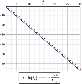
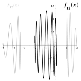
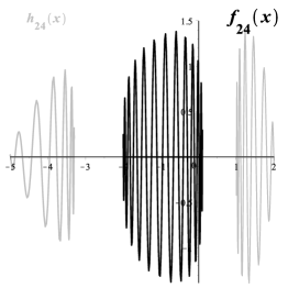
Figure 2: Plotted in the figure are $\ln(\lambda_{n})$ versus the straight line $n\mapsto-\frac{in\pi}{\tau_{11}}$ for the choice of the successive endpoints $\{-5,-3.3,-2,0.1,1,2\}$ (the case of $g=2$). The slope matches perfectly; the shift of the line is due to the $\mathcal{O}(1)$ term in (1.10). The small fluctuations of $\lambda_{n}$ away from linear behavior are explained by the periodicity of the Theta divisor and the fact that the line shown in Figure 9 has, in general, an irrational slope, so that the intersections are quasi-periodic. Observe that the log-linearity of the eigenvalues seems to be correct not only asymptotically in $n$, but even for the first singular values. Also plotted are two pairs of the corresponding singular functions $(f_{12},h_{12})$ and $(f_{24},h_{24})$, obtained numerically simultaneously with $\lambda_{n}$. Note, the envelope of the oscillations is already visibly the same, as expected from the asymptotic description in Corollary 7.24, Remark 7.23.

The outline of our paper is the following. In Section 2 we discuss practical motivations of the SVD problem (1.9) coming from tomography. In Section 3 we reformulate the SVD problem as an eigenvalue problem for an appropriate self-adjoint operator $\widehat{K}$ defined on $L^{2}(I)$. We next associate with $\widehat{K}$ a matrix RHP 3.10 in terms of which we can construct the resolvent operator $\widehat{R}$ of $\widehat{K}$ and hence, the eigenfunctions of $\widehat{K}$. We show that $2\lambda$ is a singular value of ${\mathcal{H}}^{-1}_{e}$ if and only if $\lambda$ is a positive eigenvalue of $\widehat{K}$, which is equivalent to the assertion that the corresponding RHP 3.10 does not have a solution. We also prove that the singular values $2\lambda_{n}$ of ${\mathcal{H}}^{-1}_{e}$ are simple and that the singular functions $f_{n}(z)=\sqrt{w(z)}\phi_{n}(z)\chi_{i}(z)$, $h_{n}(z)=\sqrt{w(z)}\phi_{n}(z)\chi_{e}(z)$, where $\widehat{K}\phi_{n}=\lambda_{n}\phi_{n}$ and $\chi_{i}(z),\chi_{e}(z)$ denote the characteristic functions of $I_{i},I_{e}$ respectively.

To obtain the large $n$ asymptotics of $\lambda_{n}$ we need to study the asymptotic limit as $\lambda\rightarrow 0$ of the solution $\Gamma=\Gamma(z;\lambda)$ of RHP 3.10. That is done in Section 4, where the RHP 3.10 is asymptotically reduced to the model RHP 4.7. The latter can be solved explicitly in terms of Riemann Theta functions, see Section 5, Theorem 5.7. The accuracy of replacing the RHP 3.10 by the model RHP 4.7 is evaluated in Section 6. The asymptotics (1.10) for the singular values, as well as the large $n$ asymptotics of the singular functions $f_{n},h_{n}$, see Theorem 7.15, are obtained in Section 7. Finally, some basic facts about Riemann Theta functions are provided in Appendix A.

2 Practical motivation for the problem: relationship with tomography

In 1991 Gelfand and Graev derived a formula, which gives the Hilbert transform of a function $f$ from a collection of line integrals of $f$ [GG91]. Let $f$ be sufficiently smooth and compactly supported. We start with a practically relevant 3D case. Let $D_{f}(y,\beta)$ be the collection of integrals of $f$ along lines intersecting a fixed piecewise smooth curve $\Gamma$:

$$D_{f}(y,\beta)=\int_{0}^{\infty}f(y+t\beta)dt,\ y\in\Gamma,$$ (2.1)

where $\beta$ is a unit vector. The map $f\to D_{f}$ is known as the cone-beam transform of $f$. The step of going back from $D_{f}$ to $f$, where $f$ represents the attenuation coefficient of the object being scanned, is the main mathematical principle on which a vast majority of CT scanners are based today.

Let $y(s)$ be a parametrization of $\Gamma$. We assume that $\Gamma$ does not self-intersect and is traversed in one direction as $s$ varies over some interval $I$. Pick any two values $s_{1},s_{2}\in I$, $s_{1}\not=s_{2}$. Let $\alpha$ be a unit vector along the chord $y(s_{1}),y(s_{2})$. Then one has [GG91]:

$$\frac{1}{2}\int_{s_{1}}^{s_{2}}\frac{1}{|x-y(s)|}\left.\frac{\partial}{\partial\lambda}D_{f}\left(y(\lambda),\frac{x-y(s)}{|x-y(s)|}\right)\right|_{\lambda=s}ds=\int\frac{f(x+t\alpha)}{t}dt,$$ (2.2)

where $x$ is located on the chord between $y(s_{1})$ and $y(s_{2})$. Equation (2.2) implies that knowing the cone beam transform of $f$ one can compute the Hilbert transform of $f$ on the chords of $\Gamma$. An analogous result holds in 2D as well, where the corresponding collection of line integrals of $f$ is known as the fan beam transform of $f$.

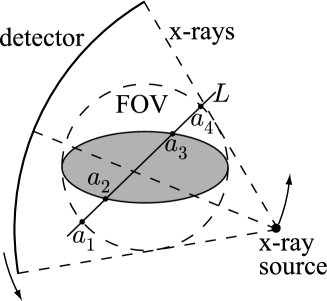
Figure 3: The geometry of the fan-beam transform.

See Figure 3, which illustrates the fan-beam transform and equation (2.2). In practice, the x-ray source and the detector are located on opposite sides of an object being scanned. The source emits multiple x-ray beams, which pass through the object and are registered by the detector. The source-detector assembly rotates around the object, and this way one collects line integral data for all lines intersecting the circular Field of View, or FOV for short (see the dashed circle in Figure 3). If the object is contained completely inside the FOV, then we know the integrals of $f$ along all lines intersecting the object (i.e., $\text{supp}\,f$). Pick any line $L$ intersecting $\text{supp}\,f$. Formula (2.2) implies that we can compute the 1D Hilbert transform of $f|_{L}$ for all points of $L$ inside the FOV, i.e. on the interval $[a_{1},a_{4}]$. Let $[a_{2},a_{3}]$ denote the support of $f|_{L}$. By assumption, $[a_{2},a_{3}]\subset[a_{1},a_{4}]$. Applying the Finite Hilbert transform inversion formula to the Hilbert data on $[a_{1},a_{4}]$, we can recover $f$ on the line. Repeating this procedure for a collection of lines $L$ that cover the support of $f$, we reconstruct all $f$.

After the importance of the Gelfand-Graev formula for image reconstruction in CT became clear in the middle 2000s, it led to a number of important advances [NCP04, DNCK06, ZPS05, YYWW07, YYW07, YYW08, KCND08, CNDK08]. In particular, new tools for investigating image reconstruction from incomplete (or, truncated) tomographic data have been developed. Suppose that instead of reconstructing all of $f$, one is interested in reconstructing only a small subset of $\text{supp}\,f$, called the Region of Interest (ROI). In this case it would be natural to reduce the x-ray exposure by blocking the x-rays that do not pass through the ROI, i.e. the FOV and ROI will coincide (see Figure 4, left panel). In the figure the reduced x-ray exposure is illustrated by a smaller detector. Now, the Hilbert transform of $f|_{L}$ is known only on $[a_{2},a_{3}]$, and $[a_{2},a_{3}]\subset\text{supp}\,f|_{L}=[a_{1},a_{4}]$.

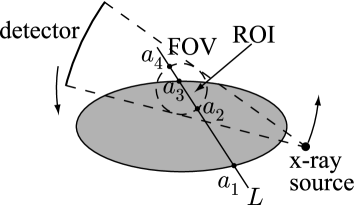
Figure 4: The interior problem (left panel) and the overlap problem (right panel).

An alternative configuration arises when a part of the FOV is outside of $\text{supp}\,f$, see Figure 4, right panel. In this case the ROI is a subset of the FOV, and $\text{supp}\,f|_{L}=[a_{1},a_{3}]$ overlaps the interval $[a_{2},a_{4}]$ where the Hilbert transform is known.

Our discussion shows that each line $L$, along which the Hilbert transform of $f$ is computed, can be considered separately from the others. Thus, we will assume in what follows that $f$ is a function of a one-dimensional argument and is defined on a line. A number of interesting results concerning the inversion of the Hilbert transform from incomplete data have been obtained. In the case of an overlap, the uniqueness and stability of computing $f$ from input data was established in [DNCK06]. Uniqueness and stability for a different configuration was established in [KCND08]. The main tool for establishing stability in [DNCK06, KCND08] was the Nevanlinna principle. In [Kat10, Kat11] a new approach for the study of the Hilbert transform with incomplete data was initiated. Let $I_{1}$ and $I_{2}$ be two intervals on the real line with distinct endpoints. All of the above problems are equivalent to solving the equation ${\mathcal{H}}f=g$ for $f$ knowing $g$, where ${\mathcal{H}}$ is the FHT that integrates over $I_{1}$ and the result is evaluated on $I_{2}$. Different relative positions of $I_{1}$ and $I_{2}$ give different problems. Hence we would like to study the operator ${\mathcal{H}}:L^{2}(I_{1})\to L^{2}(I_{2})$. The $L^{2}$ spaces are natural here because these are Hilbert spaces (i.e., it makes sense to talk about SVD), square-integrable functions is a very common class that is used in practice, and ${\mathcal{H}}:L^{2}(I_{1})\to L^{2}(I_{2})$ is continuous.

It was shown in [Kat10, Kat11] that there exists a second order linear differential operator that commutes with ${\mathcal{H}}$. This allowed the computation of the singular functions for the operator ${\mathcal{H}}$ as solutions of certain singular Sturm-Liouville problems. The cases $I_{1}\cap I_{2}=\varnothing$ and $I_{2}\subset I_{1}$ have been considered in [Kat10, Kat11]. The asymptotics of the singular functions and singular values of ${\mathcal{H}}$ in these two cases have been obtained in [KT12]. In [AAK13] the authors considered the case of an overlap, i.e. $I_{1}\cap I_{2}\not=\varnothing$, but none of the intervals is inside the other. In particular, it was shown that the spectrum of the operator ${\mathcal{H}}^{*}{\mathcal{H}}:\,L^{2}(I_{1})\to L^{2}(I_{1})$ is discrete and has two accumulation points: 0 and 1.

From the practical point of view, the interior problem illustrated in Figure 4, left panel, is most important, so we study it in more detail. Pick six points on the real axis $a_{1}<a_{2}<\dots<a_{6}$ (the reason for having two extra points will become clear shortly). Suppose that $f$ is supported on $[a_{1},a_{6}]$, and the data ${\mathcal{H}}f$ are known on a subinterval $[a_{2},a_{5}]\subset[a_{1},a_{6}]$, i.e. the equation to be solved is

$$({\mathcal{H}}f)(x)=\frac{1}{\pi}\int_{a_{1}}^{a_{6}}\frac{f(y)}{y-x}dy=\varphi(x),\ x\in[a_{2},a_{5}].$$ (2.3)

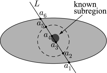
Figure 5: The interior problem with prior data. $f$ is assumed to be known inside the “known subregion”.

The goal is to recover $f$ on $[a_{2},a_{5}]$, i.e. only where the data are available. Consider ${\mathcal{H}}:\,L^{2}([a_{1},a_{6}])\to L^{2}([a_{2},a_{5}])$. As was mentioned in the previous section, this operator has a non-trivial kernel. Hence the unique recovery of $f$ on $[a_{2},a_{5}]$ is impossible. Therefore, following the suggestion of several authors [YYWW07, KCND08], we assume prior knowledge. One possibility is to assume that the 2D (or 3D) function $f$ is known on a small open set inside the ROI see Figure 5). Choosing $L$ that intersects the known subregion, we can assume that the restriction of $f$ to $L$ is known on $[a_{3},a_{4}]$ (these are the two extra points mentioned above), which leads us to the problem at the beginning of Section 1 with $g=2$. In this case the unique recovery of $f$ on $[a_{2},a_{5}]$ is theoretically possible [YYWW07, KCND08].

The assumption about prior knowledge is realistic, because quite frequently there are regions with known values of the attenuation coefficient $f$ inside the object being scanned. For instance, in medical applications of CT, $f=0$ for points inside the lungs when scanning the chest cavity of a patient. In this paper we consider a more general case $g\geq 2$, which means that there can be several intervals on $L$ where $f$ is known. Again, this is a practical assumption, since $L$ can intersect several regions inside the FOV with known $f$ (e.g., two lungs).

Theoretical analysis of the interior problem with known subregion was initiated in [CNDK08], where it was proven that finding $f$ on $(a_{2},a_{5})$ is stable in the appropriate sense. In this paper we approach the problem from a different angle. Our main task is to find the asymptotics of the singular values and singular functions of the operators ${\mathcal{H}}_{e}^{-1}$ and ${\mathcal{H}}_{i}$ (see section 1) involved in the problem. The exponential decay of the singular values in (1.10) shows that finding $\varphi$ on the exterior intervals $I_{e}:=[a_{1},a_{2}]\cup[a_{2g+1},a_{2g+2}]$ from the data is severely unstable. This, however, does not contradict the findings in [CNDK08], since the exterior intervals $I_{e}$ are not covered by the stability estimates in [CNDK08].

The most common approach to solving interior problems numerically is iterative. By their nature, iterative algorithms reconstruct $f$ both inside the ROI (i.e., on $[a_{2},a_{5}]$) and outside (i.e., on $I_{e}$). In some sense, the recovery of $f$ on $I_{e}$ means that the data $\varphi$ are recovered on $I_{e}$ as well, which is equivalent to inverting ${\mathcal{H}}_{e}^{-1}$. Hence our findings are relevant for the analysis of stability of such algorithm. Besides, we hope that in the future the results obtained in this paper will lead to novel stability estimates of the recovery of $f$ on $[a_{2},a_{5}]$.

Finally, we note that the approach to the study of the FHT with incomplete data developed in [Kat10, Kat11, KT12] does not apply since now there are six (or more) points $a_{j}$, $1\leq j\leq 2g+2$, instead of four, and there seems to be no differential operator that commutes with ${\mathcal{H}}_{e}^{-1}$ in this case. Hence a novel approach based on the matrix RHP is developed in this paper.

3 The integral operator $\hat{K}$ and the RHP

We first reformulate the SVD problem (1.9) for the operator ${\mathcal{H}}^{-1}_{e}$. It is obvious that a triple $(2\lambda,f,h)$ represents a singular value and the corresponding singular functions for the operator ${\mathcal{H}}^{-1}_{e}$ if and only if the triple $(\lambda,\widehat{f},\widehat{h})$ represents a singular value and the corresponding singular functions for the operator $H^{-1}_{e}$, where

$$\begin{split}(H^{-1}_{e}\widehat{h})(y)&:=\frac{\sqrt{w(y)}}{2\pi i}\int_{I_{e}}\frac{\widehat{h}(x)}{\sqrt{w(x)}(x-y)}dx=\lambda\widehat{f}(y),\ y\in I_{i},\\ (H_{i}\widehat{f})(x)&:=\frac{1}{2\pi i}\frac{1}{\sqrt{w(x)}}\int_{I_{i}}\frac{\widehat{f}(y)\sqrt{w(y)}}{(y-x)}dy=\lambda\widehat{h}(x),\ x\in I_{e}.\end{split}$$ (3.1)

Here $\widehat{h}=\frac{h}{\sqrt{w}}\in L^{2}(I_{e})$, $\widehat{f}=\frac{if}{\sqrt{w}}\in L^{2}(I_{i})$, and the operators $H^{-1}_{e}$, $H_{i}$ act on the corresponding unweighted $L^{2}$ spaces. It will be convenient for us to work with the system (3.1) instead of (1.9) in the remaining part of the paper.

The singular values of the system (3.1) coincide with the positive eigenvalues of the integral operator $\widehat{K}$ that will be introduced in the following Subsection 3.1. Moreover, the eigenfunctions of $\widehat{K}$ correspond to singular functions of (3.1). We also prove there that $\widehat{K}$ is a self-adjoint Hilbert–Schmidt operator with simple eigenvalues. In Subsection 3.2 we introduce a matrix RHP for $\Gamma=\Gamma(z;\lambda)$, $\lambda\neq 0$, and express the resolvent operator for $\widehat{K}$ in terms of $\Gamma$. We prove that the solution $\Gamma=\Gamma(z;\lambda)$ of this RHP exists if and only if $\lambda$ is not an eigenvalue of $\widehat{K}$. In Subsection 3.3 we express the eigenfunctions and the logarithmic derivative of the (regularized) determinant of $\widehat{K}$ in terms of $\Gamma$. These expressions will be used in Section 7 to approximate the singular functions of the system (1.9) and to prove the accuracy of the singular values in (1.10).

3.1 Definition and properties of $\widehat{K}$

Let us define the integral operator $\widehat{K}:L^{2}(I)\to L^{2}(I)$, where $L^{2}(I)=L^{2}(I_{e}\sqcup I_{i})\simeq L^{2}(I_{e})\oplus L^{2}(I_{i})$, by the requirements

$$\widehat{K}\big{|}_{L^{2}(I_{i})}=H_{i}\ ,\ \ \ \ \widehat{K}\big{|}_{L^{2}(I_{e})}=H_{e}^{-1}.$$ (3.2)

In terms of $\widehat{K}$, the SVD system (3.1) can be simply written as

$$\widehat{K}\phi=\lambda\phi,~{}~{}~{}{\rm where}~{}~{}~{}~{}\phi=\widehat{f}(z)\chi_{i}(z)+\widehat{h}(z)\chi_{e}(z)\in L^{2}(I).$$ (3.3)

Here and henceforth $\chi_{i}(z),\chi_{e}(z)$ denote the characteristic (indicator) functions of the sets $I_{i},I_{e}$, respectively. Equation (3.3) makes it clear that $(\lambda,\phi)$ is an eigenvalue/eigenfunction of $\widehat{K}$ if and only if $(\lambda,\widehat{f},\widehat{h})$ satisfies the system (3.1). We also point out that, similarly to (1.9), operator $H_{i}$ is the adjoint of $H_{e}^{-1}$.

Theorem 3.1.

The integral operator $(\hat{K}\phi)(z)=\int_{I}K(z,x)\phi(x)dx$ from $L^{2}(I)$ to $L^{2}(I)$, where

$$K(z,x)=\frac{w^{\frac{1}{2}}(x)w^{-\frac{1}{2}}(z)\chi_{e}(z)\chi_{i}(x)+w^{\frac{1}{2}}(z)w^{-\frac{1}{2}}(x)\chi_{i}(z)\chi_{e}(x)}{2i\pi(x-z)},$$ (3.4)

is a self-adjoint and a Hilbert–Schmidt operator satisfying (3.2). Moreover, the eigenvalues of $\widehat{K}$ coincide with the singular values of $H_{e}^{-1}$.

Proof.

The last statement has been established above. It is easy to check that $K(z,x)=\overline{K(x,z)}$, so that $\hat{K}$ is self-adjoint. $\hat{K}$ is also a Hilbert–Schmidt operator because

$$\int_{I\times I}|K(x,y)|^{2}dxdy=\frac{1}{2\pi^{2}}\int_{I_{i}}dx\int_{I_{e}}dy\frac{w(x)}{w(y)(x-y)^{2}}<+\infty.$$ (3.5)

Equations (3.2) follow directly from (3.4), (3.1). ∎

Remark 3.2.

Incidentally, (3.5) implies that both $H_{i},H_{e}^{-1}$ are Hilbert–Schmidt.

Corollary 3.3.

The operator $\widehat{K}$ has a real discrete set of eigenvalues $\lambda_{n},n\in{\mathbb{N}}$, that can accumulate only to $\lambda=0$.

As it was mentioned in Section 1, due to the symmetry $(\lambda,\widehat{f},\widehat{h})\leftrightarrow(-\lambda,-\widehat{f},\widehat{h})$ of the system (1.9) (and (3.1)), we can consider only nonnegative eigenvalues of $\widehat{K}$. Let $\widehat{L}=H_{e}^{-1}H_{i}:L^{2}(I_{i})\to L^{2}(I_{i})$. Thus we have immediately the following corollary.

Corollary 3.4.

$\lambda_{n}$ is an eigenvalue of $\widehat{K}$ if and only if $\lambda^{2}_{n}$ is an eigenvalue of $\widehat{L}$. Moreover, if $\phi_{n}=\widehat{f}_{n}\chi_{i}+\widehat{h}_{n}\chi_{e}$ is an eigenfunction of $\widehat{K}$ with eigenvalue $\lambda_{n}$, then $\widehat{f}_{n}$ is an eigenfunction of $\widehat{L}$ corresponding to $\lambda_{n}^{2}$.

Direct calculations show that $(\widehat{L}f)(x)=\int_{I_{i}}L(x,y)f(y)dy$, where the kernel is given by

$$L(x,y)=\frac{\sqrt{w(x)w(y)}}{4\pi^{2}}\int_{I_{e}}\frac{dz}{w(z)}\frac{1}{(z-x)(z-y)}.$$ (3.6)

Aiming now at analyzing the spectrum of $\widehat{L}$ we point out that $\widehat{L}$ is strictly Totally Positive, according to the definition below.

Definition 3.5.

An integral operator $\widehat{L}:L^{2}(I)\to L^{2}(I)$ with a continuous kernel $L(x,y)$, where $I\subset{\mathbb{R}}$ is a finite union of segments, is called strictly totally positive (sTP) if for any $n\in{\mathbb{N}}$, and for any choices of a pair of ordered $n$-tuples $x_{1}<x_{2}<\dots<x_{n},\ y_{1}<y_{2}<\dots<y_{n}$ in $I$

$$\det\left[L(x_{\ell},y_{k})\right]_{1\leq\ell,k\leq n}>0.$$ (3.7)

Lemma 3.6.

The operator $\widehat{L}=H_{e}^{-1}H_{i}$ is strictly totally positive.

Proof.

The proof is a straightforward computation using Andreief’s identity that relates determinants of single integrals and multiple integrals of determinants [And83]

$$\begin{split}\det&\left[L(x_{\ell},y_{k})\right]_{1\leq\ell,k\leq n}\\ &=\prod_{s=1}^{n}\sqrt{w(x_{s})w(y_{s})}\det\left[\int_{I_{e}}\frac{{\rm d}z}{w(z)}\frac{1}{(z-x_{\ell})(z-y_{k})}\right]_{1\leq\ell,k\leq n}\\ &\mathop{=}^{\hbox{\tiny Andreief}}\frac{\prod_{s=1}^{n}\sqrt{w(x_{s})w(y_{s})}}{n!}\int_{(I_{e})^{n}}\prod_{r=1}^{n}\frac{{\rm d}z_{r}}{w(z_{r})}\det\left[\frac{1}{z_{s}-x_{\ell}}\right]_{\ell,s\leq n}\det\left[\frac{1}{z_{s}-y_{k}}\right]_{s,k\leq n}\\ &\mathop{=}^{\text{\tiny Cauchy det}}\frac{\Delta(x)\Delta(y)\prod_{s=1}^{n}\sqrt{w(x_{s})w(y_{s})}}{n!}\int_{(I_{e})^{n}}\prod_{r=1}^{n}\frac{{\rm d}z_{r}}{w(z_{r})}\frac{[\Delta(z)]^{2}}{\prod_{\ell,s}(z_{s}-x_{\ell})\prod_{r,k}(z_{r}-y_{k})}\\ &=\frac{\Delta(x)\Delta(y)\prod_{s=1}^{n}\sqrt{w(x_{s})w(y_{s})}}{n!}\int_{(I_{e})^{n}}\prod_{r=1}^{n}\frac{{\rm d}z_{r}}{w(z_{r})}\frac{[\Delta(z)]^{2}}{\prod_{\ell,s}(z_{s}-x_{\ell})(z_{s}-y_{\ell})}.\end{split}$$ (3.8)

Here $\Delta(x)=\prod_{i<j}(x_{i}-x_{j})$ is the Vandermonde determinant. Now it is apparent that the integrand of the last expression here above is strictly positive for any $x_{j},y_{j}\in I_{i}$ and $z_{r}\in I_{e}$ because the interval $I_{i}$ is inside the external one. ∎

Theorem 3.7.

The integral operator $\widehat{L}=H_{e}^{-1}H_{i}$ has simple, positive eigenvalues.

This theorem was, in fact, proved in Kellogg [Kel18] and can also be found in [Pin96]. The only difference is that [Kel18, Pin96] consider a kernel on $L^{2}([0,1])$, whereas we have a union of disjoint intervals. However the arguments used in their proof apply verbatim. We highlight some details in Appendix B.

Corollary 3.8.

The eigenvalues of the integral operator $\widehat{K}$ are simple.

Proof.

Indeed, $\widehat{K}$ is Hilbert-Schmidt and self-adjoint and, therefore, it has a complete basis of eigenfunctions. If an eigenvalue $\lambda_{n}$ of $\widehat{K}$ is not simple, then there are at least two linearly independent eigenfunctions of $\widehat{K}$ corresponding to $\lambda_{n}$. Then, according to (3.3), $\lambda^{2}_{n}$ is not a simple eigenvalue of $\widehat{L}$. The obtained contradiction with Theorem 3.7 completes the proof. ∎

Remark 3.9.

It is also known ([Pin96]) that the $n$-th eigenfunction $\widehat{f}_{n}$ of $\widehat{L}$ corresponding to the ordered eigenvalues $\lambda_{0}^{2}>\lambda_{1}^{2}>\dots>0$ changes sign $n$ times within $I_{i}$ (and that the zeroes in the interior of $I_{i}$ are simple), see Figure 2. It will be shown in Remark 7.23 that the approximation of $\widehat{f}_{n}$ we are going to obtain is asymptotically consistent with this property.

3.2 Resolvent of $\widehat{K}$ and the Riemann–Hilbert problem

The operator $\widehat{K}$ falls within the class of “integrable kernels” [IIKS90] (see also the introduction of [BC11]) and it is known that its spectral properties are intimately related to a suitable Riemann–Hilbert problem. In particular, the kernel of the resolvent integral operator $\widehat{R}=\widehat{R}(\lambda):L^{2}(I)\to L^{2}(I)$, defined by

$$(\mathrm{Id}+\widehat{R})(\mathrm{Id}-\frac{1}{\lambda}\widehat{K})=\mathrm{Id},$$ (3.9)

can be expressed through the solution $\Gamma$ of the following RHP (as explained in Lemma 3.16 below).

Riemann-Hilbert Problem 3.10.

Find a $2\times 2$ matrix-function $\Gamma=\Gamma(z;\lambda)$, $\lambda\in{\mathbb{C}}\setminus\{0\}$, which is analytic in $\overline{{\mathbb{C}}}\setminus I$, where $I=I_{i}\cup I_{e}$, admits non-tangential boundary values from the upper/lower half-planes that belong to $L^{2}_{loc}$ in the interior points of $I$, and satisfies

$$\Gamma_{+}(z;\lambda)=\Gamma_{-}(z;\lambda)\left[\begin{matrix}1&0\\ \frac{iw}{\lambda}&1\end{matrix}\right],\ \ z\in I_{i};\qquad\Gamma_{+}(z;\lambda)=\Gamma_{-}(z;\lambda)\left[\begin{matrix}1&-\frac{i}{\lambda w}\\ 0&1\end{matrix}\right],\ \ z\in I_{e},$$ (3.10)

$$\Gamma(z;\lambda)={\bf 1}+O(z^{-1})~{}~{}~{}~{}{\rm as}~{}~{}z\rightarrow\infty,$$ (3.11)

$$\Gamma(z;\lambda)=\left[\mathcal{O}(1),\mathcal{O}((z-a_{j})^{-\frac{1}{2}})\right],~{}~{}z\rightarrow a_{j},~{}~{}j=1,2g+2,$$ (3.12)

$$\Gamma(z;\lambda)=\left[\mathcal{O}(1),\mathcal{O}(\ln(z-a_{j}))\right],~{}~{}~{}~{}z\rightarrow a_{j},~{}~{}j=2,2g+1,$$ (3.13)

$$\Gamma(z;\lambda)=\left[\mathcal{O}(\ln(z-a_{j})),\mathcal{O}(1)\right],~{}~{}~{}~{}~{}z\rightarrow a_{j},~{}~{}j=3,\dots,2g.$$ (3.14)

Here the endpoint behavior of $\Gamma$ is described column-wise. We will frequently omit the dependence on $\lambda$ from notation for convenience.

We will refer informally to the conditions (3.10), as well as similar conditions to be introduced later, as “jumps”.

Remark 3.11.

Since the jump matrices in RHP 3.10 are analytic at all points in the interior of $I$, the solution of the RHP can be easily shown to admit analytic boundary values. A similar observation applies to all the subsequent RHPs.

Proposition 3.12.

If a solution to the RHP 3.10 exists, then it is unique.

Proof.

Let $\Gamma_{1,2}$ be two solutions of the RHP 3.10. Then it is promptly seen that $(\Gamma_{2}\Gamma_{1}^{-1})(z)$ has no jumps on $I_{i},I_{e}$. If $\Gamma(z)$ satisfies RHP 3.10, $\det\Gamma$ is analytic and single-valued in $\bar{\mathbb{C}}\setminus\{a_{1},a_{2},\dots,a_{2g+2}\}$ and $\det\Gamma(\infty)=1$. Then, in view of the endpoint behavior (3.12)-(3.14), we conclude that $\det\Gamma\equiv 1$. Thus, since $\det\Gamma_{1,2}\equiv 1$, the matrix $\Gamma_{2}\Gamma_{1}^{-1}$ has no more than logarithmic growth at $a_{j}$, $j=2,\dots,2g+1$. Since only the first row of $\Gamma_{1}^{-1}(z)$ has $O((z-a_{j})^{-\frac{1}{2}})$ behavior near $a_{j},~{}j=1,2g+2,$ we conclude that $\Gamma_{2}\Gamma_{1}^{-1}=O((z-a_{j})^{-\frac{1}{2}})$ near $a_{j},~{}j=1,2g+2,$. Thus, $\Gamma_{2}(z)\Gamma_{1}^{-1}(z)$ is analytic in $\bar{\mathbb{C}}$ and approaches ${\bf 1}$ as $z\rightarrow\infty$. So, by Liouville’s theorem, $\Gamma_{2}(z)\equiv\Gamma_{1}(z)$. ∎

For convenience of matrix calculations below, throughout the paper we use the Pauli matrices

$${\sigma}_{1}=\begin{bmatrix}0&1\\ 1&0\end{bmatrix},~{}~{}~{}{\sigma}_{2}=\begin{bmatrix}0&-i\\ i&0\end{bmatrix},~{}~{}~{}{\sigma}_{3}=\begin{bmatrix}1&0\\ 0&-1\end{bmatrix}.$$

Remarks 3.13, 3.14 below follow from Proposition 3.12.

Remark 3.13.

For any $\lambda\in{\mathbb{C}}$ the solution $\Gamma(z;\lambda)$ enjoys the Schwarz symmetry

$$\overline{\Gamma(\overline{z};\overline{\lambda})}=\Gamma(z;\lambda)$$ (3.15)

because (as the reader may verify) the matrix $\overline{\Gamma(\overline{z};\overline{\lambda})}$ solves the same RHP.

Remark 3.14.

The function $\Gamma(z;\lambda)$ has the symmetry

$$\Gamma(z;-\lambda)={\sigma}_{3}\Gamma(z;\lambda){\sigma}_{3},$$ (3.16)

which follows by noticing that the jumps have the same symmetry. In particular the RHP for $\Gamma(z;\lambda)$ is solvable if and only if the one for $\Gamma(z;-\lambda)$ is. This is a reflection of the symmetry of the spectrum of the problem.

Remark 3.15.

If $\Gamma(z;\lambda)=[\vec{A}(z),\vec{B}(z)]$, where $\vec{A},\vec{B}$ are the columns of $\Gamma$, is the solution of the RHP 3.10, then $A(z)$ is analytic on $I_{e}$, and $B(z)$ is analytic on $I_{i}$. Moreover, in terms of $\vec{A},\vec{B}$, the jump and normalization conditions (3.10) and (3.11), respectively, can be written as a system

$$\begin{split}\vec{A}(z)=\left[\begin{array}[]{c}1\\ 0\end{array}\right]+\frac{1}{2\pi\lambda}\int_{I_{i}}\frac{\vec{B}(\zeta)w(\zeta)d\zeta}{\zeta-z},\ z\not\in I_{i},\\ \vec{B}(z)=\left[\begin{array}[]{c}0\\ 1\end{array}\right]-\frac{1}{2\pi\lambda}\int_{I_{e}}\frac{\vec{A}(\zeta)d\zeta}{w(\zeta)(\zeta-z)},\ z\not\in I_{e}.\end{split}$$ (3.17)

On the other hand, the system of integral equations (3.17) is equivalent to the RHP 3.10. Indeed, the jump (3.10) and normalization condition (3.11) immediately follow from (3.17). As solutions of (3.17), $\vec{A}(z)$ is analytic in $\bar{\mathbb{C}}\setminus I_{i}$ and $\vec{B}(z)$ is analytic in $\bar{\mathbb{C}}\setminus I_{e}$. Then the endpoint behavior (3.12)-(3.14) follow from properties of Cauchy operators, see [Gak66], Section 8.3.

Lemma 3.16 below is a particular case of the resolvent formula derived in [IIKS90]. In the interest of self-containedness, we present it with a proof.

Lemma 3.16.

If $\lambda$ is such that the solution $\Gamma(z;\lambda)$ of the RHP 3.10 exists, then the kernel $R$ of the resolvent $\widehat{R}$ defined by (3.9) is given by

$$R(z,x;\lambda)=\frac{\vec{g}^{t}(x)\Gamma^{-1}(x;\lambda)\Gamma(z;\lambda)\vec{f}(z)}{2i\pi\lambda(z-x)},$$ (3.18)

$$\vec{f}(z):=\left[\begin{matrix}{\frac{i\chi_{e}(z)}{\sqrt{w(z)}}}\\ \sqrt{w(z)}\chi_{i}(z)\end{matrix}\right],\ \vec{g}(x):=\left[\begin{matrix}-i\sqrt{w(x)}\chi_{i}(x)\\ \frac{\chi_{e}(x)}{\sqrt{w(x)}}\end{matrix}\right],$$ (3.19)

where $\vec{g}^{t}$ denotes the transposition of $\vec{g}$.

Proof.

The jumps of the RHP 3.10 can be written in the form

$$\Gamma_{+}(z;\lambda)=\Gamma_{-}(z;\lambda)\left({\bf 1}-\frac{1}{\lambda}\vec{f}(z)\vec{g}^{t}(z)\right),\ z\in I\ ,$$ (3.20)

and equations (3.17) can be written compactly as

$$\Gamma(z;\lambda)={\bf 1}-\int_{I}\frac{\Gamma_{-}(\zeta;\lambda)\vec{f}(\zeta)\vec{g}^{t}(\zeta)d\zeta}{2i\pi\lambda(\zeta-z)}.$$ (3.21)

Note that

$$K(z,x)=\frac{\vec{f}^{t}(z)\vec{g}(x)}{2\pi i(z-x)}~{}~{}~{}{\rm and}~{}~{}~{}\vec{f}^{t}(z)\vec{g}(z)\equiv 0,\ z\in I.$$ (3.22)

The latter equation implies that the boundary value in the integrand of (3.21) is irrelevant because $\Gamma_{+}(\zeta;\lambda)\vec{f}(\zeta)\vec{g}^{t}(\zeta)=\Gamma_{-}(\zeta;\lambda)\left({\bf 1}-\frac{\vec{f}(\zeta)\vec{g}^{t}(\zeta)}{\lambda}\right)\vec{f}(\zeta)\vec{g}^{t}(\zeta)=\Gamma_{-}(\zeta;\lambda)\vec{f}(\zeta)\vec{g}^{t}(\zeta)$.

Equation (3.9) can be written as

$$\widehat{K}\widehat{R}=\lambda\widehat{R}-\widehat{K}.$$ (3.23)

To complete the proof, it is sufficient to show that the kernel of $\widehat{K}\widehat{R}$ is equal to $\lambda R(x,y;\lambda)-K(x,y)$, where $K,R$ are given by (3.18), (3.4) respectively. Indeed, taking into account (3.22) and (3.21), we calculate the kernel of $\widehat{K}\widehat{R}$ as

$$\int_{I}d\zeta\frac{\vec{g}^{t}(y)\Gamma^{-1}(y;\lambda)\Gamma(\zeta;\lambda)\vec{f}(\zeta)}{2i\pi\lambda(\zeta-y)}\frac{\vec{g}^{t}(\zeta)\vec{f}(x)}{2i\pi(x-\zeta)}=$$ (3.24)

$$=\int_{I}d\zeta\frac{\vec{g}^{t}(y)\Gamma^{-1}(y;\lambda)\Gamma(\zeta;\lambda)\vec{f}(\zeta)\vec{g}^{t}(\zeta)\vec{f}(x)}{(2i\pi)^{2}\lambda(x-y)}\left[\frac{1}{\zeta-y}-\frac{1}{\zeta-x}\right]$$ (3.25)

$$=\frac{\vec{g}^{t}(y)\Gamma^{-1}(y;\lambda)\left(\Gamma(x;\lambda)-\Gamma(y;\lambda)\right)\vec{f}(x)}{2i\pi(x-y)}=\lambda R(x,y;\lambda)-K(x,y).$$

The conditions (3.12)-(3.14) guarantee that the integrals above are well defined. ∎

Theorem 3.17.

$\lambda\in{\mathbb{C}}\setminus\{0\}$ is an eigenvalue of $\widehat{K}$ if and only if the RHP 3.10 for $\Gamma(z;\lambda)$ has no solution.

Proof.

Suppose $\lambda$ is an eigenvalue and the RHP 3.10 has a solution. Then, according to Lemma 3.16, $\mathrm{Id}-\frac{1}{\lambda}\widehat{K}$ is invertible and this is a contradiction. Let us now assume that $\lambda$ is not an eigenvalue. Using (3.1), the system of integral equations (3.17) for columns of $\Gamma$ can be equivalently written as

$$\vec{B}(z)=\left[\begin{array}[]{c}\frac{-i}{\lambda\sqrt{w}}H^{-1}_{e}(1/\sqrt{w})\\ 1\end{array}\right]+\frac{1}{\lambda^{2}\sqrt{w}}H^{-1}_{e}H_{i}(\sqrt{w}{\vec{B}}),\ z\in I_{i}$$ (3.26)

or

$$\left(\mathrm{Id}-\frac{1}{\lambda^{2}}\frac{1}{\sqrt{w}}\circ\widehat{L}\circ\sqrt{w}\right)\vec{B}=\left[\begin{array}[]{c}\frac{-i}{\lambda\sqrt{w}}H^{-1}_{e}(1/\sqrt{w})\\ 1\end{array}\right],$$ (3.27)

where $\frac{1}{\sqrt{w}}\circ\widehat{L}\circ\sqrt{w}$ is a conjugation of $\widehat{L}$ by the multiplication operator $\sqrt{w}$ and the kernel of $\widehat{L}$ is given by (3.6). Note that this multiplication operator and its inverse are bounded (on $L^{2}(I_{i})$). According to Corollary 3.4, equation (3.27) has a solution $\vec{B}(z)\in L^{2}(I_{i})$, since $\lambda$ is not an eigenvalue of $\widehat{K}$. Then $A(z)$, given by (3.17), is analytic when $z\not\in I_{i}$, and the second equation in (3.17) holds. Thus, $\Gamma(z)=[A(z),B(z)]$ is analytic when $z\not\in I$ and satisfies the jump conditions (3.10) and the normalization (3.11). Direct calculations show that $\Gamma(z)=[A(z),B(z)]$ also satisfies endpoint behavior (3.12)-(3.14). Thus, $\Gamma(z)=\Gamma(z;\lambda)$ satisfies RHP 3.10. ∎

3.3 Eigenfunctions and further properties of $\hat{K}$

According to the spectral theorem, the resolvent $\hat{R}(\lambda)$ of $\hat{K}$ is analytic in ${\mathbb{C}}\setminus{\rm spec}(\widehat{K})$ and

$$\mathrm{Id}+\hat{R}(\lambda)=\left(\mathrm{Id}-\frac{1}{\lambda}\widehat{K}\right)^{-1}=\sum_{n}\frac{1}{1-\frac{\lambda_{n}}{\lambda}}P_{n},$$ (3.28)

where the summation runs over all the eigenvalues of $\hat{K}$, and $P_{n}$ denotes the (orthogonal) projector on the $n$-th eigenspace. Note that, according to Corollary 3.8, $\hat{R}(\lambda)$ has simple poles at the eigenvalues $\lambda_{n}$. We restrict the top equation in (3.17) to $I_{e}$ and divide it by $\sqrt{w(z)}$, while we restrict the bottom one to $I_{i}$ and multiply by $i\sqrt{w(z)}$ so that, after a rearrangement of terms, we obtain

$$\frac{\chi_{e}}{\sqrt{w(z)}}\vec{A}(z)+i\sqrt{w(z)}\chi_{i}\vec{B}(z)-$$ (3.29)

$$-\frac{\chi_{e}}{\sqrt{w(z)}} \ \ \frac{1}{2i\pi\lambda}\int_{I_{i}}\frac{i\vec{B}(\zeta)w(\zeta)d\zeta}{\zeta-z}-\frac{\chi_{i}\sqrt{w(z)}}{2i\pi\lambda}\int_{I_{e}}\frac{\vec{A}(\zeta)d\zeta}{w(\zeta)(\zeta-z)}=\left[\frac{\chi_{e}}{\sqrt{w}}\atop i\sqrt{w}\chi_{i}\right].$$

We can read (3.29) component-wise for the two functions $\varphi_{1,2}\in L^{2}(I)$ defined hereafter (restoring the notation $\Gamma_{ji}$ for the entries of $\Gamma=(\vec{A},\vec{B})$)

$$\varphi_{j}(z;\lambda)=\frac{\Gamma_{j1}(z;\lambda)}{\sqrt{w(z)}}\chi_{e}(z)+{i}{\Gamma_{j2}(z;\lambda)}{\sqrt{w(z)}}\chi_{i}(z)\in L^{2}(I_{i}\sqcup I_{e}),~{}~{}j=1,2.$$ (3.30)

Then, according to Theorem 3.1, equation (3.29) can be written as

$$\left(\mathrm{Id}-\frac{1}{\lambda}\widehat{K}\right)\varphi_{1}(z;\lambda)=\frac{\chi_{e}(z)}{\sqrt{w(z)}}\ ,\ \ \left(\mathrm{Id}-\frac{1}{\lambda}\widehat{K}\right)\varphi_{2}(z;\lambda)=i{\chi_{i}(z)}{\sqrt{w(z)}}.$$ (3.31)

Clearly, both functions exist for $\lambda\not\in{\rm spec}(\widehat{K})$ and are given by

$$\varphi_{1}(z;\lambda)=(\mathrm{Id}+\widehat{R})\frac{\chi_{e}(z)}{\sqrt{w(z)}},~{}~{}~{}\varphi_{2}(z;\lambda)=(\mathrm{Id}+\widehat{R})i{\chi_{i}(z)}{\sqrt{w(z)}}.$$ (3.32)

Moreover, they are analytic functions in $\lambda\in{\mathbb{C}}\setminus{\rm spec}(\widehat{K})$ (with values in $L^{2}(I)$) and have no more than simple poles at the eigenvalues $\lambda_{n}$ because $\widehat{R}(\lambda)$ is analytic in $\lambda$ and has simple poles by (3.28).

Vice versa, if $\varphi_{1,2}$ are solutions of (3.31) for some fixed $\lambda$, they define $\Gamma_{j1}$ on $I_{e}$ and $\Gamma_{j2}$ on $I_{i}$ through (3.30). Inserting these values into the right sides of the corresponding two equations in (3.17), we can reconstruct solution $\Gamma(z;\lambda)$ of the RHP 3.10 for all $z\in\bar{\mathbb{C}}\setminus I$. Thus we have proved the following corollary.

Corollary 3.18.

Let us fix some $\lambda\in{\mathbb{C}}\setminus\{0\}$. The solution $\Gamma(z;\lambda)$ of the RHP 3.10 exists if and only if both equations (3.31) simultaneously have a solution.

Proposition 3.19.

If $\lambda_{n}$ is an eigenvalue of $\widehat{K}$, then the functions $\phi_{n,j}(z)=\mathop{\mathrm{res}}\limits_{\lambda=\lambda_{n}}\frac{\varphi_{j}(z;\lambda)}{\lambda},j=1,2,$ are proportional to each other and satisfy $\widehat{K}\phi_{n,j}=\lambda_{n}\phi_{n,j}$. Moreover,

$$\phi_{n,j}(z)=\frac{\chi_{e}(z)}{\sqrt{w(z)}}\mathop{\mathrm{res}}\limits_{\lambda=\lambda_{n}}\Gamma_{j1}(z;\lambda)\frac{1}{\lambda}+{i}\sqrt{w(z)}\chi_{i}(z)\mathop{\mathrm{res}}\limits_{\lambda=\lambda_{n}}\Gamma_{j2}(z;\lambda)\frac{1}{\lambda},$$ (3.33)

where at least one of $\phi_{n,j}$ is not identical zero on $I$.

Proof.

Consider $j=1$, with $j=2$ being treated similarly. According to (3.31) and (3.28), we have

$$\varphi_{1}(z;\lambda)=\sum_{n}\frac{\lambda}{\lambda-{\lambda_{n}}}P_{n}(\frac{\chi_{e}}{\sqrt{w}}),~{}~{}~{}\text{so that}~{}~{}~{}\phi_{n,1}(z)=P_{n}(\frac{\chi_{e}}{\sqrt{w}}).$$ (3.34)

According to Corollary 3.8, the eigenspace of $\widehat{K}$ corresponding to $\lambda_{n}$ is one-dimensional, so that $\phi_{n,j}(z)$, $j=1,2$, is either a corresponding eigenfunction or identical zero. Therefore, $\phi_{n,j}(z)$ are proportional to each other. Equation (3.33) follows from (3.30). To prove the last statement recall that the poles of $\varphi_{j}(z;\lambda)$ at $\lambda=\lambda_{n}$ can be at most simple. If their residue is zero then both $\varphi_{j}(z;\lambda)$ must be analytic at $\lambda_{n}$. But then, according to Corollary 3.18, there exists solution $\Gamma(z;\lambda_{n})$ to the RHP 3.10 with $\lambda=\lambda_{n}$. The obtained contradiction with Theorem 3.17 completes the proof. ∎

We shall use Proposition 3.19 to extract the approximation of the eigenfunctions from the approximation of $\Gamma$, obtained in Section 5.

Let us introduce

$$t_{2}(\lambda)=\prod_{n}\left(1-\frac{\lambda_{n}}{\lambda}\right){\rm e}^{\lambda_{n}/\lambda}$$ (3.35)

where the product is taken over all the eigenvalues of $\widehat{K}$. Since $\widehat{K}$ is a Hilbert–Schmidt operator, it is straightforward to show that the product is absolutely convergent for any $\lambda\in{\mathbb{C}}$ and that $t_{2}(\lambda)$ vanishes if and only if $\lambda=\lambda_{n}$, i.e., $\mathrm{Id}-\lambda^{-1}\widehat{K}$ is not invertible. In fact, $t_{2}(\lambda)$ is known as (Carleman) regularized determinant (see [Sim05], Ch. 3) of the Hilbert–Schmidt operator $\widehat{K}$ that is denoted $t_{2}(\lambda)=\det_{2}\left(\mathrm{Id}-\frac{1}{\lambda}\widehat{K}\right)$.

Our aim now is to calculate the logarithmic derivative $\partial_{\lambda}\ln t_{2}(\lambda)$ in terms of $\Gamma$, which then allows to find $n_{\mathcal{C}}$ – the number of eigenvalues lying within a closed contour $\mathcal{C}$ in the $\lambda$-plane – by $n_{\mathcal{C}}=\frac{1}{2i\pi}\oint_{\mathcal{C}}\partial_{\lambda}\ln{t_{2}}(\lambda)d\lambda.$ This expression will allow us to localize the eigenvalues of $\widehat{K}$ using the approximation of $\Gamma$, obtained in Section 5. We see by elementary calculus that

$$\partial\ln t_{2}(\lambda)=\frac{1}{\lambda^{2}}\sum_{n}\left(\frac{\lambda_{n}}{1-\frac{\lambda_{n}}{\lambda}}-{\lambda_{n}}\right)=\frac{1}{\lambda^{2}}\mathrm{Tr}(\widehat{K}\widehat{R}),$$ (3.36)

where ${\rm Tr}\,\widehat{F}=\int_{I}F(x,x)dx$ denotes the trace of a trace-class integral operator $\widehat{F}:L^{2}(I)\rightarrow L^{2}(I)$ with the kernel $F(x,y)$ (see e.g. [Sim05]). Indeed, observe that: i) the series in (3.36) is absolutely convergent; ii) the operator $\widehat{R}\widehat{K}$ is of the trace class since both $\widehat{K},\widehat{R}$ are Hilbert–Schmidt operators, and; iii) the series in (3.36) is the sum of all the eigenvalues of the trace class operator $\lambda\widehat{R}-\widehat{K}=\widehat{R}\widehat{K}$, see (3.23). The following proposition expresses $\mathrm{Tr}(\widehat{K}\widehat{R})$ through the matrix $\Gamma$.

Proposition 3.20.

Let $\widehat{K}$ be the integral operator defined in Theorem 3.1, $t_{2}(\lambda)$ be its (regularized) determinant, see (3.35), and $\Gamma(z;\lambda)$ satisfies the RHP 3.10. Then

$$\partial_{\lambda}\ln t_{2}(\lambda)=-\frac{1}{\lambda i\pi}\oint_{\hat{I}_{i}}\left(\Gamma_{21}\Gamma_{12}^{\prime}-\Gamma_{11}\Gamma_{22}^{\prime}\right)dz,$$ (3.37)

where $\hat{I}_{i}$ is a clockwise loop surrounding $I_{i}$, $\Gamma_{jk}$’s are the entries of $\Gamma$, and prime denotes the derivative with respect to $z$.

Proof.

Expressing the kernel of $\widehat{R}\widehat{K}$ through $R,K$, see (3.18), (3.22), we calculate the right hand side of (3.36) as

$$\begin{split}\mathrm{Tr}\left(\widehat{K}\widehat{R}\right)=&\int_{I}dx\int_{I}d\zeta\frac{\vec{g}^{t}(x)\Gamma^{-1}(x;\lambda)\Gamma(\zeta;\lambda)\vec{f}(\zeta)}{2i\pi\lambda(\zeta-x)}\frac{\vec{g}^{t}(\zeta)\vec{f}(x)}{2i\pi(x-\zeta)}\\ =&\int_{I_{e}}\frac{-dx}{2\pi w(x)}\int_{I}d\zeta\frac{(\Gamma^{-1}(x;\lambda)\Gamma(\zeta;\lambda)\vec{f}(\zeta)\vec{g}^{t}(\zeta))_{21}}{2i\pi\lambda(\zeta-x)^{2}}\\ &\qquad+\int_{I_{i}}\frac{w(x)dx}{2\pi}\int_{I}d\zeta\frac{\big{(}\Gamma^{-1}(x;\lambda)\Gamma(\zeta;\lambda)\vec{f}(\zeta)\vec{g}^{t}(\zeta)\big{)}_{12}}{2i\pi\lambda(\zeta-x)^{2}}.\end{split}$$ (3.38)

Note that $\vec{f}(z)\vec{g}^{t}(z)=\left[\begin{array}[]{cc}0&\frac{i\chi_{e}(z)}{w(z)}\\ {-i}\chi_{i}(z){w(z)}&0\end{array}\right]$ and, therefore, the first integral over $I$ in (3.38) can be replaced by the same integral over $I_{i}$, whereas the second integral over $I$ can be replaced by the same integral over $I_{e}$. Thus, both integrals in (3.38) are nonsingular.

Considering the $j,k$ entry of differentiated equation (3.21), we obtain

$$\Gamma^{\prime}_{jk}(z;\lambda)=-\int_{I}d\zeta\frac{\big{(}\Gamma(\zeta;\lambda)\vec{f}(\zeta)\vec{g}^{t}(\zeta)\big{)}_{jk}}{2i\pi\lambda(\zeta-z)^{2}}$$ (3.39)

provided that the integral is well defined. But this is exactly the case in (3.38) where the integrals are nonsingular. Thus, (3.38) and (3.39) imply

$$\begin{split}\partial_{\lambda}\ln t_{2}(\lambda)&=\int_{I_{e}}\frac{dx}{2\pi\lambda^{2}w(x)}\left(\Gamma^{-1}(x;\lambda)\Gamma^{\prime}(x;\lambda)\right)_{21}-\int_{I_{i}}\frac{w(x)dx}{2\pi\lambda^{2}}\left(\Gamma^{-1}(x;\lambda)\Gamma^{\prime}(x;\lambda)\right)_{12}\\ =-\frac{1}{\lambda}\frac{1}{2i\pi}&\int_{I_{i}}\frac{iw(z)}{\lambda}\left(\Gamma_{22}\Gamma_{12}^{\prime}-\Gamma_{12}\Gamma_{22}^{\prime}\right)dz-\frac{1}{\lambda}\frac{1}{2i\pi}\int_{I_{e}}\frac{1}{\lambda iw(z)}\left(\Gamma_{11}\Gamma_{21}^{\prime}-\Gamma_{21}\Gamma_{11}^{\prime}\right)dz.\end{split}$$ (3.40)

Note that we did not specify the boundary value ($+$ or $-$) in the elements of $\Gamma$ above, because the second column is analytic across $I_{i}$, and the first column is analytic across $I_{e}$. These two facts follow from the jumps (3.12)-(3.14). On the other hand, according to (3.10), $\frac{iw(z)}{\lambda}\Gamma_{j2}(z;\lambda)=\Gamma_{j1+}(z;\lambda)-\Gamma_{j1-}(z;\lambda)$ on $I_{i}$, whereas $\frac{1}{iw(z)\lambda}\Gamma_{j1}(z;\lambda)=\Gamma_{j2+}(z;\lambda)-\Gamma_{j2-}(z)$ on $I_{e}$ ($j=1,2$). Thus, we have

$$\begin{split}&\partial_{\lambda}\ln t_{2}(\lambda)=\\ &=-\frac{1}{\lambda}\frac{1}{2i\pi}\int_{I_{i}}\left(J(\Gamma_{21})\Gamma_{12}^{\prime}-J(\Gamma_{11})\Gamma_{22}^{\prime}\right)dz-\frac{1}{\lambda}\frac{1}{2i\pi}\int_{I_{e}}\left(J(\Gamma_{12})\Gamma_{21}^{\prime}-J(\Gamma_{22})\Gamma_{11}^{\prime}\right)dz\\ &=\frac{i}{2\pi\lambda}\oint_{\hat{I}_{i}}\left(\Gamma_{21}\Gamma_{12}^{\prime}-\Gamma_{11}\Gamma_{22}^{\prime}\right)dz+\frac{i}{2\pi\lambda}\oint_{\hat{I}_{e}}\left(\Gamma_{12}\Gamma_{21}^{\prime}-\Gamma_{22}\Gamma_{11}^{\prime}\right)dz\\ &=\frac{i}{\pi\lambda}\oint_{\hat{I}_{i}}\left(\Gamma_{21}\Gamma_{12}^{\prime}-\Gamma_{11}\Gamma_{22}^{\prime}\right)dz,\end{split}$$ (3.41)

where $\hat{I}_{e}$ is a clockwise loop surrounding $I_{e}$ and $J(h)$ denotes the jump of $h$ across the contour of integration. In the last step, we have used integration by parts on the first term followed by contour deformation (notice that the integrand is $\mathcal{O}(z^{-2})$ at infinity). ∎

Remark 3.21.

The use of Proposition 3.20 will be that of detecting the presence of an eigenvalue in much the same way as Evans’ functions are used for detecting eigenvalues of differential operators.

4 Asymptotic solution for $\Gamma(z;\lambda)$ when $\lambda$ is small

We now start our analysis of the behavior of the solution $\Gamma(z;\lambda)$ of the RHP 3.10 as $\lambda\rightarrow 0$ using the steepest descent method (see [DKM⁺99], [Dei99]).

Notation: The segments $[a_{2j-1},a_{2j}],\ j=1,\dots g+1$ shall be called the main arcs (or branchcuts) and denoted by $\gamma_{j}$; the segment $[a_{2g},a_{2g+1}]$ shall be denoted $c_{0}$, the segments $[a_{2j},a_{2j+1}],\ j=1,\dots,g-1$ shall be denoted by $c_{j}$: these segments shall be called complementary arcs (or gaps). We also denote $c_{g}=(-\infty,a_{1}]\cup[a_{2g+2},\infty)$. All the main and complementary arcs are left to right oriented (see Figure 6), whereas $c_{g}$ is oriented right to left.

We will use the hyperelliptic Riemann surface $\mathcal{R}$ defined by

$$R^{2}=\prod_{j=1}^{2g+2}(z-a_{j}),$$ (4.1)

and by $R(z)$ we will understand the unique analytic function on ${\mathbb{C}}\setminus\bigcup_{j=1}^{g+1}[a_{2j-1},a_{2j}]$ that satisfies (4.1) and behaves like $z^{g+1}$ near $z=\infty$. Points on the Riemann-surface $\mathcal{R}$ will be denoted by $p=(z,R)$, and they will be understood as pairs of values (of course, once $z$ is fixed, $R$ has at most two distinct values).

We define the $A$ and $B$ cycles according to the general prescriptions [FK92] that are adapted to our problem (cf. Figure 6):

• for $k=1,\dots,g-1$ the cycle $A_{k}$ is $[a_{2k},a_{2k+1}]$ on both sheets and the corresponding $B_{k}$ is a clockwise loop around the branchcut $[a_{2k+1},a_{2g}]$;

• the cycle $A_{g}$ is the union of $(-\infty,a_{1}]\cup[a_{2g+2},\infty)$ on both sheets. The orientation is shown in Figure 6, where the two sheets are two copies of the ${\mathbb{C}}$ plane with cuts omitted and such that on the top sheet $p=(z,R(z))$ and on the bottom sheet $p=(z,-R(z))$. The corresponding cycle $B_{g}$ is a clockwise loop embracing the branchcut $[a_{2g+1},a_{2g+2}]$;

• for convenience we also define $A_{0}$ to be the cycle $[a_{2g},a_{2g+1}]$.

Figure 6: The choice of contours $A,B$.

The normalized differentials of the first kind $\omega_{j}dz$ are defined as the (unique) holomorphic differentials satisfying

$$\qquad\oint_{A_{j}}\omega_{k}(z)dz=\delta_{jk},~{}~{}~{}~{}j,k=1,\cdots,g.$$ (4.2)

It is well known that $\omega_{j}(z)=\frac{P_{j}(z)}{R(z)}$, where all $P_{j}(z)$ are polynomials of degree $\leq g-1$. They are explicitly computed as follows:

$$\vec{\omega}^{t}(z)=\left[\begin{matrix}\omega_{1}(z),\dots,\omega_{g}(z)\end{matrix}\right]=\frac{\left[\begin{array}[]{c}1,\dots,z^{g-1}\end{array}\right]}{R(z)}\mathbb{A}^{-1},\ \ \ [\mathbb{A}]_{ji}:=\oint_{A_{j}}\frac{\zeta^{i-1}d\zeta}{R(\zeta)}.$$ (4.3)

It is well known [FK92] that the matrix $\mathbb{A}$ is nondegenerate.

Lemma 4.1.

Let $\omega_{j}(z)dz=\frac{P_{j}(z)}{R(z)}dz$, $j=1,\cdots,g$, be the normalized first-kind differentials. Then each polynomial $P_{j}(z)$ is real and has exactly one zero in the interior of each $c_{k}$, where $k=1,\cdots,g$, and $k\neq j$. In particular $P_{1}(z)$ has one zero in each interval $[a_{2m},a_{2m+1}],\ m=2,\dots,g-1$, and one in $[-\infty,a_{1}]\cup[a_{2g+2},\infty]$, where we understand that if this last zero is at infinity, the polynomial $P_{1}$ is of degree $g-2$.

Proof.

The reality of $P_{j}$’s follows because the matrix $\mathbb{A}$ is real. The radical $R(z)$ is real and has constant sign in each finite $c_{k}$ (this sign alternates from one $c_{k}$ to the next). Thus to have a zero integral in a given $c_{k}$, the polynomial $P_{j}(z)$ must have at least one root in it. The normalization (4.2) requires $g-1$ vanishing conditions. This forces the roots of $P_{j}(z)$ to lie in the corresponding complementary arcs. The condition $\oint_{A_{k}}\omega_{k}dz=1$ fixes the proportionality constant. The statement about $P_{1}$ follows at once. ∎

Lemma 4.1 implies that $P_{1}(z)$ has a zero at some $z_{0}\in[-\infty,a_{1})\cup(a_{2g+1},\infty]$ and one zero in each inner gap $[a_{2j},a_{2j+1}],\ j=2,\dots,g-1$. We now define the ${\mathfrak{g}}$ function as

$${\mathfrak{g}}(z)=\frac{1}{2}-2\int_{a_{1}}^{z}\!\!\!\omega_{1}dz,$$ (4.4)

where the path of integration is in ${\mathbb{C}}\setminus[a_{1},a_{2g+2}]$ (note that ${\mathfrak{g}}(z)$ is single–valued on this domain since $\omega_{1}$ has no residue at infinity).

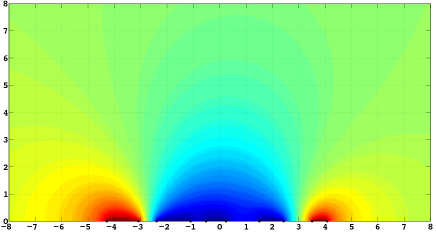
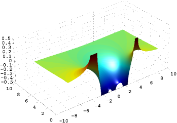
Figure 7: The graph of $\Re{\mathfrak{g}}(z)$, 2D (left) and 3D (right) views for an example of genus $g=4$.

Proposition 4.2.

(1) The function (4.4) satisfies the jump conditions

$${\mathfrak{g}}_{+}(z)+{\mathfrak{g}}_{-}(z)=-1~{}~{}~{}~{}{\rm on}~{}I_{i},~{}~{}~{}~{}~{}{\mathfrak{g}}_{+}(z)+{\mathfrak{g}}_{-}(z)=1~{}~{}~{}~{}{\rm on}~{}I_{e}$$ (4.5)

$$~{}{\rm and}~{}~{}~{}~{}~{}{\mathfrak{g}}_{+}(z)-{\mathfrak{g}}_{-}(z)=i\Omega_{j}~{}~{}~{}~{}{\rm on}~{}c_{j},~{}~{}j=0,1,\cdots,g-1,$$ (4.6)

where $\Omega_{0}=\frac{4}{i}\sum_{k=1}^{g}\int_{a_{2k-1}}^{a_{2k}}\!\!\!\!\!\omega_{1}dz\in{\mathbb{R}}$ and $\Omega_{j}=\frac{4}{i}\sum_{k=1}^{j}\int_{a_{2k-1}}^{a_{2k}}\!\!\!\!\!\omega_{1}dz\in{\mathbb{R}}$.
(2) The imaginary part of ${\mathfrak{g}}_{+}(z)$ satisfies

$$\Im{\mathfrak{g}}_{+}^{\prime}(z)=-2\Im\omega_{1}(z)\left\{\begin{array}[]{ll}>0&\ \ z\in I_{e},\\ <0&\ \ z\in I_{i}.\end{array}\right.$$ (4.7)

(3) Let $N_{i}$ denote a small neighborhood of $I_{i}$, so that $N_{i}\cap I_{e}=\varnothing$. Similarly, let $N_{e}$ denote a small neighborhood of $I_{e}$, so that $N_{e}\cap I_{i}=\varnothing$ ($N_{e}$ consists of two disjoint regions around $\gamma_{1}$ and $\gamma_{g+1}$, respectively). Then

$$\Re(2{\mathfrak{g}}(z)+1)>0,\ \ \ z\in N_{i}\setminus I_{i},\qquad\Re(2{\mathfrak{g}}(z)-1)<0,\ \ \ z\in N_{e}\setminus I_{e}.$$ (4.8)

(4) The function ${\mathfrak{g}}(z)$ is analytic in $\bar{\mathbb{C}}\setminus[a_{1},a_{2g+2}]$.

Proof.

(1) This follows from the fact that $R_{+}=-R_{-}$ on the corresponding sides of each main arc $\gamma_{j}$, $j=1,\dots,g+1$, and the normalization (4.2). In particular, if $z\in I_{e}$, then $\int_{a_{1}}^{z}\omega_{1}=0$, so the second jump condition (4.5) holds. If $z\in I_{i}$, then $\int_{a_{1}}^{z}\omega_{1}=1$ and the first jump condition (4.5) holds. Finally, (4.6) holds if $z\in c_{j}{=[a_{2j},a_{2j+1}]}$, $j=1,\dots,g-1$, or $z\in c_{0}{=[a_{2g},a_{2g+1}]}$, see Figure 6.

(2) Notice that $\arg R(z)=0$ when $z>a_{2g+2}$ and $\arg R_{+}(z)$ increases by $\frac{i\pi}{2}$ each time we pass a point $a_{j}$, $j=1,\cdots,2g+2$ from right to left. Then $\arg R_{+}(z)=\frac{i\pi}{2}$ when $z\in\gamma_{g+1}$ and $\arg R_{+}(z)=-\frac{i\pi}{2}$ when $z\in I_{i}$. According to Lemma 4.1, the polynomial $P_{1}(z)$, where $\omega_{1}=\frac{P_{1}(z)dz}{R(z)}$, has one zero in each $c_{j}$, $j=2,\cdots,g-1$. Thus the sign of $\Im\omega_{1}$ is the same on all the main arcs $\gamma_{k}\subset I_{i}$. The sign of $\Im\omega_{1}$ on the main arcs $\gamma_{1}$ and $\gamma_{g+1}$ (they form $I_{e}$) is also the same, but opposite to the sign on $I_{i}$. Since $\omega_{1}$ is positive on $c_{1}$, we conclude that $\Im\omega_{1}>0$ on $I_{i}$ and $\Im\omega_{1}<0$ on $I_{e}$. This implies (4.7).

(3) According to (1), $\Re(2{\mathfrak{g}}(z)+1)\equiv 0$ on $I_{i}$ and $\Re(2{\mathfrak{g}}(z)-1)\equiv 0$ on $I_{e}$. The imaginary part of ${\mathfrak{g}}_{+}$ is increasing on $I_{e}$. Hence, by Cauchy-Riemann equations, the real part is decreasing in the normal direction and thus the claim. A similar argument works for $I_{i}$.

(4) This follows from (4.4) and the integrability of $\omega_{1}$ as $z\rightarrow\infty$. ∎

We will also need an additional auxiliary function $d(z)$. To this end we first introduce the matrix

$$T=\mathbb{A}L=2\left[\begin{array}[]{c c c c}\int_{c_{1}}\frac{d\zeta}{R(\zeta)}&\cdots&\int_{c_{g-1}}\frac{d\zeta}{R(\zeta)}&\int_{c_{0}}\frac{d\zeta}{R(\zeta)}\\ \vdots&\vdots&\vdots&\vdots\\ \int_{c_{1}}\frac{\zeta^{g-1}d\zeta}{R(\zeta)}&\cdots&\int_{c_{g-1}}\frac{\zeta^{g-1}d\zeta}{R(\zeta)}&\int_{c_{0}}\frac{\zeta^{g-1}d\zeta}{R(\zeta)}\end{array}\right],$$ (4.12)

$$L=\left[\begin{array}[]{ccccc}1&0&\dots&0&-1\\ 0&1&0\dots&0&-1\\ &&\ddots&\\ &&\dots&1&-1\\ 0&0&\dots&0&1\end{array}\right]$$ (4.18)

and $\mathbb{A}$ is defined in (4.3). Then we define

$$d(z)=\frac{R(z)}{2\pi i}\left(-\sum_{j=1}^{g+1}\int_{\gamma_{j}}\frac{\ln w(\zeta)d\zeta}{(\zeta-z)R_{+}(\zeta)}+\sum_{j=0}^{g-1}\int_{c_{j}}\frac{{i\delta_{j}}d\zeta}{(\zeta-z)R(\zeta)}\right),$$ (4.19)

where the vector $\vec{\delta}=[\delta_{1},\dots,\delta_{g-1},\delta_{0}]^{t}$ is given by

$$\vec{\delta}=2\pi T^{-1}\left\{2\int_{a_{1}}^{\infty}-\int_{a_{1}}^{a_{2g+2}}\right\}\left[\begin{array}[]{c c }\frac{d\zeta}{R_{+}(\zeta)},\frac{\zeta d\zeta}{R_{+}(\zeta)},\dots,\frac{\zeta^{g-1}d\zeta}{R_{+}(\zeta)}\end{array}\right]^{t}.$$ (4.20)

Proposition 4.3.

The function $d(z)$given by (4.19) is analytic on $\bar{\mathbb{C}}\setminus[a_{1},a_{2g+2}]$ (in particular, analytic at infinity) and satisfies the jump conditions

$$d_{+}+d_{-}=-\ln w~{}~{}{\rm on~{}}\gamma_{j},~{}j=1,\dots g+1,~{}~{}~{}\qquad d_{+}-d_{-}=i\delta_{j}~{}~{}{\rm on~{}}c_{j},~{}j=0,\dots,g-1.$$ (4.21)

Proof.

Given the jump conditions (4.21), expression (4.19) follows from the Sokhotski–Plemelj formula. However, for an arbitrary $\vec{\delta}$, $d(z)=O(z^{g})$ as $z\rightarrow\infty$. Expanding $\frac{1}{\zeta-z}$ for large $z$ (and bounded $\zeta$), we obtain the system

$$\hskip 14.22636pti\sum_{j=0}^{g-1}\delta_{j}\int_{c_{j}}\frac{\zeta^{m}d\zeta}{R(\zeta)}=\sum_{j=1}^{g+1}\int_{\gamma_{j}}\frac{\zeta^{m}\ln w(\zeta)d\zeta}{R_{+}(\zeta)}=i\pi\left\{\int_{a_{2g+2}}^{\infty}+\int_{a_{1}}^{\infty}\right\}\frac{\zeta^{m}d\zeta}{R_{+}(\zeta)},$$ (4.22)

$${\rm where}~{}~{}m=0,1,\dots,g-1,$$

of $g$ linear equations for $g$ unknowns $\delta_{j}$, $j=0,1,\dots,g-1$, which is solved by (4.20). ∎

Using similar considerations, we calculate

$$\vec{\Omega}=-4iT^{-1}\sum_{l=2}^{g}\int_{\gamma_{l}}\left[\begin{array}[]{c c }\frac{d\zeta}{R_{+}(\zeta)},\frac{\zeta d\zeta}{R_{+}(\zeta)},\dots,\frac{\zeta^{g-1}d\zeta}{R_{+}(\zeta)}\end{array}\right]^{t},~{}~{}~{}~{}~{}$$ (4.23)

where $\vec{\Omega}=(\Omega_{1},\dots,\Omega_{g-1},\Omega_{0})^{t}$ and $\Omega_{j}$’s are the constants in (4.6).

Proposition 4.4.

The function ${\rm e}^{d(z)}$ has the behavior ${\rm e}^{d(z)}=C(z-a_{j})^{-\frac{1}{4}}(1+o(1))$ as $z\to a_{j}$, where $C\neq 0$, near the branchpoints $a_{j}$, $j=1,2g+2$, and is bounded at the remaining branchpoints $a_{j}$, $j=2,\cdots,2g+1$. As a consequence, the functions $\rho(z):=iw(z){\rm e}^{2d(z)}$ and $\frac{1}{\rho(z)}$ are bounded near $a_{1},a_{2g+2}$ (as well as near all the other branchpoints). Here $w(z)$ (cf. (1.4)) is understood as analytic on ${\mathbb{C}}\setminus(-\infty,a_{1}]\cup[a_{2g+2},\infty)$, and thus $\rho$ is analytic on ${\mathbb{C}}\setminus{\mathbb{R}}$.

Proof.

According to (4.19), $d(a_{j})=0$ for $j=2,\cdots,2g+1$. So, we consider the behavior of $d(z)$ at $z=a_{1}$, where $\ln w(\zeta)$ has a logarithmic singularity. According to [Gak66], Section 8.6, the behavior of $d(z)$ in a small neighborhood of $a_{1}$ and away from the cut $\gamma_{1}$ is given by

$$d(z)=-(z-a_{1})^{\frac{1}{2}}\frac{\ln(z-a_{1})-i\pi}{4(z-a_{1})^{\frac{1}{2}}}(1+o(1))=\left(-\frac{\ln(z-a_{1})}{4}+\frac{i\pi}{4}\right)(1+o(1)),$$ (4.24)

which implies the required behavior at $z=a_{1}$. Similar arguments work at $z=a_{2g+2}$. ∎

4.1 Transformation of the RHP

Let $\varkappa=-\ln\lambda$. Then $\varkappa>0$ when $\lambda\in(0,1)$ and $\varkappa\rightarrow\infty$ as $\lambda\rightarrow 0$. In this subsection we very briefly describe the nonlinear steepest descent method of Deift and Zhou, which allows to reduce the original RHP 3.10 to its leading order term, known as the model RHP (see RHP 4.7), in the limit $\varkappa\rightarrow+\infty$. The $g$–function ${\mathfrak{g}}(z)$ and, to a lesser extent, $d(z)$ are important parts of this reduction. A detailed description of the nonlinear steepest descent method can be found, for example, in [Dei99], [DZ92]. The first substitution

$$Y(z;\varkappa)=e^{-(\varkappa{\mathfrak{g}}_{\infty}+d_{\infty})\sigma_{3}}\Gamma(z;e^{-\varkappa})e^{(\varkappa{\mathfrak{g}}(z)+d(z))\sigma_{3}},$$ (4.25)

where $d(\infty)=d_{\infty}\in{\mathbb{C}}$ and ${\mathfrak{g}}(\infty)={\mathfrak{g}}_{\infty}\in{\mathbb{C}}$, reduces the RHP 3.10 to the following RHP.

Riemann-Hilbert Problem 4.5.

Find a $2\times 2$ matrix-function $Y(z;\varkappa)$ with the following properties:

1. $Y(z;\varkappa)$ is analytic in ${\mathbb{C}}\setminus[a_{1},a_{2g+2}]$;

2. $Y(z;\varkappa)$ satisfies the jump conditions

   $$\begin{split}Y_{+}&=Y_{-}\left[\begin{matrix}e^{(\varkappa{\mathfrak{g}}+d)_{+}-(\varkappa{\mathfrak{g}}+d)_{-}}&0\\ {iw}e^{\varkappa(\mathcal{{\mathfrak{g}}}_{+}+{\mathfrak{g}}_{-}+1)+d_{+}+d_{-}}&e^{-(\varkappa{\mathfrak{g}}+d)_{+}+(\varkappa{\mathfrak{g}}+d)_{-}}\end{matrix}\right],\ \ z\in I_{i},\\ Y_{+}&=Y_{-}\left[\begin{matrix}e^{(\varkappa{\mathfrak{g}}+d)_{+}-(\varkappa{\mathfrak{g}}+d)_{-}}&-\frac{i}{w}e^{-\varkappa(\mathcal{{\mathfrak{g}}}_{+}+{\mathfrak{g}}_{-}-1)-d_{+}-d_{-}}\\ 0&e^{-(\varkappa{\mathfrak{g}}+d)_{+}+(\varkappa{\mathfrak{g}}+d)_{-}}\end{matrix}\right],\ \ z\in I_{e}\\ &Y_{+}=Y_{-}e^{[(\varkappa{\mathfrak{g}}+d)_{+}-(\varkappa{\mathfrak{g}}+d)_{-}]\sigma_{3}},~{}~{}z\in[a_{2j},a_{2j+1}],~{}j=1,\dots,g;\end{split}$$ (4.26)

3. $Y={\bf 1}+O(z^{-1})~{}~{}~{}~{}{\rm as}~{}~{}z\rightarrow\infty,$ and;

4. Near the branchpoints (we indicate the behavior for the columns if these have different behaviors)

   $$\begin{split}Y(z;\varkappa)&=[\mathcal{O}(1),\mathcal{O}(z-a_{j})^{-\frac{1}{2}}],\ j=1,2g+2;\\ Y(z;\varkappa)&=O(\ln(z-a_{j})),~{}~{}~{}j=2,\dots,2g+1.\end{split}$$ (4.27)

The jump matrices in (4.26) can be calculated directly from (4.25) and (3.10). The branchpoint behavior (4.27) follows from Proposition 4.4 and (3.12)-(3.14), where we take into the account that the first column $\vec{A}(z)$ of $\Gamma(z;e^{-\varkappa})$ is analytic on $I_{e}$ (see the proof of Proposition 3.12).

We can now rewrite the jump conditions (4.26) as

$$\begin{split}Y_{+}&=Y_{-}\left[\begin{matrix}1&\frac{{\rm e}^{-\varkappa(2{\mathfrak{g}}_{{}_{-}}+1)-2d_{-}}}{iw}\\ 0&1\end{matrix}\right]\left[\begin{matrix}0&i\\ i&0\end{matrix}\right]\left[\begin{matrix}1&\frac{{\rm e}^{-\varkappa(2{\mathfrak{g}}_{{}_{+}}+1)-2d_{+}}}{iw}\\ 0&1\end{matrix}\right]\text{ on }I_{i},\\ Y_{+}&=Y_{-}\left[\begin{matrix}1&0\\ {iw}{{\rm e}^{\varkappa(2{\mathfrak{g}}_{{}_{-}}-1)+2d_{-}}}&1\end{matrix}\right]\left[\begin{matrix}0&-i\\ -i&0\end{matrix}\right]\left[\begin{matrix}1&0\\ {iw}{{\rm e}^{\varkappa(2{\mathfrak{g}}_{{}_{+}}-1)+2d_{+}}}&1\end{matrix}\right]\text{ on }I_{e},\\ Y_{+}&=Y_{-}{\rm e}^{i(\varkappa\Omega_{j}+\delta_{j}){\sigma}_{3}}\text{ on }c_{j},\ j=0,\dots g-1,\end{split}$$ (4.28)

which can be checked by direct matrix multiplication, together with the fact that $-\ln w-d_{+}-d_{-}\equiv 0$ on the main arcs and ${\mathfrak{g}}_{+}+{\mathfrak{g}}_{-}\pm 1\equiv 0$ on $I_{i}$ and $I_{e}$ respectively, see (4.5) and (4.21). In both factorizations of the jump matrices in (4.28) (on $I_{i}$ and $I_{e}$), the left and right (triangular) matrices admit analytic extension on the left/right vicinities of the corresponding main arcs because they are boundary values of analytic matrices in those vicinities. This suggests opening of the lenses $\partial\mathcal{L}_{e}^{(\pm)},~{}\partial\mathcal{L}_{i}^{(\pm)}$ around the corresponding main arcs, see Figure 8 top panel, and introduction of the new unknown matrix

$$Z(z;\varkappa)=\left\{\begin{array}[]{ll}Y(z;\varkappa)&\text{ outside the lenses,}\\ \displaystyle Y(z;\varkappa)\left[\begin{matrix}1&0\\ \mp{iw}{{\rm e}^{\varkappa(2{\mathfrak{g}}-1)+2d}}&1\end{matrix}\right]&z\in{\mathcal{L}_{e}^{(\pm)}},\\ \displaystyle Y(z;\varkappa)\left[\begin{matrix}1&\frac{\mp 1}{iw}{{\rm e}^{-\varkappa(2{\mathfrak{g}}+1)-2d}}\\ 0&1\end{matrix}\right]&z\in\mathcal{L}_{i}^{(\pm)}.\end{array}\right.$$ (4.32)

Figure 8: The regions of the lenses $\mathcal{L}^{(\pm)}_{i,e}$ (above) and the jumps of the error matrix $\mathcal{E}$ (below).

Consequently, the new matrix $Z$ satisfies the following RHP.

Riemann-Hilbert Problem 4.6.

Find the matrix $Z$, analytic on the complement of the arcs of Figure 8, top panel, satisfying the jump conditions (note also the orientations marked in Figure 8)

(4.33)

$$Z_{+}(z;\varkappa)=Z_{-}(z;\varkappa)\left\{\begin{array}[]{ll}{\rm e}^{i(\varkappa\Omega_{j}+\delta_{j}){\sigma}_{3}}&z\in c_{j},\ j=0,\dots g-1,\\ \left[\begin{matrix}1&0\\ {iw}{{\rm e}^{\varkappa(2{\mathfrak{g}}-1)+2d}}&1\end{matrix}\right]&z\in\partial\mathcal{L}_{e}^{(\pm)}\setminus{\mathbb{R}},\\ \left[\begin{matrix}1&\frac{1}{iw}{{\rm e}^{-\varkappa(2{\mathfrak{g}}+1)-2d}}\\ 0&1\end{matrix}\right]&z\in\partial\mathcal{L}_{i}^{(\pm)}\setminus{\mathbb{R}},\\ i{\sigma}_{1}&z\in I_{i},\\ -i{\sigma}_{1}&z\in I_{e},\end{array}\right.$$ (4.39)

normalized by

$$Z(z;\varkappa)\to{\bf 1}\ ,\ \ z\to\infty,$$ (4.40)

and with the same endpoint behavior as $Y$ near the endpoints $a_{j}$’s, see (4.27).

We shall provide a uniform approximation to the RHP 4.6 (which is entirely equivalent to the RHP 3.10 for $\Gamma$).

Since the real part of ${\mathfrak{g}}$ satisfies conditions (4.8), the off-diagonal entries in the jump matrices on the boundaries of the lenses of (4.33) tend exponentially to zero in any $L^{p}$ norm ($1\leq p<\infty$) on the lenses while away from the branchpoints $a_{j}$, $j=1,\cdots,2g+2$ as long as $\Re\varkappa\to+\infty$ and $\Im\varkappa$ remains bounded. Thus, neglecting the jumps on the lenses away from the branchpoints leads to exponentially small (in the limit $\varkappa\rightarrow+\infty$) errors. The error caused by the jumps on the parts of the lenses that are close to branchpoints require introduction of local parametrices. This will be considered in Subsection 4.2. If we completely neglect the jumps on the lenses, we arrive at the following “model problem” which captures the essence of the approximation.

Riemann-Hilbert Problem 4.7 (Model problem).

Find a matrix $\Psi=\Psi(z;\varkappa)$, analytic on ${\mathbb{C}}\setminus[a_{1},a_{2g+2}]$ and satisfying the following conditions:

$$\begin{split}&\Psi_{+}=\Psi_{-}(-1)^{s(j)}(i{\sigma}_{1})\ ,\ s(j)=\delta_{j,1}+\delta_{j,g+1},{\rm~{}on~{}}\gamma_{j},j=1,\dots g+1;\\ &\Psi_{+}=\Psi_{-}e^{i(\varkappa\Omega_{j}+\delta_{j})\sigma_{3}}{\rm~{}on~{}}c_{j},j=0,\dots,g-1;\\ &\Psi(z)=\mathcal{O}(|z-a_{j}|^{-\frac{1}{4}})\ ,\ \ z\to a_{j},\ j=1,\dots,2g+2;\\ &\Psi(z)={\bf 1}+\mathcal{O}(z^{-1})\ ,\ \ z\to\infty,~{}~{}{\rm and}~{}~{}\Psi_{\pm}(z)\in L^{2}([a_{1},a_{2g+2}]).\end{split}$$ (4.41)

Here $\delta_{j,k}$ denotes the Kronecker delta (not to be confused with the vector $\vec{\delta}$ and its components $\delta_{j}$ introduced in (4.19), (4.20)).

It is well known that solution to the RHP 4.7, if it exists, is unique. The proof of uniqueness proceeds analogously to the proof of Proposition 3.12. For our purposes, the most important information to extract from the Problem 4.7 is for what values of $\varkappa$ it is not solvable. This will be accomplished in section 5.

Proposition 4.8 (Symmetry).

If $\Psi(z;\varkappa)$ satisfies the RHP 4.7 then $\det\Psi\equiv 1$ and $\widetilde{\Psi}\equiv\Psi$, where $\widetilde{\Psi}(z;\varkappa)=\overline{\Psi(\bar{z};\overline{\varkappa})}$. In particular, for $\varkappa\in{\mathbb{R}}$, $\Psi_{j1+}(z;\varkappa)=\overline{\Psi}_{j1-}(z;\varkappa)$ for any $z\in I=I_{i}\cup I_{e}$.

The proof of these statements follows the same arguments used in the proof of Proposition 3.12 and Remarks 3.13, 3.14.

4.2 Local Riemann–Hilbert problems

The uniform approximation approach to $Z(z;\varkappa)$ requires that we analyze neighborhoods of the branchpoints (where the jump matrices on the lenses do not approach the identity in $L^{\infty}$ norm as $\Re(\varkappa)\to+\infty$.) We define the local coordinates $\xi_{j}(z)$ near each of the $a_{j}$’s to be

$$\sqrt{\xi_{j}}=\sqrt{\xi_{j}(z)}:=\varkappa\int_{a_{j}}^{z}\omega_{1}d\zeta=C_{j}\sqrt{z-a_{j}}(1+\mathcal{O}(z-a_{j}))\ ,$$ (4.42)

$$\ \ j=1,2,2g+1,2g+2,$$ (4.43)

$$\sqrt{\xi_{j}}=\sqrt{\xi_{j}(z)}:=-\varkappa\int_{a_{j}}^{z}\omega_{1}d\zeta=C_{j}\sqrt{z-a_{j}}(1+\mathcal{O}(z-a_{j}))\ ,$$ (4.44)

$$\ \ j=3,\dots,2g.$$

Inspecting the integrand, we see that the constants $C_{j}$ are given by $\pm\frac{2\varkappa P_{1}(a_{j})}{\sqrt{\prod_{k\neq j}(a_{k}-a_{j})}}$ and thus they do not vanish by Lemma 4.1. We choose the determination of $\xi_{j}$ always in such a way that the main arc originating at $z=a_{j}$ is mapped to the negative real axis by $\xi_{j}(z)$. Note that each $\xi_{j}$ is analytic in a full neighborhood of $a_{j}$ and each is a local conformal mapping. These local coordinates are clearly related to the function ${\mathfrak{g}}$ in view of (4.4), and, thus, also to the exponents appearing in the jump conditions of (4.28) near the $a_{j}$’s (from the $\pm$ sides of the real axis). Specifically, we have

$${\mathfrak{g}}(z)=\frac{1}{2}-2\int_{a_{j}}^{z}\omega_{1}d\zeta\ \Rightarrow\ \ \varkappa(2{\mathfrak{g}}(z)-1)=-4\sqrt{\xi_{j}},\ \ \ \ j=1,2g+2;$$

$${\mathfrak{g}}(z)=\frac{1}{2}\pm\frac{i}{{2}}\Omega_{1}-2\int_{a_{2}}^{z}\omega_{1}d\zeta\Rightarrow\ \ \varkappa(2{\mathfrak{g}}(z)-1)=\pm i\varkappa\Omega_{1}-4\sqrt{\xi_{2}},$$

$${\mathfrak{g}}(z)={-}\frac{1}{2}\pm\frac{i}{{2}}\Omega_{\lfloor\frac{\ell}{2}\rfloor}-2\int_{a_{\ell}}^{z}\omega_{1}d\zeta\Rightarrow\ \ -\varkappa(2{\mathfrak{g}}(z){+}1)=\mp i\varkappa\Omega_{\lfloor\frac{\ell}{2}\rfloor}-4\sqrt{\xi_{\ell}},\qquad\ \ \ell=3,4,\dots,2g,$$

$${\mathfrak{g}}(z)=\frac{1}{2}\pm\frac{i}{{2}}\Omega_{0}-2\int_{a_{2g+1}}^{z}\omega_{1}d\zeta\Rightarrow\ \ \varkappa(2{\mathfrak{g}}(z)-1)=\pm i\varkappa\Omega_{0}-4\sqrt{\xi_{2g+1}}.$$

In terms of these newly defined local coordinates $\xi_{j}$, the jump conditions in (4.33) become as indicated in Table 1. We shall need to construct local exact solutions of the jump conditions of the problem for $Z$ (see (4.33)) in the neighborhood of each branchpoint. The prototypical RHP near those branchpoints is summarized here:

Endpoint	Lenses	Main	Complementary	Orientation
$a_{1}$	$\displaystyle\left[\begin{matrix}1&0\\ {\rho}{\rm e}^{-4\sqrt{\xi_{1}}}&1\end{matrix}\right]$	$-i{\sigma}_{1}$	$\displaystyle{\bf 1}$	Out
$a_{2}$	$\displaystyle\left[\begin{matrix}1&0\\ {\rho}{\rm e}^{-4\sqrt{\xi_{2}}\pm i\varkappa\Omega_{1}}&1\end{matrix}\right]$	$\displaystyle-i{\sigma}_{1}$	$\displaystyle{\rm e}^{i(\varkappa\Omega_{1}+\delta_{1}){\sigma}_{3}}$	In
$a_{\ell}$	$\displaystyle\left[\begin{matrix}1&\frac{1}{\rho}{\rm e}^{-4\sqrt{\xi_{\ell}}\mp i\varkappa\Omega_{\lfloor\frac{\ell}{2}\rfloor}}\\ 0&1\end{matrix}\right]$	$\displaystyle i{\sigma}_{1}$	$\displaystyle{\rm e}^{i(\varkappa\Omega_{\lfloor\frac{\ell}{2}\rfloor}+\delta_{\lfloor\frac{\ell}{2}\rfloor}){\sigma}_{3}}$	odd $\ell$ Out; even $\ell$ In
$a_{2g+1}$	$\displaystyle\left[\begin{matrix}1&0\\ {\rho}\,{\rm e}^{-4\sqrt{\xi_{2g+1}}\pm i\varkappa\Omega_{0}}&1\end{matrix}\right]$	$\displaystyle-i{\sigma}_{1}$	$\displaystyle{\rm e}^{i(\varkappa\Omega_{0}+\delta_{0}){\sigma}_{3}}$	Out
$a_{2g+2}$	$\displaystyle\left[\begin{matrix}1&0\\ \rho{\rm e}^{-4\sqrt{\xi_{2g+2}}}&1\end{matrix}\right]$	$\displaystyle-i{\sigma}_{1}$	$\displaystyle{\bf 1}$	In

Table 1: The jump matrices of $Z$, see (4.33), near each of the endpoints are given in terms of the local coordinates $\xi_{j}$, $j=1,\dots,2g+2$. Here $\rho(z):=iw(z){\rm e}^{2d(z)}$. The little diagrams show the arcs near the endpoints $a_{j}$ and indicate the jump on the main arcs (lighter shade). The orientation “In/Out” refers to the lens and main arcs, and it means that they are oriented towards or away from $a_{j}$ (note that the complementary arc has the opposite orientation). The upper/lower choice of signs refers to the jumps on the lenses belonging to the upper or lower half-plane respectively.

Riemann-Hilbert Problem 4.9 (Local Bessel RHP).

Let $\vartheta\in(0,\pi)$ be any fixed number. Find a matrix $\mathcal{B}_{\nu}(\zeta)$ ($|\nu|<1$) that is analytic off the rays ${\mathbb{R}}_{-},{\rm e}^{\pm i\vartheta}{\mathbb{R}}_{+}$ and satisfies the following conditions (the contours oriented from the origin to infinity):

$$\mathcal{B}_{\nu+}(\zeta)=\mathcal{B}_{\nu-}(\zeta)\left[\begin{matrix}1&0\\ {\rm e}^{-4\sqrt{\zeta}\pm i\pi\nu}&1\end{matrix}\right],\ \ \zeta\in{\rm e}^{\pm i\vartheta}{\mathbb{R}}_{+};$$ (4.48)

$$\mathcal{B}_{\nu+}(\zeta)=\mathcal{B}_{\nu-}(\zeta)\left[\begin{matrix}0&1\\ -1&0\end{matrix}\right],\ \ \zeta\in{\mathbb{R}}_{-};$$ (4.49)

$$\mathcal{B}_{\nu}(\zeta)=\mathcal{O}(\zeta^{-\frac{|\nu|}{2}})\text{ for }\nu\neq 0\text{ or }\mathcal{O}(\ln\zeta)\text{ for }\nu=0\text{ as }\zeta\to 0;$$ (4.50)

$$\mathcal{B}_{\nu}(\zeta)=F(\zeta)\left({\bf 1}+\mathcal{O}(\zeta^{-\frac{1}{2}})\right),\ \ \zeta\to\infty,$$ (4.51)

$$F(\zeta):=(2\pi)^{-\sigma_{3}/2}\zeta^{-\frac{\sigma_{3}}{4}}\frac{1}{\sqrt{2}}\left[\begin{matrix}1&-i\\ -i&1\end{matrix}\right].$$

The solution to the RHP (4.9) was obtained in [Van07]. It is given (in a form convenient for our purposes) below.

$$\mathcal{B}_{\nu}(\zeta)=\begin{cases}\left[\begin{matrix}I_{\nu}(2\zeta^{\frac{1}{2}})&-\frac{i}{\pi}K_{\nu}(2\zeta^{\frac{1}{2}})\\[4.30554pt] -2\pi i\zeta^{\frac{1}{2}}I_{\nu}^{\prime}(2\zeta^{\frac{1}{2}})&-2\zeta^{\frac{1}{2}}K_{\nu}^{\prime}(2\zeta^{\frac{1}{2}})\end{matrix}\right]{\rm e}^{-2\sqrt{\zeta}{\sigma}_{3}},&\arg(\zeta)\in(-\vartheta,\vartheta),\\[21.52771pt] \left[\begin{matrix}\frac{1}{2}H_{\nu}^{(1)}(2(-\zeta)^{\frac{1}{2}})&-\frac{1}{2}H_{\nu}^{(2)}(2(-\zeta)^{\frac{1}{2}})\\[4.30554pt] -\pi\zeta^{\frac{1}{2}}(H_{\nu}^{(1)})^{\prime}(2(-\zeta)^{\frac{1}{2}})&\pi\zeta^{\frac{1}{2}}(H_{\nu}^{(2)})^{\prime}(2(-\zeta)^{\frac{1}{2}})\end{matrix}\right]{\rm e}^{-2\sqrt{\zeta}{\sigma}_{3}}e^{\frac{1}{2}\nu\pi i\sigma_{3}},&\arg(\zeta)\in(\vartheta,\pi),\\[21.52771pt] \left[\begin{matrix}\frac{1}{2}H_{\nu}^{(2)}(2(-\zeta)^{\frac{1}{2}})&\frac{1}{2}H_{\nu}^{(1)}(2(-\zeta)^{\frac{1}{2}})\\[4.30554pt] \pi\zeta^{\frac{1}{2}}(H_{\nu}^{(2)})^{\prime}(2(-\zeta)^{\frac{1}{2}})&\pi\zeta^{\frac{1}{2}}(H_{\nu}^{(1)})^{\prime}(2(-\zeta)^{\frac{1}{2}})\end{matrix}\right]{\rm e}^{-2\sqrt{\zeta}{\sigma}_{3}}e^{-\frac{1}{2}\nu\pi i\sigma_{3}},&\arg\zeta\in(-\pi,-\vartheta),\end{cases}$$ (4.52)

where $H_{\nu}^{(1)}$, $H_{\nu}^{(2)}$ denote Hankel’s functions (Bessel functions of the third kind) and $I_{\nu},K_{\nu}$ denote the modified Bessel functions (see, for example, [GR94]).

Remark 4.10.

The arbitrariness of $\vartheta$ is simply indicative of the fact that the rays can be freely moved within the indicated sector. For our purposes we can fix any $\vartheta\in(0,\pi)$ by requiring that the boundaries of the lenses are the preimages of straight lines in the respective $\xi_{j}(z)$ local coordinates, within the disks $\Delta_{j}$. For example $\theta=3\pi/4$ so as to match the shape indicated in Fig. 8.

Remark 4.11.

Although the shape of the contours supporting the jumps in the inner endpoints in Figure 1 resemble those of the Airy parametrix [DKM⁺99], the jump matrices are different. This is also an expected consequence of the fact that the behavior of the ${\mathfrak{g}}$-function near the branchpoints is like a square root rather than the power $\frac{3}{2}$.

Remark 4.12.

In our labeling, the constants $\Omega_{0},\delta_{0}$ are the jumps of ${\mathfrak{g}}(z)$ and $d(z)$, respectively, on the complementary arc $c_{0}=[a_{2g},a_{2g+1}]$. This can be seen from (4.6), (4.23) for ${\mathfrak{g}}$, and from (4.21), (4.20) – for $d(z)$.

4.3 Final approximation

We shall denote the final and uniform approximation to the matrix $Z(z;\varkappa)$ by $\widetilde{Z}(z;\varkappa)$.

The accuracy of this approximation to $Z$ (and, thus, ultimately to $\Gamma$) is discussed in Section 6 after the solvability of the model Problem 4.7 has been analyzed in Section 5.

Here and henceforth we denote by $\mathbb{D}_{j}$ the disks around the branchpoints $a_{j}$ of the same radius $r$, which should be sufficiently small so that the disks do not intersect each other, see Figure 8, lower panel. We also use the notation $\mathbb{D}_{j}^{\pm}=\mathbb{D}_{j}\cap\{\pm\Im z>0\}$. Then $\widetilde{Z}(z;\varkappa)$ is defined by

$$\widetilde{Z}(z;\varkappa):=\left\{\begin{array}[]{l l}\displaystyle\Psi(z)&\!\!\!\!\!\!\!\!\!\!\!\!z\in{\mathbb{C}}\setminus\bigcup_{j=1}^{2g+2}\mathbb{D}_{j},\\[7.74997pt] \displaystyle\Psi(z)\rho^{-\frac{{\sigma}_{3}}{2}}{\rm e}^{\pm\frac{i\pi}{4}{\sigma}_{3}}[F(\xi_{1})]^{-1}\mathcal{B}_{\frac{1}{2}}(\xi_{1})\rho^{\frac{{\sigma}_{3}}{2}}{\rm e}^{\mp\frac{i\pi}{4}{\sigma}_{3}}&z\in\mathbb{D}_{1}^{\pm},\\[7.74997pt] \displaystyle\Psi(z)\rho^{-\frac{{\sigma}_{3}}{2}}{\rm e}^{\mp\frac{i\varkappa}{2}\Omega_{1}{\sigma}_{3}}{{\sigma}_{3}}[F(\xi_{2})]^{-1}\mathcal{B}_{0}(\xi_{2}){{\sigma}_{3}}{\rm e}^{\pm\frac{i\varkappa}{2}\Omega_{1}{\sigma}_{3}}\rho^{\frac{{\sigma}_{3}}{2}}&\text{ in }\mathbb{D}_{2}^{\pm},\\ \\[7.74997pt] \displaystyle\Psi(z)\rho^{-\frac{{\sigma}_{3}}{2}}{\rm e}^{\mp\frac{i\varkappa}{2}\Omega_{k-1}{\sigma}_{3}}{{\sigma}_{1}}[F(\xi_{2k-1})]^{-1}\mathcal{B}_{0}(\xi_{2k-1}){{\sigma}_{1}}{\rm e}^{\pm\frac{i\varkappa}{2}\Omega_{k-1}{\sigma}_{3}}\rho^{\frac{{\sigma}_{3}}{2}}&z\in\mathbb{D}_{2k-1}^{\pm},\\ \\[7.74997pt] \displaystyle\Psi(z)\rho^{-\frac{{\sigma}_{3}}{2}}{\rm e}^{\mp\frac{i\varkappa}{2}\Omega_{k}{\sigma}_{3}}{{\sigma}_{3}}{{\sigma}_{1}}[F(\xi_{2k})]^{-1}\mathcal{B}_{0}(\xi_{2k}){{\sigma}_{1}}{{\sigma}_{3}}{\rm e}^{\pm\frac{i\varkappa}{2}\Omega_{k}{\sigma}_{3}}\rho^{\frac{{\sigma}_{3}}{2}}&z\in\mathbb{D}_{2k}^{\pm},\\ \\[7.74997pt] \displaystyle\Psi(z)\rho^{-\frac{{\sigma}_{3}}{2}}{\rm e}^{\mp\frac{i\varkappa}{2}\Omega_{0}{\sigma}_{3}}[F(\xi_{2g+1})]^{-1}\mathcal{B}_{0}(\xi_{2g+1}){\rm e}^{\frac{i\varkappa}{2}\Omega_{0}{\sigma}_{3}}\rho^{\frac{{\sigma}_{3}}{2}}&z\in\mathbb{D}_{2g+1}^{\pm},\\ \\[7.74997pt] \displaystyle\Psi(z){\rm e}^{\pm\frac{i\pi}{4}{\sigma}_{3}}\rho^{-\frac{{\sigma}_{3}}{2}}{{\sigma}_{3}}[F(\xi_{2g+2})]^{-1}\mathcal{B}_{\frac{1}{2}}(\xi_{2g+2}){{\sigma}_{3}}\rho^{\frac{{\sigma}_{3}}{2}}{\rm e}^{\mp\frac{i\pi}{4}{\sigma}_{3}}&z\in\mathbb{D}_{2g+2}^{\pm},\\ \end{array}\right.$$ (4.53)

where $F(\xi)$ was defined in (4.48).

Remark 4.13.

The function $\rho$, which is analytic in ${\mathbb{C}}\setminus{\mathbb{R}}$, was introduced in Proposition 4.4, and $w(z)=\sqrt{(z-a_{1})(a_{2g+2}-z)}$ is understood here as analytic on ${\mathbb{C}}\setminus(-\infty,a_{1}]\cup[a_{2g+2},\infty)$ and positive on $[a_{1},a_{2g+2}]$. Note that $\rho^{\frac{{\sigma}_{3}}{2}}={\rm e}^{\frac{i\pi}{4}{\sigma}_{3}}w^{\frac{{\sigma}_{3}}{2}}{\rm e}^{d{\sigma}_{3}}$ and $\rho_{+}^{\frac{{\sigma}_{3}}{2}}\rho_{-}^{\frac{{\sigma}_{3}}{2}}={\rm e}^{\frac{i\pi}{2}{\sigma}_{3}}$ on the main arcs, while $\rho_{+}^{\frac{{\sigma}_{3}}{2}}=\rho_{-}^{\frac{{\sigma}_{3}}{2}}{\rm e}^{i\delta_{j}{\sigma}_{3}}$ on the complementary arcs $c_{j}$. All of these properties follow from (4.21).

Remark 4.14.

In checking the properties at $a_{1},a_{2g+2}$ it should be reminded that the function $w(z)=\sqrt{(z-a_{1})(a_{2g+2}-z)}$ has the cuts extending on $(-\infty,a_{1}]\cup[a_{2g+2},\infty)$.

4.3.1 How the parametrices are constructed.

Here we explain the rationale behind formula (4.53). The expressions in each $\mathbb{D}_{j}$ of formula (4.53) are usually called (local) parametrices and thus we will conform to the accepted convention.

The main driving logic is that the proposed $\widetilde{Z}$ must fulfill:

• inside each disk $\mathbb{D}_{k}$ the jump conditions of $\widetilde{Z}(z;\varkappa)$ are exactly the same as those satisfied by $Z(z;\varkappa)$ (see Table 1) ;

• The jump conditions satisfied by $\widetilde{Z}$ across the boundary of each disk are of the form $\widetilde{Z}_{+}(z;\varkappa)=\widetilde{Z}_{-}(z;\varkappa)\left({\bf 1}+\mathcal{G}(z)\right)$, $z\in\partial\mathbb{D}_{j}$ where $\mathcal{G}(z):\partial\mathbb{D}_{j}\to SL_{2}({\mathbb{C}})$ is a matrix that tends to zero uniformly as $\varkappa\to\infty$ at a certain rate (which will turn out to be $\varkappa^{-1}$).

For the benefit of the reader we show how the jump conditions of $\widetilde{Z}$ match those of $Z$ in a “constructive” way, rather than simply checking them one by one post-facto.

Consider the case of the endpoint $a_{1}$. We start from the exact jumps of $Z$ as in Table 1 and by multiplication on the right by appropriate matrices from the second line of (4.53), we see how to reduce the jump matrices to the form that matches those of the Problem 4.9. (i) Multiply $Z\mapsto Z\,\rho^{-\frac{{\sigma}_{3}}{2}}$ so that on the lenses they become $\left[\begin{matrix}1&0\\ {\rm e}^{-4\sqrt{\xi_{1}}}&1\end{matrix}\right]$, and on the main arc it becomes $i{\sigma}_{2}$. However this introduces an additional jump on $(-\infty,a_{1}]\cap\mathbb{D}_{1}$ due to the jump of $w=\sqrt{(z-a_{1})(a_{2g+2}-z)}$ of the form ${\rm e}^{\frac{i\pi}{2}{\sigma}_{3}}$. To remove the latter (undesired) jump we (ii) multiply by ${\rm e}^{\pm\frac{i\pi}{4}{\sigma}_{3}}$ in the regions $\mathbb{D}_{1}^{\pm}$, respectively. This removes the additional jump on $\xi_{1}>0$ ($z<a_{1}$), but transforms the jump matrices on the lenses to $\left[\begin{matrix}1&0\\ {\rm e}^{-4\sqrt{\xi_{1}}\pm i\pi\frac{1}{2}}&1\end{matrix}\right]$, which now matches precisely those of Problem 4.9 with $\nu=\frac{1}{2}$. The jump matrix $i{\sigma}_{2}$ on the main arc does not undergo any change. Reversing the transformations, we can state that

$$\mathcal{B}_{\frac{1}{2}}(\xi_{1})\,\rho^{\frac{{\sigma}_{3}}{2}}{\rm e}^{\mp\frac{i\pi}{4}{\sigma}_{3}}$$ (4.54)

has exactly the same jump conditions as $Z(z,\varkappa)$ (and as $\widetilde{Z}(z,\varkappa)$) in the neighborhood $\mathbb{D}_{1}$. At the same time we may multiply (4.54) on the left by an arbitrary invertible matrix-function. We use this to our advantage in such a way that on the boundary $\partial\mathbb{D}_{1}$ this analytic prefactor matches the behavior of (4.54). To this end, consider $\Psi(z)\rho^{-\frac{{\sigma}_{3}}{2}}{\rm e}^{\pm\frac{i\pi}{4}{\sigma}_{3}}[F(\xi_{1})]^{-1}$: direct calculations show that it has no jumps near $a_{1}$ (note that $F(\xi_{1}){\rm e}^{\mp\frac{i\pi}{4}{\sigma}_{3}}\rho^{\frac{{\sigma}_{3}}{2}}$ is a local solution of the ”model” RHP near $a_{1}$). Thus, it has at worst a pole at $z=a_{1}$. However, simple power counting shows that it may have at most a square root singularity. Thus, it is analytic at $z=a_{1}$. We have established that

$$\widetilde{Z}(z;\varkappa)=\Psi(z)\rho^{-\frac{{\sigma}_{3}}{2}}{\rm e}^{\pm\frac{i\pi}{4}{\sigma}_{3}}\framebox{ $[F(\xi_{1})]^{-1}\mathcal{B}_{\frac{1}{2}}(\xi_{1})$}\rho^{\frac{{\sigma}_{3}}{2}}{\rm e}^{\mp\frac{i\pi}{4}{\sigma}_{3}}$$ (4.55)

in $\mathbb{D}_{1}$ has exactly the same jump conditions as $Z(z;\varkappa)$ inside $\mathbb{D}_{1}$. Now we examine this formula on the boundary of $\mathbb{D}_{1}$; here $\sqrt{\xi_{1}}=\varkappa\int_{a_{1}}^{z}\omega_{1}d\zeta$, so that $|\xi_{1}|=\mathcal{O}(\varkappa^{2})$. Thus the $[F(\xi_{1})]^{-1}\mathcal{B}_{\frac{1}{2}}(\xi_{1})$ term in (4.55) (the framed term), due to (4.48), behaves like

$$[F(\xi_{1})]^{-1}\mathcal{B}_{\frac{1}{2}}(\xi_{1})={\bf 1}+\mathcal{O}\left(\frac{1}{\varkappa}\right)\ ,$$ (4.56)

where the $\mathcal{O}$ term is uniform for $z\in\partial\mathbb{D}_{1}$. The details of the error analysis are deferred to section 6.

These steps have to be repeated for each of the branchpoints $a_{j}$. The overall result is summarized in the following proposition.

Proposition 4.15.

(1) The matrix $\widetilde{Z}(z;\varkappa)$ defined in (4.53) has exactly the same jumps as $Z(z;\varkappa)$ within $\mathbb{D}_{j}$ and on all main arcs $\gamma_{j}$.
(2) There is a constant $\mathcal{N}$, independent of $\varkappa$, such that

$$\widetilde{Z}_{+}(z;\varkappa)=\widetilde{Z}_{-}(z;\varkappa)({\bf 1}+\mathcal{O}(\varkappa^{-1}))\ ,\ \ \ z\in\partial\mathbb{D}_{j},~{}~{}~{}j=1,\cdots,2g+2.$$ (4.57)

with $|\mathcal{O}(\varkappa^{-1})|\leq\mathcal{N}/|\varkappa|$ for large $|\varkappa|$.
(3) The estimate above is valid uniformly as ${\Re\varkappa\to+\infty}$ and $\Im\varkappa$ remains bounded.

Proof.

Only the points (2),(3) have to be proven. The jump of $\widetilde{Z}$ is expressed in (4.55), since $\widetilde{Z}_{-}=\Psi$ and thus ($\nu_{1}=\nu_{2g+2}=\frac{1}{2},\nu_{j}=0$ otherwise)

$$\widetilde{Z}_{+}(z;\varkappa)(\widetilde{Z}_{-}(z;\varkappa))^{-1}=\rho^{-\frac{{\sigma}_{3}}{2}}{\rm e}^{\pm\frac{i\pi}{4}{\sigma}_{3}}[F(\xi_{j})]^{-1}\mathcal{B}_{\nu_{j}}(\xi_{j})\rho^{\frac{{\sigma}_{3}}{2}}{\rm e}^{\mp\frac{i\pi}{4}{\sigma}_{3}}.$$ (4.58)

In the right hand side the only dependence on $\varkappa$ is in $\xi_{j}$, and on the boundary of the disks $\mathbb{D}_{j}$ we have $|\xi_{j}(z)|>C|\varkappa|^{2}$. We then use property (4.48) of the Bessel parametrix: $[F(\xi_{j})]^{-1}\mathcal{B}_{\nu_{j}}(\xi_{j})={\bf 1}+\mathcal{O}(\xi_{j}^{-{\frac{1}{2}}})$. So, on the boundary of each disk $\mathbb{D}_{j}$, we have $[F(\xi_{j})]^{-1}\mathcal{B}_{\nu_{j}}(\xi_{j})={\bf 1}+\mathcal{O}(\varkappa^{-1})$. The last point (3) follows from the fact that the only dependence of (4.58) on $\varkappa$ is the factor $\varkappa$ in the definition of $\xi_{j}$ (cf. (4.42)). ∎

5 (Non)solvability of the model problem

The solution of the model RHP 4.7 was discussed in the literature, see, for example, [DKM⁺99, DIZ97, Kor04], where problems of this nature are solved in greater generality. Nonetheless, in this section we try to give a relatively brief but to a large degree self-contained exposition of solution of the RHP 4.7, using only some standard facts from the geometry of compact Riemann surfaces ([FK92, Fay73]). Some of this information can be found in Appendix A. We would like to remind the reader that our interest is not just in solving the RHP, but rather in knowing when it is not solvable. Reference [Kor04] turns out to be especially useful in this respect.

We recall the definition of the cycles $A,B$ (refer to Figure 6) and of the normalized first-kind differentials $\omega_{j}$ (4.3). The normalized matrix of $B$-periods is then

$$\tau=[\tau_{ij}]=\left[\oint_{B_{i}}\!\!\!\omega_{j}d\zeta\right]_{i,j=1,g}.$$ (5.1)

Theorem 5.1 (Riemann [FK92]).

The matrix $\tau$ is symmetric and its imaginary part is strictly positive definite.

In our case it is promptly seen from the definitions (4.3), (5.1) that $\tau$ is purely imaginary. The Abel map (of the first sheet of the Riemann surface) is defined to be

$$\mathfrak{u}(z)=\int_{a_{1}}^{z}\vec{\omega}(\zeta)d\zeta,\ \ \ \ z\in{\mathbb{C}}\setminus[a_{1},\infty).$$ (5.2)

Remark 5.2 (Abel map on the Riemann surface).

Here we have opted for the definition (5.2) which coincides with the one in the literature only on the first sheet. On occasions we will need the Abel map extended to a dense simply connected domain of the whole Riemann surface (the canonical dissection). When thinking of a point on the two sheets of the canonical dissection (i.e. a pair of values $p=(z,R(z))$) we shall use the symbol $\mathfrak{u}(p)$. The effect of the exchange of sheets is the change of sign of $\mathfrak{u}$. Also by the symbol $\mathfrak{u}(\infty)$ (without any subscript) we always denote the Abel map of the point at infinity on the first sheet, and if necessity arises we will use $\mathfrak{u}(\infty_{1,2})$ to distinguish between the two points at infinity on different sheets.

The aim of this section is to prove the following theorem:

Theorem 5.3.

The model RHP 4.7 is not solvable if and only if

$$\Theta\left(W-W_{0}\right)=0,$$ (5.3)

where $\Theta$ is the Riemann Theta-function, see Appendix A, and the vectors $W,W_{0}$ are given by

$$W=W(\varkappa)=\frac{\varkappa}{i\pi}\tau_{1}+2\mathfrak{u}(\infty)+\frac{{\bf e}_{1}}{2},\ \ W_{0}=\frac{\tau_{1}}{2}-\frac{{\bf e}_{1}+{\bf e}_{g}}{2}$$ (5.4)

with $\tau_{1}$ denoting the first column of the matrix $\tau$, and ${\bf e}_{j}$, $j=1,\dots,g$, being the vectors of the standard basis in ${\mathbb{C}}^{g}$.

Although this theorem can be derived from the results of [Kor04], we decided to give an independent proof below for the benefit of the reader and also because some notation will be needed in the sequel.

5.1 Proof of Theorem 5.3

The solution shall be written explicitly in terms of Theta-functions. Then, by inspection, we shall see that under special choices of $W$ there is a row-vector solution that tends to zero at infinity.

It is useful to keep in mind that our definition (5.2) of $\mathfrak{u}(z)$ leads to the following proposition, which was obtained by direct calculations.

Proposition 5.4 (Properties of the Abel map $\mathfrak{u}$).

The vector-valued function $\mathfrak{u}:{\mathbb{C}}\setminus[a_{1},\infty)$ defined in (5.2) satisfies

$$\mathfrak{u}(z)_{+}=-\mathfrak{u}(z)_{-}+\left\{\begin{array}[]{cl}0&z\in[a_{1},a_{2}],\\ \sum_{\ell=1}^{k}{\bf e}_{\ell}&z\in[a_{2k+1},a_{2k{+2}}]\ ,{1\leq}k\leq g-1,\\ {\bf e}_{g}&z\in[a_{2g+1},a_{2g+2}],\end{array}\right.$$ (5.8)

$$\mathfrak{u}(z)_{+}=\mathfrak{u}(z)_{-}+\left\{\begin{array}[]{cl}-\tau_{k}-\tau_{g}&z\in[a_{2k},a_{2k+1}]\ ,\ \ {1\leq}k\leq g-1,\\ -\tau_{g}&z\in[a_{2g},a_{2g+1}],\\ 0&z\in(-\infty,a_{1}]\cup[a_{2g+2},\infty),\end{array}\right.$$ (5.12)

where $\tau_{j}$ denotes the $j$-th column of the matrix $\tau$ in (5.1). In particular we have (all integrals taken on the $+$ side):

$$\begin{array}[]{ccc}\displaystyle\mathfrak{u}(a_{1})=0,&\displaystyle\mathfrak{u}(a_{2k+1})=\sum_{\ell=1}^{k}\frac{{\bf e}_{\ell}}{2}-\frac{\tau_{k}+\tau_{g}}{2},&\displaystyle\mathfrak{u}(a_{2g+1})=\frac{{\bf e}_{g}-\tau_{g}}{2},\\ \displaystyle\mathfrak{u}(a_{2k})=\sum_{\ell=1}^{k-1}\frac{{\bf e}_{\ell}}{2}-\frac{\tau_{k}+\tau_{g}}{2},&\displaystyle\mathfrak{u}(a_{2g})=\sum_{\ell=1}^{g-1}\frac{{\bf e}_{\ell}}{2}-\frac{\tau_{g}}{2},&\displaystyle\mathfrak{u}(a_{2g+2})=\frac{{\bf e}_{g}}{2}.\end{array}$$ (5.15)

Recall that $\mathcal{R}$ is hyperelliptic and, according to Proposition A.2 (see [FK92], p. 325, formula (1.2.1)), the vector $\mathcal{K}$ of Riemann constants is given by $\mathcal{K}=\sum_{j=1}^{g}\mathfrak{u}(a_{2j+1})$ (modulo periods). Thus, according to (5.15),

$$2\mathcal{K}=-g\tau_{g}-\sum_{k=1}^{g-1}\tau_{k}+{\bf e}_{g}+\sum_{\ell=1}^{g-1}(g-\ell){\bf e}_{\ell}.$$ (5.16)

Let us denote by $\Lambda_{\tau}={\mathbb{Z}}^{g}+\tau{\mathbb{Z}}^{g}\subset{\mathbb{C}}^{g}$ the lattice of periods. The Jacobian is the quotient $\mathbb{J}_{\tau}={\mathbb{C}}^{g}\mod\Lambda_{\tau}$ and it is a compact torus of real dimension $2g$ on account of Theorem 5.1.

Let now $J=\{1,5,7,9,11,\dots,2g-1\}$ and $J^{\prime}=\{1,2,3,\dots 2g+2\}\setminus J$ so that $|J|=g-1$ and $|J|^{\prime}=g+3$. The image of the degree $g-1$ divisor $\mathcal{D}_{J}=a_{1}+a_{5}+a_{7}+\dots+a_{2g-1}$ in the quotient $\mathbb{J}_{\tau}$ is

$$\mathfrak{u}(\mathcal{D}_{J}):=\sum_{j\in J}\mathfrak{u}(a_{j})=\mathcal{K}-\mathfrak{u}(a_{3})-\mathfrak{u}(a_{2g+1})=\mathcal{K}+\frac{\tau_{1}}{2}-\frac{{\bf e}_{1}+{\bf e}_{g}}{2}.$$ (5.17)

Lemma 5.5.

Define the functions

$$F_{1}^{(\pm)}(z):=\Theta\left(\mathfrak{u}(z)\mp\mathfrak{u}(\infty)-W_{0}\right),\qquad F_{2}^{(\pm)}(z):=\Theta\left(-\mathfrak{u}(z)\mp\mathfrak{u}(\infty)-W_{0}\right)$$ (5.18)

on ${\mathbb{C}}\setminus[a_{1},a_{2g+2}]$, where $W_{0}$ is given in (5.4). Then

• the vector $W_{0}$ in $\mathbb{J}_{\tau}$ equals

  $$W_{0}=\sum_{j\in J}\mathfrak{u}(a_{j})+\mathcal{K}.$$ (5.19)

• The functions $F_{1}^{{(+)}}(z),F_{2}^{{(-)}}(z)$ vanish at $z=\infty$;

• The functions $F_{1}^{{(-)}}(z),F_{2}^{{(+)}}(z)$ do not vanish at $z=\infty$;

• For each $j\in J$ they both vanish at $z=a_{j}$ like $\sqrt{z-a_{j}}$.

Proof.

Formula (5.19) follows by noticing that $\mathfrak{u}(a_{3})+\mathfrak{u}(a_{2g+1})=W_{0}$ (in $\mathbb{J}_{\tau}$) and using (5.17). We consider only the case $F_{k}^{(+)}$, $k=1,2$ (the case of $F_{k}^{(-)}$ is completely similar). In the following discussion we omit the super-index ⁽⁺⁾ for brevity. First, note that $F_{2}$ is the analytic continuation of $F_{1}$ across the cuts because of the jumps (5.8) and the periodicity properties of the Theta functions (A.3). Next we use the general Theorem A.3 which asserts that there are exactly $g$ zeroes of this extension on the whole Riemann surface $\mathcal{R}$. According to the definition of $W_{0}$, we have

$$\mathfrak{u}(\infty)+W_{0}=\mathfrak{u}(\infty)+\sum_{j\in J}\mathfrak{u}(a_{j})+\mathcal{K}.$$ (5.20)

Note that the divisor consisting of the points $\infty_{1,2},a_{j},j\in J$ ($\infty_{1,2}$ refer to the point at infinity on one or the other sheet, respectively) used in (5.20) on the hyperelliptic Riemann surface is non-special as recalled immediately after Definition A.7, and hence the $\Theta$ functions in the expressions for $F$ are not identically zero. Then, by Theorem A.5, the $g$ points $a_{j},~{}j\in J$ and $\infty_{1}$ (the infinity on the main sheet of $\mathcal{R}$) are the only zeroes of the extension of $F_{1}$. Whence the proof of the second and the fourth points. The third point is also proved because all the zeroes that the extension of $F_{1}$ on the second sheet can possibly have, have already been accounted for. Finally, the reason why the vanishing at $z=a_{j},\ j\in J$, is square-root like is due to the fact that the local coordinate in the Riemann surface near the branch point is $\sqrt{z-a_{j}}$. ∎

The functions $F_{1,2}^{(\pm)}(z)$ satisfy the jump conditions

$$F_{1}^{(\pm)}(z)_{+}=F_{2}^{(\pm)}(z)_{-},\quad z\in[a_{2k-1},a_{2k}],\ k=1,\dots g+1;$$ (5.21)

$$F_{1}^{(\pm)}(z)_{+}={\rm e}^{2i\pi V_{1}^{(\pm)}\cdot({\bf e}_{k}+{\bf e}_{g})-i\pi({\bf e}_{k}+{\bf e}_{g})\cdot\tau\cdot({\bf e}_{k}+{\bf e}_{g})}F_{1}^{(\pm)}(z)_{-},\quad z\in[a_{2k},a_{2k+1}]\ ,\ \ k=1,\dots g-1;$$ (5.22)

$$F_{1}^{(\pm)}(z)_{+}={\rm e}^{2i\pi V_{1}^{(\pm)}\cdot{\bf e}_{g}-i\pi{\bf e}_{g}\tau{\bf e}_{g}}F_{1}^{(\pm)}(z)_{-},\quad z\in[a_{2g},a_{2g+1}];$$ (5.23)

$$F_{2}^{(\pm)}(z)_{+}=F_{2}^{(\pm)}(z)_{-},\quad z\in\bigcup[a_{2k-1},a_{2k}];$$ (5.24)

$$F_{2}^{(\pm)}(z)_{+}={\rm e}^{-2i\pi V_{2}^{(\pm)}\cdot({\bf e}_{k}+{\bf e}_{g})-i\pi({\bf e}_{k}+{\bf e}_{g})\cdot\tau\cdot({\bf e}_{k}+{\bf e}_{g})}F_{2}^{(\pm)}(z)_{-},\quad z\in[a_{2k},a_{2k+1}]\ ,\ \ k=1,\dots g-1,$$ (5.25)

$$F_{2}^{(\pm)}(z)_{+}={\rm e}^{-2i\pi V_{2}^{(\pm)}\cdot{\bf e}_{g}-i\pi{\bf e}_{g}\tau{\bf e}_{g}}F_{2}^{(\pm)}(z)_{-},\quad z\in[a_{2g},a_{2g+1}],$$

where

$$V_{1}^{(\pm)}(z):=\mathfrak{u}(z)\mp\mathfrak{u}(\infty)-W_{0}\ ,\ \ \ V_{2}^{(\pm)}(z):=-\mathfrak{u}(z)\mp\mathfrak{u}(\infty)-W_{0}.$$ (5.26)

The jumps (5.21) follow from Propositions 5.4 and A.1.

Consider the function

$$h(z):=\sqrt[4]{\frac{\prod_{j\in J}(z-a_{j})}{\prod_{\ell\in J^{\prime}}(z-a_{\ell})}},\ \ \ z\in{\mathbb{C}}\setminus[a_{1},a_{2g+2}],$$ (5.27)

defined so that it is analytic in ${\mathbb{C}}\setminus[a_{1},a_{2g+2}]$ and at infinity behaves like $\frac{1}{z}$. Note that the points of the divisor $\mathcal{D}_{J}$ have been chosen to coincide with the finite zeroes of $h(z)$. Direct calculations show that:

$$h_{+}=ih_{-}\ ,\ z\in I_{i}=\bigcup_{k=1}^{g-1}[a_{2k+1},a_{2k+2}],$$ (5.28)

$$h_{+}=-h_{-}\ ,\ z\in[a_{2k},a_{2k+1}]\ ,k=2\dots,g,$$ (5.29)

$$h_{+}=-ih_{-}\ ,\ \ z\in I_{e}=[a_{1},a_{2}]\cup[a_{2g+1},a_{2g+2}],\$$ (5.30)

$$h_{+}=h_{-}\ ,\ \ \ z\in(\infty,a_{1}]\cup[a_{2},a_{3}]\cup[a_{2g+2},\infty).$$ (5.31)

The main solution of the problem is provided by the following theorem.

Theorem 5.6.

The matrix

$$\mathcal{M}(z):=\left[\begin{array}[]{cc}\displaystyle\frac{\Theta(\mathfrak{u}(z)-\mathfrak{u}(\infty)-W_{0}+W)h(z)}{\Theta(\mathfrak{u}(z)-\mathfrak{u}(\infty)-W_{0})}&\displaystyle\frac{\Theta(-\mathfrak{u}(z)-\mathfrak{u}(\infty)-W_{0}+W)h(z)}{\Theta(-\mathfrak{u}(z)-\mathfrak{u}(\infty)-W_{0})}\\[15.0pt] \displaystyle\frac{\Theta(\mathfrak{u}(z)+\mathfrak{u}(\infty)-W_{0}+W)h(z)}{\Theta(\mathfrak{u}(z)+\mathfrak{u}(\infty)-W_{0})}&\displaystyle\frac{\Theta(-\mathfrak{u}(z)+\mathfrak{u}(\infty)-W_{0}+W)h(z)}{\Theta(-\mathfrak{u}(z)+\mathfrak{u}(\infty)-W_{0})}\end{array}\right],$$ (5.34)

where $W\in{\mathbb{C}}^{g}$ is an arbitrary vector and $z\in{\mathbb{C}}\setminus[a_{1},a_{2g+2}]$, has the following properties:

• $\mathcal{M}(z)$ satisfies the jump conditions

  $$\mathcal{M}(z)_{+}=\mathcal{M}(z)_{-}\left[\begin{array}[]{cc}0&i\\ i&0\end{array}\right]\ ,\ \ z\in I_{i};\ \ \mathcal{M}(z)_{+}=\mathcal{M}(z)_{-}\left[\begin{array}[]{cc}0&-i\\ -i&0\end{array}\right]\ ,\ \ z\in I_{e};$$ (5.39)

  $$\mathcal{M}(z)_{+}=\mathcal{M}(z)_{-}\exp\left[\left(2i\pi W\cdot({\bf e}_{\ell}+{\bf e}_{g})+i\pi\sum_{k=2}^{g-1}\delta_{\ell k}\right)\sigma_{3}\right],$$ (5.40)

  $$\qquad\qquad\ \ z\in[a_{2\ell},a_{2\ell+1}]\ ,\ \ \ell\leq g-1;$$ (5.41)

  $$\mathcal{M}(z)_{+}=\mathcal{M}(z)_{-}\exp\left[\left(2i\pi W\cdot{\bf e}_{g}+i\pi\right)\sigma_{3}\right];$$ (5.42)

  $$\qquad\qquad\ \ \ z\in[a_{2g},a_{2g+1}];$$

• near any branchpoint $z=a_{j}$ each entry of $\mathcal{M}(z)$ is bounded by $|z-a_{j}|^{-\frac{1}{4}}$;

• $\mathcal{M}(z)$ has the behavior

  $$\mathcal{M}(z)=\Theta\left(W-W_{0}\right){C_{0}^{-1}}{\sigma}_{3}+\mathcal{O}(z^{-1})~{}~{}~{}~{}{\rm as}~{}~{}~{}z\rightarrow\infty,$$ (5.43)

  where $C_{0}\neq 0$ and

  $$C_{0}=[\mathbb{A}^{-1}\nabla\Theta(W_{0})]_{g}$$ (5.44)

  with $[N]_{g}$ denoting the $g$-th component of the vector $N$.

Proof.

(1) The proof of ((1)) follows from straightforward application of the periodicity properties of $\Theta$, see Proposition A.1 and the jump conditions (5.8) and (5.31).
(2) The function $h(z)$ from (5.27) behaves like $(z-a_{k})^{-\frac{1}{4}}$ at all branchpoints that are not in $J$. On the other hand, in each entry the denominators vanish at $z=a_{j}$, $j\in J$, like $\sqrt{z-a_{j}}$ by Lemma 5.5, while the function $h(z)$ vanishes like $(z-a_{j})^{\frac{1}{4}}$, $j\in J$. Thus each entry has the behavior $(z-a_{j})^{-\frac{1}{4}}$ at all the branchpoints.
(3) The boundedness follows because the denominators of the $(1,1)$ and $(2,2)$ entries vanish like $\frac{1}{z}$, but so does $h(z)$ at infinity. The off-diagonal entries $(1,2),(2,1)$ instead tend to zero because the denominators do not vanish (Lemma 5.5), while $h(z)$ still does. This proves that the leading order term of $\mathcal{M}$ at infinity is a diagonal matrix. To find this matrix, we calculate

$$\lim_{z\to\infty}\frac{\displaystyle\Theta\left(\int_{\infty}^{z}\vec{\omega}\,d\zeta-W_{0}\right)}{h(z)}=\lim_{z\to\infty}z\Theta\left(\int_{\infty}^{z}\!\!\!\vec{\omega}\,d\zeta-W_{0}\right).$$ (5.45)

The computation of this last limit is done using l’Hopital’s rule and taking into account (4.3) and the parity of $\Theta$:

$$\begin{split}\lim_{z\to\infty}-z^{2}\frac{d}{dz}\Theta\left(\int_{\infty}^{z}\!\!\!\!\vec{\omega}\,d\zeta-W_{0}\right)&=\lim_{z\to\infty}-z^{2}\vec{\omega}^{t}(z)\nabla\Theta\left(\int_{\infty}^{z}\!\!\!\!\vec{\omega}\,d\zeta-W_{0}\right)\\ &=-[\mathbb{A}^{-1}\nabla\Theta(-W_{0})]_{g}=[\mathbb{A}^{-1}\nabla\Theta(W_{0})]_{g}.\end{split}$$ (5.46)

Repeating the computation (5.46) for the entry $(2,2)$ of (5.43) gives $-[\mathbb{A}^{-1}\nabla\Theta(W_{0})]_{g}$. The fact that $C_{0}\neq 0$ is a consequence of Theorem A.3. Indeed $\Theta\left(\mathfrak{u}(z)-W_{0}\right)$ has a simple zero at $z=\infty$ (i.e. vanishes linearly in $1/z$) because the other $g-1$ zeroes are at $z=a_{j},~{}j\in J$, as stated in Lemma 5.5. ∎

We can restate Theorem 5.6 as follows.

Theorem 5.7.

Let

$$\Psi(z;W):=C_{0}\left[\begin{array}[]{cc}\displaystyle\frac{\Theta(\mathfrak{u}(z)-\mathfrak{u}(\infty)-W_{0}+W)h(z)}{\Theta(W-W_{0})\Theta(\mathfrak{u}(z)-\mathfrak{u}(\infty)-W_{0})}&\displaystyle\frac{\Theta(-\mathfrak{u}(z)-\mathfrak{u}(\infty)-W_{0}+W)h(z)}{\Theta(W-W_{0})\Theta(-\mathfrak{u}(z)-\mathfrak{u}(\infty)-W_{0})}\cr\displaystyle\frac{-\Theta(\mathfrak{u}(z)+\mathfrak{u}(\infty)-W_{0}+W)h(z)}{\Theta(W-W_{0})\Theta(\mathfrak{u}(z)+\mathfrak{u}(\infty)-W_{0})}&\displaystyle\frac{-\Theta(-\mathfrak{u}(z)+\mathfrak{u}(\infty)-W_{0}+W)h(z)}{\Theta(W-W_{0})\Theta(-\mathfrak{u}(z)+\mathfrak{u}(\infty)-W_{0})}\end{array}\right],$$ (5.49)

be a matrix function in ${\mathbb{C}}\setminus[a_{1},a_{2g+2}]$, where $W_{0}$ is given by (5.4) and $W\in{\mathbb{C}}^{g}$ is an arbitrary vector such that $\Theta(W-W_{0})\neq 0$. Then:
(1) this matrix has the same jumps as in ((1)) and $\det\Psi\equiv 1$.
(2) $\Psi(z)=O((z-a_{j})^{-\frac{1}{4}})$ near each $a_{j}$, $j=1,\cdots,2g+2$;
(3) at infinity the matrix tends to ${\bf 1}$;
(4) The constant $C_{0}\neq 0$ and is independent of $W$;
(5) The matrix $\Psi(z;W)$ is invariant under integer shifts of the vector $W$, $W\mapsto W+{\mathbb{Z}}^{g}$ (i.e. it is periodic in each component of $W$ along the real direction.).

Only the last item needs additional verification, but this follows from the fact that all theta functions have said periodicity.

For the rest of the paper, we will use notation $\Psi(z;\varkappa)=\Psi(z;W(\varkappa))$, where $\Psi(z;W)$ is defined in Theorem 5.7.

Corollary 5.8.

The RHP with jumps as in ((1)), the branchpoint behavior $O((z-a_{j})^{-\frac{1}{4}})$, $j=1,\cdots,2g+2,$ and bounded behavior at infinity admits a nontrivial solution vanishing at infinity if and only if the vector $W\in{\mathbb{C}}^{g}$ is such that

$$\Theta\left(W-W_{0}\right)=0.$$ (5.50)

Proof.

The sufficiency is obvious from (5.43). Suppose now $\Theta\left(W-W_{0}\right)\neq 0$. Then, according to (5.43), $\lim_{z\rightarrow\infty}\Psi(z)={\bf 1}$. But the solution of this normalized RHP is unique by the same arguments that were used in the proof of Proposition 3.12. The existence of a solution that vanishes at infinity would violate this uniqueness. ∎

Proof of Theorem 5.3..

To complete the proof of the theorem, we must find the vector $W$ so that the jump matrices in ((1)) are the same as those of $\Psi$ in (4.41). Comparing them, we see that the vector $W$ must satisfy

$$2\pi L\cdot W+\pi\sum_{\ell=2}^{g}{\bf e}_{\ell}=\varkappa\vec{\Omega}+\vec{\delta},$$ (5.51)

where $L$, $\vec{\delta},\vec{\Omega}$ are given by (4.12), (4.20) and (4.23), respectively. Then, according to (4.12), (4.23) and (4.20),

$$\vec{\Omega}=-2iL^{-1}\tau_{1}\ ,\ \ \ \vec{\delta}=2\pi L^{-1}\left(2\mathfrak{u}(\infty)-\mathfrak{u}(a_{2g+2})\right).$$ (5.52)

Thus, in view of (5.15),

$$W=\frac{\varkappa}{i\pi}\tau_{1}+2\mathfrak{u}(\infty)-\mathfrak{u}(a_{2g+2})+\frac{1}{2}{\bf e}_{1}-\frac{1}{2}{\bf e}_{g}=\frac{\varkappa}{i\pi}\tau_{1}+2\mathfrak{u}(\infty)+\frac{{\bf e}_{1}}{2}-{\bf e}_{g}.$$ (5.53)

The proof of Theorem 5.3 now follows from Theorem 5.6 and Corollary 5.8. Note that since $\Theta$ is periodic in ${\mathbb{Z}}^{g}$, the last term ${\bf e}_{g}$ is irrelevant. ∎

Definition 5.9.

The values $\varkappa^{exact}_{n}=-\ln\lambda_{n}$, where $n\in N$ and $\lambda_{n}>0$, for which the RHP (3.10) for $\Gamma(z;\lambda_{n})$ does not have a solution, we will call (with a mild abuse of terminology) exact eigenvalues of the RHP (3.10) or simply exact eigenvalues. The values $\varkappa_{n}$, $n\in N$, for which the model RHP (4.7) does not have a solution, will be called approximate eigenvalues.

According to Theorem 3.17, $\lambda_{n}={\rm e}^{-\varkappa_{n}^{exact}}$ are positive eigenvalues of the compact integral operator $\widehat{K}$, so that $\varkappa=+\infty$ is the only possible point of accumulation of the exact eigenvalues $\varkappa^{exact}_{n}$. Since the RHP 4.7 “approximates” the RHP (3.10), one can expect that the approximate eigenvalues $\varkappa_{n}$ will approximate the exact eigenvalues $\varkappa^{exact}_{n}$ as $n\rightarrow\infty$. This question will be explored in Section 6 below.

Remark 5.10.

So far we have not mentioned any particular way of enumerating the approximate eigenvalues $\varkappa_{n}$. Because of the expected approximation of exact eigenvalues, we shall assume that this enumeration is chosen in such a way that $\varkappa_{n}$ is “close” to $\varkappa^{exact}_{n}$ for sufficiently large $n\in{\mathbb{N}}$.

6 Error estimates

In order to estimate the difference between the exact solution $Z(z;\varkappa)$ of the RHP 4.6 and its approximation $\widetilde{Z}(z;\varkappa)$, we introduce the error matrix

$$\mathcal{E}(z;\varkappa):=Z(z;\varkappa)\widetilde{Z}^{-1}(z;\varkappa)\ .$$ (6.1)

We note that the jumps of $\widetilde{Z}$ are the same as those of $Z(z;\varkappa)$, see (4.33), on the main arcs and, within each disk $\mathbb{D}_{j}$, on the complementary arcs. Thus the only jump discontinuities of $\mathcal{E}$ are on the boundaries $\partial\mathbb{D}_{j}$ and across the boundaries of the lenses (on the lenses for briefness) outside of these disks, see Figure 8, bottom panel. According to (4.33) and (4.53), the jump matrices on the lenses are of the form

$$\mathcal{E}^{-1}_{-}(z;\varkappa)\mathcal{E}_{+}(z;\varkappa)=\Psi(z;\varkappa)\left({\bf 1}+{\sigma}_{\pm}{\rm e}^{\mp\varkappa(2g\pm 1)}(\rho)^{\mp 1}\right)\Psi^{-1}(z;\varkappa),$$ (6.2)

where the two signs refer to the lenses $\partial\mathcal{L}^{(\pm)}_{i}$ and $\partial\mathcal{L}^{(\pm)}_{e}$ around the intervals $I_{i}$ and $I_{e}$, respectively (see (4.33)). We can always assume that $\partial\mathcal{L}^{(\pm)}_{i}\subset N_{i}$ and $\partial\mathcal{L}^{(\pm)}_{e}\subset N_{e}$, where the regions $N_{i},N_{e}$ were defined in Proposition 4.2, part (3). Thus, according to the sign conditions (4.8), the factor ${\rm e}^{\mp\varkappa(2g\pm 1)}$ in (6.2) is exponentially small as $\Re\varkappa\to+\infty$ and $\Im\varkappa$ is bounded (say in $[-\pi/2,\pi/2]$). This exponential decay is uniform on the lenses (outside the corresponding disks $\mathbb{D}_{j}$). Since the remaining factors in (6.2) are bounded on the lenses (outside the disks), we see that the jumps of $\mathcal{E}$ outside the disks tend to ${\bf 1}$ exponentially fast and uniformly in $z$ as $\Re\varkappa\rightarrow+\infty$. The jumps of $\mathcal{E}$ on the boundary of the disks $\partial\mathbb{D}_{\ell}$ , according to (4.57), are

$$\mathcal{E}_{+}(z;\varkappa) =\mathcal{E}_{-}(z;\varkappa)\widetilde{Z}_{-}(z;\varkappa)\widetilde{Z}^{-1}_{+}(z;\varkappa)$$ (6.5)

$$=\mathcal{E}_{-}(z;\varkappa)\Psi(z;\varkappa)\rho^{-\frac{{\sigma}_{3}}{2}}{\rm e}^{\pm\frac{i\pi}{4}{\sigma}_{3}}F^{-1}(\xi_{j})\mathcal{B}_{\nu_{j}}(\xi_{j})\rho^{\frac{{\sigma}_{3}}{2}}{\rm e}^{\mp\frac{i\pi}{4}{\sigma}_{3}}\Psi^{-1}(z;\varkappa)$$

$$=\mathcal{E}_{-}(z;\varkappa)\Psi\rho^{-\frac{{\sigma}_{3}}{2}}({\bf 1}+\mathcal{O}(\varkappa^{-1}))\rho^{\frac{{\sigma}_{3}}{2}}\Psi^{-1}.$$

Consider now the expression for $\Psi(z;W)$ in Theorem 5.7: the reader can verify that if $\|\Im W\|$ is bounded, then the supremum of each entry as $z$ ranges on the boundaries $\partial\mathbb{D}_{\ell}$ is bounded as follows:

$$\max_{\ell\leq 2g+2}\sup_{z\in\mathbb{D}_{\ell}}|\Psi_{ij}|\leq\frac{N}{|\Theta(W-W_{0})|}\ .$$ (6.6)

with $N>0$ some constant. Then the jumps on $\partial\mathbb{D}_{\ell}$ of $\mathcal{E}$ in (6.5) are uniformly close to the identity jump to within $\mathcal{O}(\varkappa^{-1})/|\Theta(W(\varkappa)-W_{0})|^{2}$, that is

$$\mathcal{E}_{+}(z;\varkappa)=\mathcal{E}_{-}(z;\varkappa)\left({\bf 1}+\frac{\mathcal{O}(\varkappa^{-1})}{|\Theta(W(\varkappa)-W_{0})|^{2}}\right),$$ (6.7)

where $W=W(\varkappa)$ is defined by (5.53). We have already established that if $\Re\varkappa$ is sufficiently large (and $\Im\varkappa$ is bounded by some constant) then the jumps on the lenses outside of the disks are $\mathcal{O}({\rm e}^{-c|\varkappa|})$ small, for some $c>0$.

Let us consider a matrix RHP for some $G(z)$ with a jump matrix $V(z)$ on a contour $\Sigma$ and normalized by ${\bf 1}$ at $z=\infty$. Moreover, let the limiting matrices $G_{\pm}(z)\in L^{2}(\Sigma)$. It is well known (under the general title of “small norm theorem”) that if the $L^{2}$ and $L^{\infty}$ norms of $V(z)-{\bf 1}$ are sufficiently small then the RHP is solvable in terms of a convergent Neumann series and the solution $G(z)$ is also “close” to ${\bf 1}$ , see for example Ch. 7 in [Dei99]. In the case of the error matrix $\mathcal{E}$,   $V(z)-{\bf 1}$ becomes small as $\Re\varkappa\to+\infty$ in any $L^{p}$ norm. The largest contribution to $V(z)-{\bf 1}$ comes from the boundaries of $\mathbb{D}_{\ell}$, and its estimate can be seen from (6.7). Thus, $\mathcal{E}(z;\varkappa)$ exists and is close to ${\bf 1}$ if $\varkappa$ is sufficiently large. In turn, the solvability of the RHP for $\mathcal{E}$ implies the solvability of the RHP 3.10 by reverting the chain of exact transformations

$$\Gamma\mathop{\longrightarrow}^{\eqref{y-def}}Y\mathop{\longrightarrow}^{\eqref{422}}Z\mathop{=}^{\eqref{approx}}\mathcal{E}\widetilde{Z}.$$ (6.8)

Since the solvability of RHP (3.10) implies the absence of (exact) eigenvalues, there are no exact eigenvalues as long as the error term in (6.7) is smaller than a suitable constant, namely, in the region

$$\Re\varkappa>R_{0};\ \ \left|\Theta(W(\varkappa)-W_{0})\right|>\frac{C}{\sqrt{|\varkappa|}}$$ (6.9)

for suitable constants $R_{0},C>0$.

Recall that the positive approximate eigenvalues $\varkappa_{n}$ are defined by the equation $\Theta(W(\varkappa)-W_{0})=0$. We shall show in Lemma 7.7 that $\Theta(W(\varkappa)-W_{0})$ has only simple zeroes $\varkappa=\varkappa_{n}$, and $\frac{d}{d\varkappa}\Theta(W(\varkappa)-W_{0})\big{|}_{\varkappa=\varkappa_{n}}$ is bounded away from zero uniformly in $n$. Thus it follows from (6.9) that the exact eigenvalues $\varkappa_{n}^{exact}$ can only be found in small $\mathcal{O}(\varkappa^{-\frac{1}{2}})$-size neighborhoods of the approximate eigenvalues. In the following Subsection 6.1 we shall see that (asymptotically) near each approximate eigenvalue $\varkappa_{n}$ there is precisely one exact eigenvalue of multiplicity one.

6.1 The location of the eigenvalues

The core of this section is the proof of the following theorem.

Theorem 6.1.

If $n\in{\mathbb{N}}$ is sufficiently large, then there is exactly one exact eigenvalue $\varkappa_{n}^{exact}$ within a distance

$$|\varkappa_{n}^{exact}-\varkappa_{n}|=\mathcal{O}({\varkappa_{n}}^{-\frac{1}{2}})$$ (6.10)

of each approximate eigenvalue $\varkappa_{n}$.

Proof.

The bound on the distance has already been argued after (6.9), but the actual existence of an exact eigenvalue within a neighborhood of $\varkappa_{n}$ has not yet been established. We shall show that on a small disk around each $\varkappa_{n}$ (for $n$ sufficiently large) there is exactly one exact eigenvalue $\varkappa_{n}^{exact}$. We start our analysis with Proposition 3.20. Since the integral in Proposition 3.20 is on the cycle $B_{1}$ (denoted by $\hat{I}_{i}$ in (3.37)) that avoids the branchpoints, we have

$$\Gamma(z;{\rm e}^{-\varkappa})={\rm e}^{(d_{\infty}+\varkappa{\mathfrak{g}}_{\infty}){\sigma}_{3}}\mathcal{E}(z;\varkappa)\Psi(z;\varkappa){\rm e}^{-(\varkappa{\mathfrak{g}}(z)+d(z)){\sigma}_{3}},$$ (6.11)

where $z\in B_{1}$. Note that $\lambda={\rm e}^{-\varkappa}$ and, thus, $-\lambda\partial_{\lambda}=\partial_{\varkappa}$. Inserting (6.11) into Proposition 3.20 and taking into account (4.4), we obtain

$$\partial_{\varkappa}\ln\det\left(\mathrm{Id}-\frac{1}{\lambda}K\right) =-\lambda\partial_{\lambda}\ln\det\left(\mathrm{Id}-\frac{1}{\lambda}K\right)=\oint_{B_{1}}\left(\Gamma_{21}\Gamma_{12}^{\prime}-\Gamma_{11}\Gamma_{22}^{\prime}\right)\frac{dz}{i\pi}$$ (6.14)

$$=\oint_{B_{1}}\left(\Psi_{21}\Psi_{12}^{\prime}-\Psi_{11}\Psi_{22}^{\prime}\right)\frac{dz}{i\pi}-\oint_{B_{1}}(\varkappa{\mathfrak{g}}^{\prime}(z)+d^{\prime}(z))\frac{dz}{i\pi}+\mathcal{O}(\varkappa^{-1})$$

$$=\oint_{B_{1}}\left(\Psi_{21}\Psi_{12}^{\prime}-\Psi_{11}\Psi_{22}^{\prime}\right)\frac{dz}{i\pi}+\frac{2\varkappa}{i\pi}\tau_{11}-\oint_{B_{1}}d^{\prime}(z)\frac{dz}{i\pi}+\mathcal{O}(\varkappa^{-1}).$$

Here we have used the fact that $\mathcal{E}(z;\varkappa)$ is analytic in $z$ in a neighborhood of $B_{1}$ and uniformly close to the identity matrix ${\bf 1}$, and thus, by Cauchy’s theorem, also its derivative $\mathcal{E}_{z}(z;\varkappa)$ is uniformly $\mathcal{O}(\varkappa^{-1})$ on $B_{1}$. This approximation is uniform as long as $\varkappa-\varkappa_{n}$ remains bounded away from $0$ even if $\varkappa$ is allowed to take complex values and $\Re\varkappa\to\infty$.

To compute the number of eigenvalues lying within the disk $|\varkappa-\varkappa_{n}|<\epsilon$, we evaluate the integral (in $d\varkappa$) of both sides of equation (6.14) along the circle $|\varkappa-\varkappa_{n}|=\epsilon$. The only term in (6.14) which may have a pole at $\varkappa=\varkappa_{n}$ is the first integral, which we now set out to compute.

We start with observing that

$$Q(z):=\Psi_{21}(z)\Psi_{12}^{\prime}(z)-\Psi_{11}(z)\Psi_{22}^{\prime}(z)=\lim_{x\to z}\frac{1}{x-z}\left(1-\det\left[\begin{matrix}\Psi_{11}(z)&\Psi_{12}(x)\\ \Psi_{21}(z)&\Psi_{22}(x)\end{matrix}\right]\right)$$ (6.15)

and thus we want to compute the determinant appearing above.

Lemma 6.2.

We have

$$S(x,z):=\frac{1}{x-z}\det\left[\begin{matrix}\Psi_{11}(z)&\Psi_{12}(x)\\ \Psi_{21}(z)&\Psi_{22}(x)\end{matrix}\right]=\frac{C_{0}h(z)h(x)\Theta(\mathfrak{u}(z)-\mathfrak{u}(x)+W-W_{0})}{\Theta(\mathfrak{u}(z)-\mathfrak{u}(x)-W_{0})\Theta(W-W_{0})},$$ (6.16)

where $C_{0}$ is defined by (5.44).

Proof.

Refer to the matrix $\Psi$ in Theorem 5.7. Factoring out $h(z)h(x)$, which appears on both sides, identity (6.16) amounts to

$$\det\left[\begin{array}[]{cc}\displaystyle\frac{C_{0}\Theta(\mathfrak{u}(z)-\mathfrak{u}(\infty)+W-W_{0})}{\Theta(W-W_{0})\Theta(\mathfrak{u}(z)-\mathfrak{u}(\infty)-W_{0})}&\displaystyle\frac{C_{0}\Theta(-\mathfrak{u}(x)-\mathfrak{u}(\infty)+W-W_{0})}{\Theta(W-W_{0})\Theta(-\mathfrak{u}(x)-\mathfrak{u}(\infty)-W_{0})}\cr\displaystyle\frac{-C_{0}\Theta(\mathfrak{u}(z)+\mathfrak{u}(\infty)+W-W_{0})}{\Theta(W-W_{0})\Theta(\mathfrak{u}(z)+\mathfrak{u}(\infty)-W_{0})}&\displaystyle\frac{-C_{0}\Theta(-\mathfrak{u}(x)+\mathfrak{u}(\infty)+W-W_{0})}{\Theta(W-W_{0})\Theta(-\mathfrak{u}(x)+\mathfrak{u}(\infty)-W_{0})}\end{array}\right]$$ (6.19)

$$=\frac{C_{0}(x-z)\Theta(\mathfrak{u}(z)-\mathfrak{u}(x)+W-W_{0})}{\Theta(\mathfrak{u}(z)-\mathfrak{u}(x)-W_{0})\Theta(W-W_{0})}.$$ (6.20)

This is an instance of the famous Fay identities ([Fay73], page 33). The idea is to compare the two sides of (6.20) as functions of $z,x$ and verify that they have the same poles and the same periodicity around the $A,B$ cycles. Then a simple argument using the non-specialty of the divisor of degree $g$ whose image is $W-W_{0}-\mathcal{K}$, proves that they must be proportional to each other. Evaluation of the proportionality constant is achieved by noticing that the left side of (6.20) tends to $[h(z)]^{-2}$ when $z=x$ (because it gives exactly $[h(z)]^{-2}\det\Psi(z)$, where $\det\Psi\equiv 1$, see Theorem 5.7). Observe now the right hand side: expression (A.8) from Lemma A.8 implies that $\lim_{x\to z}\frac{x-z}{\Theta(\mathfrak{u}(z)-\mathfrak{u}(x)+W-W_{0})}=\frac{1}{C_{0}h^{2}(z)}$. The proof is completed. ∎

We now need to examine the behavior of the denominator of the right side of (6.16) along the diagonal $z\sim x$. Using (A.8) and substituting $x=z+\delta$ and $\delta\to 0$

$$\Theta(\mathfrak{u}(z)- \!\!\!\mathfrak{u}(z+\delta)-W_{0})=$$ (6.22)

$$=\left(-\delta{\vec{\omega}}^{t}-\frac{\delta^{2}}{2}{\vec{\omega}}^{t^{\prime}}\right)\nabla\Theta(-W_{0})+\frac{\delta^{2}}{2}\vec{\omega}^{t}\nabla^{2}\Theta(-W_{0})\vec{\omega}+\mathcal{O}(\delta^{3})$$

$$=\left(\delta\vec{\omega}^{t}+\frac{\delta^{2}}{2}\vec{\omega}^{t^{\prime}}\right)\nabla\Theta(W_{0})+\frac{\delta^{2}}{2}\vec{\omega}^{t}\nabla^{2}\Theta(W_{0})\vec{\omega}+\mathcal{O}(\delta^{3})\displaystyle$$

$$=\delta C_{0}h^{2}(z)+\delta^{2}C_{0}hh^{\prime}+\frac{\delta^{2}}{2}\vec{\omega}^{t}\nabla^{2}\Theta(W_{0})\vec{\omega}+\mathcal{O}(\delta^{3}).$$

Notice now that the vector $W_{0}=\frac{1}{2}\left(-{\bf e}_{1}-{\bf e}_{g}+\tau{\bf e}_{1}\right)$ satisfies the conditions in Lemma A.9 with $\vec{n}={\bf e}_{1}$. Then, writing the statement (A.12) of Lemma A.9 in matrix form as

$$\nabla^{2}\Theta(W_{0})=-i\pi\vec{n}\nabla\Theta(W_{0})^{t}-i\pi\nabla\Theta(W_{0})\vec{n}^{t},\ \ \vec{n}={\bf e}_{1},$$ (6.23)

and using (A.8), we obtain $\vec{\omega}^{t}\nabla^{2}\Theta(W_{0})\vec{\omega}=-2i\pi C_{0}h^{2}(z)\omega_{1}(z)$. Thus,

$$\Theta\left(-\int_{z}^{z+\delta}\vec{\omega}\,{d\zeta}-W_{0}\right)=\delta C_{0}h^{2}(z)+\delta^{2}C_{0}hh^{\prime}-i\pi\delta^{2}C_{0}h^{2}(z)\omega_{1}(z).$$ (6.24)

Hence, using (A.8) again and expanding in Taylor series as $\delta\to 0$

$$\begin{split}S(z+\delta,z)&=\frac{C_{0}h(z)h(z+\delta)\Theta\left(-\int_{z}^{z+\delta}\vec{\omega}\,{d\zeta}+W-W_{0}\right)}{\Theta(W-W_{0})\Theta\left(-\int_{z}^{z+\delta}\vec{\omega}\,{d\zeta}-W_{0}\right)}\\ &=\frac{C_{0}h(z)\left(h(z)+\delta h^{\prime}(z)\right)\left(\Theta\left(W-W_{0}\right)-\delta\sum_{j}\omega_{j}(z)\nabla_{j}\Theta(W-W_{0})\right)}{\Theta(W-W_{0})\left(\delta C_{0}h^{2}(z)+\delta^{2}C_{0}hh^{\prime}-i\pi\delta^{2}C_{0}h^{2}(z)\omega_{1}(z)\right)}\\ &=\frac{1}{\delta}-\vec{\omega}(z)\cdot\frac{\nabla\Theta(W-W_{0})}{\Theta(W-W_{0})}+i\pi\omega_{1}(z)+\mathcal{O}(\delta).\end{split}$$ (6.25)

Thus we have obtained that the function $Q(z)$ (cf. (6.15)) is given by

$$Q(z)=\vec{\omega}(z)\frac{\nabla\Theta(W-W_{0})}{\Theta(W-W_{0})}-i\pi\omega_{1}(z)$$ (6.26)

and, so,

$$\oint_{B_{1}}{Q}(z)\frac{dz}{i\pi}=\sum_{j=1}^{g}\frac{\tau_{1j}}{i\pi}\frac{\nabla_{j}\Theta(W-W_{0})}{\Theta(W-W_{0})}-\oint_{B_{1}}\!\!\!\!\omega_{1}dz=\partial_{\varkappa}\ln\Theta(W(\varkappa)-W_{0})-\tau_{11},$$ (6.27)

where we have used the fact that $\partial_{\varkappa}W(\varkappa)=\frac{1}{i\pi}\vec{\tau}_{1}$. Finally, we obtain

$$-\lambda\partial_{\lambda}\ln\det\left(\mathrm{Id}-\frac{1}{\lambda}K\right)=\partial_{\varkappa}\ln\Theta(W(\varkappa)-W_{0})-\tau_{11}+\frac{2\varkappa}{i\pi}\tau_{11}-\oint_{B_{1}}\Delta^{\prime}(z)\frac{dz}{i\pi}+\mathcal{O}(\varkappa^{-1}).$$ (6.28)

Now the integral of the left-hand side of (6.28) about the small circle gives precisely $2\pi i$ times the number of exact eigenvalues contained within the circle $|\varkappa-\varkappa_{n}|=\epsilon$. We have just shown that the corresponding integral of the right-hand side gives $2\pi i$ times the number of approximate eigenvalues within the same circle. This number is equal to $1$ if $\epsilon$ is small enough because the zeroes of $\Theta(W(\varkappa)-W_{0})$ for $\varkappa\in{\mathbb{R}}$ are all simple. This latter fact will be independently proven in Lemma 7.7 below. This shows that there is only one exact eigenvalue $\varkappa_{n}^{exact}$ in the $\epsilon$ circle around $\varkappa_{n}$, so the proof of Theorem 6.1 is complete. ∎

Recall that the eigenvalues $\lambda_{n}={\rm e}^{-\varkappa_{n}^{exact}}$ of $\widehat{K}$ are also singular values of $H^{-1}_{e}$. That is why ${\rm e}^{-\varkappa_{n}}$, where $\varkappa_{n}$ are approximate eigenvalues, see Definition 5.9, will be called approximate singular values. The following corollary is an immediate consequence of Theorem 6.1.

Corollary 6.3.

If $n\in{\mathbb{N}}$ is sufficiently large, then there is exactly one singular value $\lambda_{n}={\rm e}^{-\varkappa_{n}^{exact}}$ within a distance

$$|\varkappa_{n}^{exact}-\varkappa_{n}|=\mathcal{O}({\varkappa_{n}}^{-\frac{1}{2}})$$ (6.29)

of each approximate singular value ${\rm e}^{-\varkappa_{n}}$.

7 Asymptotics of the singular values and singular functions

In view of Theorems 5.3 and 6.1, we need to see when, how often and with what tangency the straight line $W(\varkappa),\ \varkappa\in{\mathbb{R}},$ given by (5.4), intersects the theta divisor in the Jacobian $\mathbb{J}_{\tau}$ (see definition in Appendix A). Note that in Theorem 5.3 the vector $W(\varkappa)$ belongs to ${\mathbb{R}}^{g}$ for real values of $\varkappa$; therefore we are interested in studying the implicit equation $\Theta(W-W_{0})=0$ for $W\in{\mathbb{R}}^{g}$. For this purpose we prove the next proposition.

Proposition 7.1.

If $W\in{\mathbb{R}}^{g}$ and $W_{0}$ is given as in (5.4) then

$$\Theta\left(W-W_{0}\right)=0~{}~{}\Longleftrightarrow~{}~{}~{}W=\sum_{\ell=1}^{g-1}\left(\mathfrak{u}(p_{\ell})-\mathfrak{u}(a_{j_{\ell}})\right)\mod\ {\mathbb{Z}}^{g},$$ (7.1)

where $p_{\ell}=(z_{\ell},R_{\ell}),\ell=1,\dots,g-1,$ are arbitrary points with $z_{\ell}\in[a_{2\ell},a_{2\ell+1}],$ $\ell=1,\dots,g-2,$ and $z_{g-1}\in{\mathbb{R}}\setminus[a_{1},a_{2g+2}]$ (i.e. belonging to the cycles $A_{1+\ell},\ell=1,\dots,g-1$), and $j_{\ell}\in J=\{1,5,7,9,11,\dots,2g-1\}$.

Remark 7.2.

The additional information in Proposition 7.1 relative to Corollary A.5 is that we can localize the points of the degree $g-1$ divisor within the specified segments.

Proof.

The following proof is essentially a rephrasing of the one contained in [Fay73], Chapter VI. By Theorem A.5 the Theta function will vanish if and only if

$$W-W_{0}=\sum_{\ell=1}^{g-1}\mathfrak{u}(p_{\ell})+\mathcal{K}\ ,$$ (7.2)

for some choice of $g-1$ points $p_{\ell}=(z_{\ell},R_{\ell})$. According to (5.19) we can rewrite condition (7.2) in the Jacobian $\mathbb{J}_{\tau}$ (recalling that the Abel maps of all branchpoints are half-periods) as

$$W=\sum_{\ell=1}^{g-1}\left(\mathfrak{u}(p_{\ell})-\mathfrak{u}(a_{j_{\ell}})\right).$$ (7.3)

However, we need $W$ to be purely real and we want to conclude that the only possibility is that there is exactly one point $z_{j}$ in each of the complementary arcs containing $a_{4+2j}$ (on one or the other sheet), which will conclude the proof.

Denote $\mathcal{D}_{P}$ the divisor consisting of the points $(z_{1},R_{1}),\dots,(z_{g-1},R_{g-1})$. We shall show that these points must all be real (which means both components $(z_{j},R_{j})$ are real, thus in particular $z_{j}$ belongs to the “gaps”). Suppose (by contradiction) $\mathcal{D}_{P}$ is not real, but $W\in{\mathbb{R}}^{g}$ nonetheless. The functions $\omega_{j}$ are all real (i.e. $\overline{\omega_{j}(z)}=\omega_{j}(\overline{z})$) and thus

$$\overline{W}=\sum_{\ell=1}^{g-1}\left(\mathfrak{u}(\overline{p_{\ell}})-\overline{\mathfrak{u}(a_{j_{\ell}})}\right)=\sum_{\ell=1}^{g-1}\left(\mathfrak{u}(p_{\ell})-\mathfrak{u}(a_{j_{\ell}})\right)=W.$$ (7.4)

Since the imaginary parts of $\mathfrak{u}(a_{j})$ are all half-periods, see (5.15), then equation (7.4) can be rewritten as follows

$$\mathfrak{u}(\mathcal{D}_{P})=\mathfrak{u}(\mathcal{D}_{\overline{P}})-\overbrace{2i\Im\left(\sum_{\ell=1}^{g-1}\mathfrak{u}(a_{j_{\ell}})\right)}^{\in\Lambda_{\tau}}=\mathfrak{u}(\mathcal{D}_{\overline{P}})\mod\Lambda_{\tau}$$ (7.5)

and hence the divisor consisting of the conjugate points $\mathcal{D}_{\overline{P}}$ (which is not the same) is equivalent in the Jacobian $\mathbb{J}_{\tau}$. A standard theorem (Abel’s theorem, [FK92], Theorem III.6.3) guarantees that there is a function $F(z)$ on the Riemann surface with poles at $\mathcal{D}_{z}$ and zeroes at $\mathcal{D}_{\overline{z}}$. This means that the divisor $\mathcal{D}_{z}$ is special (Definition A.7) [FK92]. For a hyperelliptic surface like ours, this can only be if there is at least a pair of points on the two sheets of the form $p_{1}=(z_{1},R_{1})$, $p_{2}=(z_{2},R_{2})$ with $z_{1}=z_{2},R_{1}=-R_{2}$. Denote by   $\widehat{}$   the exchange of sheet. Then the divisor $\mathcal{D}=\mathcal{D}_{P}$ can be written as $\mathcal{D}=\mathcal{D}_{1}+\widehat{\mathcal{D}_{1}}+\mathcal{D}_{0}$, with $\mathcal{D}_{1}$ not empty. Then re-define

$$\mathcal{D}^{\prime}=\mathcal{D}_{1}+\widehat{\overline{\mathcal{D}}_{1}}+\mathcal{D}_{0}$$ (7.6)

which is then non-special. We still have $\mathfrak{u}(\mathcal{D}^{\prime})=\mathfrak{u}(\overline{\mathcal{D}^{\prime}})$ and -again by Abel’s theorem- there would exist a non-constant function $\widetilde{F}$ with poles at $\mathcal{D}^{\prime}$ and zeroes at $\overline{\mathcal{D}^{\prime}}$: but now the divisor $\mathcal{D}^{\prime}$ is -by construction- non special and of degree $g-1$ and thus we reach a contradiction.

We thus have established that all points $p_{j}$ must belong to gaps on the real axis. It is then easily seen using the linear independence of the columns of $\tau$, that they must belong each to the appropriate $A$-cycle, as stated.∎

The Theta divisor $(\Theta)$ denotes the whole zero locus of $\Theta$ in the Jacobian (i.e. ${\mathbb{C}}^{g}$), see Definition A.6. In view of Proposition 7.1, we shall denote by $(\Theta)_{\mathbb{R}}$ the locus of $W\in{\mathbb{R}}^{g}$ such that $\Theta(W-W_{0})=0$ (i.e. a particular real section of $(\Theta)$). Then, Proposition 7.1 and (5.4) imply the following corollary.

Corollary 7.3.

The approximate eigenvalues $\varkappa_{n}$ are given by the intersections of the straight line $W(\varkappa)$ (see (5.4)) and the surface $(\Theta)_{\mathbb{R}}$ defined parametrically inside the $g$-dimensional real torus $\mathbb{T}_{g}={\mathbb{R}}^{g}\mod{\mathbb{Z}}^{g}$ by

$$\vec{X}(p_{1},\dots,p_{g-1})=\sum_{\ell=1}^{g-1}\int_{a_{j_{\ell}}}^{p_{\ell}}\vec{\omega}(\zeta)d\zeta,$$ (7.7)

where the points $p_{\ell}=(z_{\ell},R_{\ell})$ belong to the cycles $A_{\ell+1}$, $\ell=1,\dots,g-1$ and $\vec{X}(p_{1},\dots,p_{g-1})=[X_{1}(p_{1},\dots,p_{g-1}),\dots,X_{g}(p_{1},\dots,p_{g-1})]^{t}$.

Remark 7.4.

Formula (7.7) represents a map from the $g-1$-dimensional real torus $A_{2}\times\dots\times A_{g}$ into the $g$-dimensional real torus $\mathbb{T}_{g}$. If we think of it on the respective universal covering spaces, then one can see that as one of the points $p_{\ell}$ makes a turn on its corresponding cycle $A_{\ell+1}$, the $(\ell+1)$st component of $\vec{X}$ is incremented by one due to the normalization of the vector $\vec{\omega}$, see (4.2).

We represent the torus by choosing a fundamental domain $[-\frac{1}{2},\frac{1}{2}]^{g}$ with the opposite sides identified. The pictures of the parametric surfaces $(\Theta)_{\mathbb{R}}$ in the cases $g=2,3$ are shown in Figure 9.

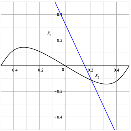
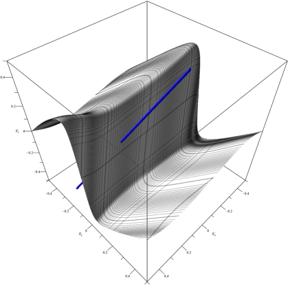
Figure 9: Case $g=2$ (left panel): the image $\mathfrak{u}(z)$, $z\in{\mathbb{R}}\setminus[a_{1},a_{6}]$, of the surface $(\Theta)_{\mathbb{R}}$ (on the square $[-1/2,1/2]^{2}$ with periodic boundary identifications) as per Proposition 7.1. The model problem (4.7) is unsolvable for some $\varkappa_{n}$ if and only if the straight line $W(\varkappa)\in{\mathbb{R}}^{2}\!\!\mod{\mathbb{Z}}^{2}$ (plotted as an example) intersects the plotted curve at $\varkappa=\varkappa_{n}$. Case $g=3$ (right panel): the image of $\pm\int_{a_{1}}^{z_{1}}\vec{\omega}d\zeta\pm\int_{a_{4}}^{z_{2}}\vec{\omega}d\zeta$, $z_{1}\in{\mathbb{R}}\setminus[a_{1},a_{8}]$ and $z_{2}\in[a_{4},a_{5}]$. In blue we plotted an example of the line $W(\varkappa)\in{\mathbb{R}}^{3}\!\!\mod{\mathbb{Z}}^{3}$: the values of $\varkappa$ corresponding to the intersections are the approximate eigenvalues $\varkappa_{n}\sim-\ln\lambda_{n}$. In both cases we have $X_{1}=F(X_{2})$ and $X_{1}=F(X_{2},X_{3})$, respectively, as explained in Lemma 7.5. The line $W(\varkappa)$ is parallel to the (imaginary part of the) first column of the normalized matrix of $B$-periods and intersects the surface by always forming an acute angle with the upward normal (Lemma 7.7).

Lemma 7.5.

Each connected component of the surface $(\Theta)_{\mathbb{R}}$ on the universal covering of $\mathbb{T}_{g}\sim{\mathbb{R}}^{g}$ is smooth. Moreover, it can be expressed as the graph of a function $X_{1}=F(X_{2},\dots X_{g})$, where the function $F:{\mathbb{R}}^{g-1}\to{\mathbb{R}}$ is odd and periodic of period $1$ in each argument.

Proof.

By Proposition 7.1 the points of $(\Theta)_{\mathbb{R}}$ are parametrized by a divisor of $g-1$ points $p_{j}=(z_{j},R_{j})$ chosen arbitrarily in the $A_{j+1}$ cycle ($j=1,\dots,g-1$). Therefore, with notation (7.7),

$$\Theta(\vec{X}(\vec{p})-W_{0})\equiv 0.$$ (7.8)

We want to study the gradient of $\Theta(W-W_{0})$ with respect to $W\in{\mathbb{R}}^{g}$ at the points where $\Theta(W-W_{0})=0$; we notice that since $\Theta$ is periodic on the lattice ${\mathbb{Z}}^{g}$ (A.3), the surface $\Theta(W-W_{0})=0,\ \ W\in{\mathbb{R}}^{g}$ is certainly periodic. To this end we introduce

$$v(z)=\vec{\omega}(z)\cdot\nabla\Theta(W-W_{0}).$$ (7.9)

By Lemma A.8, $v(z)$ is not identically zero and vanishes at the points $p_{j}$ (see Corollary 7.3). Therefore it is of the form

$$v(z)=C\frac{\prod_{j=1}^{g-1}(z-z_{j})}{R(z)}\ ,\ \ C\neq 0.$$ (7.10)

Equations (7.9) and (4.2) (normalization of $\omega_{j}(z)$) imply that

$$\frac{\partial}{\partial W_{s}}\Theta(W-W_{0})=\oint_{A_{s}}v(z)dz,\ \ \ s=1,\dots,g,$$ (7.11)

where $W_{s}$ denotes the $s$-th component of the vector $W\in{\mathbb{R}}^{g}$. In particular, the first component of the gradient of $\Theta$ in (7.11) is given by $C\oint_{A_{1}}\frac{\prod_{j=1}^{g-1}(\zeta-z_{j})d\zeta}{R(\zeta)}$. This expression never vanishes on the surface, because we have established that none of the points $z_{j}$ belongs to $A_{1}$ and thus the integrand has a definite sign. Thus, by the implicit function theorem, it follows that we can express $X_{1}$ as a smooth function $F(X_{2},\dots,X_{g})$ of the remaining components of $\vec{X}$, locally, around any point of the surface and:

$$\frac{\partial X_{1}}{\partial X_{s}}=-\frac{\oint_{A_{s}}\frac{\prod_{j=1}^{g-1}(\zeta-z_{j})d\zeta}{R(\zeta)}}{\oint_{A_{1}}\frac{\prod_{j=1}^{g-1}(\zeta-z_{j})d\zeta}{R(\zeta)}}\in{\mathbb{R}},~{}~{}~{}~{}~{}s=2,\dots,g.$$ (7.12)

We now turn to global injectivity. If there were two $\vec{p}^{(1)},\vec{p}^{(2)}\in A_{2}\times\dots\times A_{g}$ with the same image in the Jacobian under the Abel mapping, then there would exist (by Abel’s theorem) a non-constant and nonzero meromorphic function with at most $g-1$ poles at the points $p^{(1)}_{j}$. But this divisor is non-special (Definition A.7 and following remark) because there is at most one point in each cycle $A_{j}$. This is a contradiction, which proves the required statement.

Thus we have proved that the map $\vec{X}:A_{2}\times\dots\times A_{g}\to\mathbb{T}_{g}$ defines a smooth local function $X_{1}=F(X_{2},\dots X_{g})$ in the neighborhood of any point of the surface. Denote by $\pi_{\widehat{1}}:\mathbb{T}_{g}\to\mathbb{T}_{g-1}$ the projection onto the coordinates $X_{2},\dots,X_{g}$, $\mod{\mathbb{Z}}$: then the assertions proven above imply that $\pi_{\widehat{1}}\circ\vec{X}:A_{2}\times\dots\times A_{g}\to\mathbb{T}_{g-1}$ is a smooth map, in particular it is an open map. Now, $A_{2}\times\dots\times A_{g}$ is a topological space without boundary (meaning that each point is an interior point) and $\pi_{\widehat{1}}\circ\vec{X}$ is smooth and open between two compact spaces. Thus the range of the map cannot have a boundary (by a simple compactness argument) and hence it is surjective. In terms of the universal covering spaces this means that the domain of $F$ is the whole ${\mathbb{R}}^{g-1}$, and therefore, by a compactness argument, $F$ is a global smooth function. Hence for each $N\in{\mathbb{Z}}$ the corresponding connected component of $(\Theta)_{\mathbb{R}}$ is given by $X_{1}=F(X_{2},\dots X_{g})+N$.

Finally we prove the symmetry: since $W_{0}$ is a half-period of the Jacobian, then $\Theta(W-W_{0})=0$ if and only if $\Theta(W+W_{0})=0=\Theta(-W-W_{0})$ (using that $\Theta$ is an even function). Therefore the surface $(\Theta)_{\mathbb{R}}$ is symmetric about the origin, which means that $F(x_{2},\dots x_{g})$ is an odd function. ∎

Remark 7.6.

On the universal covering of $\mathbb{T}_{g}$ (i.e. ${\mathbb{R}}^{g}$) the surface $(\Theta)_{\mathbb{R}}$ is then represented as a countable union of the graphs $X_{1}=F(X_{2},\dots,X_{g})+n$ with $n\in{\mathbb{Z}},X_{2},\dots,X_{g}\in{\mathbb{R}}$.

Lemma 7.7.

(1) The surface $(\Theta)_{\mathbb{R}}$ in $\mathbb{T}_{g}$ is orientable. In particular, there is a continuous choice of normal direction which forms an acute angle with the fixed vector $i{\tau}_{1}$ (see Fig. 9); (2) The intersections of the line $W(\varkappa):{\mathbb{R}}\to\mathbb{T}_{g}$ with $(\Theta)_{\mathbb{R}}$ are transversal and, as a consequence, the zeroes of $\Theta(W(\varkappa)-W_{0})$ as a function of $\varkappa$ are all simple.

Proof.

(1) According to (7.12) a choice of normal direction to the surface $(\Theta)_{\mathbb{R}}$ at the point parametrized by $\vec{p}\in A_{2}\times\dots\times A_{g}$ (see Proposition 7.1) is the vector

$$\vec{n}=\vec{n}(\vec{p})=\left[\oint_{A_{1}}\frac{\prod_{j=1}^{g-1}(\zeta-z_{j})d\zeta}{R(\zeta)},\dots,\oint_{A_{g}}\frac{\prod_{j=1}^{g-1}(\zeta-z_{j})d\zeta}{R(\zeta)}\right]^{t}.$$ (7.13)

Then

$$i\tau_{1}\cdot\vec{n}=i\sum_{j=1}^{g}\oint_{B_{j}}\omega_{1}d\zeta\oint_{A_{j}}\frac{\prod_{j=1}^{g-1}(\zeta-z_{j})d\zeta}{R(\zeta)}.$$ (7.14)

By the Riemann Bilinear Identity ([FK92], equation (3.1.1), p. 64), we have

$$i\tau_{1}\cdot\vec{n}=i\sum_{j=1}^{g}\overbrace{\oint_{A_{j}}\omega_{1}d\zeta}^{=\delta_{1j}}\oint_{B_{j}}\frac{\prod_{j=1}^{g-1}(\zeta-z_{j})d\zeta}{R(\zeta)}=2\sum_{j=2}^{g}\int_{a_{2j-1}}^{a_{2j}}\frac{i\prod_{j=1}^{g-1}(\zeta-z_{j})d\zeta}{R{{}_{+}}(\zeta)}.$$ (7.15)

Each integral in the latter sum is of the same sign. Indeed, on any main arc (branchcut) $R(\zeta)=\sqrt{\prod(\zeta-a_{j})}\in i{\mathbb{R}}$ and the sign of $\Im(R_{+}(\zeta))$ on the main arcs alternates between the neighboring main arcs. The product in the numerator of (7.15) has exactly one zero in the gap in between. Thus, the sign of the (real) integrand in the last term of (7.15) does not change from one main arc $[{a_{2j-1}},a_{2j}]$ to another. Therefore, $i\tau_{1}\cdot\vec{n}\neq 0$ for any point of the surface $(\Theta)_{\mathbb{R}}$ and ${\rm sign}(i\tau_{1}\cdot\vec{n})$ is constant on $(\Theta)_{\mathbb{R}}$.

(2) The surface $(\Theta)_{\mathbb{R}}$ is the zero level surface of $\Theta(z)$ and, therefore, the vector $\nabla\Theta$ is parallel to $\vec{n}$. By part (1), $\nabla\Theta$ cannot be orthogonal to $\frac{d}{d\varkappa}W(\varkappa)=i\tau_{1}$. Now $\Theta$ is an analytic function and the derivative $\frac{d}{d\varkappa}\Theta(W(\varkappa)-W_{0})=\frac{d}{d\varkappa}W(\varkappa)\cdot\nabla\Theta$ does not vanish on $(\Theta)_{\mathbb{R}}$. Thus the zeroes of $\Theta(W(\varkappa)-W_{0})$ are simple. ∎

Corollary 7.8.

The line $W(\varkappa)$ given by (5.4) intersects each connected component of $(\Theta)_{\mathbb{R}}$ in the universal cover exactly once.

Proof.

Consider the function $G(X_{1},\dots,X_{g})=X_{1}-F(X_{2},\dots,X_{g})$, where $F$ is the function whose graph defines the hypersurface $(\Theta)_{\mathbb{R}}$. Then the composite function $G(\vec{W}(\varkappa))$ is strictly monotonic by the transversality of Lemma 7.7. Thus it vanishes exactly once. ∎

The straight line $W(\kappa)$ has slopes $\frac{\tau_{1\ell}}{\tau_{11}}$ and it traverses the fundamental domain from top to bottom with period $\frac{i\pi}{\tau_{11}}$. It should be clear that this line must intersect at least one connected component of $(\Theta)_{\mathbb{R}}$ for each increment $\varkappa\mapsto\varkappa+\frac{i\pi}{\tau_{11}}$.

Theorem 7.9.

Let $X_{1}=F(X_{2},\dots,X_{g-1})+n$ be an equation of the $n$-th connected component of $(\Theta)_{\mathbb{R}}$ (see Lemma 7.5), where $n\in{\mathbb{Z}}$. Then the “maximum excursion” of each connected component of $(\Theta)_{\mathbb{R}}$ in the $X_{1}$ direction is bounded by $g-1$, namely,

$$-\min_{\vec{X}\in{\mathbb{R}}^{g-1}}F(\vec{X})=\max_{\vec{X}\in{\mathbb{R}}^{g-1}}F(\vec{X})\leq\frac{g-1}{2},$$ (7.16)

where $\vec{X}=(X_{2},\dots,X_{g})$.

Proof.

Consider each term in $X_{1}=X_{1}(\vec{z})=\sum_{\ell=1}^{g-1}(\pm)\int_{a_{j_{\ell}}}^{z_{\ell}}\omega_{1}(\zeta)d\zeta$ separately and with the sign that yields a positive contribution. First of all, since our points $z_{\ell}$ are on the real axis, each term is real and, thus, we can consider the real part of $X_{1}$. But then each term is the restriction of the harmonic functions $h_{\ell}(z):=\Re\int_{a_{j_{\ell}}}^{z}\omega_{1}d\zeta$ to a real segment. Each restriction is the same harmonic function up to an additive constant. Each of them is a harmonic function on $\bar{\mathbb{C}}\setminus\bigcup_{j=1}^{3}[a_{2j-1},a_{2j}]$ (harmonic also at $\infty$). Its boundary value on each main arc $[a_{2j-1},a_{2j}]$ is constant and equal to $0$ or $\pm\frac{1}{2}$ (depending on the value of $\ell$). Thus the maximum and minimum of each $h_{\ell}(z)$ on the whole ${\mathbb{C}}\setminus I_{i}\cup I_{e}$ are $\pm\frac{1}{2}$. So, (since the sign on the other sheet is the opposite one) each term can contribute at most a “maximum excursion” of $1/2$. ∎

Remark 7.10.

After extensive numerical investigation we observed that the stronger statement might be true: for any genus $g$, the maximum excursion of each component of the surface $(\Theta)_{\mathbb{R}}$ is at most $1$.

The following corollary provides the bounds on the number $n$ of intersections of the line $W(\varkappa)$, see (5.4), with $(\Theta)_{\mathbb{R}}$ when $\varkappa\in\left[\varkappa_{0},\varkappa_{0}+\frac{N(g-1)i\pi}{\tau_{11}}\right)$, where $\varkappa_{0}>0$ and $N\in{\mathbb{N}}$.

Proposition 7.11.

For any $N\in{\mathbb{N}}$ the number $m(N)$ of intersections of the line $W(\varkappa)$, see (5.4), where $\varkappa\in\left[\varkappa_{0},\varkappa_{0}+\frac{N(g-1)i\pi}{\tau_{11}}\right)$, with $(\Theta)_{\mathbb{R}}$ is bounded by

$$(N-1)(g-1)\leq m(N)\leq(N+1)(g-1).$$ (7.17)

Proof.

The number of different connected components of $({\Theta})$ in the consecutive $N(g-1)$ periods in the $x_{1}$ direction cannot exceed $(N+1)(g-1)$. Now the upper bound follows from Corollary 7.8. On the other hand, any consecutive $N(g-1)$ periods in the $x_{1}$ direction contain at least $(N-1)(g-1)$ different connected components of $({\Theta})$ (that is, these components are completely contained within the aforementioned periods). Using Corollary 7.8 again, we obtain the lower bound in (7.17). ∎

Corollary 7.12.

Let $\varkappa_{n}$ be the $n$-th approximate eigenvalue, that is, the $n$-th zero of

$$\Theta\left(W(\varkappa)-W_{0}\right)=0,$$ (7.18)

where $W(\varkappa)$ and $W_{0}$ are defined by (5.4) and the labelling of solutions of (7.18) fixed by Remark 5.10. Let $2\lambda_{n}=e^{-\varkappa_{n}+\ln 2}$ denote the corresponding approximate singular values. Then

$$\varkappa_{n}=n\pi\frac{i}{{\tau}_{11}}+O(1),~{}~{}~{}~{}~{}~{}~{}~{}~{}\qquad\lambda_{n}=e^{-n\pi\frac{i}{{\tau}_{11}}+O(1)}.$$ (7.19)

The proof of Corollary 7.12 follows from (5.4) and Proposition 7.11. Combined with Corollary 6.3, Corollary 7.12 yields the following result.

Theorem 7.13.

Let $\varkappa^{exact}_{n}$ be the $n$-th exact eigenvalue of the RHP (3.10), see Definition 5.9, and let $2\lambda^{exact}_{n}=e^{-\varkappa^{exact}_{n}+\ln 2}$ denote the corresponding singular values of ${\mathcal{H}}^{-1}_{e}$. Then

$$\varkappa^{exact}_{n}=n\pi\frac{i}{{\tau}_{11}}+O(1),~{}~{}~{}~{}~{}~{}~{}~{}~{}\qquad 2\lambda^{exact}_{n}=e^{-n\pi\frac{i}{{\tau}_{11}}+O(1)}.$$ (7.20)

7.1 Comparison with the two-interval (genus 1) case

We would like to compare the one interior and two exterior interval case (i.e. $g=2$ in (1.1)–(1.3)) with the corresponding asymptotics in the two interval (four-point) case ($I_{e}=[a_{1},a_{2}]$, $I_{i}=[a_{3},a_{4}]$). The latter is obtained from the former in the limit when the rightmost exterior interval $[a_{5},a_{6}]$ collapses into a point $a$ as $a_{5}=a-\epsilon,~{}a_{6}=a+\epsilon$ with $\epsilon\rightarrow 0^{+}$. The singular values of the FHT (with no weight) in the four point case was studied in [KT12]. Since the weight $w(z)$ affects only $d(z)$, but not ${\mathfrak{g}}(z)$, see (4.25), the leading large $\varkappa$ asymptotics of singular values for both FHTs remains the same. According to (5.1), (4.3), (4.12) and (4.12) (for $g=2$)

$$\begin{split}{\tau}_{11}&=[1,0]\mathbb{A}^{-1}\oint_{\hat{\gamma}_{1}}\left[\begin{matrix}1\\ \zeta\end{matrix}\right]\frac{d\zeta}{R(\zeta)}=[1,0]\left[\begin{array}[]{cc}1&-1\\ 0&1\end{array}\right]\dfrac{\left[\begin{array}[]{c c c }\int_{c_{2}}\frac{\zeta d\zeta}{R(\zeta)}&-\int_{c_{2}}\frac{d\zeta}{R(\zeta)}\\ -\int_{c_{1}}\frac{\zeta d\zeta}{R(\zeta)}&\int_{c_{1}}\frac{d\zeta}{R(\zeta)}\end{array}\right]\left[\begin{matrix}\int_{\gamma_{1}}\frac{d\zeta}{R(\zeta)}\\ \int_{\gamma_{1}}\frac{\zeta d\zeta}{R(\zeta)}\end{matrix}\right]}{\left|\begin{array}[]{c c c }\int_{c_{1}}\frac{d\zeta}{R(\zeta)}&\int_{c_{2}}\frac{d\zeta}{R(\zeta)}\\ \int_{c_{1}}\frac{\zeta d\zeta}{R(\zeta)}&\int_{c_{2}}\frac{\zeta d\zeta}{R(\zeta)}\end{array}\right|}\\ &=\frac{\int_{c_{2}\cup c_{1}}\frac{\zeta d\zeta}{R(\zeta)}\int_{\gamma_{1}}\frac{d\zeta}{R(\zeta)}-\int_{c_{2}\cup c_{1}}\frac{d\zeta}{R(\zeta)}\int_{\gamma_{1}}\frac{\zeta d\zeta}{R(\zeta)}}{\int_{c_{2}}\frac{\zeta d\zeta}{R(\zeta)}\int_{c_{1}}\frac{d\zeta}{R(\zeta)}-\int_{c_{2}}\frac{d\zeta}{R(\zeta)}\int_{c_{1}}\frac{\zeta d\zeta}{R(\zeta)}}=\dfrac{\left|\begin{array}[]{c c c }\int_{\gamma_{1}}\frac{d\zeta}{R(\zeta)}&\int_{c_{1}\cup c_{2}}\frac{d\zeta}{R(\zeta)}\\ \int_{\gamma_{1}}\frac{\zeta d\zeta}{R(\zeta)}&\int_{c_{1}\cup c_{2}}\frac{\zeta d\zeta}{R(\zeta)}\end{array}\right|}{\left|\begin{array}[]{c c c }\int_{c_{1}}\frac{d\zeta}{R(\zeta)}&\int_{c_{2}}\frac{d\zeta}{R(\zeta)}\\ \int_{c_{1}}\frac{\zeta d\zeta}{R(\zeta)}&\int_{c_{2}}\frac{\zeta d\zeta}{R(\zeta)}\end{array}\right|}.\end{split}$$ (7.21)

Since ${\tau}_{11}$ is the ratio of two determinants, we can replace $\zeta d\zeta$ in the numerators of the second rows of each determinant by $(\zeta-a)d\zeta$. Let us calculate the limits of $\int_{c_{2}}\frac{(\zeta-a)^{k}d\zeta}{R(\zeta)}$, where $k=0,1$, as $\epsilon\rightarrow 0^{+}$. First note that

$$R(\zeta)=R_{0}(\zeta)\sqrt{(\zeta-a)^{2}-\epsilon^{2}},$$ (7.22)

where $R_{0}(\zeta)=\prod_{j=1}^{4}(\zeta-a_{j})^{\frac{1}{2}}$ is an analytic function near $\zeta=a$. Because of the shrinking interval $\gamma_{2}$, the large contribution to the integrals over the complementary arc $c_{2}$ may come only from a neighborhood of $a$. Replacing this integral with the integral over the corresponding cycle on the Riemann surface $\mathcal{R}$, we obtain

$$\int_{c_{2}}\frac{(\zeta-a)^{k}d\zeta}{R(\zeta)}=-\frac{1}{2}\left(\int_{a}^{a+ir}+\int_{a}^{a-ir}\right)\frac{(\zeta-a)^{k}d\zeta}{R(\zeta)}+O(1)$$ (7.23)

as $\epsilon\rightarrow 0$, where $r>0$ is a fixed number. Notice that for any $k\in{\mathbb{R}}^{+}$ the integrals in the right hand side of (7.23) are bounded. Indeed, $R_{0}(\zeta)$ is bounded and

$$\left|\frac{(\zeta-a)^{k}}{\sqrt{(\zeta-a)^{2}-\epsilon^{2}}}\right|\leq|\zeta-a|^{k-1}\qquad{\rm when}~{}~{}~{}~{}\zeta\in[a-ir,a+ir].$$ (7.24)

In the remaining case $k=0$, we start with the Taylor formula $[R(\zeta)]^{-1}=[R(a)]^{-1}+(\zeta-a)(R^{-1})^{\prime}(\eta)$, where $\eta\in(\zeta,a)$. Since $(R^{-1})^{\prime}(\zeta)$ is bounded on $[a-ir,a+ir]$, we can rewrite (7.23) as

$$\begin{split}\int_{c_{2}}\frac{d\zeta}{R(\zeta)}&=-\frac{1}{2R_{0}(a)}\left(\int_{a}^{a+ir}+\int_{a}^{a-ir}\right)\frac{d\zeta}{\sqrt{(\zeta-a)^{2}-\epsilon^{2}}}+O(1)\\ &=-\frac{1}{2R_{0}(a)}\left(\int_{0}^{\frac{ir}{\epsilon}}+\int_{0}^{-\frac{ir}{\epsilon}}\right)\frac{dt}{\sqrt{t^{2}-1}}+O(1)=\frac{\ln\epsilon}{R_{0}(a)}+O(1).\end{split}$$ (7.25)

Now, according to (7.21) and (7.25), $\displaystyle\lim_{\epsilon\rightarrow 0}{\tau}_{11}=\lim_{\epsilon\rightarrow 0}\frac{\int_{\gamma_{1}}\frac{(\zeta-a)d\zeta}{R(\zeta)}}{\int_{c_{1}}\frac{(\zeta-a)d\zeta}{R(\zeta)}}=\frac{\int_{\gamma_{1}}\frac{d\zeta}{R_{0}(\zeta)}}{\int_{c_{1}}\frac{d\zeta}{R_{0}(\zeta)}}$. So,

$$2\lambda_{n}=e^{-n\pi\frac{\int_{c_{1}}\frac{d\zeta}{R_{0}(\zeta)}}{\int_{\gamma_{1}}\frac{d\zeta}{iR_{0}(\zeta)}}+O(1)},$$ (7.26)

which coincides with the corresponding expression from [KT12].

7.2 Asymptotics of Eigenfunctions

Let $\varkappa_{n}$ be the $n$-th approximate eigenvalue. Then $\Theta(W(\varkappa_{n})-W_{0})=0$. If $\mathbf{f}_{n}:=W(\varkappa_{n})-W_{0}$ then, according to Theorem A.5, $\mathbf{f}_{n}=\sum_{j=1}^{g-1}\mathfrak{u}(p_{j})+\mathcal{K}$, where the points $p_{j}=(z_{j},R_{j})$, discussed in Proposition 7.1, belong to the cycles $A_{j+1}$ of the Riemann surface. For this reason it makes sense to consider ${\bf f}(\vec{p}):=\sum_{j=1}^{g-1}\mathfrak{u}(p_{j})+\mathcal{K}$, where $\vec{p}=(p_{1},\dots,p_{g-1})$, as a function on the (universal cover) of the torus $A_{2}\times\dots A_{g}$, so that ${\bf f}_{n}={\bf f}(\vec{p}_{n})$ for some points $\vec{p}_{n}\in A_{2}\times\dots A_{g}$.

Lemma 7.14.

(1) For $\Psi(z;\varkappa)$ from Theorem 5.7 we have

$$\mathop{\mathrm{res}}\limits_{\varkappa=\varkappa_{n}}\Psi(z;\varkappa)=C_{0}\left[\begin{matrix}\displaystyle\frac{i\pi\Theta\left(\mathfrak{u}(z)-\mathfrak{u}(\infty)+{\bf f}(\vec{p}_{n})\right)h(z)}{\vec{\tau}_{1}\!\!\cdot\!\!\nabla\Theta({\bf f}(\vec{p}_{n}))\Theta\left(\mathfrak{u}(z)-\mathfrak{u}(\infty)+W_{0}\right)}&\displaystyle\frac{i\pi\Theta\left(-\mathfrak{u}(z)-\mathfrak{u}(\infty)+{\bf f}(\vec{p}_{n})\right)h(z)}{\vec{\tau}_{1}\!\!\cdot\!\!\nabla\Theta({\bf f}(\vec{p}_{n}))\Theta\left(-\mathfrak{u}(z)-\mathfrak{u}(\infty)+W_{0}\right)}\\[21.52771pt] \displaystyle\frac{-i\pi\Theta\left(\mathfrak{u}(z)+\mathfrak{u}(\infty)+{\bf f}(\vec{p}_{n})\right)h(z)}{\vec{\tau}_{1}\!\!\cdot\!\!\nabla\Theta({\bf f}(\vec{p}_{n}))\Theta\left(\mathfrak{u}(z)+\mathfrak{u}(\infty)+W_{0}\right)}&\displaystyle\frac{-i\pi\Theta\left(-\mathfrak{u}(z)+\mathfrak{u}(\infty)+{\bf f}(\vec{p}_{n})\right)h(z)}{\vec{\tau}_{1}\!\!\cdot\!\!\nabla\Theta({\bf f}(\vec{p}_{n}))\Theta\left(-\mathfrak{u}(z)+\mathfrak{u}(\infty)+W_{0}\right)}\end{matrix}\right].$$ (7.27)

${\bf(2)}$ For any $\vec{p}_{n}\in A_{2}\times\dots\times A_{g}$ the matrix is not identically zero. (3) The two rows are proportional to each other for any $\vec{p}_{n}\in A_{2}\times\dots\times A_{g}$.

Proof.

(1) Expression (7.27) follows directly from Theorem 5.7.

(2) Let $\vec{p}$ be an arbitrary point on $A_{2}\times\dots A_{g}$. It was proven in Lemma 7.7, (1), that $\vec{\tau}_{1}\cdot\nabla\Theta({\bf f}(\vec{p}))\neq 0$. Similarly the other Theta functions in the denominators cannot be identically zero functions of $z$ because the degree $g$ divisors $\sum_{j=1}^{g-1}p_{j}+\infty_{1,2}$ are non-special as well. The only expressions that may be identically zero are the Theta functions $\Theta(\pm\mathfrak{u}(z)\pm\mathfrak{u}(\infty)+{\bf f}(\vec{p}_{n}))$. According to the Riemann theorem ([FK92], p. 317) this happens if and only if ${\bf f}(\vec{p})\pm\mathfrak{u}(\infty)-\mathcal{K}=\sum_{j=1}^{g-1}\mathfrak{u}(p_{j})\pm\mathfrak{u}(\infty)$ is a special divisor of degree $g$. According to the description of special divisors (see after Definition A.7) this happens only if there is a pair of points with the same $z$–coordinate. By inspection we see that this happens if and only if $p_{g-1}\in A_{g}$ lies above $z=\infty$ in such a way that $\mathfrak{u}(p_{g-1})\pm\mathfrak{u}(\infty)=0$ (i.e. on the secondary sheet in the case of the $+$ sign and on the main sheet in the case of the $-$ sign). For example, if $p_{g-1}=\infty_{1}$ (the infinity on the main sheet), then the whole first row of (7.27) vanishes; but in that case the second row is not identically vanishing because $\sum_{j=1}^{g-1}\mathfrak{u}(p_{j})+\mathfrak{u}(\infty_{2})$ is a non-special divisor of degree $g$ (and thus the entries of the second row vanish only at $g$ points of the Riemann surface). Similarly, if $p_{g-1}=\infty_{2}$, the second row vanishes, but the first one does not.

(3) We now address the linear dependence of the rows of (7.27) as a function of $\vec{p}=\vec{p}_{n}\in A_{2}\times\dots\times A_{g}$. First of all we see that ${\bf f}(\vec{p})$ changes by integer valued vectors as $\vec{p}$ winds around the torus $A_{2}\times\dots A_{g}$. Since $\Theta$-function is (strictly) periodic in ${\mathbb{Z}}^{g}$, the right hand side of (7.27) is a well–defined function of $\vec{p}$ on the torus $A_{2}\times\dots A_{g}$. Now, of course, we can assume without loss of generality that both rows are non identically zero (in $z$) (if one of them is identically zero there is nothing else to prove). Consider the ratio of $(1,1)$ and $(2,1)$ entries of (7.27)

$$-\frac{\Theta\left(\mathfrak{u}(z)-\mathfrak{u}(\infty)+{\bf f}(\vec{p})\right)}{\Theta\left(\mathfrak{u}(z)-\mathfrak{u}(\infty)+W_{0}\right)}\frac{\Theta\left(\mathfrak{u}(z)+\mathfrak{u}(\infty)+W_{0}\right)}{\Theta\left(\mathfrak{u}(z)+\mathfrak{u}(\infty)+{\bf f}(\vec{p})\right)}\ .$$ (7.28)

Using the periodicity of the $\Theta$-functions (A.3) and the jump relations for $\mathfrak{u}(z)$ in Proposition 5.4, the reader can verify that the above expression does not have jumps across the real axis, and therefore defines a rational function. In fact the denominator can vanish at most at $g$ points by Theorem A.3. The zeroes of the numerator are at $\infty_{1,2}$ (on the two sheets), at the points $a_{j}{,\ j\in J}=\{1,5,7,9...,2g-1\}$ (see Proposition 7.1) and at the points $\widehat{p}_{1},\dots,\widehat{p}_{g-1}$ (recall, $\widehat{}$ denotes the sheet exchange); both these statements follow from the explicit form of $W_{0}$ in (5.19), the definition of ${\bf f}(\vec{p})$ and from Theorem A.3. The denominator has zeroes at the same points and thus the ratio is constant. In a similar way, one can verify that the ratio of the $(1,2)$ and $(2,2)$ entries of (7.27) is also a constant:

$$-\frac{\Theta\left(-\mathfrak{u}(z)-\mathfrak{u}(\infty)+{\bf f}(\vec{p})\right)}{\Theta\left(-\mathfrak{u}(z)-\mathfrak{u}(\infty)+W_{0}\right)}\frac{\Theta\left(-\mathfrak{u}(z)+\mathfrak{u}(\infty)+W_{0}\right)}{\Theta\left(-\mathfrak{u}(z)+\mathfrak{u}(\infty)+{\bf f}(\vec{p})\right)}.$$ (7.29)

Indeed one verifies that the expression (7.29) has no jumps and thus is a rational function; now both the numerator and denominator vanish at $\infty_{1,2},p_{1},\dots,p_{g-1}$. Evaluating, for example, at $z=a_{1}$ where $\mathfrak{u}(a_{1})=0$ shows that (7.28) and (7.29) are the same constant. ∎

According to Proposition 3.19, we can now proceed to the evaluation of the approximation to the eigenfunctions of the operator $\widehat{K}$.

Theorem 7.15.

Let $\varkappa_{n}$ be the $n$-th approximate eigenvalue and $n$ sufficiently large. Then, uniformly in each closed subset of $I=I_{i}\cup I_{e}$ not containing any endpoints $a_{l},~{}l=1,2\dots,2g+2$, we have the approximation of the eigenfunctions of $\widehat{K}$ given by either of the expressions

$$\begin{split}&\phi_{n,j}(z)={(-1)^{j}}2{\rm e}^{(-1)^{j+1}(d_{\infty}+\varkappa_{n}{\mathfrak{g}}_{\infty})-\frac{\varkappa_{n}}{2}}\\ &\times\left\{\Re\left[\frac{\pi C_{0}\Theta\left(\mathfrak{u}_{+}(z)+(-1)^{j}\mathfrak{u}(\infty)+{\bf f}(\vec{p}_{n})\right)h_{+}(z)}{{i}\vec{\tau}_{1}\!\!\cdot\!\!\nabla\Theta({\bf f}(\vec{p}_{n}))\Theta\left(\mathfrak{u}_{+}(z)+(-1)^{j}\mathfrak{u}(\infty)+W_{0}\right)}{\rm e}^{-i\Im(d_{+}(z))-i\varkappa_{n}\Im({\mathfrak{g}}_{+}(z))}\right]\chi_{e}\right.\\ &\hskip 10.0pt\left.+i\Im\left[\frac{\pi C_{0}\Theta\left(\mathfrak{u}_{+}(z)+(-1)^{j}\mathfrak{u}(\infty)+{\bf f}(\vec{p}_{n})\right)h_{+}(z)}{{i}\vec{\tau}_{1}\!\!\cdot\!\!\nabla\Theta({\bf f}(\vec{p}_{n}))\Theta\left(\mathfrak{u}_{+}(z)+(-1)^{j}\mathfrak{u}(\infty)+W_{0}\right)}{\rm e}^{-i\Im(d_{+}(z))-i\varkappa_{n}\Im({\mathfrak{g}}_{+}(z))}\right]\chi_{i}+\mathcal{O}(\varkappa_{n}^{-1})\right\},\end{split}$$ (7.30)

$j=1,2$, where the (independent on $n$) constants $W_{0},C_{0}$ and function $h$ were defined in (5.4), (5.44) and (5.27), provided that these expressions are not identically zero. In this case, the expressions in the right hand side of (7.30) are proportional to each other by a nonzero constant in $z$. If one of the two expressions is identically zero for a particular value of $n$, then the other expression is not identically zero.

Proof.

Unraveling all the steps that transformed the RHP 3.10 to its final approximation, we have in summary:

• On any closed set in ${\mathbb{C}}\setminus{I}$

  $$\Gamma(z;\lambda)={\rm e}^{(d_{\infty}+\varkappa{\mathfrak{g}}_{\infty}){\sigma}_{3}}\mathcal{E}\Psi{\rm e}^{-d{\sigma}_{3}}{\rm e}^{-\varkappa{\mathfrak{g}}{\sigma}_{3}},$$ (7.31)

  where $\mathcal{E}(z)$ is the error matrix, which differs from the identity (uniformly) by an $\mathcal{O}(\varkappa^{-1})$, $\varkappa\to\infty$, term, and $\Psi$ is the solution to the RHP 4.7;

• The boundary values of $\Gamma$ in the interior/exterior intervals in terms of our approximation are read off from (4.32) and (4.25):

  $$\Gamma_{\pm}(z;\lambda)={\rm e}^{(d_{\infty}+\varkappa{\mathfrak{g}}_{\infty}){\sigma}_{3}}\mathcal{E}\Psi_{\pm}{\rm e}^{-d_{\pm}{\sigma}_{3}}\left[\begin{matrix}1&\displaystyle\pm\frac{{\rm e}^{-\varkappa(2{\mathfrak{g}}_{\pm}+1)}}{iw}\chi_{{}_{i}}\\ \displaystyle\pm iw{\rm e}^{\varkappa(2{\mathfrak{g}}_{\pm}-1)}\chi_{{}_{e}}&1\end{matrix}\right]{\rm e}^{-\varkappa{\mathfrak{g}}_{\pm}{\sigma}_{3}},\,z\in I.$$ (7.32)

Using formula (3.30) (with $\lambda=e^{-\varkappa}$), we can approximate $\varphi_{j}(z;\lambda)$. Referring now to (3.30), we point out that $A_{j}(z;\lambda)$ is analytic on $I_{e}$, and $B_{j}(z;\lambda)$ is analytic on $I_{i}$. Therefore we can use either the $+$ or $-$ boundary values of $\Psi$ when we approximate $\varphi_{j}(z;\lambda)$ in terms of $\Psi$. Using, for example, the $+$ boundary value, we find that for $z\in I$ one has:

$$\begin{split}&\varphi_{j}(z;\lambda)=\frac{{\rm e}^{(-1)^{j+1}(d_{\infty}+\varkappa{\mathfrak{g}}_{\infty})}}{\sqrt{w(z)}}\left[\Psi_{j1+}{\rm e}^{-d_{+}-\varkappa{\mathfrak{g}}_{+}}+iw{\rm e}^{\varkappa{\mathfrak{g}}_{+}-\varkappa+d_{+}}\Psi_{j2+}+\mathcal{O}(\varkappa^{-1})\right]\chi_{e}\\ &\quad+i\sqrt{w(z)}{\rm e}^{(-1)^{j+1}(d_{\infty}+\varkappa{\mathfrak{g}}_{\infty})}\left[\frac{\Psi_{j1+}}{iw}{\rm e}^{-\varkappa{\mathfrak{g}}_{+}-\varkappa-d_{+}}+\Psi_{j2+}{\rm e}^{\varkappa{\mathfrak{g}}_{+}+d_{+}}+\mathcal{O}(\varkappa^{-1})\right]\chi_{i}\\ =&{\rm e}^{(-1)^{j+1}(d_{\infty}+\varkappa{\mathfrak{g}}_{\infty})-\frac{\varkappa}{2}}\left[\Psi_{j1+}{\rm e}^{-\frac{d_{+}-d_{-}}{2}-\varkappa\frac{{\mathfrak{g}}_{+}-{\mathfrak{g}}_{-}}{2}}+{\rm e}^{\varkappa\frac{{\mathfrak{g}}_{+}-{\mathfrak{g}}_{-}}{2}+\frac{d_{+}-d_{-}}{2}}\Psi_{j1-}+\mathcal{O}(\varkappa^{-1})\right]\chi_{e}\\ +&{{\rm e}^{(-1)^{j+1}(d_{\infty}+\varkappa{\mathfrak{g}}_{\infty})-\frac{\varkappa}{2}}}\left[\Psi_{j1+}{\rm e}^{-\varkappa\frac{{\mathfrak{g}}_{+}-{\mathfrak{g}}_{-}}{2}-\frac{d_{+}-d_{-}}{2}}-\Psi_{j1-}{\rm e}^{\varkappa\frac{{\mathfrak{g}}_{+}-{\mathfrak{g}}_{-}}{2}+\frac{d_{+}-d_{-}}{2}}+\mathcal{O}(\varkappa^{-1})\right]\chi_{i}.\end{split}$$ (7.33)

We have used the jump conditions in RHP 4.7 in (7.33) and the properties (4.5) of ${\mathfrak{g}}$. In order to compute the eigenfunctions of $\widehat{K}$ we need to take the residue of (7.33) according to Proposition 3.19 at the eigenvalues $\lambda_{n}={\rm e}^{-\varkappa_{n}^{exact}}$ with respect to $\varkappa$ (since $\frac{d\lambda}{\lambda}=-d\varkappa$) so that we need to use (7.27). Given that the approximation (7.33) is uniform in a strip around the positive real $\varkappa$–axis, the process of taking residues does not affect the error term. We also recall that $\Psi_{j1-}=\overline{\Psi_{j1+}}$, see Proposition 4.8, and the same applies to the residues at $\varkappa_{n}\in{\mathbb{R}}$. Moreover, it follows from (4.4) and (4.19), respectively, that ${\mathfrak{g}}_{+}-{\mathfrak{g}}_{-}=2i\Im{\mathfrak{g}}_{+}$ and $d_{+}-d_{-}=2i\Im d_{+}$ on the main arcs. Thus we obtain (7.30). Note also that, according to assertion (2) of Lemma 7.14, at least one of $\phi_{n,j}$, $j=1,2$, is not identically zero. Moreover, assertion (3) of Lemma 7.14 implies that if both $\phi_{n,j}$, $j=1,2$ are nonzero functions, then they are multiple of each other. ∎

In order to provide the approximation of the normalized eigenfunctions for $\widehat{K}$ we need to compute the norms of the approximate eigenfunctions from Theorem 7.15.

Lemma 7.16.

(1) The following identities hold for $j=1,2$:

$$N_{j}(\vec{p}_{n}) :=-\frac{i}{\pi^{2}}\oint_{B_{1}}\mathop{\mathrm{res}}\limits_{\varkappa=\varkappa_{n}}\!\!\!\Psi_{j1}(z;\varkappa)\!\!\!\mathop{\mathrm{res}}\limits_{\varkappa=\varkappa_{n}}\!\!\!\Psi_{j2}(z;\varkappa)dz=$$ (7.35)

$$=\frac{\Theta({\mathbf{f}}(\vec{p}_{n})+(-1)^{j}2\mathfrak{u}(\infty))}{\Theta(W_{0}+(-1)^{j}2\mathfrak{u}(\infty))}\frac{[\mathbb{A}^{-1}\nabla\Theta(W_{0})]_{g}}{i\vec{\tau}_{1}\!\!\cdot\!\!\nabla\Theta({\mathbf{f}}(\vec{p}_{n}))}.$$

(2) The function $N_{j}(\vec{p})$ is a real analytic function of $\vec{p}\in A_{2}\times\dots\times A_{g}$. It vanishes to second order at $p_{g-1}=\infty_{l}$, where $\infty_{l}$ is the point at $z=\infty$ on the sheet $l=1,2$, and has no other zeroes.

Proof.

(1) First notice that the ratios in (7.35) are well-defined because $\Theta(W_{0}+(-1)^{j}2\mathfrak{u}(\infty))\neq 0$ (third bullet point of Lemma 5.5) and ${\nabla}\Theta(\mathbf{f}(\vec{p}_{n}))\neq 0$ ( Lemma 7.7). Using the expressions for $\Psi_{ij}$ from (7.27), we obtain

$$\ \ \ \ \ \ -i\oint_{B_{1}}\mathop{\mathrm{res}}\limits_{\varkappa=\varkappa_{n}}\!\!\!\Psi_{j1}(z;\varkappa)\!\!\!\mathop{\mathrm{res}}\limits_{\varkappa=\varkappa_{n}}\!\!\!\Psi_{j2}(z;\varkappa)dz=\frac{-iC_{0}^{2}\pi^{2}}{(\vec{\tau}_{1}\!\!\cdot\!\!\nabla\Theta(\mathbf{f}(\vec{p}_{n})))^{2}}\times$$ (7.36)

$$\times\oint_{B_{1}}\!\!\!\!\frac{\Theta(\mathfrak{u}(z)+(-1)^{j}\mathfrak{u}(\infty)+\mathbf{f}(\vec{p}_{n}))\Theta(-\mathfrak{u}(z)+(-1)^{j}\mathfrak{u}(\infty)+\mathbf{f}(\vec{p}_{n}))h^{2}(z)dz}{\Theta(\mathfrak{u}(z)+(-1)^{j}\mathfrak{u}(\infty)+W_{0})\Theta(-\mathfrak{u}(z)+(-1)^{j}\mathfrak{u}(\infty)+W_{0})}.$$

Now the integrand is a differential with no poles (the finite zeroes in the denominator cancel with those of $h^{2}$ by construction of $W_{0}$, and the zeroes at $\infty$ cancel with those in the numerator). The numerator also vanishes at the points $z=p_{j}^{(n)}$ of the components of ${\vec{p}_{n}}=(p_{1}^{(n)},\dots,p_{g-1}^{(n)})$ and their reflections on the opposite sheet; in other words it is a holomorphic differential of the form $\propto\frac{\prod_{j=1}^{g-1}(z-z_{j}^{(n)})}{R(z)}dz$. Here $z_{j}^{(n)}$ are the $z$–coordinates of the points $p_{j}^{(n)}$. As such, the differential must be proportional to $\vec{\omega}(z)\cdot\nabla\Theta(\mathbf{f}(\vec{p}_{n}))dz$ (Lemma A.8). To decide the proportionality constant it suffices to evaluate the two expressions at $\infty$, so one finds

$$\frac{\Theta(\mathfrak{u}(z)+(-1)^{j}\mathfrak{u}(\infty)+\mathbf{f}_{n})\Theta(-\mathfrak{u}(z)+(-)^{j}\mathfrak{u}(\infty)+\mathbf{f}_{n})h^{2}(z)}{\Theta(\mathfrak{u}(z)+(-1)^{j}\mathfrak{u}(\infty)+W_{0})\Theta(-\mathfrak{u}(z)+(-1)^{j}\mathfrak{u}(\infty)+W_{0})}=$$

$$=\frac{\Theta(\mathbf{f}_{n}+(-1)^{j}2\mathfrak{u}(\infty))}{C_{0}\Theta(W_{0}+(-1)^{j}2\mathfrak{u}(\infty))}\vec{\omega}(z)\cdot\nabla\Theta(\mathbf{f}_{n}),$$

and the right-hand side of (7.36) becomes

$$\frac{-i\Theta(\mathbf{f}_{n}+(-1)^{j}2\mathfrak{u}(\infty))}{\Theta(W_{0}+(-1)^{j}2\mathfrak{u}(\infty))}\frac{C_{0}\pi^{2}}{(\vec{\tau}_{1}\!\!\cdot\!\!\nabla\Theta(\mathbf{f}_{n}))^{2}}\oint_{B_{1}}\vec{\omega}(z)\cdot\nabla\Theta(\mathbf{f}_{n})=$$ (7.37)

$$=\frac{\Theta(\mathbf{f}_{n}+(-1)^{j}2\mathfrak{u}(\infty))}{\Theta(W_{0}+(-1)^{j}2\mathfrak{u}(\infty))}\frac{C_{0}\pi^{2}}{i\vec{\tau}_{1}\!\!\cdot\!\!\nabla\Theta(\mathbf{f}_{n})}.$$ (7.38)

Thus, recalling formula (5.44) for $C_{0}$ completes the proof. (2) It can be shown using the periodicity of $\Theta$ and the Schwarz symmetry that $N_{j}(\vec{p})$ is real–valued when $\vec{p}\in A_{2}\times\dots\times A_{g}$. According to Corollary A.5, the term $\Theta({\bf f}(\vec{p})+(-1)^{j}2\mathfrak{u}(\infty))$ in (7.35) vanishes on $A_{2}\times\dots A_{g}$ if and only if the point $p_{g-1}\in A_{g}$ coincides with $\infty_{j}$, see Figure 6. To prove that the vanishing is of second order, consider the case $j=1$ for definiteness:

$${\bf f}(\vec{p})-2\mathfrak{u}(\infty)=\mathfrak{u}(p_{g-1})+\sum_{j=1}^{g-2}\mathfrak{u}(p_{j})-2\mathfrak{u}(\infty)-\mathcal{K}=\mathfrak{u}(p_{g-1})-\left(\sum_{j=1}^{g-2}\mathfrak{u}(\widehat{p}_{j})+2\mathfrak{u}(\infty)\right)+\mathcal{K},$$ (7.39)

where the equalities are in the Jacobian and we have used the fact that $\mathcal{K}=-\mathcal{K}$ in the Jacobian Then, by Theorem A.3, $\Theta({{\bf f}(\vec{p})}-2\mathfrak{u}(\infty))$ has a second order zero at $p_{g-1}=\infty$ on the main sheet. ∎

Corollary 7.17.

The functions $N_{j}(\vec{p})$ have constant sign on the torus $A_{2}\times\dots A_{g}$. The function $\sqrt{N_{j}(\vec{p})}$ can be defined analytically on the double cover of $A_{2}\times\dots A_{g}$.

Proof.

By Lemma 7.16, (2), $N_{j}(\vec{p})$ are real and vanish quadratically at $p_{g-1}=\infty_{j}$ and thus the square root can be analytically continued across the hypersurface $p_{g-1}=\infty_{j}$. Since this is the only sign change on the cycle $p_{g-1}\in A_{g}$, we conclude that $\sqrt{N_{j}(\vec{p})}$ gains the opposite sign under the analytic continuation in the variable $p_{g-1}\in A_{g}$. Thus, it is well-defined on the double cover of the $A_{g}$ component. ∎

Remark 7.18.

Although it is nontrivial to prove it directly using properties of the Theta functions, it will follow from the Proposition 7.19 below that $N_{j}(\vec{p})$ is actually positive since it appears in (7.40) as an approximation of a positive quantity (norm).

Proposition 7.19.

(1) The norms in $L^{2}({I})$ of the eigenfunctions $\phi_{n,j}$ appearing in Theorem 7.15, are

$$\|\phi_{n,j}\|^{2}=2{\rm e}^{(-1)^{j+1}2(d_{\infty}+\varkappa_{n}{\mathfrak{g}}_{\infty})-\varkappa_{n}}\left(\pi^{2}N_{j}(\vec{p}_{n})+\mathcal{O}(\varkappa_{n}^{-1})\right),~{}~{}~{}j=1,2.$$ (7.40)

(2) There exists $\nu>0$ such that for all $n\in{\mathbb{N}}$

$$\max_{j=1,2}|N_{j}(\vec{p}_{n})|>\nu.$$ (7.41)

Proof.

(1) We will, for concreteness, consider $j=1$ (i.e., the first row in (7.27)). First of all, recall that by Proposition 3.19, $\phi_{n,1}(z)$ is related to $\Gamma(z;\lambda)$. Thus its squared norm in $L^{2}(I_{e}\sqcup I_{i})$ is the sum of the two pieces on $I_{i}$ and $I_{i}$. Since the eigenfunctions are the residues of $\Gamma(z;\lambda)$ as per Proposition 3.19, we need to compute the expressions below (where $J(H):=H_{+}-H_{-}$):

$$\begin{split}\int_{I_{e}}|\phi_{n,1}|^{2}dz&=\int_{I_{e}}\left(\mathop{\mathrm{res}}\limits_{\lambda=\lambda_{n}}\Gamma_{11}(z;\lambda)\frac{1}{\lambda}\right)^{2}\frac{dz}{w(z)}=\cr&=\int_{I_{e}}\left(\mathop{\mathrm{res}}\limits_{\lambda=\lambda_{n}}\Gamma_{11}(z;\lambda)\frac{1}{\lambda}\right)\left(\mathop{\mathrm{res}}\limits_{\lambda=\lambda_{n}}i\lambda J(\Gamma_{12}(z;\lambda))\frac{1}{\lambda}\right)dz=\\ &=i\left(\oint_{B_{0}}+\oint_{B_{g}}\right)\mathop{\mathrm{res}}\limits_{\lambda=\lambda_{n}}\left(\Gamma_{11}(z;\lambda)\frac{1}{\lambda}\right)\mathop{\mathrm{res}}\limits_{\lambda=\lambda_{n}}\left(\Gamma_{12}(z;\lambda)\right)dz;\end{split}$$ (7.42)

$$\begin{split}\int_{I_{i}}|\phi_{n,1}|^{2}dz&=\int_{I_{i}}\left(\mathop{\mathrm{res}}\limits_{\lambda=\lambda_{n}}\Gamma_{12}(z;\lambda)\frac{1}{\lambda}\right)^{2}\!\!\!\!{w(z)}dz=\\ &=-i\int_{I_{i}}\left(\mathop{\mathrm{res}}\limits_{\lambda=\lambda_{n}}\lambda J(\Gamma_{11}(z;\lambda))\frac{1}{\lambda}\right)\left(\mathop{\mathrm{res}}\limits_{\lambda=\lambda_{n}}\Gamma_{12}(z;\lambda)\frac{1}{\lambda}\right)dz\\ &=-i\oint_{B_{1}}\left(\mathop{\mathrm{res}}\limits_{\lambda=\lambda_{n}}\Gamma_{11}(z;\lambda)\right)\left(\mathop{\mathrm{res}}\limits_{\lambda=\lambda_{n}}\Gamma_{12}(z;\lambda)\frac{1}{\lambda}\right)dz.\end{split}$$ (7.43)

Here we have used Proposition 3.19 (with $j=1$) and Remark 3.13, which imply that $\Gamma_{11}$ is real on $I_{e}$, and $\Gamma_{12}$ is real on $I_{i}$. Both residues of the matrix entries of $\Gamma$ in the integrands above behave as $\mathcal{O}(z^{-1})$ at infinity: this is always true for the element $\Gamma_{12}$, and the residue of $\Gamma_{11}(z;\lambda)$ at $\lambda_{n}$ is proportional to $h_{n}(z)$ of (1.9), which has the mentioned behavior. Then

$$\int_{I_{e}}|\phi_{n}|^{2}dz=\int_{I_{i}}|\phi_{n}|^{2}dz,$$ (7.44)

as can be easily seen by deforming the corresponding contours of integration, see Figure 6.

Since the estimate of $\mathcal{E}(z)=\mathcal{E}(z;\varkappa)$ in (7.31) is uniform as long as $\varkappa$ stays away from $\varkappa_{n}$, evaluation of the residue (which is a contour integral over a small fixed circle around $\varkappa_{n}$) is affected by the same error term. Plugging (7.31) into the contour integral in (7.43) gives

$$\ \ \ -i\oint_{B_{1}}\bigg{(}\mathop{\mathrm{res}}\limits_{\lambda=\lambda_{n}}\Gamma_{11}(z;\lambda)\bigg{)}\left(\mathop{\mathrm{res}}\limits_{\lambda=\lambda_{n}}\Gamma_{12}(z)\frac{1}{\lambda}\right)dz=$$ (7.45)

$$=-i{\rm e}^{2d_{\infty}+2\varkappa_{n}{\mathfrak{g}}_{\infty}-\varkappa_{n}}\left(\oint_{B_{1}}\bigg{(}\mathop{\mathrm{res}}\limits_{\varkappa=\varkappa_{n}}\!\!\!\Psi_{11}(z;\varkappa)\mathop{\mathrm{res}}\limits_{\varkappa=\varkappa_{n}}\Psi_{12}(z;\varkappa)\bigg{)}dz+\mathcal{O}(\varkappa_{n}^{-1})\right).$$

The integral of the leading contribution can be computed explicitly using Lemma 7.16. Note that the factor of $2$ in (7.40) follows from (7.44). The final statement follows from the fact that $C_{0}=[\mathbb{A}^{-1}\nabla\Theta]_{g}\neq 0$, see Theorem 5.6.

(2) The two functions $N_{j}(\vec{p})$ are defined on the compact torus $A_{2}\times...\times A_{g}$ by Lemma 7.16, (2). They vanish at the two hypersurfaces $p_{g-1}=\infty_{j}$ that have no intersection. Thus a simple compactness argument implies that

$$\min_{\vec{p}\in A_{2}\times...\times A_{g}}\max_{j=1,2}|N_{j}(\vec{p})|=\nu>0.$$

∎

Corollary 7.20.

Functions

$$\Upsilon_{j}(z;\vec{p})=\sqrt{\frac{\Theta(W_{0}\!+\!(-1)^{j}2\mathfrak{u}(\infty))}{\Theta(\mathbf{f}(\vec{p})\!+\!(-1)^{j}2\mathfrak{u}(\infty))}\frac{[\mathbb{A}^{-1}\nabla\Theta(W_{0})]_{g}}{i\vec{\tau}_{1}\!\!\cdot\!\!\nabla\Theta(\mathbf{f}(\vec{p}))}}\frac{\Theta\left(\mathfrak{u}(z)\!+\!\!(-1)^{j}\!\mathfrak{u}(\infty)+\mathbf{f}(\vec{p})\right)h(z)}{\Theta\left(\mathfrak{u}(z)\!+\!(-1)^{j}\mathfrak{u}(\infty)+W_{0}\right)},$$ (7.46)

$j=1,2$, are analytic in $z$ on $Z_{0}$ and in $\vec{p}$ on the double covering of the torus $A_{2}\times\dots A_{g}$. Here $Z_{0}:=\bar{\mathbb{C}}\setminus[a_{1},a_{2g+2}]$, but the boundary points on both sides of the interval $(a_{1},a_{2g+2})$ are also included in $Z_{0}$. Moreover, they coincide on $Z_{0}\times A_{2}\times\dots A_{g}$ modulo factor $(-1)$.

Proof.

According to (7.35), we have

$$\Upsilon_{j}(z;\vec{p})=\frac{\Theta\left(\mathfrak{u}(z)\!+\!\!(-1)^{j}\!\mathfrak{u}(\infty)+{\mathbf{f}}(\vec{p})\right)h(z)}{\sqrt{N_{j}(\vec{p})}\Theta\left(\mathfrak{u}(z)\!+\!(-1)^{j}\mathfrak{u}(\infty)+W_{0}\right)},\ \ j=1,2.$$ (7.47)

Then the analyticity of $\Upsilon_{j}(z;\vec{p})$ everywhere on $Z_{0}\times A_{2}\times\dots A_{g}$ except possibly zeroes of the denominator follows from Corollary 7.17. According to Lemma 5.5, $\Theta\left(\mathfrak{u}(z)\!+\!(-1)^{j}\mathfrak{u}(\infty)+W_{0}\right)\neq 0$ on $Z_{0}\setminus\{\infty\}$. Note that at $z=\infty$ the ratio $\frac{h(z)}{\Theta\left(\mathfrak{u}(z)\!+\!(-1)^{j}\mathfrak{u}(\infty)+W_{0}\right)}$ has a removable singularity. Thus, it remains to consider a simple zero of $\sqrt{N_{j}(\vec{p})}$ at $p_{g-1}=\infty_{j}$, $j=1,2$, see Corollary 7.17.

The function $\Theta(\mathfrak{u}(z)+(-1)^{j}\mathfrak{u}(\infty)+{\bf f}(\vec{p}))$ vanishes identically in $z$ when $p_{g-1}=\infty_{j}$. For example, for $j=1$, equation (7.39) implies

$$\Theta(\mathfrak{u}(z)-\mathfrak{u}(\infty)+{\bf f}(\vec{p}))=\Theta\left(\mathfrak{u}(p_{g-1})-\left(\sum_{k=1}^{g-2}\mathfrak{u}(\widehat{p}_{k})+\mathfrak{u}(\infty)+\mathfrak{u}(\widehat{z})\right)+\mathcal{K}\right)=0$$ (7.48)

at $p_{g-1}=\infty_{1}$ ($\infty$ on the main sheet) and this zero is simple according to Theorem A.3. Since $\sqrt{N_{1}(\vec{p})}$ also vanishes linearly, the singularity at $p_{g-1}=\infty_{1}$ is removable and we can analytically continue $\Upsilon_{1}(z;\vec{p})$ across the hypersurface $p_{g-1}=\infty_{1}$. The resulting function lives naturally on the double cover by virtue of Corollary 7.17. Similar arguments work for $\Upsilon_{2}(z;\vec{p})$.

We now show that on their common domain of analyticity (i.e., when $p_{g-1}\neq\infty_{1,2}$) $\Upsilon_{1,2}$ coincide up to a sign and thus, by analytic continuation, they are proportional to each other on the whole double covering of $A_{2}\times\dots A_{g}$. According to Lemmas 7.14, 7.16,

$$\frac{{(-1)^{j}}}{\sqrt{N_{j}(\vec{p}_{n})}}\frac{\Theta\left(\mathfrak{u}(z)\!+\!\!(-1)^{j}\!\mathfrak{u}(\infty)+{\mathbf{f}}(\vec{p}_{n})\right)h(z)}{\Theta\left(\mathfrak{u}(z)\!+\!(-1)^{j}\mathfrak{u}(\infty)+W_{0}\right)}=\frac{\pi\mathop{\mathrm{res}}\limits_{\varkappa=\varkappa_{n}}\!\!\!\Psi_{j1}(z;\varkappa)}{\sqrt{-i\oint_{B_{1}}\mathop{\mathrm{res}}\limits_{\varkappa=\varkappa_{n}}\!\!\!\Psi_{j1}(z;\varkappa)\!\!\!\mathop{\mathrm{res}}\limits_{\varkappa=\varkappa_{n}}\!\!\!\Psi_{j2}(z;\varkappa)dz}}.$$ (7.49)

But the rows of (7.27) are proportional, see Lemma 7.14, (3), so the right hand side of (7.49) does not depend on $j$ (modulo sign). ∎

Remark 7.21.

The statement of Corollary 7.20 remains valid if the last fraction in (7.46) is replaced by

$$\frac{\Theta\left(-\mathfrak{u}(z)\!+\!\!(-1)^{j}\!\mathfrak{u}(\infty)+\mathbf{f}(\vec{p})\right)h(z)}{\Theta\left(-\mathfrak{u}(z)\!+\!(-1)^{j}\mathfrak{u}(\infty)+W_{0}\right)}.$$

In view of Corollary 7.20, we denote by $\Upsilon(z;\vec{p})$ a function on $Z_{0}\times A_{2}\times\dots A_{g}$ that coincides (modulo sign) with both $\Upsilon_{1,2}(z;\vec{p})$. The normalized singular functions $\widehat{f}_{n}$, $\widehat{h}_{n}$ from (3.1) are expressed through $\Upsilon(z;\vec{p}_{n})$ in Theorem 7.22 below. Since these normalized (real) singular functions are defined up to a sign, the ambiguity in the sign of $\Upsilon(z;\vec{p})$ will not affect our result. Moreover, for a given $n\in{\mathbb{N}}$ we can choose either of $\Upsilon_{1,2}(z;\vec{p}_{n})$ for $\Upsilon(z;\vec{p}_{n})$, as convenient. We remind that $\Upsilon_{1,2}(z;\vec{p}_{n})$ is given by (7.46), where $\mathbf{f}(\vec{p}_{n})=W(\varkappa_{n})-W_{0}$.

Theorem 7.22.

(1) The singular functions $\widehat{f}_{n}(z)$ and $\widehat{h}_{n}(z)$ of the system in (3.1) normalized in $L^{2}(I_{i})$ and $L^{2}(I_{e})$, respectively, are asymptotically given by

$$\begin{split}\widehat{f}_{n}(z)={i}\Im\left[2\Upsilon_{+}(z;\vec{p}_{n}){\rm e}^{-i\varkappa_{n}\Im({\mathfrak{g}}_{+}(z))-i\Im(d_{+}(z))}\right]+\mathcal{O}({\varkappa}_{n}^{-1}),\ z\in I_{i},\cr\widehat{h}_{n}(z)=\Re\left[2\Upsilon_{+}(z;\vec{p}_{n}){\rm e}^{-i\varkappa_{n}\Im({\mathfrak{g}}_{+}(z))-i\Im(d_{+}(z))}\right]+\mathcal{O}({\varkappa}_{n}^{-1}),\ z\in I_{e},\end{split}$$ (7.50)

where the approximation is uniform in any compact subset of the interior of $I_{i},I_{e}$, respectively. The subscript ‘$+$’ in $\Upsilon_{+}(z;\vec{p}_{n})$ denotes that $z$ is taken on the upper shore of ${\mathbb{C}}\setminus[a_{1},a_{2g+2}]$.

Proof.

Equations (7.50) follow from Proposition 7.19, Theorem 7.15, Corollary 7.20, Theorem 7.13 and (3.3). The error estimate in (7.50) follows from Proposition 7.19, (2). ∎

Remark 7.23.

The shape of $\widehat{h}_{n},\widehat{f}_{n}$ is that of rapid oscillations driven by ${\rm e}^{-{i\varkappa_{n}}\Im{\mathfrak{g}}_{+}(z)}$ and modulated by the prefactors, see Figure 2 for numerical simulations of some particular singular functions. The phase of $\exp(-i\varkappa_{n}\Im g_{+})$ has a total increment of $\varkappa_{n}\Im(g_{+}(a_{2g})-g_{+}(a_{3}))$ when $z$ changes from $a_{3}$ to $a_{2g}$, which, by (4.4) (see also Figure 6), is $\varkappa_{n}\oint_{B_{1}}\omega_{1}=\varkappa_{n}\tau_{11}$. Given the estimate $\varkappa_{n}\sim\frac{n\pi}{\tau_{11}}$ from (7.20), we see that the total increment of the argument is $\Delta\arg=n\pi$, which is perfectly consistent with the expected $n$ sign changes discussed in Remark 3.9. We point out that the prefactor has $g$ zeroes: at $\infty$ and at the $g-1$ points $p_{j}=(z_{j},R_{j})$ described in Theorem 7.1 (all of which are in the gaps between the intervals (main arcs)). The prefactor is not a fast oscillating function, since its $n$ dependence is only via the shift ${\bf f}_{n}$, which is constant in $z$.

The following corollary for the singular functions $f_{n}=\sqrt{w}\widehat{f},~{}h_{n}=\sqrt{w}\widehat{h}_{n}$ is an immediate consequence of Theorem 7.22 and (3.1).

Corollary 7.24.

The singular functions $f_{n}(z)$ and $h_{n}(z)$ of the system (1.9) normalized in $L^{2}(I_{i},\frac{1}{w(z)})$ and $L^{2}(I_{e},\frac{1}{w(z)})$, respectively, are asymptotically given by

$$\begin{split}f_{n}(z)=\sqrt{w(z)}\Im\left[2\Upsilon_{+}(z;\vec{p}_{n}){\rm e}^{-i\varkappa_{n}\Im({\mathfrak{g}}_{+}(z))-i\Im(d_{+}(z))}\right]+\mathcal{O}({\varkappa}_{n}^{-1}),\ \ z\in I_{i},\cr h_{n}(z)=\sqrt{w(z)}\Re\left[2\Upsilon_{+}(z;\vec{p}_{n}){\rm e}^{-i\varkappa_{n}\Im({\mathfrak{g}}_{+}(z))-i\Im(d_{+}(z))}\right]+\mathcal{O}({\varkappa}_{n}^{-1}),\ \ z\in I_{e},\end{split}$$ (7.51)

where the approximation is uniform in any compact subset of the interior of $I_{i},I_{e}$, respectively.

Appendix A Some basic facts about Theta functions and divisors

The reference for all the following theorems are [FK92] or, occasionally, [Fay73]. We quote here certain results about general Riemann surfaces of genus $g\in{\mathbb{N}}$.

The Riemann Theta function associated to a symmetric matrix $\tau$ with strictly positive imaginary part is the function of the vector argument $\vec{z}\in{\mathbb{C}}^{g}$ given by

$$\Theta(\vec{z},\tau):=\sum_{\vec{n}\in{\mathbb{Z}}^{g}}\exp\bigg{(}i\pi\vec{n}^{t}\cdot\tau\cdot\vec{n}+2i\pi\vec{n}^{t}\vec{z}\bigg{)}.$$ (A.1)

Often the dependence on $\tau$ is omitted from the notation.

Proposition A.1.

For any $\lambda,\mu\in{\mathbb{Z}}^{g}$, the Theta function has the following properties:

$$\Theta(\vec{z},\tau)=\Theta(-\vec{z},\tau);$$ (A.2)

$$\Theta(\vec{z}+\mu+\tau\lambda,\tau)=\exp\bigg{(}-2i\pi\lambda^{t}\vec{z}-i\pi\lambda^{t}\tau\lambda\bigg{)}\Theta(\vec{z},\tau).$$ (A.3)

We shall denote by $\Lambda_{\tau}={\mathbb{Z}}^{g}+\tau{\mathbb{Z}}^{g}\subset{\mathbb{C}}^{g}$ the lattice of periods. The Jacobian $\mathbb{J}_{\tau}$ is the quotient $\mathbb{J}_{\tau}={\mathbb{C}}^{g}\mod\Lambda_{\tau}$. It is a compact torus of real dimension $2g$ on account that the imaginary part of $\tau$ is a positive definite matrix (Riemann’s theorem).

The general definition of the vector of Riemann constants $\mathcal{K}$ can be found in [FK92]. For the case of a hyperelliptic Riemann surface (our case) the following proposition can be considered as the definition of $\mathcal{K}$.

Proposition A.2 ([FK92], p. 324).

Let $a_{1}$ be a base-point of the Abel map $\mathfrak{u}(z)$ (see (5.2)) on the hyperelliptic Riemann surface $\mathcal{R}$ of $\sqrt{\prod_{j=1}^{2g+2}(z-a_{j})}$. Then the vector of Riemann constants is

$$\mathcal{K}=\sum_{j=1}^{g}\mathfrak{u}(a_{2j+1}).$$ (A.4)

Theorem A.3 ([FK92], p. 308).

Let ${\bf f}\in{\mathbb{C}}^{g}$ be arbitrary, and denote by $\mathfrak{u}(p)$ the Abel map (extended to the whole Riemann surface). The (multi-valued) function $\Theta(\mathfrak{u}(z)-{\bf f})$ on the Riemann surface either vanishes identically or vanishes at $g$ points ${p}_{1},\dots,{p}_{g}$ (counted with multiplicity). In the latter case we have

$${\bf f}=\sum_{j=1}^{g}\mathfrak{u}(p_{j})+\mathcal{K}.$$ (A.5)

Remark A.4.

Description of the vectors ${\bf f}$ that lead to identically vanishing $\Theta(\mathfrak{u}(z)-{\bf f})$ is more involved and will not be discussed here.

An immediate consequence of Theorem A.3 is the following statement.

Corollary A.5.

The function $\Theta$ vanishes at ${\bf e}\in\mathbb{J}_{\tau}$ if and only if there exist $g-1$ points $p_{1},\dots,p_{g-1}$ on the Riemann surface such that

$${\bf e}=\sum_{j=1}^{g-1}\mathfrak{u}(p_{j})+\mathcal{K}.$$ (A.6)

Definition A.6.

The Theta divisor is the locus ${\bf e}\in\mathbb{J}_{\tau}$ such that $\Theta({\bf e})=0$. It will be denoted by the symbol $(\Theta)$.

A.1 Divisors

On a manifold the name “divisor” refers to a formal union of subsets of co-dimension one. On a Riemann surface of genus $g$ a divisor is a collection of points (counted with multiplicity). We are going to consider here only positive divisors, namely, with positive multiplicities. The following facts and definitions are standard and can be found, for example, in [FK92].

Definition A.7.

A (positive) divisor of degree $k\leq g$ is called special if the vector space of meromorphic functions with poles at the points of order not exceeding the given multiplicities has dimension strictly greater than $1$. (Note that the constant function is always in this space).

As the definition suggests, generic divisors of degree $\leq g$ do not admit other than the constant function in the above-mentioned vector space. The other fact that we have used is that a divisor $\mathcal{D}=p_{1}+\dots+p_{k}$ ($k\leq g$) on a hyperelliptic Riemann surface $R^{2}=\prod_{j=1}^{2g+2}(z-a_{j})$ is special if and only if at least one pair of points is of the form $(z,\pm R)$ (i.e. the points are on the two sheets and with the same $z$ value).

A.2 Derivatives of $\Theta(u(z))$

Lemma A.8 (Fay).

(1) Let $\mathbf{f}=\sum_{j=1}^{g-1}\mathfrak{u}(p_{j})+\mathcal{K}$, with the divisor consisting of the points $p_{j}=(z_{j},R_{j})$ being non-special, see Definition A.7. Then the unique differential (up to a multiplicative constant) that vanishes at all the points of $p_{j}$ is given by

$$\vec{\omega}^{t}(z)\cdot\nabla\Theta(\mathbf{f})dz=\frac{d}{dz^{\prime}}\Theta(\mathfrak{u}(z)-\mathfrak{u}(z^{\prime})-\mathbf{f})\bigg{|}_{z^{\prime}=z}dz=\omega_{\mathcal{D}}(z),$$ (A.7)

where the vector $\vec{\omega}(z)dz$ of normalized holomorphic differentials is defined in (4.2). In the case of a hyperelliptic curve with the Abel map as in Proposition A.2, the remaining $g-1$ zeroes are $\widehat{p}_{j}$, where the hat denotes the exchange of sheets. (2) In particular, we have

$$\vec{\omega}^{t}(z)\cdot\nabla\Theta(W_{0})dz=\frac{d}{dz^{\prime}}\Theta(\mathfrak{u}(z)-\mathfrak{u}(z^{\prime})-W_{0})\bigg{|}_{z^{\prime}=z}dz=C_{0}h^{2}(z)dz,$$ (A.8)

where $W_{0}$, $C_{0}$, and $h(z)$, are given by (5.19), (5.44), and (5.27), respectively.

Proof.

(1) Consider the function $F(z,z^{\prime}):=\Theta(\mathfrak{u}(z)-\mathfrak{u}(z^{\prime})-\mathbf{f})$. We know that, as a function of $z$, $F$ vanishes at $z=z^{\prime}$ and at each $p_{j}$, $j=1,\dots,g-1$ (cf. Theorem A.3). By the chain rule (and using the parity of $\Theta$),

$$\frac{d}{dz^{\prime}}\Theta(\mathfrak{u}(z)-\mathfrak{u}(z^{\prime})-\mathbf{f})\bigg{|}_{z^{\prime}=z}dz=\sum_{j=1}^{g}\omega_{j}(z)\nabla_{j}\Theta(\mathbf{f})dz=\omega_{\mathcal{D}}(z),$$ (A.9)

and thus it is a first kind differential of the form $P_{g-1}(z)dz/R(z)$, where $P_{g-1}$ is some polynomial of degree $g-1$. According to Theorem A.3, the differential $\omega_{\mathcal{D}}(z)$ is not a zero differential since $\mathbf{f}=\sum_{j=1}^{g-1}\mathfrak{u}(p_{j})+\mathcal{K}$ corresponds to a non-special divisor (Definition A.7) of degree $g-1$ (see also [Fay73], page 13). Thus, by Riemann’s vanishing theorem ([FK92], page 317), at least one partial derivative of $\Theta$ is nonzero. Since $F(p_{j},z)\equiv 0$ (as a function of $z$), then $\partial_{z}F(p_{j},z)\big{|}_{z=z_{j}}=0$. Thus $P_{g-1}(z_{j})=0$ and, since there are $g-1$ points, this fixes $P_{g-1}$ up to a nonzero constant. Finally, it is clear that the $2g-2$ zeroes of this differential are symmetric under the exchange of sheets.
(2) Applying the previous assertion to $W_{0}=\sum_{j\in J}\mathfrak{u}(a_{j})+\mathcal{K}$ we see that the expression must be proportional to $[h(z)]^{2}$ that was defined in (5.27). Indeed, $[h(z)]^{2}dz$ is a differential with $g-1$ zeroes at branchpoints $a_{j},\ j\in J$. Hence, by the first part of the proposition, all of the zeroes are of multiplicity two since they are invariant under the exchange of sheets. The proportionality constant is computed by inspecting the asymptotic behavior as $z\to\infty$ on the first sheet: by the definition of first kind differentials (4.3) we have

$$\frac{d}{dz^{\prime}}\Theta(\mathfrak{u}(z)-\mathfrak{u}(z^{\prime})-W_{0})\bigg{|}_{z^{\prime}=z}=\frac{[1,z,\dots,z^{g-1}]}{R(z)}\mathbb{A}^{-1}\cdot\nabla\Theta(W_{0}).$$ (A.10)

The leading behavior of (A.10) at $z=\infty$ only comes from the term multiplying the $z^{g-1}$ and thus

$$\frac{d}{dz^{\prime}}\Theta(\mathfrak{u}(z)-\mathfrak{u}(z^{\prime})-W_{0})\bigg{|}_{z^{\prime}=z}=\frac{1}{z^{2}}\left[\mathbb{A}^{-1}\nabla\Theta(W_{0})\right]_{g}+\mathcal{O}(z^{-3}).$$ (A.11)

On the other hand $h^{2}=z^{-2}+\mathcal{O}(z^{-3})$ and thus, by comparison, we deduce that the expression for the proportionality constant $C_{0}$ is as in (5.44). ∎

Lemma A.9.

Let $W_{0}=\frac{1}{2}\left(\vec{m}+\tau\vec{n}\right)$ with $\vec{m},\vec{n}\in{\mathbb{Z}}^{g}$. Suppose that $\vec{m}\cdot\vec{n}$ is an odd number. Then

$$\partial_{j}\partial_{k}\Theta(W_{0})=-i\pi\left(n_{j}\partial_{k}+n_{k}\partial_{j}\right)\Theta(W_{0}).$$ (A.12)

Proof.

Consider the function (called “theta function with characteristics $\vec{n},\vec{m}$)

$$\Theta\left[{\vec{n}\atop\vec{m}}\right](\vec{z}):=\exp\left[\frac{i\pi}{4}\vec{n}^{t}\tau\vec{n}-i\pi\vec{n}^{t}\vec{z}+\frac{i\pi}{2}\vec{n}^{t}\vec{m}\right]\Theta\left(\vec{z}-W_{0}\right).$$ (A.13)

Then one verifies by the periodicities of $\Theta$ that this is an odd function $\Theta\left[{\vec{n}\atop\vec{m}}\right](-\vec{z})={\rm e}^{i\pi\vec{n}\vec{m}}\Theta\left[{\vec{n}\atop\vec{m}}\right](\vec{z}).$ Thus $\Theta\left[{\vec{n}\atop\vec{m}}\right](0)=0$ vanishes at $z=0$, namely $\Theta(-W_{0})=0=\Theta(W_{0})$. The even derivatives of $\Theta\left[{\vec{n}\atop\vec{m}}\right]$ must also vanish at $\vec{z}=0$. Thus

$$\begin{split}0=&\partial_{j}\partial_{k}\Theta\left[{\vec{n}\atop\vec{m}}\right](\vec{z})\bigg{|}_{\vec{z}=0}\ \ \Rightarrow\\ \Rightarrow-\pi^{2}n_{j}&n_{k}\overbrace{\Theta(-W_{0})}^{=0}-i\pi\left(n_{j}\partial_{k}+n_{k}\partial_{j}\right)\Theta(-W_{0})+\partial_{j}\partial_{k}\Theta(-W_{0})=0.\end{split}$$ (A.14)

Using the parity of $\Theta$ we obtain the claim. ∎

Appendix B On strictly totally positive kernels

In [Pin96] it is stated and proved (adapting the notation to ours)

Theorem B.1 ([Pin96], Theorem 3.2).

Let $L:[0,1]\times[0,1]$ be a continuous, symmetric function satisfying

$$\det\left[L(x_{j},y_{\ell})\right]_{1\leq j,\ell\leq n}\geq 0\ ,\ \ n=1,2,\dots$$ (B.1)

for any pair of ordered n-tuples and

$$\det\left[L(x_{j},x_{\ell})\right]_{1\leq j,\ell\leq n}>0\ .$$ (B.2)

Then the spectrum of the (compact) integral operator with kernel $L$ is positive and simple.

Remark B.2.

In the proof of the auxiliary Proposition 3.3 in [Pin96] there is a separation of cases after equation (3.2) of [Pin96]. We point out that in our case the inequality in (B.1) is strict and hence only the simplest first case considered in [Pin96] applies. Indeed, [Pin96] introduces $F(x,y)$, the kernel of the projector onto the (finite dimensional) eigenspace of the largest eigenvalue $\lambda_{0}>0$. Then

$$F(x,y)=\lambda_{0}\int_{0}^{1}L(x,z)F(z,y)dz=\lambda_{0}\int_{0}^{1}F(x,z)L(z,y)dz$$

and, since $F(x,y)=\lim_{r\to\infty}\lambda_{0}^{-r}(L^{r})(x,y)\geq 0$ (because it is the projector on the eigenspace of the largest eigenvalue, which is simple), and $L(x,y)>0$ (strictly), and $\lambda_{0}>0$, it follows at once that actually $F(x,y)>0$ (strictly) on the closure $[0,1]$ and thus we fall in the first case of Proposition 3.3. of [Pin96].

References

- [AAK13] R. Al-Aifari and A. Katsevich, Spectral analysis of the truncated Hilbert transform with overlap, (submitted) (2013).
- [And83] C. Andréief, Note sur une relation entre les intégrales définies des produits des fonctions, Mém. de la Soc. Sci., Bordeaux 3 (1883), no. 2, 1–14.
- [BC11] M. Bertola and M. Cafasso, The Transition between the Gap Probabilities from the Pearcey to the Airy Process–a Riemann-Hilbert Approach, International Mathematics Research Notices doi: 10.1093/imrn/rnr066 (2011), 1–50.
- [BKL+08] J. Baik, T. Kriecherbauer, L-C. Li, K. D. T-R McLaughlin, and Tomei, C. (editors), Integrable Systems and Random Matrices: In honor of Percy Deift, Contemporary Mathematics, vol. 458, AMS, 2008, p. 430.
- [BT13] M. Bertola and A. Tovbis, Universality for the focusing nonlinear Schrödinger equation at the gradient catastrophe point: rational breathers and poles of the tritronquée solution to Painlevé I, Comm. Pure Appl. Math. 66 (2013), no. 5, 678–752. MR 3028484
- [CNDK08] M. Courdurier, F. Noo, M. Defrise, and H. Kudo, Solving the interior problem of computed tomography using a priori knowledge, Inverse Problems 24 (2008), Article ID 065001, 27 pages.
- [Dei99] P. A. Deift, Orthogonal polynomials and random matrices: a Riemann-Hilbert approach, Courant Lecture Notes in Mathematics, vol. 3, New York University Courant Institute of Mathematical Sciences, New York, 1999.
- [DIZ97] P. A. Deift, A. R. Its, and X. Zhou, A Riemann-Hilbert approach to asymptotic problems arising in the theory of random matrix models, and also in the theory of integrable statistical mechanics, Ann. of Math. (2) 146 (1997), no. 1, 149–235. MR 1469319 (98k:47097)
- [DKM+99] P. Deift, T. Kriecherbauer, K. T.-R. McLaughlin, S. Venakides, and X. Zhou, Uniform asymptotics for polynomials orthogonal with respect to varying exponential weights and applications to universality questions in random matrix theory, Comm. Pure Appl. Math. 52 (1999), no. 11, 1335–1425.
- [DNCK06] M. Defrise, F. Noo, R. Clackdoyle, and H. Kudo, Truncated Hilbert transform and image reconstruction from limited tomographic data, Inverse Problems 22 (2006), 1037–1053.
- [DZ92] P. Deift and X. Zhou, A steepest descent method for oscillatory Riemann-Hilbert problems, Bull. Amer. Math. Soc. (N.S.) 26 (1992), no. 1, 119–123.
- [EO04] D. Elliott and S. Okada, The finite Hilbert transform and weighted Sobolev spaces, Mathematische Nachrichten 266 (2004), 34–47.
- [Fay73] J. D. Fay, Theta functions on Riemann surfaces, Lecture Notes in Mathematics, Vol. 352, Springer-Verlag, Berlin, 1973.
- [FIKN06] A. S. Fokas, A. R. Its, A. A. Kapaev, and V. Yu. Novokshenov, Painlevé transcendents, Mathematical Surveys and Monographs, vol. 128, American Mathematical Society, Providence, RI, 2006, The Riemann-Hilbert approach.
- [FK92] H. M. Farkas and I. Kra, Riemann surfaces, second ed., Graduate Texts in Mathematics, vol. 71, Springer-Verlag, New York, 1992.
- [Gak66] F. D. Gakhov, Boundary value problems, Pergamon Press, Oxford, 1966.
- [GG91] I. M. Gelfand and M. I. Graev, Crofton function and inversion formulas in real integral geometry, Functional Analysis and its Applications 25 (1991), 1–5.
- [GR94] I. S. Gradshteyn and I. M. Ryzhik, Table of integrals, series, and products, 5th ed., Academic Press, Boston, 1994.
- [IIKS90] A. R. Its, A. G. Izergin, V. E. Korepin, and N. A. Slavnov, Differential equations for quantum correlation functions, Proceedings of the Conference on Yang-Baxter Equations, Conformal Invariance and Integrability in Statistical Mechanics and Field Theory, vol. 4, 1990, pp. 1003–1037.
- [Kat10] A. Katsevich, Singular value decomposition for the truncated Hilbert transform, Inverse Problems 26 (2010), article ID 115011 (12 pp).
- [Kat11] Katsevich, A., Singular value decomposition for the truncated Hilbert transform: part II, Inverse Problems 27 (2011), article ID 075006 (7 pp).
- [KCND08] H. Kudo, M. Courdurier, F. Noo, and M. Defrise, Tiny a priori knowledge solves the interior problem in computed tomography, Phys. Med. Biol. 53 (2008), 2207–2231.
- [Kel18] O. D. Kellogg, Orthogonal Function Sets Arising from Integral Equations, Amer. J. Math. 40 (1918), no. 2, 145–154. MR 1506349
- [Kor04] D. Korotkin, Solution of matrix Riemann-Hilbert problems with quasi-permutation monodromy matrices, Math. Ann. 329 (2004), no. 2, 335–364.
- [KT12] A. Katsevich and A. Tovbis, Finite Hilbert transform with incomplete data: null-space and singular values, Inverse Problems 28 (2012), article id 105006 (28 pp.).
- [NCP04] F. Noo, R. Clackdoyle, and J. D. Pack, A two-step Hilbert transform method for 2D image reconstruction, Physics in Medicine and Biology 49 (2004), 3903–3923.
- [OE91] S. Okada and D. Elliott, The finite Hilbert transform in , Mathematische Nachrichten 153 (1991), 43–56.
- [Pin96] Allan Pinkus, Spectral properties of totally positive kernels and matrices, Total positivity and its applications (Jaca, 1994), Math. Appl., vol. 359, Kluwer Acad. Publ., Dordrecht, 1996, pp. 477–511. MR 1421616 (97k:47003)
- [Sim05] B. Simon, Trace ideals and their applications, second ed., Mathematical Surveys and Monographs, vol. 120, American Mathematical Society, Providence, RI, 2005.
- [Tri57] F. G. Tricomi, Integral Equation, Interscience, New York, 1957.
- [Van07] M. Vanlessen, Strong asymptotics of Laguerre-type orthogonal polynomials and applications in random matrix theory, Constr. Approx. 25 (2007), no. 2, 125–175.
- [YYW07] Y. B. Ye, H. Y. Yu, and G. Wang, Exact interior reconstruction with cone-beam CT, International Journal of Biomedical Imaging (2007), Article ID 10693.
- [YYW08] Y. B. Ye, H. Yu, and G. Wang, Local reconstruction using the truncated Hilbert transform via singular value decomposition, Journal of X-Ray Science and Technology 16 (2008), 243–251.
- [YYWW07] Y. B. Ye, H. Yu, Y. Wei, and G. Wang, A general local reconstruction approach based on a truncated Hilbert transform, International Journal of Biomedical Imaging (2007), Article ID 63634.
- [ZPS05] Y. Zou, X.C. Pan, and E.Y. Sidky, Image reconstruction in regions-of-interest from truncated projections in a reduced fan-beam scan, Physics in Medicine and Biology 50 (2005), 13–27.