Abstract
We apply measures of complexity, emergence and self-organization to an abstract city traffic model for comparing a traditional traffic coordination method with a self-organizing method in two scenarios: cyclic boundaries and non-orientable boundaries. We show that the measures are useful to identify and characterize different dynamical phases. It becomes clear that different operation regimes are required for different traffic demands. Thus, not only traffic is a non-stationary problem, which requires controllers to adapt constantly. Controllers must also change drastically the complexity of their behavior depending on the demand. Based on our measures, we can say that the self-organizing method achieves an adaptability level comparable to a living system.
keywords:
keyword; keyword; keyword10.3390/—— \pubvolumexx \historyReceived: xx / Accepted: xx / Published: xx \TitleMeasuring the Complexity of Self-organizing Traffic Lights \AuthorDarío Zubillaga1,2, Geovany Cruz1,3, Luis Daniel Aguilar1,3, Jorge Zapotécatl1,2, Nelson Fernández4,5, José Aguilar5, David A. Rosenblueth1,6 , Carlos Gershenson1,6,* \correscgg@unam.mx
1 Introduction
We live in an increasingly urban world Cohen (2003); Butler (2010); Roberts (2011). Cities offer several advantages and thus attract population Glaeser (2011); Bettencourt et al. (2007); Bettencourt and West (2010). However, this growth also generates problems for which we do not have a clear solution. One of these problems is mobility Gyimesi et al. (2011), which in itself has several factors (Gershenson, 2013a, pp. 404–405). Efficient traffic light coordination relates to some of these factors, as it can increase the mobility capacity by changes in infrastructure and technology.
Due to its inherent complexity, traffic varies constantly Gershenson (2013b), as vehicles, citizens, and traffic lights interact. As most urban systems, traffic is non-stationary Gershenson (2012). For this reason, several adaptive approaches to traffic light coordination have been proposed Federal Highway Administration (2005); Henry et al. (1983); Mauro and Di Taranto (1990); Robertson and Bretherton (1991); Faieta and Huberman (1993); Gartner et al. (2001); Diakaki et al. (2003); Fouladvand et al. (2004); Mirchandani and Wang (2005); Bazzan (2005); Helbing et al. (2005); Gershenson (2005). Many of these have shown considerable improvements over static methods, which is understandable due to the non-stationary nature of the problem. Some of these proposals can be described as using self-organization to achieve traffic light coordination. A question remains: how should self-organization be guided to achieve efficient traffic flow? This can be explored under the nascent field of guided self-organization Prokopenko (2009); Ay et al. (2012); Polani et al. (2013); Prokopenko (2014).
Non-stationary systems change constantly. Which should be their desired regime? Would this also change? How can these be measured? We explore these questions in the context of traffic light coordination, applying recently proposed measures of complexity, emergence and self-organization based on information theory Fernández et al. (2014). In the next section we present our working framework: a city traffic model, the traffic light coordination methods compared, and the proposed measures. Results follow under different boundary conditions. Discussion, future work, and conclusions close the paper.
2 Methods
We performed our study on a simulation developed in NetLogo Wilensky (1999), available at http://tinyurl.com/trafficCA including its source code. In the next subsections, we present our traffic model, the traffic light coordination methods compared, and the novel measures used on them.
2.1 Traffic Model
We used a previously proposed city traffic model Rosenblueth and Gershenson (2011) based on elementary cellular automata Wuensche and Lesser (1992); Wolfram (2002). This is an abstract model (deterministic, time and space are discrete, velocity is either one or zero, acceleration is infinite) which allows us to identify clearly different dynamical phases. The purpose of this model is not predictive, but descriptive Rosenblueth and Gershenson (2011).
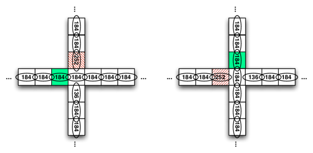
Each street is represented as an elementary cellular automaton (ECA), coupled at intersections. Each ECA contains a number of cells which can take values of zero (empty) or one (vehicle). The state of cells is updated synchronously taking into consideration their previous state and the previous state of their closest neighbors. Most cells simply allow a vehicle to advance if there is a free space ahead. This behavior is modeled with ECA rule 184 (See Table 1). At intersections, two other rules are used. Before a red light, vehicles do not advance, achieved with ECA rule 252. After a red light, crossing vehicles should not enter the street, achieved with ECA rule 136. The street with the green light uses only ECA rule 184. The intersection cells change neighbourhood to cells on the street with the green light, as shown in Figure 1.
| 000 | 0 | 0 | 0 |
| 001 | 0 | 0 | 0 |
| 010 | 0 | 1 | 0 |
| 011 | 1 | 1 | 1 |
| 100 | 1 | 1 | 0 |
| 101 | 1 | 1 | 0 |
| 110 | 0 | 1 | 0 |
| 111 | 1 | 1 | 1 |
This city traffic model is conservative, i.e. the density of vehicles (percentage of cells with a value of one) is constant in time. It is straightforward to extend it to an hexagonal grid, allowing for more complex intersections Gershenson and Rosenblueth (2012).
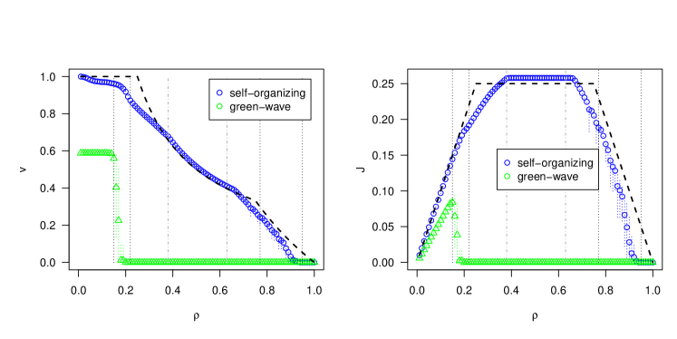
The average velocity is straightforward to calculate: it is given by the number of cells that changed from zero to one (movement occurred between time and ) divided by the total number of vehicles (cells with one). if no vehicle moves, while when all vehicles are moving.
Flow is defined as the velocity multiplied by the density , i.e. . when there is no flow: either there are no vehicles in the simulation () or all vehicles are stopped (). A maximum occurs when all intersections are being crossed by vehicles. In the studied scenarios, .
Theoretically, the optimum and for a given in a traffic light coordination problem should be the same as optimal and for isolated intersections, i.e. an upper limit. This implies that each intersection interacting with its neighbors is as efficient as one without interactions. This can be shown with “optimality curves” Gershenson and Rosenblueth (2012), visually and analytically comparing results of different methods with theoretical optima.
2.1.1 Non-orientable boundaries
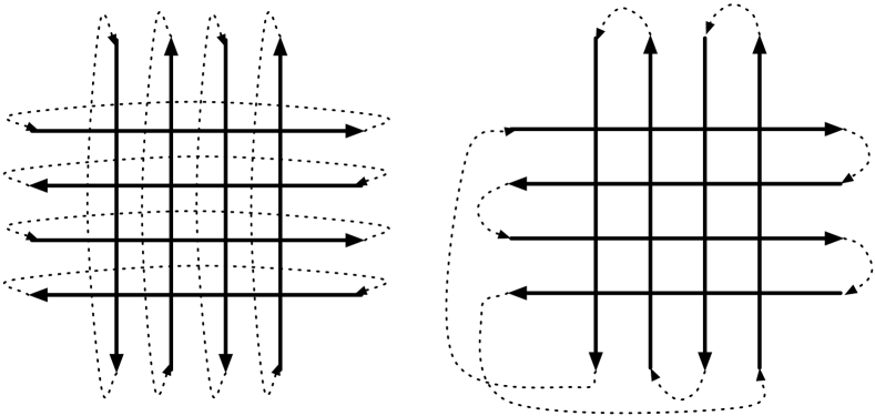
Our previous studies have assumed cyclic boundaries, as it is usual with ECA. However, this can lead to a quick stabilization of the system for certain densities, as vehicle trajectories become repetitive (assuming no turning probabilities, the model is deterministic).
Following a suggestion by Masahiro Kanai Kanai (2010), we changed the boundary conditions to be non-orientable (as in a Möbius strip or a Klein bottle), maintaining incoming vehicle distributions, constant density, and determinism but in practice destroying the correlations that were formed with cyclic boundaries.
Kanai Kanai (2010) studied an isolated intersection, also using ECA. Instead of having two cyclic ECA, he used a single self-intersecting ECA where vehicles exiting on the east enter from the north and vehicles exiting on the south enter from the west. Using a similar approach, changing the boundaries we transformed a ten by ten street scenario (twenty cyclic streets with one hundred intersections) to a single street self-intersecting a hundred times. An example of this change of boundaries is shown in Figure 2.
2.2 Traffic Light Coordination
The problem of coordinating traffic lights is EXPTIME-complete Papadimitriou and Tsitsiklis (1999). This implies that optimization for large traffic networks is unfeasible. Moreover, the precise traffic conditions change constantly (each cycle a different number of vehicles arrive at each intersection), so the problem is non-stationary. Even if we find an optimal solution, this becomes obsolete in seconds. Thus, an alternative to optimization becomes adaptation, being self-organization a useful method for building adaptive systems Gershenson (2007).
In this work we compare a traditional method which tries to optimize expected flows and a self-organizing method. These are described in detail in Gershenson and Rosenblueth (2012) and have been replicated in a parallel implementation, also available with source code at https://github.com/Zapotecatl/Traffic-Light
2.2.1 Green-wave method
Most cities try to synchronize their traffic lights using the so-called green-wave method Török and Kertész (1996). Traffic lights have the same period and the phase (offset) is adjusted so that green lights switch at the expected velocity of vehicles. In this way, once vehicles get a green light, they should not get any red light. This is better than having no coordination. However, due to mathematical constrains, at most two directions can have a green wave at the same time. Thus, vehicles driving in the opposite direction find anti-correlated phases and have high waiting times, leading to long queue formation already for medium densities. Moreover, if the vehicles do not go at the expected velocity (as it is the case when densities change), then vehicles will not be able to go at the speed of the green wave and will have to stop.
In Gershenson and Rosenblueth (2012) we studied the green wave method in the traffic model described in the previous subsection. We found only two dynamical phases: intermittent (some vehicles stop, some move) and gridlock (all vehicles are stopped).
2.2.2 Self-organizing method
We have proposed and refined a self-organizing method for traffic light coordination where each intersection follows simple local rules, reaching close to optimal global coordination Gershenson (2005); Cools et al. (2007); Gershenson and Rosenblueth (2012, 2012). The algorithm follows six simple rules, listed in Table 2. Rules with higher numbers override rules with lower numbers, e.g. rule 4 overrides rule 1.
![[Uncaptioned image]](/html/1402.0197/assets/x3.png) 1.
On every tick, add to a counter the number of vehicles
approaching or waiting at a red light within distance .
When this counter exceeds a threshold , switch the light.
Whenever the light switches, reset the counter to zero.
2.
Lights must remain green for a minimum time .
3.
If a few vehicles ( or fewer, but more than zero) are left to cross a green light at a short distance , do not switch the light.
4.
If no vehicle is approaching a green light within a distance , and at least one vehicle is approaching
the red light within a distance , then switch the light.
5.
If there is a vehicle stopped in the street a short distance
beyond a green traffic light, then switch the light.
6.
If there are vehicles stopped on both directions at a short distance
beyond the intersection, then switch both lights to red. Once one of the directions is free, restore the green light in that direction.
1.
On every tick, add to a counter the number of vehicles
approaching or waiting at a red light within distance .
When this counter exceeds a threshold , switch the light.
Whenever the light switches, reset the counter to zero.
2.
Lights must remain green for a minimum time .
3.
If a few vehicles ( or fewer, but more than zero) are left to cross a green light at a short distance , do not switch the light.
4.
If no vehicle is approaching a green light within a distance , and at least one vehicle is approaching
the red light within a distance , then switch the light.
5.
If there is a vehicle stopped in the street a short distance
beyond a green traffic light, then switch the light.
6.
If there are vehicles stopped on both directions at a short distance
beyond the intersection, then switch both lights to red. Once one of the directions is free, restore the green light in that direction.
Rule 1 gives preference to streets with higher demand (few vehicles wait more than several) and promotes the formation of platoons (few vehicles waiting may be joined by more to form larger groups, which reaching further intersections can trigger the green light before decreasing their speed). Rule 2 maintains a minimum green time to prevent fast switching of traffic lights in high densities. Rule 3 maintains platoons together, although allowing to split large platoons. Rule 4 is useful for low densities, allowing few vehicles to trigger a green light if there is no vehicle approaching the current green. Rules 5 and 6 are useful for high densities, switching lights to red if there are cars stopped downstream of the intersection, preventing its blockage. The pseduocode of the algorithm extended for multiple directions can be found in Gershenson and Rosenblueth (2012).
In Gershenson and Rosenblueth (2012) we found seven dynamical phases of the self-organizing method in our traffic model (with cyclic boundaries) as the density increases: free flow (no vehicle stops, ), quasi-free flow (almost no vehicle stops), intermittent underutilized (some vehicles stop, intersections do not reach maximum flow ), full capacity intermittent (some vehicles stop, i.e. all intersections have vehicles using them always), overutilized intermittent (some vehicles stop, intersections have to restrict both streams to prevent blockages using rule 6), quasi-gridlock (almost all vehicles are stopped, but “platoons” of spaces form and move in the direction opposite of streets), and gridlock (all vehicles are stopped, i.e. , as intersections get blocked from initial conditions). Their respective phase transitions occur approximately at values of and .
2.3 Measures
We recently proposed measures of emergence, self-organization, and complexity based on information theory in Gershenson and Fernández (2012) and refined them and based them on axioms in Fernández et al. (2014).
Shannon defined a measure of information Shannon (1948) equivalent to Boltzmann’s entropy depending of the probabilities for all symbols in a finite alphabet:
| (1) |
where is a positive constant. In this work, we consider the in eq. 4 to be of base two.
In its most general form, emergence can be understood as information produced by a process or system. Shannon’s information already measures this, so we defined
| (2) |
Minimum is given for regular, predictable strings (no new information produced), while maximum is given for irregular, pseudorandom strings (each symbol is new information). To bound to the interval we simply consider
| (3) |
where is the base used, i.e. the length of the alphabet (possible symbols which can occur in a string). For example, if , then equation 4 can be rewritten as:
| (4) |
since . In this work, we use base ten, i.e. . In our experience, a slight change of does not affect qualitatively the measures.
Self-organization can be seen as a reduction of entropy (Gershenson and Heylighen, 2003). Since is a type of entropy, we define
| (5) |
It might seem counterintuitive to define self-organization as the opposite of emergence, being both properties of complex systems. However, when taken to their limits, it can be seen that emergence is maximal in chaotic systems (, ) and self-organization is maximal in ordered systems (, ). It is when these are balanced that we can have complexity. Following López-Ruiz et al. Lopez-Ruiz et al. (1995), we define
| (6) |
where the 4 is included as a normalizing constant, bounding to .
Historically, Shannon defined information as entropy Shannon (1948) (equivalent to our ), while Wiener Wiener (1948) and von Bertanalffy von Bertalanffy (1968) defined information as its oposite, negentropy (equivalent to our ). Our measure of complexity reconciles these two opposing views, as a balance between order and chaos is maximal with a high . Dynamical systems such as cellular automata Langton (1990) and random Boolean networks Kauffman (1969, 1993); Gershenson (2004) have a maximal in the region their dynamics are considered most complex Gershenson and Fernández (2012). Since living systems also require a balance between adaptivity () and stability () Kauffman (1993); Balleza et al. (2008), can be used to characterize living systems, especially when comparing their with that of their environment Fernández et al. (2014). If we want artificial systems to exhibit the properties of living systems Bedau et al. (2009, 2013); Gershenson (2013a), then these should also have a high compared with that of their environment.
In this work, we measure the , , and of three different time series: of switching intervals, of vehicle intervals at an intersection, and of vehicle intervals at a street. These series measure the time between light switches of vehicles crossing a point. If these are completely regular, then and . If these were maximally chaotic, then and .
3 Results
Results in this section were obtained simulating a 10x10 street grid, each equidistant street representing 800m, i.e. 80m per block. A cell represents 5m (the distance between the front ends of stopped vehicles), and a time step one third of a second. Thus, represents 54km/h.
Simulations were performed for one hundred densities between 0.01 and 1, fifty runs per density value (5000 runs total with random initial conditions). Standard deviations are shown in figures, although these were minimal, except for some regions near phase transitions. Each run consisted of ten thousand time steps, of which only the second half were considered for generating the statistics.
All figures in the Results and Discussion sections show phase transitions of the self-organizing method for the cyclic boundary scenario with dotted lines for comparison.
3.1 Cyclic boundaries
As reported in Gershenson and Rosenblueth (2012), the performance—based on and —of the self-organizing method is superior to the green-wave method for all densities, as it can be seen in Figure 3. Here we include optimality curves Gershenson and Rosenblueth (2012), showing that the self-organizing method achieves or reaches a performance close to the theoretical optimum for a given density. The full capacity intermittent phase is optimal by definition, as well as the free flow phase. It can be seen that small improvements can still be made in the underutilized and overutilized phases, as well as the quasi-gridlock and gridlock phases.
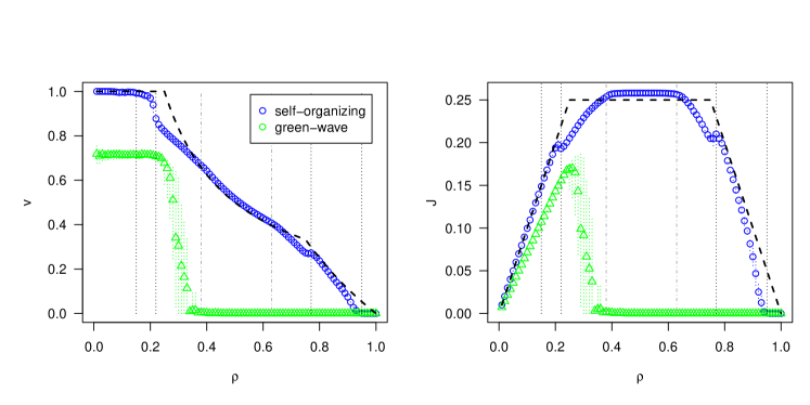
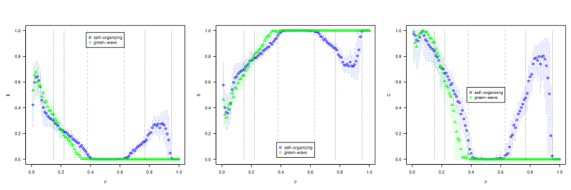
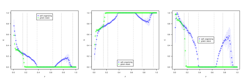
Figure 4 shows results of measures for switching intervals of intersections.
Since the green wave method has periodic cycles, for their switching and . Note that our measure does not distinguish whether the organization is internal (self-) or external, as it is the case for this method which depends on a central controller. Having extreme , it cannot adapt to changes in traffic flow.
The self-organizing method adapts constantly to changes in demand, as it can be seen from the measures variation for different densities. The switching is most irregular (greatest , lowest ) in the quasi-free flow and quasi-gridlock phases, while it achieves a regular switching (minimal and , maximal ) for the full-capacity intermittent phase, as there is always demand to be served from all directions. is high for all phases but full-capacity intermittent and gridlock, exhibiting similar measures as the green wave method for these two phases.
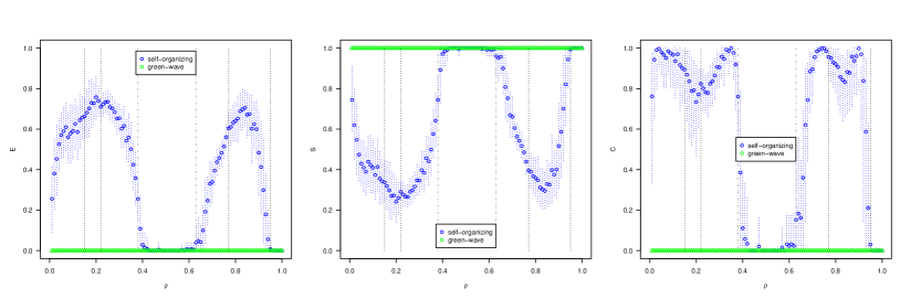
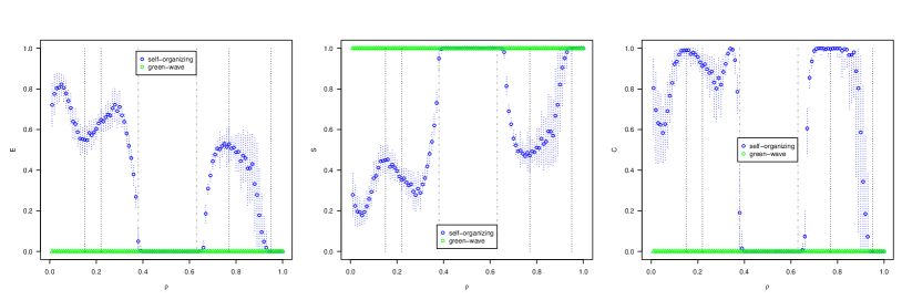
The measures of vehicles crossing at an intersection, as seen in Figure 5, are similar for the full capacity intermittent and gridlock phases, as there are either vehicles constantly crossing the intersection (there is a space between moving vehicles, so the intervals are constantly two time steps) or no vehicles moving (gridlock). and are high for low densities for both methods, and these become more regular ( increases) with until reaching a maximum in the full capacity intermittent phase for the self-organizing method and the gridlock phase in the green wave method. The self-organizing method increases again and until the quasi-gridlock phase, as vehicle crossings become less regular and “space platoons” are formed, only to decrease again towards the gridlock phase.
Vehicle intervals are measured at different street locations (not intersections) chosen randomly each run. These measures are similar to those from intersections described above, although they reach maximum only for the gridlock phase. There seems to be a minimum for the full capacity intermittent phase. Long platoons are formed, so most crossing intervals are two. However, between two platoons there are long spaces which imply a single long interval between the last vehicle of a platoon and the first one of the next platoon, giving minimum irregularity to the time series. Notice that is high for all phases except gridlock, for both methods, although differences can be easily identified between some phases of the self-organizing method. In other words, the dynamical phase can have a direct impact on , , and , which potentially could also be used to identify dynamical phases in more realistic traffic models, where transitions are not as crisp as in ours and thus could be difficult to identify.
3.2 Non-orientable boundaries
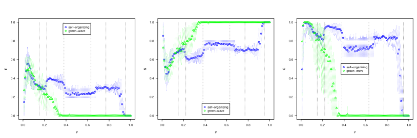
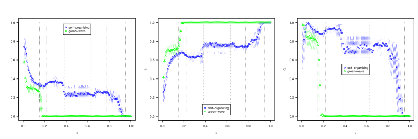
We performed similar simulations as the ones described in the previous subsection but with non-orientable boundaries. Results for and are shown in Figure 7, which indicates with dotted lines the phase transitions of the self-organizing method for the cyclic boundaries scenario for comparison.
Compared to the cyclic boundaries scenario, the green wave method has a lower for its intermittent phase and transitions into the gridlock phase at a lower density.
For the self-organizing method, there is no free-flow phase, as this depends on the correlations formed by the looping platoons which are destroyed with the non-orientable boundaries. The transition between the quasi-free flow and underutilized intermittent phases occurs at a lower density. The full capacity intermittent phase is expanded for higher densities, transitioning later into the quasi-gridlock phase. The transition between the quasi-gridlock and gridlock phases occurs at a slightly lower density.
In general, the self-organizing method maintains itself at or near the optimality curves, showing that its performance is not strongly dependent on the boundary conditions studied here.
As for the measures of , , and for switching intervals (Figure 8), vehicle intervals at intersections (Figure 9) and vehicle intervals at streets (Figure 10), there are no qualitative differences for the same dynamical phases between the cyclic and non-orientable boundary conditions.
4 Discussion
Changes in values of , , or can be used to detect phase transitions, as these can be radically different for different phases. This can also be achieved with other measures, such as Fisher information Prokopenko et al. (2011). However, it cannot be said whether a specific value of our measures is good or bad independently of density. There are traffic regimes where high regularity () of traffic lights is required to achieve optimal performance (full capacity intermittent phase), while there are other regimes, where a high adaptability () is necessary. This reflects the non-stationary nature of urban systems Gershenson (2013a), where no single solution is efficient for all situations, as these change constantly.
Not only traffic lights have to adapt their duration at the seconds scale to match the scale at which traffic demand changes. Traffic lights have also to adapt their regime at the scale at which density shifts from phase to phase. Extending Ashby’s law of requisite variety Ashby (1956), it can be said that there is a requisite complexity Gershenson (2012) that a controller must have in order to cope with the complexity of the system it attempts to control (Fernández et al., 2014, p. 47). This is similar to the “matching complexity” proposed by Tononi et al. (1996). Our self-organizing method seamlessly achieves this, giving insights on the requirements of other self-organizing systems which might be used for addressing non-stationary problems.
It might be possible to define measures which capture this requisite complexity and how it should match the complexity of the controlled/environment at different scales. One possibility can be with a measure of autopoiesis Fernández et al. (2014) which is defined as the ratio between the of a system (controller) and the of its environment (controlled). Further work is required in this direction, especially because in the self-organizing method traffic lights control vehicles, but vehicles also control traffic lights to a certain degree.
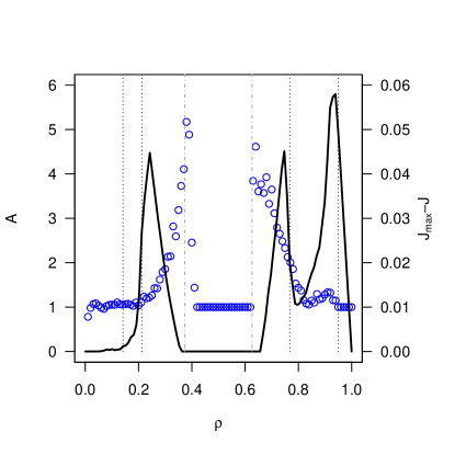
As an initial exploration, we compared the ratio between the switching intervals and vehicle intervals at intersections to obtain for the self-organizing method, shown in Figure 11. To avoid the indeterminacy of divisions by zero, only here we imposed a lower bound . The switching is almost always higher or equal than the vehicle at intersections (not always at streets), leading to . The highest values occur close to the phase transitions bordering the full capacity intermittent phase. These regions require a complex switching, and the self-organizing method manages to achieve this to regulate vehicle flow. Figure 11 also includes the difference between the optimality flow curve and the actual of the self-organizing method, to show where the method can still be improved. As mentioned previously, this is near the phase transitions between the quasi-free flow and underutilized intermittent phases and those around the quasi-gridlock phase. It could be speculated that to improve these regions should be further increased, either by augmenting the of the switching intervals or by decreasing the of the vehicle intervals. However, having already suggests that the lack of optimality for the specific densities close to the three mentioned phase transitions is due to inherent constrains in the problem. We conjecture that to reach around and it is necessary to have a homogeneous demand on all streets, so as to prevent “idling” of some intersections due to some streets having densities different from these values, which do vary in our simulations as initial conditions are random. A similar reasoning can be made for the region around the quasi-gridlock-gridlock phase transition: In order to allow vehicles on a single street with very high to have , initial conditions must be such that all of the intersecting streets must have a space available for the intersection and not others. This is highly unlikely for large grids with random initial conditions. Both constrains are dependent on the problem and beyond the traffic light coordination method.
From this study, we can generalize the use of our measures for guiding self-organization of other systems. We have seen that a desired value of depends on the regime which a system requires. If the system benefits from high regularity, then a high should be sought. If randomness or chaos are desired, then a high can be covetable. If adaptation is needed, then a high is advisable. In a control system, from our initial explorations of , a minimum value of the of the controller will depend on the of the controlled.
5 Future Work
The results presented in this paper are promising, but there are several points that should be further explored.
-
•
The relationship between dynamical phases and measures should be studied in greater detail.
-
•
The phase transitions in the non-orientable scenario can be further investigated, relating the performance measures such as and with the measures , , and .
-
•
We plan to perform similar studies with a more realistic traffic model Lárraga and Álvarez-Icaza (2010), adapted to city traffic.
-
•
Massive simulations with hundreds of streets and thousands of intersections are intended to better observe the dynamical phases and their transitions.
-
•
We have calculated the optimality curves for and . What would be the optimality curves for , and ? These cannot be simply extrapolated from the , and obtained for an optimal switching of an isolated intersection.
-
•
Can our measures be used to guide the self-organization of traffic lights even closer towards optimality?
-
•
Can our measures be used to guide the self-organization of other systems?
6 Conclusions
In this work we applied measures of emergence, self-organization, and complexity to an abstract city traffic model and compared two traffic light coordination methods. Varying boundary conditions yielded similar results. The measures reflect why the self-organizing method is much better than the green-wave method: for certain dynamical phases regular behavior is required, while for others adaptive, complex behavior is most efficient. The green-wave method by definition has only regular behavior, and thus is unable to adapt to constantly shifting demands. The self-organizing method has enough “requisite complexity” to cope with different behaviors required by changes in demand. Having an autopoiesis greater than one, it can be said that the self-organizing traffic lights have (computationally) the properties of a living system Gershenson (2012); Fernández et al. (2014), which also require to have a greater than their environment. Still, there are some regions which are not optimal. Whether these can be reached with a different method or they are computationally unfeasible (and our method then would be optimal in practice) still has to be explored.
This work shows an example of the usefulness of our proposed measures to guide the self-organization of systems, which are being applied in other areas as well Amoretti and Gershenson (2013); Fernández and Gershenson (2014); Febres et al. (2013). Since everything can be described as information Gershenson (2012), there is the potential of measuring , , and of every phenomena. Certainly, interpreting the meaning of a specific value at a particular scale is the real challenge.
Acknowledgements.
Acknowledgements C.G. was partially supported by SNI membership 47907 of CONACyT, Mexico. \conflictofinterestsConflicts of Interest The authors declare no conflicts of interest.References
- Cohen (2003) Cohen, J.E. Human Population: The Next Half Century. Science 2003, 302, 1172–1175.
- Butler (2010) Butler, D. Cities: The century of the city. Nature 2010, 467, 900–901.
- Roberts (2011) Roberts, L. 9 Billion? Science 2011, 333, 540–543.
- Glaeser (2011) Glaeser, E. Cities, Productivity, and Quality of Life. Science 2011, 333, 592–594.
- Bettencourt et al. (2007) Bettencourt, L.M.A.; Lobo, J.; Helbing, D.; Kühnert, C.; West, G.B. Growth, innovation, scaling, and the pace of life in cities. PNAS 2007, 104, 7301–7306.
- Bettencourt and West (2010) Bettencourt, L.; West, G. A unified theory of urban living. Nature 2010, 467, 912–913.
- Gyimesi et al. (2011) Gyimesi, K.; Vincent, C.; Lamba, N. Frustration Rising: IBM 2011 Commuter Pain Survey. 2011
- Gershenson (2013a) Gershenson, C. Living in Living Cities. Artificial Life 2013, 19, 401–420.
- Gershenson (2013b) Gershenson, C. The Implications of Interactions for Science and Philosophy. Foundations of Science 2013, 18, 781–790.
- Gershenson (2012) Gershenson, C. Self-organizing urban transportation systems. In Complexity Theories of Cities Have Come of Age: An Overview with Implications to Urban Planning and Design; Portugali, J.; Meyer, H.; Stolk, E.; Tan, E., Eds.; Springer: Berlin Heidelberg, 2012; pp. 269–279.
- Federal Highway Administration (2005) Federal Highway Administration. Traffic Control Systems Handbook; U.S. Department of Transportation, 2005.
- Henry et al. (1983) Henry, J.; Farges, J.; Tuffal, J. The PRODYN real time traffic algorithm. Proceedings of the Int. Fed. of Aut. Control (IFAC) Conf; , 1983.
- Mauro and Di Taranto (1990) Mauro, V.; Di Taranto, D. UTOPIA. Proceedings of the 6th IFAC / IFIP / IFORS Symposium on Control Computers and Communication in Transportation; , 1990.
- Robertson and Bretherton (1991) Robertson, D.; Bretherton, R. Optimizing networks of traffic signals in real time—the SCOOT method. Vehicular Technology, IEEE Transactions on 1991, 40, 11–15.
- Faieta and Huberman (1993) Faieta, B.; Huberman, B.A. Firefly: A Synchronization Strategy for Urban Traffic Control. Technical Report SSL-42, Xerox PARC, Palo Alto, CA, 1993.
- Gartner et al. (2001) Gartner, N.H.; Pooran, F.J.; Andrews, C.M. Implementation of the OPAC Adaptive Control Strategy in a Trafffic Signaling Network. IEEE Intelligent Transportation Systems Conference Proceedings, 2001, pp. 195–200.
- Diakaki et al. (2003) Diakaki, C.; Dinopoulou, V.; Aboudolas, K.; Papageorgiou, M.; Ben-Shabat, E.; Seider, E.; Leibov, A. Extensions and New Applications of the Traffic Signal Control Strategy TUC. Transportation Research Record 2003, 1856, 202–211.
- Fouladvand et al. (2004) Fouladvand, M.E.; Sadjadi, Z.; Shaebani, M.R. Optimized Traffic Flow at a Single Intersection: Traffic Responsive Signalization. J. Phys. A: Math. Gen. 2004, 37, 561–576.
- Mirchandani and Wang (2005) Mirchandani, P.; Wang, F.Y. RHODES to Intelligent Transportation Systems. IEEE Intelligent Systems 2005, 20, 10–15.
- Bazzan (2005) Bazzan, A.L.C. A Distributed Approach for Coordination of Traffic Signal Agents. Autonomous Agents and Multiagent Systems 2005, 10, 131–164.
- Helbing et al. (2005) Helbing, D.; Lämmer, S.; Lebacque, J.P. Self-organized control of irregular or perturbed network traffic. In Optimal Control and Dynamic Games; Deissenberg, C.; Hartl, R.F., Eds.; Springer: Dordrecht, 2005; pp. 239–274.
- Gershenson (2005) Gershenson, C. Self-Organizing Traffic Lights. Complex Systems 2005, 16, 29–53.
- Prokopenko (2009) Prokopenko, M. Guided self-organization. HFSP Journal 2009, 3, 287–289.
- Ay et al. (2012) Ay, N.; Der, R.; Prokopenko, M. Guided self-organization: perception–action loops of embodied systems. Theory in Biosciences 2012, 131, 125–127.
- Polani et al. (2013) Polani, D.; Prokopenko, M.; Yaeger, L.S. Information and Self-organization of Behavior. Advances in Complex Systems 2013, 16, 1303001.
- Prokopenko (2014) Prokopenko, M., Ed. Guided Self-Organization: Inception; Vol. 9, Emergence, Complexity and Computation, Springer: Berlin Heidelberg, 2014.
- Fernández et al. (2014) Fernández, N.; Maldonado, C.; Gershenson, C. Information Measures of Complexity, Emergence, Self-organization, Homeostasis, and Autopoiesis. In Guided Self-Organization: Inception; Prokopenko, M., Ed.; Springer: Berlin Heidelberg, 2014; Vol. 9, Emergence, Complexity and Computation, pp. 19–51.
- Wilensky (1999) Wilensky, U. NetLogo, 1999.
- Rosenblueth and Gershenson (2011) Rosenblueth, D.A.; Gershenson, C. A model of city traffic based on elementary cellular automata. Complex Systems 2011, 19, 305–322.
- Wuensche and Lesser (1992) Wuensche, A.; Lesser, M. The Global Dynamics of Cellular Automata; An Atlas of Basin of Attraction Fields of One-Dimensional Cellular Automata; Santa Fe Institute Studies in the Sciences of Complexity, Addison-Wesley: Reading, MA, 1992.
- Wolfram (2002) Wolfram, S. A New Kind of Science; Wolfram Media: Champaign, IL, USA, 2002.
- Gershenson and Rosenblueth (2012) Gershenson, C.; Rosenblueth, D.A. Self-organizing traffic lights at multiple-street intersections. Complexity 2012, 17, 23–39.
- Kanai (2010) Kanai, M. Calibration of the Particle Density in Cellular-Automaton Models for Traffic Flow. J. Phys. Soc. Jpn. 2010, 79, 075002.
- Papadimitriou and Tsitsiklis (1999) Papadimitriou, C.H.; Tsitsiklis, J.N. The Complexity of Optimal Queuing Network Control. Mathematics of Operations Research 1999, 24, 293–305.
- Gershenson (2007) Gershenson, C. Design and Control of Self-organizing Systems; CopIt Arxives: Mexico, 2007. http://tinyurl.com/DCSOS2007.
- Gershenson and Rosenblueth (2012) Gershenson, C.; Rosenblueth, D.A. Adaptive self-organization vs. static optimization: A qualitative comparison in traffic light coordination. Kybernetes 2012, 41, 386–403.
- Török and Kertész (1996) Török, J.; Kertész, J. The green wave model of two-dimensional traffic: Transitions in the flow properties and in the geometry of the traffic jam. Physica A 1996, 231, 515–533.
- Cools et al. (2007) Cools, S.B.; Gershenson, C.; D’Hooghe, B. Self-organizing traffic lights: A realistic simulation. In Self-Organization: Applied Multi-Agent Systems; Prokopenko, M., Ed.; Springer, 2007; chapter 3, pp. 41–49.
- Gershenson and Fernández (2012) Gershenson, C.; Fernández, N. Complexity and Information: Measuring Emergence, Self-organization, and Homeostasis at Multiple Scales. Complexity 2012, 18, 29–44.
- Shannon (1948) Shannon, C.E. A mathematical theory of communication. Bell System Technical Journal 1948, 27, 379–423 and 623–656.
- Gershenson and Heylighen (2003) Gershenson, C.; Heylighen, F. When Can We Call a System Self-Organizing? Advances in Artificial Life, 7th European Conference, ECAL 2003 LNAI 2801; Banzhaf, W.; Christaller, T.; Dittrich, P.; Kim, J.T.; Ziegler, J., Eds.; Springer: Berlin, 2003; pp. 606–614.
- Lopez-Ruiz et al. (1995) Lopez-Ruiz, R.; Mancini, H.L.; Calbet, X. A statistical measure of complexity. Physics Letters A 1995, 209, 321–326.
- Wiener (1948) Wiener, N. Cybernetics; or, Control and Communication in the Animal and the Machine.; Wiley and Sons: New York, 1948.
- von Bertalanffy (1968) von Bertalanffy, L. General System Theory: Foundations, Development, Applications; George Braziller: New York, 1968.
- Langton (1990) Langton, C. Computation at the Edge of Chaos: Phase Transitions and Emergent Computation. Physica D 1990, 42, 12–37.
- Kauffman (1969) Kauffman, S.A. Metabolic Stability and Epigenesis in Randomly Constructed Genetic Nets. Journal of Theoretical Biology 1969, 22, 437–467.
- Kauffman (1993) Kauffman, S.A. The Origins of Order; Oxford University Press: Oxford, UK, 1993.
- Gershenson (2004) Gershenson, C. Introduction to Random Boolean Networks. Workshop and Tutorial Proceedings, Ninth International Conference on the Simulation and Synthesis of Living Systems (ALife IX); Bedau, M.; Husbands, P.; Hutton, T.; Kumar, S.; Suzuki, H., Eds.; , 2004; pp. 160–173.
- Balleza et al. (2008) Balleza, E.; Alvarez-Buylla, E.R.; Chaos, A.; Kauffman, S.; Shmulevich, I.; Aldana, M. Critical Dynamics in Genetic Regulatory Networks: Examples from Four Kingdoms. PLoS ONE 2008, 3, e2456.
- Bedau et al. (2009) Bedau, M.A.; McCaskill, J.S.; Packard, N.H.; Rasmussen, S. Living Technology: Exploiting Life’s Principles in Technology. Artificial Life 2009, 16, 89–97.
- Bedau et al. (2013) Bedau, M.A.; McCaskill, J.S.; Packard, N.H.; Parke, E.C.; Rasmussen, S.R. Introduction to Recent Developments in Living Technology. Artificial Life 2013, 19, 291–298.
- Prokopenko et al. (2011) Prokopenko, M.; Lizier, J.T.; Obst, O.; Wang, X.R. Relating Fisher information to order parameters. Phys. Rev. E 2011, 84, 041116.
- Ashby (1956) Ashby, W.R. An Introduction to Cybernetics; Chapman & Hall: London, 1956.
- Gershenson (2012) Gershenson, C. The World as Evolving Information. In Unifying Themes in Complex Systems; Minai, A.; Braha, D.; Bar-Yam, Y., Eds.; Springer: Berlin Heidelberg, 2012; Vol. VII, pp. 100–115.
- Tononi et al. (1996) Tononi, G.; Sporns, O.; Edelman, G.M. A complexity measure for selective matching of signals by the brain. Proceedings of the National Academy of Sciences 1996, 93, 3422–3427.
- Lárraga and Álvarez-Icaza (2010) Lárraga, M.E.; Álvarez-Icaza, L. Cellular automaton model for traffic flow based on safe driving policies and human reactions. Physica A: Statistical Mechanics and its Applications 2010, 389, 5425–5438.
- Amoretti and Gershenson (2013) Amoretti, M.; Gershenson, C. Measuring the Complexity of Ultra-Large-Scale Evolutionary Systems. Submitted to Computer Networks, 2013
- Fernández and Gershenson (2014) Fernández, N.; Gershenson, C. Measuring Complexity in an Aquatic Ecosystem. In Advances in Computational Biology; Castillo, L.F.; Cristancho, M.; Isaza, G.; Pinzón, A.; Corchado Rodríguez, J.M., Eds.; Springer, 2014; Vol. 232, Advances in Intelligent Systems and Computing, pp. 83–89.
- Febres et al. (2013) Febres, G.; Jaffe, K.; Gershenson, C. Complexity measurement of natural and artificial languages. arxiv:1311.5427, 2013