Ring polymers with topological constraints

Abstract

In the first part of this work a summary is provided of some recent experiments and theoretical results which are relevant in the research of systems of polymer rings in nontrivial topological conformations. Next, some advances in modeling the behavior of single polymer knots are presented. The numerical simulations are performed with the help of the Wang-Landau Monte Carlo algorithm. To sample the polymer conformation a set of random transformations called pivot moves is used. The crucial problem of preserving the topology of the knots after each move is tackled with the help of two new techniques which are briefly explained. As an application, the results of an investigation of the effects of topology on the thermal properties of polymer knots is reported. In the end, original results are discussed concerning the use of parallelized codes to study polymers knots composed by a large number of segments within the Wang-Landau approach.

I Introduction

Polymer knots and links (see Ref. bookonknottheory for a definition of knots and links) have been actively studied since the discovery of interlocked polymer rings in DNA in 1961 by Frisch and Wasserman Frisch1961 . After then, linked DNA molecules were identified in HeLa cell in 1967 Hudson1967 . It has also been found that the probability that open circular DNA molecules link with supercoiled molecules is quite large Rybenkov1997 . Also in the production of artificial knots and catenanes there has been a fast progress. The first artificial polymer knot, a trefoil, has been synthetized in 1989 Dietrich-Buchecker1989 .

More recently, experiments have shown that bacterial DNA often occurs in the form of knots that are sometimes heavily linked together. For example, DNA molecules extracted from tailless mutants of phage P4 vir 1 del22 are highly knotted (95%) Arsuaga2005 . The mitochondrial DNA of Trypanosomes and related parasitic protozoa consists of networks of thousands of topologically interlocked DNA rings trypanosomes . This abundance of knot and links in cells occurs because the probability of knotting increases with the degree of confinement Micheletti2008 . Besides, a new mechanism of link formation in DNA has been detected Elbaz2012 .

Due to the progress of technology, the thermal and mechanical properties of polymer knots and links can now be studied experimentally. The mechanical properties of single polymer knots have been investigated for almost two decades with the help of optical tweezers and atomic force microscope tips. It has been discovered in this way that polymer strands containing knots are much more breakable under tension than straight filaments Arai1999 . Moreover, since a few years also the collective behavior of many polymer rings is accessible to experiments. The thermal properties of macromolecules forming knots and links may be analyzed using calorimetric techniques. For instance, in polymer fibers the presence of knots is revealed by irregularities in the thermogram Steinmann2013 . In artificial polymer materials, the existence of knots and links affects dramatically the viscoelastic properties of polymers. In Kapnistos2008 melts composed by entangled polymer rings of an unprecedented purity , i. e. containing only a small fraction of linear chains, have been obtained. It has been found by observing the power law stress relaxation of these melts that they have a much lower viscosity than those containing linear polymers, of about one order of magnitude less. What it is interesting, is that even a very low amount of linear open chains inside the melt is able to introduce relevant influence in the viscosity. For that reason, polymer knots and links in artificial materials can be used to fine tune the elastic behavior of the produced materials in industrial applications. The rheological properties of polymer melts of rings are actively studied in connection with their significant implications to our understanding of polymer dynamics. The mechanical properties of systems containing a few polymer rings entangled together under the tensions exerted by external forces play a relevant role also in the physics of DNA. More experimental results will come in the future thanks to more and more refined techniques of synthesis and separation of knotted polymers. Already now, the formation of polymer knots and the effects of the topology in the intramolecular interactions can be investigated experimentally, see e. g.Ohta2012 .

The experiments mentioned above allow the comparison between the observations and the predictions coming from theoretical models. For this reason, they have attracted the interest of the community of theoretical physicists. Theoretical models in turn provide a microscopic understanding of what is observed and can point out the directions of the future experimental research. Many approaches to what can well be called the problem of topological entanglement in polymer physics have been proposed. As a matter of fact, polymers are already complex systems by themselves. When they are further knotted and linked together, to this complexity one should also add the topological complexity. This makes the treatment of systems containing polymer knots and links very hard. The reward for solving this problem and achieving a better understanding of polymer melts and materials composed by topologically entangled polymer rings will be huge. The formation of links and knots can result in fact in important effects in the physical behavior of polymer materials, see Ref. Orlandini2007 for a review and further bibliography of this subject.

In describing the topological entanglement of polymer rings, it is possible to take advantage of the progresses made in the previous century in the classification of knots and links. In particular, one should mention in this respect the construction of powerful knot and link invariants like the polynomials of Alexander, HOMFLY and Conway or the invariants of Arf-Casson, Vassiliev–Kontsevich and several others. Following the seminal work of Witten Witten1989 it has been possible to derive expressions of knot and link invariants using a particular class of field theories that are denominated topological. To convince oneself that the abstract methods of knot theory really matter in practical applications, it is sufficient to mention the example of the DNA recombination procedure, during which the topology of DNA can be changed. The changes are performed by particular enzymes called topoisomerases. The action of these proteins cannot be observed directly, but it may be analyzed by the methods of knot theory, that have been indeed successfully applied in order to classify the effects of the topoisomerases Sumner1996 .

In polymer physics there has been always a nice interplay between experiments and theoretical approaches, both numerical and analytical. Perhaps the most important example of this is provided by the works of de Gennes and coworkers degennes ; cloizeaux , that have led to a satisfactory understanding of the behavior of polymers in a solution thanks to the use of renormalization group techniques. A similar interplay occurs also in the research on polymer rings subjected to topological entanglement. The formation of knots in polymer systems is probably the most well studied subject of the statistical mechanics of polymer knots. It can be tackled analytically by means of renormalization group methods. Nowadays there is a good agreement between analytical and numerical estimations of how the probability of formation of a knot of a given type scales with the length of the polymer rensburg . Numerical simulations on this subject have been started already in the mid-seventies with the pioneering works Vologodski1974 ; Vologodski1975 ; Frank-Kamenetskii1975 . Analytical methods are also able to predict the various scaling laws that characterize the asymptotic behavior of observables like the gyration radius. Moreover, links between pairs of polymers can be analytically modeled by using as the knot invariant that takes into account the topology the Gauss linking number. The model can be case in the form of a Ginzburg-Landau field theory which is similar to those appearing in the physics of critical systems. Its main characteristic is that the scalar fields creating and annihilating the monomers of the polymer trajectories are coupled with an Abelian BF model. The latter is a topological field theory and describes the ”reaction forces” due to the presence of the topological constraints. These constraints are necessary because, physically, two polymer trajectories cannot penetrate themselves unless the temperature is so high that the polymer melts down to single monomers or there are enzymes like the topoisomerases that allow the opening and the successive gluing back of the trajectories. It is intriguing the fact that BF models are invariant under parity and time reversal transformations and have been used for this reason as effective field theories in the description of high $T_{C}$ superconductors and topological insulators. With the help of the topological Ginzburg–Landau model mentioned above it has been possible to formulate concrete predictions on the behavior of linked polymers. First of all, it has been shown that the presence of the topological constraints on the polymer rings does not affect their critical behavior FFIL2 . Nevertheless, it affects the excluding volume interactions between the monomers by weakening them FFIL2 . The results of FFIL2 are valid in the approximation in which the monomer density is high and almost constant apart from small fluctuations. Let us note that attractive forces associated to topological constraints have effectively been observed in an experiment levene . Reviews on analytical methods can be found in KholodenkoVilgisPhysRep and in Kleinert’s book Kleinertbook .

Besides analytical calculations, very reliable numerical simulations allow to understand the behavior of polymer systems observed during experiments. A wealth of publications has been dedicated to the applications of polymer knots and links in biology and biochemistry, like for instance Micheletti2008 ; Weber2006 ; Sulkowska2008 ; Sulkowska2009 ; Galera-Prat2010 . More and more complex problems are solved. Examples are the recent advances in understanding the behavior of knotted proteins under stretching Sulkowska2008 ; Sulkowska2009 and the breakability of physical knots Pieranski2001 . Moreover, numerical simulations have shown that in localized knots as those studied in Arai1999 , the weakest points in the polymer strands are located at the two points in which the knot starts and ends Saitta1999 . Also numerical studies of the diffusion of polymer knots in gels have been able to reproduce the experimental results Weber2006 . Let us remember that these studies are relevant for the particular application of the phenomenon of gel electrophoresis, that allows to extract polymer knots of given types out of a mixture of polymer rings, e. g. DNA byproducts, having different topological configurations. The thermal properties of polymer knots in the stretched regime have been investigated very recently in paea ; yzff2013 . The latter works will be described in the next Sections. Very recently, some important advances in the statics and dynamics of polymer rings with or without entanglement have appeared in the literature kremer2011 ; sommer2013 . Numerical simulations are also important to investigate phenomena that are hardly accessible by experiments. For instance, despite the progress in understanding the viscoelastic properties of melts of polymer rings mentioned above, it is still difficult to isolate possible effects due to the presence in the melt of knots or links.

The rest of the paper is organized as follows. A short review on numerical approaches for treating the topological constraints of polymer knots is contained in Section II. In Section III, we present two fast techniques, namely the PAEA and TICI methods, which have been proposed in paea ; yzff2013 in order to preserve the topology of a polymer knot during the sampling procedure. The sampling is performed with the help of the Wang-Landau Monte Carlo algorithm, which is summarized in Section V. The PAEA and TICI methods allow the sampling of a huge set of knot conformations as it is required in the investigation of the thermal properties of unstretched polymer knots. Some of the results obtained with these methods are discussed in Section IV. The original part of this work can be found in Section V, where the conclusions are drawn and some further developments in the treatment of polymer knots with a large number of segments are presented.

II Numerical approaches to the problem of topological entanglement in polymer physics

The key to study the thermal and mechanical properties of polymer knots and links in both the analytical and numerical approaches consists in being able to preserve the initial topological configuration against the thermal fluctuations. Let us note that throughout this work, the word configuration refers to a particular topological state of a polymer knot. The word conformation will instead denote the particular shape in the space of the trajectory of a polymer knot in a given topological configuration. Topological constraints may be imposed on the possible knot conformations with the help of the so-called knot invariants (or link invariants in the case of links). Knot (link) invariants are mathematical quantities whose values, when computed for a particular knot (link), do not change under any continuous deformation of the knot (link), including stretching of its spatial trajectory, but not for example cutting and gluing. It should be kept in mind that there is no knot invariant that is able to distinguish every knot uniquely. The same statement is true for link invariants. The most common representations of knot and link invariants are polynomials or multiple contour integrals computed along the physical trajectories of the polymers. Let us recall at this point that these trajectories are usually approximated by continuous curves following Edwards’ approachedwards . This approximation is particularly suitable for analytical models. Numerically, the trajectories are discretized and become mechanical systems of beads connected together by segments. Some of the polynomial invariants, like the HOMFLY polynomials mentioned before, are very powerful in detecting different topological configurations. Recently, the A-polynomials and super A-polynomials have been isolated in the amplitudes of topological string theoriesApolynomials . These polynomials are able to distinguish knots and links from their mirror reflections, a feature that the HOMFLY polynomials do not possess. Let us note that, so far, it has been impossible to fix the topological constraints in analytical models of topologically entangled polymers based on the Edward approach with the help of polynomial invariants. The problem is that the coefficients of the polynomials characterizing this kind of invariants cannot be easily related to the physical trajectories of the polymers. Only the invariants expressed in the form of multiple contour integrals have been successfully applied up to now. This is the case of the Gauss linking number, which has been exploited to describe polymer systems with topological constraints imposed on the links between pairs of polymer rings FFIL ; FFIL2 ; FFIL3 . Links in which three or four rings are entangled may be described using Milnor type invariantsFFJMP2003 ; FFNOVA . Unfortunately, there are no such simple invariants like the Gauss linking number or the Milnor invariants that can be used to distinguish the topology of a knot. The situation is different in numerical simulations, in which mainly knot invariants in the polynomial form are considered, like the already mentioned Alexander polynomials or the HOMFLY polynomials, see for instance Vologodski1974 ; michalke . While the Alexander polynomials are not very powerful in detecting different knot topologies, their numerical evaluation is fast. The more refined HOMFLY polynomials require much more cpu-time to be computed. From this point on we will concentrate on numerical simulations of single polymer knots.

In order to treat the statistical mechanics of knotted polymers two main strategies can be devised. One strategy exploits self-avoiding random walks (SAW’s) probability1 ; probability2 ; probability3 on a lattice. A ring, possibly in a nontrivial topological configuration, is formed when the trajectory of the SAW intersects itself for the first time. With this procedure, after considering many SAW’s, it is possible to produce a statistically relevant amount of polymer knots. The probability $p_{N}({\cal K})$ of generating on a simple cubic lattice a rooted lattice polygon with $N$ segments and a given topological configuration ${\cal K}$ scales is very well known. It has been determined analytically and checked numerically by several authors, see for example work1 ; work2 . For large values of $N$, the expression of $p_{N}({\cal K})$ is given by:

$$p_{N}({\cal K})\sim N^{\alpha_{S}-2+N_{\cal K}}\mu^{N}$$ (1)

where the parameters $\mu$ and $\alpha_{S}$ are the called the growth constant and the entropic exponent respectively. $N_{\cal K}=1$ for prime knots. Of course, the type of the knot generated after the SAW intersects itself is a priori unknown. To determine it, knot invariants should be used.

The other strategy consists in starting from a seed configuration of the polymer system with a given topology. A statistically relevant set of different conformations of the system is then achieved applying on it random transformations. These transformations should satisfy a few requirements. First of all, they must be ergodic, so that all conformations can be accessible. For instance, the pivot moves proposed in Madras1990 have been proved to be ergodic in the case of rings if their topological state is not relevant Madras1990 ; yzff2013 . Basically, this means that, starting from a ring in an arbitrary conformation and in an arbitrary topological configuration, after applying to it a finite number of pivot moves it is always possible to arrive to a given seed conformation. However, the final conformation and the intermediate ones are not constrained to have the same topological configuration of the initial ring. In the case in which the pivot moves are not allowed to destroy the initial topology of the knot, which is relevant in the present context, there is no rigorous proof of their ergodicity, but only numerical evidencespaea ; yzff2013 .

To preserve the initial topological configuration of a knot after many random transformations, several different methods may be applied, which can be based on knot invariants or not. The fastest way to avoid unwanted changes of topology makes use of random transformations that, by construction, do not modify the topological configuration of the polymer knot. This is for instance the case of the BFACF elementary moves introduced in Refs. work3 ; work4 . In the literature work6 , the ergodicity of the BFACF algorithm has been rigorously proven. It has been shown in work7 that a Generalized Atmospheric Sampling articleonGAS implementation of the BFACF algorithm is able to sample the conformations of a trefoil knot consisting of lattice polygons containing up to thousands of edges. The techniques based on the BFACF moves are sampling the trajectories in the grand-canonical ensemble. This implies that the length of the knot may change, but the average length can be fine-tuned with an appropriate choice of the chemical potential in such a way that most frequently trajectories of a given length are obtained. There exist also topology preserving random transformations that work directly in the canonical ensemble, thus keeping fixed the length of the knot. An example is provided by the pull moves of Ref. pullmovesmainref , which have been applied in the case of polymer knots in swetnam . The main problem of the transformations that automatically keep fixed the topological configurations of the system is that they change only small portions of the knot trajectory. Especially for long polymers, this leads to slow equilibration times and also increases the time necessary for sampling the random conformations. A compromise is to allow somewhat larger transformations, but always not so large that a local analysis near the transformed element of the trajectory becomes insufficient to detect potential topology alterations. The first method of this kind, which is able to preserve the topology of knots on a simple cubic lattice by forbidding the bond-crossings resulting from pivot moves, has been proposed in 2012 paea . The details of this approach will be described in the next Section. A method that is similar in spirit, but is valid for off-lattice simulations, can also be found in the literature Narros . The idea of the algorithm of Narros is to decompose the collective pivot move, i. e. a move involving more than one monomer after a random transformation, into successive elementary moves. After each elementary move, one considers the triangle whose vertices are given by the new position of the moved monomer, it’s original position and the position of one of the adjacent monomers. The topology of the knot is preserved if there is no segment composing the knot that crosses the area spanned by such a triangle. The trial conformation is accepted after all elementary moves are performed and no bond-crossing takes place.

III The PAEA and TICI methods

In this Section we restrict ourselves to numerical investigations on the thermal properties of single polymer rings with different knot types. We choose the strategy of starting from a given seed conformation of the knot to be studied and then acting on it with random transformations in order to sample the set of all its possible conformations. The case of the thermal properties of polymer knots under stretching has been already studied a few years ago in swetnam . Here we treat unstretched polymers following Refs. paea ; yzff2013 . The problem of dealing with unstretched polymers is that they admit much more conformations than stretched ones. Indeed, for unstretched polymers containing a large number of segments, an enormous number of conformations needs to be generated to obtain a satisfactory statistics. If additionally the topological configuration of the polymer ring needs to be preserved, it is very important to develop powerful and time-saving methods to perform random transformations of its trajectory without violating the topological constraints. To this purpose, two new techniques have been developed in Refs. paea and yzff2013 . The first one, which is valid on a simple cubic lattice, is the so-called Pivot Algorithm and Excluded Area (PAEA) method paea . The polymer is realized as an ensemble of beads, called hereafter the monomers, connected together by segments of unitary length. The PAEA method uses as random transformations the pivot moves of Madras1990 . These random transformations are applied on a randomly chosen element of the knot trajectory starting from the $N_{0}-$th monomer and containing a number $K$ of contiguous segments. Of course $N_{0}$ varies randomly within the set of integers $1,\ldots,N$. The strategy of the PAEA method is based on the fact that the difference between the old and new conformations after each pivot move results in a closed loop $\Gamma$ (or, if $K$ is large enough, in a set of closed loops). In figure 1 we show as an example the loop formed after a pivot move on a trefoil knot $\cal T$.

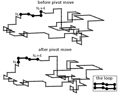
Figure 1: The upper picture shows a knot conformation ${\cal T}_{X}$ obtained after applying to a seed conformation with the trefoil topology a number $X=4$ of pivot transformations. Each pivot transformation changed an element of the knot containing a number $K=4$ of segments. The lower picture shows the new knot conformation ${\cal T}_{X+1}$ obtained after applying to ${\cal T}_{X}$ a trial pivot move. The small loop in the box appearing in the lower part of the picture in the right $\Delta{\cal T}_{X}$ is the difference between ${\cal T}_{X+1}$ and ${\cal T}_{X}$. The contour of $\Delta{\cal T}_{X}$ consists of the four segments from $N_{0}$ to $N_{0}+4$ belonging to ${\cal T}_{X}$ which have been chosen for the pivot transformation and of the four segments also from $N_{0}$ to $N_{0}+4$ of ${\cal T}_{X+1}$ obtained as a result of that transformation.

Around the loop $\Gamma$ we span an arbitrary surface having $\Gamma$ as its border. A trial pivot move is rejected if the trajectory of the old knot conformation crosses this surface or its border. It is easy to check that this is a necessary, but not sufficient, condition for the trial pivot transformation to change the topology of the knot. Irrespective of the fact that the topology has been really changed or not, the trial pivot move is rejected if the surface or its border are crossed at least once. This combination of pivot moves and the criterion of the excluded area, from which originates the name of the algorithm, provides an efficient and very fast way to preserve the topology that can be applied to any knot configuration, independently of its complexity. The time for evaluating if the trial pivot moves has destroyed the original topology or not scales as $\tau\sim N$. The main disadvantage of the PAEA method is that large pivot transformations are not easy to be implemented. To understand why, we remind that a pivot move involving $K$ segments will result in a closed loop (or loops) $\Gamma$ counting $2K$ segments. When $K=4$, one can easily classify all possible closed loops with $2K=8$ segments that may arise after such moves and construct appropriate surfaces having these loops as borders. The result are the eight loops displayed in Fig. 2.

Figure 2: In this figure all possible conformations of the small loop $\Gamma$ up to possible rotations and reflections have been listed for $K=4$. Arbitrary surfaces spanned by these loops have been drawn. The internal points have been denoted with squares.

Let us note that loops 2–8 have no internal points that can be intersected by the ”old” trajectory of the knot, which is the trajectory as it was before the action of the random transformation. Thus, only the intersections occurring at the borders of these loops must be checked. In the case of loop 1, instead, besides the border there is also one internal point that should be verified. If this point is intersected by the ”old” trajectory, then the topology of the knot obtained after the random transformation has certainly been changed. As $K$ increases, the number of closed loops becomes huge and the construction of the surfaces having these loops as borders becomes a difficult task. Up to now, the PAEA method has been realized in the case of $K=4$ and $K=5$. Our calculations based on the Wang-Landau Monte Carlo algorithmwanglandau , show that for polymers with $N=500$ segments, this is enough to ensure the necessary ergodicity and a reliable statistics. For longer polymers, the calculations may be finalized in a reasonable time only by means of techniques of parallel computing, which will be discussed later in Section V. An alternative, or at least complementary way, consists in developing methods that allow to preserve the topology for large random transformations, i. e. involving large elements of the knot. In fact, if the used random transformations affect only a small portion of the knot, the time for sampling increases as it was mentioned in the previous Section. In order to detect possible topology changes due to large random transformations, knot invariants in the polynomial form are certainly very suitable. As a matter of fact, apart from a few cases, they are quite powerful in distinguishing the topology and can be applied to whatever knot conformation, no matter how it has been changed after a random transformation. However, excluding the Alexander polynomials, the calculation of more sophisticated polynomials is time consuming. Thus, in yzff2013 it was explored the idea of applying knot invariants in the form of multiple contour integrals. The contours are the knot trajectory itself or elements of it. From that idea it originated the TICI method, where TICI stands for Topological Invariant in the form of Contour Integrals. Examples of invariants of that kind are abundant in the physical and mathematical literature, see for instance the Arf-Casson invariant GMMknotinvariant (equivalent to the Vassiliev invariant of degree 2otherauthormentioningVassilievknotinvariant ) or the Vassiliev-Kontsevich invariants kontsevich . The TICI method is based on the Vassiliev invariant of degree 2, denoted hereafter $\varrho(C)$.

Before yzff2013 , invariants in the integral representation have never been applied in numerical simulations of polymer physics. The only exception is the Gauss linking number, which has been exploited in numerical simulationsralf ; Kremer1 of systems of linked polymer pairs. The motivation of the little popularity of such invariants is probably the fact that their evaluation requires the computation of complicated multiple integrals. Let’s us remark that the time $\tau$ needed to evaluate a multiple integral with $l$ variables scales as $\tau\sim N^{l}$, where $N$ is the number of segments composing the polymer knot. However, it has been noticed in yzff2013 that the calculations can be sped up with the help of a suitable Monte Carlo integration algorithm and of parallelized codes. Besides, the Vassiliev knot invariant of degree 2 on which the TICI method is based, is one of the simplest knot invariant whose integral representation is known. The most time consuming integral to be computed is a quadruple one, so that $\tau\sim N^{4}$. Restricting ourselves to random transformations in which the number of involved segments $K$ is much smaller than the total number of segment $N$, this time can be reducedyzff2013 to $\tau\sim N^{3}$. This feature makes the use of $\varrho(C)$ competitive with respect to the Alexander polynomials. In fact, using the fastest approximation, the time required to evaluate the Alexander polynomial scales as $\tau\sim(M-1)^{3}$, see koniarismuthukumar . Here $M$ denotes the number of crossings which is necessary to draw the knot after projecting it on an arbitrary plane, seekoniarismuthukumar for more details. That approximation becomes not very precise when $M$ is large, a situation which is common in polymers confined in finite geometries. A further advantage of invariants expressed as multiple contour integrals with respect to polynomial invariants is their portability. They can be computed on or off-lattice without any modification. However, it should be mentioned the fact that their evaluation requires a smoothing procedure which becomes relatively complicated in the general case of polymers defined off-lattice ffyz2014 . Fig. 3 shows the effect of the smoothing procedure for an off lattice trefoil knot.

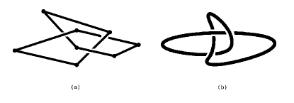
Figure 3: A trefoil knot with eight segments defined off lattice before and after the smoothing procedure.

Without the smoothing procedure, the computation of the knot invariant $\varrho(C)$ is affected by systematic errors due to the presence of the sharp corners at the joints between contiguous segments, but still it is possible to use it for the practical purpose of distinguishing the topology of different knot configurations. The comparison of the results of $\varrho(C)$ with and without the smoothing procedure for several knots is shown in Table 1ffyz2014 .

knot type	$\varrho_{a}(C)$	$\varrho_{sp}(C)$	$\varrho_{ns}(C)$	$n_{sc}$
$0_{1}$	$-\frac{1}{12}$	$-0.0839\pm 0.0332$	$+0.5526\pm 0.0569$	77
$3_{1}$	$+\frac{23}{12}$	$+1.9170\pm 0.0553$	$+2.4781\pm 0.0465$	68
$4_{1}$	$-\frac{25}{12}$	$-2.0847\pm 0.0533$	$-1.5214\pm 0.0845$	68
$5_{1}$	$+\frac{71}{12}$	$+5.9174\pm 0.0653$	$+6.4523\pm 0.0845$	65
$6_{1}$	$-\frac{49}{12}$	$-4.0856\pm 0.0723$	$-3.5717\pm 0.1007$	62
$7_{1}$	$+\frac{143}{12}$	$+11.9173\pm 0.0652$	$+12.4258\pm 0.1217$	62
$8_{1}$	$-\frac{73}{12}$	$-6.0822\pm 0.0529$	$-5.6380\pm 0.0774$	54
$9_{1}$	$+\frac{239}{12}$	$+19.9158\pm 0.0855$	$+20.4041\pm 0.1579$	59

Table 1: The values of the Vassiliev knot invariant of degree 2 for the knots with Alexander-Briggs notation $0_{1}$, $3_{1}$, $4_{1}$, $5_{1}$, $6_{1}$, $7_{1}$, $8_{1}$ and $9_{1}$. $\varrho_{a}(C)$ denotes the analytical value of the knot invariant. $\varrho_{sp}(C)$ is the results of the knot invariant with the smoothing procedure described in ffyz2014 . $\varrho_{ns}(C)$ is instead the value of the knot invariant derived without the smoothing procedure. The data of $\varrho_{sp}(C)$ and $\varrho_{ns}(C)$ have been computed using the same number of samples, which varies depending on the kind of knot. $n_{sc}$ is the number of sharp corners contained in the knot before the smoothing procedure.

In writing Table 1 we took advantage of the fact that $\varrho(C)$ is related to the second coefficient $a_{2}(C)$ of the Conway polynomials GMMknotinvariant by the following equation:

$$a_{2}(C)=\frac{1}{2}\left[\varrho(C)+\frac{1}{12}\right]$$ (2)

Since the coefficients $a_{2}(C)$ can be computed analytically for any type of knots, the analytical values of $\varrho(C)$ are also known for any given knot configuration. Compared with the PAEA method, the use of $\varrho(C)$ reduces the number of samples necessary for the calculations of the averages of the observables with the Wang-Landau Monte Carlo algorithmyzff2013 . This reduction is probably due to the fact that with $\varrho(C)$ large pivot transformations can be exploited, which are able to change relevant portions of the knot. In this way, the exploration of the whole set of available conformations becomes faster. Despite the decreasing of the number of samples, the computations still last in general longer than those performed with the PAEA method, because the expression of $\varrho(C)$ contains quadruple integrals that should be evaluated numerically and this is time consuming. Several tricks to reduce this time have been proposed in Refs. yzff2013 ; ffyz2014 . The most effective is the possibility of reducing on a simple cubic lattice the number of segments $N$ by a factor three.

IV Thermal properties of polymer knots

As an application of the fast methods presented in the previous Section, the thermal properties of several knots are computed using the Wang-Landau algorithm wanglandau . This has been done in Ref. paea with the help of the PAEA method. The implementation of the TICI method to the study of the statistical mechanics of polymer knots can be found in Ref. yzff2013 . The computational details of the TICI method may be found in Ref. ffyz2014 . Here a brief account of these results will be provided. Polymers are defined on a simple cubic lattice, with the monomers located at the sites of the lattice. Very short-range forces between the monomers are assumed. The related potential is defined as follows:

$$V_{IJ}=\left\{\begin{array}[]{rl}+\infty&\mbox{if $I=J$}\\ \varepsilon&\mbox{if $d=|\vec{R}_{I}-\vec{R}_{J}|=1$ and $I\neq J\pm 1$}\\ 0&\mbox{otherwise}\end{array}\right.$$ (3)

where $\varepsilon$ is the interaction energy between pairs of non-bonded monomers. The condition $\varepsilon<0$ refers to the case of attractive forces, while $\varepsilon>0$ characterizes the repulsive case. Moreover, $\vec{R}_{I}$ denotes the position vector of the $I$-th segment.

In Refs. paea and yzff2013 the specific energy, the specific heat capacity and the gyration radius of several types of polymer knots have been computed. In Fig. 4 we show the results of the computation of the specific heat capacity obtained with the TICI method for a trefoil knot in both attractive (left panel) and repulsive cases (right panel) yzff2013 . The rings contain a relatively small number of segments $N\leq 90$, because the purpose of yzff2013 was to study the influences of topology on the thermal behavior of polymer knots. These influences are much more marked if the polymers are short. This point will be discussed later in further details.

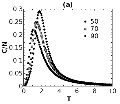
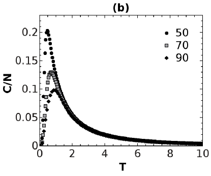
Figure 4: The specific heat capacity (in units of $\varepsilon$) of the trefoil as a function of the normalized temperature $\mathbf{T}=\frac{T}{\varepsilon}$ in both (a) the attractive and (b) the repulsive cases. The number of segments can take the values $N=50$ (circles), $N=70$ (rectangles) and $N=90$ (diamonds).

We discuss here mainly the case in which the potential is attractive, corresponding to Fig. 4 (a). The peak in the specific heat capacity is interpreted as a pseudo phase transition from a frozen crystallite state to an expanded state. This is a pseudo phase transition because we are working with a finite size system, far from the thermodynamic limit, as discussed in Refs. wuest ; janke . In janke it has been stressed that such pseudo phase transitions will become more and more important, because they will soon be observable in real systems thanks to the advances in the construction of high resolution equipment. The behavior of the specific heat capacity has been related with the presence of a pseudo phase transition by observing that the peak of the heat capacity at the pseudo phase transition grows more or less linearly with the increasing of the number of segments $N$ as it is expected. Indeed, the peak of the specific heat capacity remains at an almost constant height independently of the value of $N$. This fact is evident also from Fig. 5 (a), where polymer knots with $N=100,200$ and $300$ are considered.

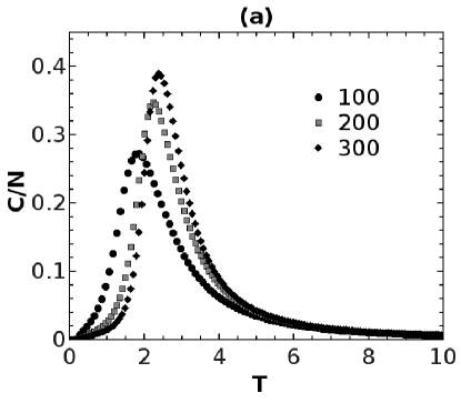
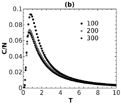
Figure 5: The specific heat capacity (in units of $\varepsilon$) of the trefoil as function of the normalized temperature $\mathbf{T}=\frac{T}{\varepsilon}$ in both (a) the attractive and (b) the repulsive cases. The number of polymer segments can take the values $N=100$ (circles), $200$ (rectangles) and $300$ (diamonds).

Another reason hinting that a pseudo phase transition is undergoing is coming from the plot of the gyration radius, which during the transition increases considerably (more than 50%), see Ref. yzff2013 . The nature of the initial and final states has been decided by examining directly the knot conformations. Before the transition, at low temperatures, the knot exhibits a partially ordered structure similar to that of a crystal, with defects which are probably related to the topological constraints and the knotting. Similar pseudo phase transitions from a frozen crystallite state to an expanded state have also been detected in the case of a single polymer chain discussed in binder . We see only one peak, because we are dealing with very short-range interactions, in agreement with Ref.binder , in which it was found that, if the range of the interactions is very short, then the open chain admits just two possible states, namely the crystallite and the expanded coil ones. Let us notice that pseudo phase transitions under stretching have been already observed in knots, see swetnam .

The presence of sharp peaks in the heat capacities in the repulsive case, see Figs. 4 (b) and 5 (b), has not a straightforward interpretation like those occurring when the interactions are attractive. The data concerning the gyration radius, in fact, show only a modest increase of this quantity in the range of temperatures in which the supposed pseudo phase transition is undergoing. Moreover, the temperature at which the peak occurs is rather low and, actually, the height of the peak seems to decrease with increasing numbers of segment $N$. As argued in yzff2013 , the peak in the heat capacity is almost probably due to a lattice artifact, related to the fact that, when the temperature is very low, the first energy state $E_{1}=\varepsilon$ cannot be reached, because $kT<E_{1}$. So the system stays in the ground level $E_{0}=0$ and only when $kT$ becomes big enough, it jumps to the next states $E_{1},E_{2},\ldots$. Let us remark that the behavior of the thermal properties in the repulsive case is in agreement with the previous results of Ref. work8 , where it has been studied the dependence on the ion concentration of the specific energy and the gyration radius of a mixture of knotted and unknotted polymer rings in a salty solution. The comparison is made difficult by the fact that the systems and the interactions discussed here and in work8 are different. However, in the repulsive case discussed here, we expect that the very short-range interactions become irrelevant when the temperature is high. Analogously, when the ion strength is low, the polymer knot is immersed in a good solvent, thus experiencing repulsive forces, which are fading away with the increasing of the ion strength. As a consequence, we can qualitatively compare the behavior of a polymer knot for increasing temperature and the behavior exhibited by the knot for growing ion strength.

The topological effects on the thermal properties of knotted polymer rings have been discussed in the paper yzff2013 by comparing knots of different types but of the same length. It was shown inyzff2013 that the topology of knots plays an important role when the size of the polymer is small. Moreover, topology related effects disappear with increasing polymer lengths. This fact can also be confirmed by the calculation of the gyration radii. Following the work of deguchi3 , for instance, the values of the normalized gyration radius $\frac{\langle R_{\cal K}^{2}\rangle}{\langle R^{2}\rangle}$ can be plotted as in Fig. 6 for different polymer lengths up to $N=400$. Here $\langle R^{2}\rangle=\frac{1}{3}\sum_{\cal K}\langle R_{\cal K}^{2}\rangle$ denotes the average of the gyration radius of a closed polymer trajectory of fixed length irrespective of its topological configuration $\cal K$.

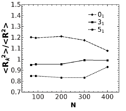
Figure 6: Plot of the normalized gyration radius $\frac{\langle R^{2}_{\cal K}\rangle}{\langle R^{2}\rangle}$ for knots of different topology ${\cal K}=0_{1},3_{1},5_{1}$ and of different number of segments $N=70,90,200,300,400$. For increasing values of $N$, the normalized gyration radii of different knots appear to converge to the same value $1$.

The sum over ${\cal K}$ has been limited to the knot types ${\cal K}=0_{1},3_{1},5_{1}$, which is the reason of the factor $\frac{1}{3}$ in the expression of $\langle R^{2}\rangle$. Clearly, in the case in which there are no effects on the gyration radius related to the fact that the three knots $0_{1},3_{1},5_{1}$ are topologically different, we would have that $\frac{\langle R^{2}_{\cal K}\rangle}{\langle R^{2}\rangle}=1$ for ${\cal K}=0_{1},3_{1},5_{1}$. The normalized gyration radius $\langle R_{\cal K}^{2}\rangle$ of each knot ${\cal K}$ with ${\cal K}=0_{1},3_{1},5_{1}$ has been computed using a set of $50\times 10^{6}$ conformations. Fig. 6 suggests that the values of the normalized gyration radius converge in the limit $N\longrightarrow\infty$, a fact that implies that the dependence on the knot type is disappearing with increasing number of segments $N$.

V Further developments and conclusions

To preserve the topology of polymer knots during the sampling procedure needed in Monte Carlo simulations, two algorithms, namely the PAEA and the TICI methods, have been presented in Section. III. The performance of the PAEA method is independent of the complexity of the knot and the time needed for accepting or rejecting a given conformation after a random transformation grows linearly with the number of segments composing the knot. This makes the PAEA method very fast. Its disadvantage is the difficulty of its implementation for random transformations involving more than $K=5$ segments. On the other side, the TICI method is significantly slower, because the time for computing the Vassiliev invariant of degree 2 scales with $N$ as $\tau\sim N^{4}$. After several improvements, with the TICI method it is currently possible to treat in a reasonable time the statistical properties of polymer knots up to 400 segments. The advantage of this method is that large portions of the knot may be changed randomly with a single transformation. This speeds up the sampling of different conformations. Moreover, the TICI method works both on and off-lattice without modifications and is easily generalizable to the case of links composed by three linked rings. As a matter of fact, the triple Milnor invariant describing the topological configurations of links among three rings consists in a linear combination of terms that are very similar to the Vassiliev invariant of degree 2 used in the TICI method.

Despite these progresses, the treatment of very long polymers or of many polymers within the Wang-Landau algorithm becomes difficult when $N\sim 1000$. For this reason, one should rely on parallelized codes. The parallelization of the Wang-Landau algorithm has been discussed in Ref. yanlan and, more recently, also in tholan The reader is addressed to these works for additional bibliography on this subject. Here we would like to present two ways to implement the parallelization of the Wang-Landau algorithm which are suitable for polymer simulations. Before doing that, however, a few words about the Wang-Landau terminology is in order. The details are reported in the original article wanglandau . The goal of the Wang-Landau procedure is to compute the so-called density of states $\phi_{m}$ for the energy values $E_{m}$ in a given energy domain $D$. In principle $D$ should cover the whole energy spectrum. We assume for simplicity that the various energy levels $E_{m}$ are labeled by positive integer numbers, so that $m=1,2,\ldots$. $\phi_{m}$ represents the number of conformations having energy $E_{m}$. Its expression is:

$$\phi_{m}=\sum_{X}\delta(H(X)-E_{m})$$ (4)

where $X$ is an arbitrary conformation with fixed topological configuration and $H(X)$ is the Hamiltonian. $\phi_{m}$ plays the same role of the number of states in the microcanonical ensemble. Its relation with the partition function $Z$ in the canonical ensemble is:

$$Z=\sum_{m}e^{-\beta E_{m}}\phi_{m}$$ (5)

with $\beta$ being the Boltzmann factor. The Wang-Landau algorithm computes the density of states perturbatively in a finite number of steps. At the $\nu-$th step, the precision is determined by the so-called modification factor $f_{\nu}$. Each $f_{\nu}$ is defined by the relation: $f_{\nu}=f_{0}^{\frac{1}{2^{\nu}}}$, where $f_{0}>1$ is the value of the modification factor at the zeroth approximation. Usually, $f_{0}$ is chosen to be equal to $e$. At the beginning, the density of states has the initial value $\phi_{m}=1$ for all energy levels. Successively, $\phi_{m}$ is updated with the following procedure. At each approximation order $\nu$, different conformations of the knot are randomly generated. A conformation $X_{m^{\prime}}$ of energy $E_{m^{\prime}}$ obtained after a random transformation of a previous conformation $X_{m}$ of energy $E_{m}$, is accepted unconditionally if the transition probability:

$$p(X_{m}\longrightarrow X_{m^{\prime}})=\min\left\{1,\frac{\phi_{m}}{\phi_{m^{\prime}}}\right\}$$ (6)

is equal to one. Otherwise, a random number $\eta$ such that $0<\eta<1$ is generated and the new conformation $X_{m^{\prime}}$ is accepted if $p(X_{m}\longrightarrow X_{m^{\prime}})>\eta$. In all other cases $X_{m^{\prime}}$ is rejected. If $X_{m^{\prime}}$ has been accepted, then the density of states and the energy histogram $h_{\nu}(E_{m})$ are updated as follows: $\phi_{m^{\prime}}\longrightarrow f_{\nu}\phi_{m^{\prime}}$ and $h_{\nu}(E_{m^{\prime}})\longrightarrow h_{\nu}(E_{m^{\prime}})+1$. The next approximation level $\nu+1$ starts when the histogram $h_{\nu}(E_{m})$ of the conformations at the $\nu-$th order becomes flat within a precision of $\pm 20\%$.

A possible parallelization strategy for performing the sampling necessary in the Wang-Landau algorithm consists in splitting the task into a number $J$ of threads $t_{1},\ldots,t_{J}$ . All threads explore simultaneously conformations in the whole energy spectrum. The threads work in cycles. At the beginning of a cycle, the global density of states $\phi_{m}^{\prime}$ is the same for all threads. During the cycle, each thread samples a set of $\ell$ conformations and updates independently of the others the density of states. The value of $\ell$ depends on the number of threads. At the end of the cycle, every thread $t_{s}$, with $1\leq s\leq J$, has updated the density of states $\phi_{m}^{\prime}$ by a factor $\Delta\phi_{m,s}^{\prime}$, The new density of states according to the $s-$th thread will be thus given by: $\phi_{m,s}^{\prime}=\phi_{m}^{\prime}\Delta\phi_{m,s}^{\prime}$. The new global density of states $\phi_{m}^{\prime\prime}$ is obtained by averaging over all the results coming from the $J$ threads:

$$\phi_{m}^{\prime\prime}=\sqrt[J]{\prod_{s=1}^{J}\phi_{m,s}^{\prime}}$$ (7)

At this point, a new cycle starts and the density of states $\phi_{m}^{\prime\prime}$ is updated separately a number $J$ of times by the threads. After sampling an additional set of $\ell$ conformations, the next corrections $\Delta\phi_{m,s}^{\prime\prime}$ to $\phi_{m}^{\prime\prime}$ are computed and the global density of states $\phi_{m}^{\prime\prime\prime}$ may be obtained using the geometrical averaging of Eq. (7). The procedure continues until the energy histogram becomes flat, after which the next approximation level is started. With this method, the threads are allowed to sample the set of all possible conformations independently, but only for the limited number of samples $\ell$ generated during a cycle. When the cycle ends, the information collected by the different threads gets ”exchanged” by the averaging process of Eq. (7). This procedure avoids the situation in which the threads update the density of states in a totally independent way. Large scale simulations show that in this case there can be difficulties in estimating the correct density of states $\phi_{m}$, see Ref. tholan on that point.

Using the parallelization techniques described above, together with the PAEA method to detect topology changes of the knot after a random transformation, it is possible to study polymer knots subjected to very short interactions like those of Eq. (3) in a reasonable time of weeks and with a satisfactory level of approximation if the number of segments in the knot is of the order $N\sim 1000$ or less. For a polymer with $N=1000$, the approximation level $\nu=15$ is reached within the time of one month using $J=12$ threads. For greater values of $N$, the number of threads should be increased. Thus, to prevent possible problems related to the simultaneous running of a huge amount of threads, following tholan it is reasonable to adopt a strategy in which the energy domain is split into many different regions $D_{1},\ldots,D_{L}$. In each domain $D_{j}$, $j=1,\ldots,L$, the energies $E_{m}$ are limited to the interval $[E^{i}_{min},E^{i}_{max}]$. The energy values in these regions partly overlap, i. e. the set $D^{j}\cup D^{j+1}=[E^{j+1}_{min},E^{j}_{max}]$ is not empty. The goal is to evaluate separately the partial densities of states $\phi^{1}_{m},\phi_{m}^{2},\ldots,\phi^{L}_{m}$ in the regions $D^{1},D^{2},\ldots,D^{L}$ respectively. As we will see, the global density of states $\phi_{m}$ can be reconstructed if all the partial densities of states are known. Of course, as mentioned in yanlan and tholan , with the splitting of the total energy domain in subdomains some statistically relevant set of conformations may be ignored. For polymers, this is particularly true in the case of very compact conformations. Indeed, if during the sampling a class of very compact conformations is obtained, sometimes it could be necessary to unpack the knot to some extent and then pack it again in another way in order to reach a class of even more compact conformations. When the knot gets unpacked, the distances between the monomers increase in the average, a fact that is connected with a change of the total potential energy of the system. If the sampling is restricted to a particular energy region, it may well be happen that the energy value that should be attained to allow the unpacking of the knot lies outside that region. This simple example shows how all conformations that may be obtained only by unpacking and repacking the knot starting from a given seed conformation could become not accessible after the splitting of the energy domain in many regions. To circumvent this problem, we choose a somewhat different approach from that of tholan , that will be called here the splitting method. We assume now that we are just interested in computing the density of states $\phi^{i}_{m}$ in the particular interval of energies $D_{i}=[E^{i}_{min},E^{i}_{max}]$ for some value of $i$, with $1\leq i\leq L$. The basic idea is that to speed up the calculations, avoiding to have to consider the whole energy spectrum, it is not necessary to restrict the sampling only to the region $D_{i}$. It is sufficient to limit the time spent by the code in analyzing the other regions. To this purpose, the exploration of the regions $D_{j}$ with $j\neq i$ can be penalized by increasing appropriately the modification factor $f_{\nu}$ outside $D_{i}$. Let $f_{i,\nu}^{j}$ be the modification factor that will be used in the interval $[E^{j}_{min},E^{j}_{max}]$, $j=1,\ldots,L$, to evaluate the density of states $\phi_{m}^{i}$. We define the $f_{i,\nu}^{j}$’s as follows:

$$f_{i,\nu}^{j}=\left\{\begin{array}[]{ccc}f_{0}^{\frac{1}{2^{\nu}}}|E^{j}_{max}-E^{i}_{min}|^{\alpha_{j}}&\mbox{for}&j<i\\ f_{0}^{\frac{1}{2^{\nu}}}|E^{j}_{min}-E^{i}_{max}|^{\alpha_{j}}&\mbox{for}&j>i\\ f_{0}^{\frac{1}{2^{\nu}}}&\mbox{for}&j=i\end{array}\right.$$ (8)

where the $\alpha_{j}$’s are suitably chosen constants. In other words, in the energy region of interest $D_{i}$, $f_{i,\nu}^{i}$ is the usual modification factor of the Wang-Landau algorithm at the approximation level $\nu$. However, the $f_{i,\nu}^{j}$’s have been increased by factors that are proportional to some power $\alpha_{j}$ of the minimal distance on the energy axis between the energy values in $D^{i}$ and $D^{j}$. A good choice of $\alpha_{j}$ is for instance $\alpha_{j}=1$ for $j\neq i$. With the splitting method just outlined, the sampling is performed in every energy region, but most of the time is spent to sample the conformations in the selected region $D_{i}$. When the energy histogram becomes flat in the interval $[E^{i}_{min},E^{i}_{max}]$, the next level of approximation in computing the density of states $\phi^{i}_{m}$ is started. The simulations show that also configurations whose energy is not in the chosen region $D_{i}$ are visited several times, but of course much less than the conformations with energy in the range $[E^{i}_{min},E^{i}_{max}]$, because the transition probability (6) to all conformations outside $D_{i}$ is suppressed by the choice of modification factors in Eq.(8). Let’s now consider the case of regions in which the monomer density is high. Exactly these conformations are difficult to be sampled as discussed earlier. Assuming that the interactions are attractive, they correspond to regions in which the energy is very low. If, starting from a given seed conformation, the system is trapped during the sampling in a class of conformations of very low energy which is not statistically relevant, with the method explained before the knot is still able to slowly unpack itself under the effect of random transformations reaching domains of higher energy. After some time is passed, a longer stay in these domains becomes very unlikely due to the transition probability (6) and the choice of modification factors (8). As a consequence, the conformations drift back toward the region of very low energy and the knot gets packed again. After a conformation $X_{low}$ with energy belonging to the selected region $D_{i}$ is reached, the system remains in that region for a long time. The conformation $X_{low}$ becomes the new seed, starting from which a large number of conformations in the selected energy region is sampled. Of course, we expect that, especially for long polymers, after the knot is unpacked and repacked in this way several times, it attains seed conformations $X_{low}^{(1)},X_{low}^{(2)},X_{low}^{(3)},\ldots$ that belong to a class of conformations with energies in $D_{i}$ whose number is overwhelmingly larger than that of more rare conformations in the same energy range.

In Fig. 7 we compare

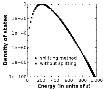
Figure 7: Comparison of the densities of states for a knot $5_{1}$ with number of segments $N=1000$ computed with the splitting method (dots) and without it (squares).

the densities of states for a knot $5_{1}$ with $N=1000$ segments computed with or without the splitting method. The total density of states $\phi_{m}$ has been obtained from the partial densities of states $\phi_{i,m}$ derived from the splitting method as follows. First, it is checked if at the intersection between two contiguous energy domains $D_{i}\cap D_{i+1}$, the partial density of states in $D_{i+1}$ coincides with that of $D_{i}$. Let $(\phi_{i,m},\phi_{i+1,m})$ and $(\phi_{i,m^{\prime}},\phi_{i+1,m^{\prime}})$ be two pairs of densities of states corresponding to the energies $E_{m}$ and $E_{m^{\prime}}$ respectively. $\phi_{i,m}$ and $\phi_{i+1,m}$, as well as $\phi_{i,m^{\prime}}$ and $\phi_{i+1,m^{\prime}}$, are the partial density of states resulting from the sampling in the regions $D_{i}$ and $D_{i+1}$ respectively. If both energy values $E_{m}$ and $E_{m^{\prime}}$ belong to the intersection domain $D_{i}\cap D_{i+1}$, then we have found from our simulations that the ratio $\frac{\phi_{i,m}}{\phi_{i+1,m}}$ is almost equal to the ratio $\frac{\phi_{i,m^{\prime}}}{\phi_{i+1,m^{\prime}}}$ within the required level of approximation $\nu$. This means that two partial densities of states calculated in contiguous energy regions $D_{i}$ and $D_{i+1}$ are related together by a proportionality factor $C_{i,i+1}$ which can be defined as the geometric average of all ratios $\frac{\phi_{i,m}}{\phi_{i+1,m}}$ on the intersection $D_{i}\cap D_{i+1}$:

$$C_{i,i+1}=\sqrt[G]{\prod_{E_{m}\in D_{i}\cap D_{i+1}}\frac{\phi_{i,m}}{\phi_{i+1,m}}}$$ (9)

$G$ denotes here the number of energy values that are in common between the regions $D_{i}$ and $D_{i+1}$. Finally, the total density of states $\phi_{m}$ may be reconstructed from the partial densities of states $\phi_{i,m}$ as follows:

$$\phi_{m}=\left\{\begin{array}[]{ccc}\phi_{1,m}&\mbox{for}&E_{m}\in D_{1}\\ \phi_{2,m}C_{1,2}&\mbox{for}&E_{m}\in D_{2}\\ \vdots&&\\ \phi_{i,m}C_{i-1,i}&\mbox{for}&E_{m}\in D_{i}\\ \vdots&&\end{array}\right\}$$ (10)

As it is possible to see from Fig. 7, the results of the density of states computed with the splitting method coincide with the results computed by sampling the whole energy region.

Besides the study of the thermal properties of longer polymers, the mechanical properties of knots can also be considered. Here we restrict ourselves to the force-extension behavior of stretched polymer knots. For that purpose, two different ensembles can be considered threeensembles :

• Stress ensemble: In this ensemble the tensile forces and their application points are known ”thermodynamic” parameters. The goal is to compute the resulting extension of the polymer at equilibrium. An example in which the stress ensemble has been applied to study the statistical mechanics of single knotted polymer rings under stress on a simple cubic lattice, has been presented in swetnam .

• Strain ensemble: In this case the distance between two points of the knot is fixed and the average forces at these points is evaluated.

Finally, in order to have a realistic physical model describing the mechanical properties of a polymer knot under stretching, one should simulate the stretching of the chemical bonds by allowing the segments to change their length. This goal can be achieved by constructing polymers using monomers which interact with their nearest neighbors by the FENE potential kremerFENEpot . With this set-up, off lattice calculations become preferable. For the task of sampling different conformations while keeping fixed their topology, at least in the case of relatively short polymers the Vassiliev knot invariant of degree 2 discussed in yzff2013 is very suitable, because it may be easily applied to off lattice simulations. For polymers containing a large number of segments, new codes with a high degree of parallelization or reliable techniques for performing the sampling in split energy intervals should be developed. The splitting method outlined above seems a good candidate to compute the density of states with the Wang-Landau algorithm using the strategy of splitting the whole energy domain into many different intervals. It has been tested up to now for several knots with different number of segments up to $N=1000$. Further investigations are necessary to assess its validity for larger values of $N$.

- (1) D. W. Sumners, “Knot theory and DNA,” New Scientific Applications of Geometry and Topology, edited by D. W. Sumners, Proceedings of Symposia in Applied Mathematics, American Mathematical Society, Providence, RI 45 (1992), 39.
- (2) H. L. Frisch and E. Wasserman, J. Am. Chem. Soc. 83 (1961), 3789.
- (3) B. Hudson and J. Vinograd, Nature 216 (1967), 647.
- (4) V. V. Rybenkov, A. V. Vologodskii and N. R. Cozzarelli, J. Mol. Biol. 267 (1997), 312.
- (5) C. O. Dietrich-Buchecker and J. P. Sauvage, Angew. Chem. Int. Ed. Engl. 28 (1989), 189.
- (6) J. Arsuaga, M. Vazquez, P. M. Guirk, S. Trigueros, D. W. Sumners and J. Roca, PNAS 102 (2005), 9165.
- (7) J. Lukeš and J. Votýpka, Exp. Parasitol. 96 (2000), 178.
- (8) C. Micheletti, D. Marenduzzo, E. Orlandini and D. W. Sumners, Biophys. J. 95 (2008), 3591.
- (9) J. Elbaz, Z. Wang, F. Wang and I. Wilner, Angew. Chem. Int. Ed. 51 (2012), 2349.
- (10) Y. Arai, R. Yasuda, K.-I. Akashi, Y. Harada, H. Miyata, K. Kinosita Jr and H. Itoh, Nature 399 (1999), 446.
- (11) W. Steinmann, S. Walter, M. Beckers, G. Seide and T. Gries (2013). Thermal Analysis of Phase Transitions and Crystallization in Polymeric Fibers, Applications of Calorimetry in a Wide Context - Differential Scanning Calorimetry, Isothermal Titration Calorimetry and Microcalorimetry, Dr. Amal Ali Elkordy (Ed.), ISBN: 978-953-51-0947-1, InTech, DOI: 10.5772/54063.
- (12) M. Kapnistos, M. Lang, D. Vlassopoulos, W. Pyckhout-Hintzen, D. Richter, D. Cho, T. Chang and M. Rubinstein, Nature 7 (2008), 997.
- (13) Y. Ohta, M. Nakamura, Y. Matsushita and A. Takano, Polymer 53 (2012), 466.
- (14) E. Orlandini and S. G. Whittington, Rev. Mod. Phys. 79 (2007), 611.
- (15) E. Witten, Nuc. Phys. B 322 (1989), 629; Commun. Math. Phys. 121 (1989), 351.
- (16) A. T. Sumner, Chromosome Res. 4 (1996), 5.
- (17) P. G. de Gennes, Phys. Lett. A 38 (1972), 339.
- (18) J. des Cloizeaux and M. L. Mehta, J. Physique 40 (1979), 665.
- (19) E. J. Janse van Rensburg and S. G. Whittington, J. Phys. A: Math. Gen. 23 (1990), 3573.
- (20) A. V. Vologodski, A. V. Lukashin, M. D. Frank-Kamenetski and V. V. Anshelevich, Zh. Eksp. Teor. Fiz. 66 (1974), 2153.
- (21) A. V. Vologodski, A. V. Lukashin, M. D. Frank-Kamenetski and V. V. Anshelevich, Sov. Phys. JETP 39 (1975), 1059.
- (22) M. D. Frank-Kamenetskii, A. V. Lukashin and A. V. Vologodski, Nature 258 (1975), 398.
- (23) F. Ferrari and I. Lazzizzera, Nucl. Phys. B 559 (3) (1999), 673.
- (24) S. D. Levene, C. Donahue, T. C. Boles, and N. R. Cozzarelli. Biophys. J., 69 (1995), 1036.
- (25) A. L. Kholodenko and T. A. Vilgis, Phys. Rep. 298 (1998), 251.
- (26) H. Kleinert, Path Integrals in Quantum Mechanics, Statistics, Polymer Physics and Financial Markets, (World Scientific Publishing, Singapore, 2009).
- (27) C. Weber, P. D. L. Rios, G. Dietler and A. Stasiak, J. Phys. Condens. Matter 18 (2006), S161.
- (28) J. I. Sułkowska and M. Cieplak, Biophys. J. 94 (2008), 6.
- (29) J. I. Sułkowska, P. Sułkowski and J. Onuchic, Proc. Natl. Acad. Sci. 106 (2009), 3119.
- (30) A. Galera-Prat, A. Gómez-Sicilia, A. F. Oberhauser, M. Cieplak and M. Carrión-Vázquez, Curr. Opin. Struct. Biol. 20 (2010), 63.
- (31) P. Pierański, S. Kasas, G. Dietler, J. Dubochet and A. Stasiak, New Journal of Physics 3 (2001), 101.
- (32) A. M. Saitta, P. D. Soper, E. Wasserman and M. L. Klein, Nature 399 (1999), 46.
- (33) Y. Zhao and F. Ferrari, JSTAT J. Stat. Mech. (2012), P11022.
- (34) Y. Zhao and F. Ferrari, JSTAT J. Stat. Mech. (2013), P10010.
- (35) J. D. Halverson, W. B. Lee, G. S. Grest, A. Y. Grosberg and K. Kremer, J. Chem. Phys. 134 (2011), 204904.
- (36) M. Lang, J. Fischer and J. U. Sommer, Bulletin of the American Physical Society 58 (2013), 1.
- (37) S. F. Edwards, Proc. Phys. Soc. 91 (1967), 513; Proc. Phys. Soc. 92 (1967), 9.
- (38) S. Gukov and P. Sulkowski, JHEP 1202 (2012), 070.
- (39) F. Ferrari and I. Lazzizzera, Phys. Lett. B 444 (1998), 167.
- (40) F. Ferrari, H. Kleinert and I. Lazzizzera, Eur. Phys. J B 18 (2000), 645.
- (41) F. Ferrari, J. Math. Phys. 44 (2003), 138.
- (42) F. Ferrari, Topological field theories with non-semisimple gauge group of symmetry and engineering of topological invariants, chapter published in Trends in Field Theory Research, O. Kovras (Editor), Nova Science Publishers (2005), ISBN:1-59454-123-X. See also the reprint of this article in Current Topics in Quantum Field Theory Research, O. Kovras (Editor), Nova Science Publishers (2006), ISBN: 1-60021-283-2.
- (43) W. Michalke, M. Lang, S. Kreitmeier and D. Göritz, Phys. Rev. E 64 (2001), 012801.
- (44) M. Baiesi and E. Orlandini, Phys. Rev. E 86 (2012), 031805.
- (45) D. Meluzzi, D. E. Smith and G. Arya, Annual Review of Biophysics, 39 (2010), 349.
- (46) A. Yao, H. Matsuda, H. Tsukahara, M. K. Shimamura and T. Deguchi, J. Phys. A: Math. Gen. 34 (2001), 7563.
- (47) E. Orlandini, M. C. Tesi, E. J. Janse van Rensburg and S. G. Whittington, J. Phys. A: Math. Gen. 29 (1996), L299.
- (48) E. Orlandini, M. C. Tesi, E. J. Janse van Rensburg and S. G. Whittington, J. Phys. A: Math. Gen. 31 (1998), 5953.
- (49) N. Madras, A. Orlistsky and L. A. Shepp, J. Stat. Phys. 58 (1990), 159.
- (50) C. Aragao de Carvalho, S. Caracciolo and J. Fröhlich, Nucl. Phys. B 215 (1983), 209.
- (51) B. Berg and D. Foerster, Phys. Lett. B 106 (1981), 323.
- (52) E. J. Janse van Rensburg and S. G. Whittington, J. Phys. A: Math. Gen. 24 (1991), 5553.
- (53) E. J. Janse van Rensburg and A. Rechnitzer, J. Phys. A: Math. Theor. 44 (2011), 162002.
- (54) E. J. Janse van Rensburg and A. Rechnitzer, J. Phys. A: Math. Theor. 42 (2009), 335001; J. Knot Theory and its Ramifications 20 (2011), 1145.
- (55) N. Lesh, M. Mitzenmacher and S. Whitesides, A complete and effective move set for simplified protein folding, published in Proceedings of the seventh annual international conference on Research in computational molecular biology (RECOMB’03) (2003), 188.
- (56) A. Swetnam, C. Brett and M. P. Allen, Phys. Rev. E 85 (2012), 031804.
- (57) A. Narros, A. J. Moreno and C. N. Likos, Macromolecules 46 (2013), 3654.
- (58) E. Guadagnini, M. Martellini and M. Mintchev, Nucl. Phys. B 336 (1990), 581.
- (59) P. Dunin-Barkowski, A. Sleptsov and A. Smirnov, Int. J. Mod. Phys. A 28 (2013), 1330025.
- (60) M. Kontsevich, Adv. Sov. Math. 16 part 2 (1993), 137.
- (61) R. Everaers and K. Kremer, Phys. Rev. E 53 (1996), R37.
- (62) R. Everaers and K. Kremer, Lecture Notes in Physics 519 (1999), 221.
- (63) K. Koniaris and M. Muthukumar, Phys. Rev. Lett. 66 (1991), 2211.
- (64) F. Ferrari and Y. Zhao, Monte Carlo Computation of the Vassiliev knot invariant of degree 2 in the integral representation, arXiv:1401.1154.
- (65) F. Wang and D. P. Laudau, Phys. Rev. Lett. 86 (2001), 2050.
- (66) T. Wüst and D. P. Landau, Phys. Rev. Lett. 102 (2009), 178101.
- (67) T. Vogel, M. Bachmann and W. Janke, Phys. Rev. E 76 (2007), 061803.
- (68) M. P. Taylor, W. Paul and K. Binder, J. Chem. Phys. 131 (2009), 114907.
- (69) M. C. Tesi, E. J. Janse van Rensburg, E. Orlandini, D. W. Sumners and S. G. Whittington, Phys. Rev. E 49 (1994), 868.
- (70) M. K. Shimamura and T. Deguchi, Phys. Rev. E 64 (2001), 020801(R).
- (71) J. Yan and D. P. Landau, Comp. Phys. Comm. 1183 (2012), 1568.
- (72) T. Vogel et al., Exploring new frontiers in statistical physics with a new, parallel Wang-Landau framework, arXiv:1312.3004.
- (73) M. O. Khan and D. Y. C. Chan, J. Phys. Chem. B 107 (2003), 8131.
- (74) K. Kremer, G. S. Grest, J. Chem. Phys. 92 (1990), 5057.