Analytical solution of the Longitudinal Structure Function $F_{L}$ in the Leading and Next- to- Leading- Order analysis at low $x$ with respect to Laguerre polynomials method

Abstract

The aim of the present paper is to apply the Laguerre polynomials method for the analytical solution of the Altarelli- Martinelli equation. We use this method of the low $x$ gluon distribution to the longitudinal structure function using MRST partons as input. Having checked that this model gives a good description of the data to predict of the longitudinal structure function at leading and next to leading order analysis at low $x$.

The longitudinal structure function $F_{L}(x,Q^{2})$ comes as a consequence of the violation of Callan- Gross relation [1] and is defined as $F_{L}(x,Q^{2})=F_{2}(x,Q^{2})-2xF_{1}(x,Q^{2})$, where $F_{2}(x,Q^{2})$ is the transverse structure function. As usual $x$ is the Bjorken scaling parameter and $Q^{2}$ is the four momentum transfer in a deep inelastic scattering process. In the quark parton model (QPM) the structure function $F_{2}$ can be expressed as a sum of the quark- antiquark momentum distributions $xq_{i}(x)$ weighted with the square of the quark electric charges $e_{i}$: $F_{2}(x)={\sum_{i}}e_{i}^{2}x(q_{i}(x)+\overline{q}_{i}(x))$. For spin $\frac{1}{2}$ partons QPM also predicts $F_{L}(x)=0$, which leads to the Callan- Gross relation. This does not hold when the quarks acquire transverse momenta from QCD radiation [2,3]. The naive QPM has to be modified in QCD as quarks interact through gluons, and can radiate gluons. Radiated gluons, in turn, can split into quark- antiquark pairs (sea quarks) or gluons. The gluon radiation results in a transverse momentum component of the quarks. Thus, in QCD the longitudinal structure function is non- zero. Due to its origin, $F_{L}$ is directly dependent to the gluon distribution in the proton and therefore the measurement of $F_{L}$ provides a sensitive test of perturbative QCD [4]. In this way, the next- to- leading order (NLO) corrections to the longitudinal structure function are large and negative, valid to be at small $x$ as shown at Refs.5-7.

As an illustration of this analysis, let us consider the Laguerre polynomials method for solving the Altarelli- Martinelli equation[8]. In recent years, Laguerre polynomials method have proved to be valuable tools for the solving of the DGLAP [9] equations by iterating the evolution over infinitesimal steps in the fractional momentum $x$ [10,11]. This method yield numerical solutions for DGLAP evolution equations. Here we use Laguerre polynomials method, that it is useful for obtaining an analytical solution to the longitudinal structure function in the Leading and Next to Leading order analysis. The method is based on the search for a solution in the form of a series and on decomposing of the Altarelli- Martinelli equation kernels into a series in which the terms are calculated recursively using the Laguerre polynomials method.

I) Firstly, let us present a brief outline of the Laguerre polynomials method in general. For this, the Laguerre polynomials are defined as:

$$(n+1)L_{n+1}(x)=(2n+1-x)L_{n}(x)-nL_{n-1}(x),$$ (1)

and orthogonality condition is defined as:

$$\int_{0}^{\infty}e^{-\acute{x}}L_{n}(\acute{x})L_{m}(\acute{x})d\acute{x}=\delta_{n,m}.$$ (2)

The general integrable function $f(e^{-\acute{x}})$ is decomposed into the sum:

$$f(e^{-\acute{x}})=\sum_{0}^{N}f(n)L_{n}(\acute{x}),$$ (3)

where

$$f(n)=\int_{0}^{\infty}e^{-\acute{x}}L_{n}(\acute{x})f(e^{-\acute{x}})d\acute{x}.$$ (4)

II) Secondly, we turn to the perturbative predictions for $F_{L}(x,Q^{2})$, as QCD yields the Altarelli- Martinelli equation. This equation can be written as [2,8,14]:

$$x^{-1}F_{L} = <e^{2}>[\frac{\alpha_{s}}{4\pi}\textsf{c}_{L,g}^{LO}+(\frac{\alpha_{s}}{4\pi})^{2}\textsf{c}_{L,g}^{NLO}+...]{\otimes}g+g{\rightarrow}q,$$ (5)

where the coefficient functions $\textsf{c}_{L,g}^{LO+NLO}$ for $F_{L}(x,Q^{2})$ can be written as [12-16]:

$$\textsf{c}_{L,g}^{LO}(x)=8n_{f}x(1-x),$$ (6)

and

$$\textsf{c}_{L,g}^{NLO}(x){\cong}n_{f}[(94.74-49.20x)x_{1}L_{1}^{2}+864.8x_{1}L_{1}+1161xL_{1}L_{0}+60.06xL_{0}^{2}+39.66x_{1}L_{0}-5.333(x^{-1}-1)],$$ (7)

where used from these abbreviations [14],as:

$$x_{1}=1-x,L_{0}=Ln(x),L_{1}=Ln(x_{1})$$ (8)

and $<e^{2}>=n_{f}^{-1}\sum_{i=1}^{N_{f}=4}e_{i}^{2}$ where $<e^{2}>$ stand for the average of the charge $e^{2}$ for the active quark flavours.

Now, Eq.(5) shows expliciting the dependence of $F_{L}$ on the strong coupling constant and the gluon density, as at small $x$ the gluon distribution is the dominant one. Thus the gluonic contribution $F_{L}^{g}$ to $F_{L}$ in Eq.(5) is reduced to:

$$x^{-1}F_{L}^{g} = <e^{2}>[\frac{\alpha_{s}}{4\pi}\textsf{c}_{L,g}^{LO}+(\frac{\alpha_{s}}{4\pi})^{2}\textsf{c}_{L,g}^{NLO}+...]{\otimes}g.$$ (9)

The running coupling constant $\alpha_{s}(Q^{2})$ has the approximate analytical form in NLO:

$$\frac{\alpha_{s}(Q^{2})}{2\pi}=\frac{2}{\beta_{0}\ln(\frac{Q^{2}}{\Lambda^{2}})}[1-\frac{\beta_{1}\ln\ln(\frac{Q^{2}}{\Lambda^{2}})}{\beta_{0}^{2}\ln(\frac{Q^{2}}{\Lambda^{2}})}],$$ (10)

where $\beta_{0}=\frac{1}{3}(33-2N_{f})$ and $\beta_{1}=102-\frac{38}{3}N_{f}$ are the one- loop (LO) and the two- loop (NLO) correction to the QCD $\beta$- function, $N_{f}$ being the number of active quark flavours ($N_{f}=4$). In Ref.[17] the authors have suggested that expression (9) at leading order can be reasonably approximated by $F_{L}(x,Q^{2}){\approx}0.3\frac{4\alpha_{s}}{3\pi}xg(2.5x,Q^{2})$, which demonstrates the close relation between the longitudinal structure function and the gluon distribution.

III) Thirdly, In what follows we calculate $F_{L}^{g}$ using the the Laguerre polynomials method. We used the variable transformation, $x=e^{-x^{\prime}}$ and $y=e^{-y^{\prime}}$ to get from the Altarelli- Martinelli equation form to the Laguerre polynomials form. Next, we combine and expand each terms of this equation on Laguerre polynomials according to relations (3) and (4) and used this properties as; $\int_{0}^{x^{\prime}}L_{n}(x^{\prime}-y^{\prime})L_{m}(y^{\prime})dy^{\prime}=L_{n+m}(x^{\prime})-L_{n+m+1}(x^{\prime})$, we find an equation which determines $F_{L}^{g}(x,Q^{2})$ in terms of Laguerre polynomials:

$$\sum_{n=0}^{N}F^{g}_{Ln}(n,Q^{2})L_{n}(x^{\prime})=\sum_{n_{1},n_{2}}{K}_{L,g}(n_{1},Q^{2})G_{n_{2}}(n_{2},Q^{2})[L_{n_{1}+n_{1}}(x^{\prime})-L_{n_{1}+n_{1}+1}(x^{\prime})],$$ (11)

or

$$F^{g}_{Ln}(n,Q^{2})=\sum_{m=0}^{n}G(m,Q^{2})[{K}_{L,g}(n-m)-{K}_{L,g}(n-m-1)],$$ (12)

where ${K}_{L,g}(n)=\frac{\alpha_{s}}{4\pi}\textsf{c}_{L,g}^{LO}(n)+(\frac{\alpha_{s}}{4\pi})^{2}\textsf{c}_{L,g}^{NLO}(n)$ and $G(n,Q^{2})=\int_{0}^{\infty}e^{-\acute{x}}L_{n}(\acute{x})G(e^{-\acute{x}},Q^{2})d\acute{x}$. Therefore we find the solution of the longitudinal structure function defined by solving this recursion relation, as:

$$F^{g}_{L}(x,Q^{2})=\sum_{n=0}^{N}F^{g}_{Ln}(n,Q^{2})L_{n}(Ln\frac{1}{x}).\\$$ (13)

This result is completely general and gives the LO and NLO expression for the longitudinal structure function once the gluon distribution is known with help of other standard gluon distribution function [15-16,18-23]. Here we can expand the integrable functions till a finite order $N=30$, as we can convergence these series in the numerical determinations.

We computed the predictions for all detail of the longitudinal structure function in the kinematic range where it has been measured by $H1$ collaboration [24-27] and compared with DL model [22] based on hard Pomeron exchange, also compared with computation Moch, Vermaseren and Vogt [14-16] at the second order with input data from MRST and also with Block model [23]. Our numerical predictions are presented as functions of $x$ for the $Q^{2}=$20 $GeV^{2}$. The average value $\Lambda$ in our calculations is corresponding to ${\simeq}0.22GeV$ at LO and corresponding to ${\simeq}0.323GeV$ at NLO [19]. The results are presented in Fig.1 where they are compared with the very recent $H1$ data [27] and with the results obtained with the help of other standard gluon distribution functions.

The curves represent the LO and NLO QCD calculations $F_{L}$ based on a fit to all data. We compare our results with predictions of $F_{L}$ up to NLO in perturbative QCD that the input densities is given by MRST parameterizations [19]. Also, we compare our results with and without the next-to-leading-order corrections with the two pomeron fit as is seen in Fig.1. We see immediately that the next-to-leading-order corrections have opposite signs for the standard gluons. To emphasize the size of the next-to-leading-order corrections, we show in Fig.2 the ratio (LO+NLO/LO) and compared with respect to MRST gluon distribution, at $Q^{2}=$20 $GeV^{2}$. The agreement between the Laguerre polynomials method and data is remarkably good. The good agreement indicates that the Laguerre polynomials method has a good asymptotic behavior and it is compatible both with the data and with the other standard models. These results indicate that the Laguerre polynomials method is a good method to solve the Altarelli- Martinelli equation for the longitudinal structure function at LO and NLO analysis. As this model has this advantage that we get a very elegant solution for the longitudinal structure function. In this case, we will be able to verify the results between the longitudinal structure function and the gluon distribution function at the same $x$ point, and these results extend our knowledge about of the longitudinal structure function into the low- $x$ region.

In summary, we have used the Laguerre polynomials method for low $x$ the gluonic contribution to the longitudinal structure function, slightly changing the parameters fixed from previous analysis, to fit HERA data on $F_{L}$. And also we have obtained an analytic solution for the longitudinal structure function in the next- to- leading order at low $x$. Having checked that this model gives a good description of the data, we have used it to predict $F_{L}$ to be measured in electron- proton collisions. The results are close to those obtained with other models. The conclusion of this exercise is that the Laguerre polynomials method, simple as it is, and has the short time consuming on the numerical calculations as it is a real advantage to realize fits to PQCD. To confirm the method and results, the calculated values are compared with the $H1$ data on the longitudinal structure function, at small $x$ and QCD fits.

References
                 1.G.G.Callan and D.Gross, Phys.Lett.B22, 156(1969).
                 2.F.Carvalho, et.al. Phys.Rev.C79, 035211(2009).
                 3.V.P.Goncalves and M.V.T.machado,Eur.Phys.J.C37, 299(2004); M.V.T.machado,Eur.Phys.J.C47, 365(2006).
                 4. R.G.Roberts, The structure of the proton, (Cambridge University Press 1990)Cambridge.
                 5. A.V.Kotikov, JETP Lett.59, 1(1994); Phys.Lett.B338, 349(1994).
                 6. Yu.L.Dokshitzer, D.V.Shirkov, Z.Phys.C67, 449(1995);W.K.Wong, Phys.Rev.D54, 1094(1996).
                 7. G.R.Boroun, International Journal of Modern Physics E, Vol.18, No.1, 131(2009).
                 8. G.Altarelli and G.Martinelli, Phys.Lett.B76, 89(1978).
                 9. Yu.L.Dokshitzer, Sov.Phys.JETP 46, 641(1977); G.Altarelli and G.Parisi, Nucl.Phys.B 126, 298(1977); V.N.Gribov and L.N.Lipatov, Sov.J.Nucl.Phys. 15, 438(1972).
10. L.Schoeffel, Nucl. Instrum.Math.A423, 439(1999).
11. W.Furmanski and R.Petronzio, Nucl.Phys.B195, 237(1982).
12. J.L.Miramontes, J.sanchez Guillen and E.Zas, Phys.Rev.D 35, 863(1987).
13. D.I.Kazakov, et.al., Phys.Rev.Lett. 65, 1535(1990).
14. S.Moch, J.A.M.Vermaseren, A.vogt, Phys.Lett.B 606, 123(2005).
15. A.D.Martin, W.J.Stirling,R.Thorne, Phys.Lett.B 635, 305(2006).
16. A.D.Martin, W.J.Stirling,R.Thorne, Phys.Lett.B 636, 259(2006).
17. A.M.Cooper-Sarkar et.al., Z.Phys.C39, 281(1998); A.M.Cooper-Sarkar and R.C.E.Devenish, Acta.Phys.Polon.B34, 2911(2003).
18. A.D.Martin, W.S.Striling and R.G.Roberts, Euro.J.Phys.C 23, 73(2002).
19. A.D.Martin, R.G.Roberts, W.J.Stirling,R.Thorne, Phys.Lett.B 531, 216(2002).
20. M.Gluk, E.Reya and A.Vogt, Euro.J.Phys.C5, 461(1998).
21. A.Vogt, S.Moch, J.A.M.Vermaseren, Nucl.Phys.B 691, 129(2004).
22. A. Donnachie and P.V.Landshoff, Phys.Lett.B533, 277(2002); Phys.Lett.B550, 160(2002);
J.R.Cudell, A. Donnachie and P.V.Landshoff, Phys.Lett.B448, 281(1999);
P.V.Landshoff, hep-ph/0203084.
23. M.M.Block et.al., Phys.Rev.D77, 094003(2008).
24. S.Aid et.al, $H1$ collab. phys.Lett.B 393, 452(1997).
25. C.Adloff et.al, $H{1}$ Collab., Eur.Phys.J.C21, 33(2001); phys.Lett.B 393, 452(1997).
26. N.Gogitidze et.al, $H{1}$ Collab., J.Phys.G28, 751(2002).
27. F.D.Aaron, $H1$ collab. phys.Lett.B 665, 139 (2008).

.1 Figure captions

Fig 1:The values of the gluonic contribution to the longitudinal structure function at $Q^{2}=20\hskip 2.84544ptGeV^{2}$ in LO and NLO analysis by solving the Altarelli- Martinelli equation with respect to Laguerre polynomials method that compared with H1 Collab. data (up and down triangle). The error on the H1 data is the total uncertainty of the determination of $F_{L}$ representing the statistical, the systematic and the model errors added in quadrature. Circle data are the MVV prediction [20 ]. The solid line is the NLO QCD fit to the H1 data for $y<0.35$ and $Q^{2}{\geq}3.5\hskip 2.84544ptGeV^{2}$. The dot line is the DL fit [22] and the dash line is a QCD fit with respect to LO gluon distribution function from Block [23] analysis.

Fig 2:The ratio of the next-to-leading to leading-order, the next-to-leading to MRST gluonic distribution and the leading-order to MRST predictions for the gluonic distribution to the longitudinal structure function with respect to the Laguerre polynomials method at $Q^{2}=20\hskip 2.84544ptGeV^{2}$.

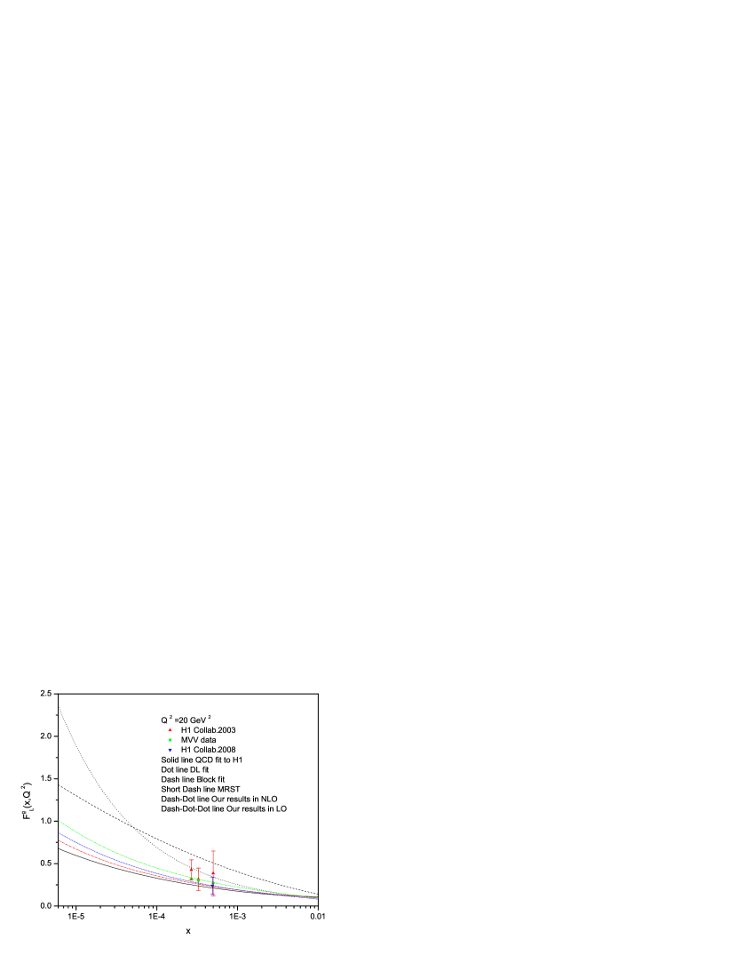
Figure 1:

Figure 2: