The ratio of the charm structure functions $F_{k}^{c}(k=2,L)$ at low-$x$ in DIS with respect to the expansion method

Abstract

We study the expansion method to the gluon distribution function at low $x$ values and calculate the charm structure functions in LO and NLO analysis. Our results provide compact formula for the ratio $R^{c}=\frac{F_{L}^{c}}{F^{c}_{2}}$ that is approximately independent of $x$ and the details of the parton distribution function at low $x$ values. This ratio could be good probe of the charm structure function $F^{c}_{2}$ in the proton from the reduced charm cross sections at DESY HERA. These results show that the charm structure functions obtained are in agreement with HERA experimental data and other theoretical models.

.1 Introduction

The low- $x$ regime of the quantum Cheromodynamic (QCD) has been intensely investigated in recent years for consideration of the heavy quarks [1-5]. Of course the notation of the intrinsic charm content of the proton has been introduced over 30 years ago in Ref.[6]. The study of production mechanisms of heavy quarks provides us with new tests of QCD. As in perturbative QCD (pQCD), physical quantities can be expanded into the strong coupling constant $\alpha_{s}(\mu^{2})$. Extensive the $\mu$ scale to the large values establish the theoretical analysis as can be described with hard processes. In the case of heavy quark production, we can have condition that the heavy quarks produced from the boson- gluon fusion (BGF) according to Fig.1. That is, in PQCD calculations the production of heavy quarks at HERA proceeds dominantly via the direct BGF where the photon interacts with a gluon from the proton by the exchange of a heavy quark pair.

In this processes all quark flavours lighter than charm are treated as massless with massive charm being produced dynamically in BGF. Charm production contributes to the total deep inelastic scattering (DIS) cross section by at most $30\%$ at HERA [7]. In the recent measurements of HERA [8], the charm contribution to the structure function at small $x$ is a large fraction of the total. This behavior is directly related to the growth of the gluon density at small $x$, as gluons couple only through the strong interaction. Consequently the gluons are not directly probed in DIS, only contributing indirectly via the $g{\rightarrow}q\bar{q}$ transition. This involves the computation of the BGF process $\gamma^{\star}g{\rightarrow}c\bar{c}$. This process can be created when the squared invariant mass of the hadronic final state is $W^{2}{\geq}4m_{c}^{2}$.
In this paper we apply the expansion of the gluon distribution at an arbitrary point to the charm structure functions in deep inelastic scattering. Then we present the ratio of the charm structure functions, that is independent of the gluon distribution and its useful to extract the charm structure function from the reduced charm cross section experimental data.

.2 Charm components of the structure functions

In deeply inelastic electron- proton scattering, the heavy- quark contribution to heavy flavor is according to this reaction

$$e(l_{1})+P(p){\rightarrow}e(l_{2})+Q(p_{1})\overline{Q}(p_{2})+X.$$ (1)

Here, neglecting the contribution of Z- boson exchange and omitting charged- current interactions. The deeply inelastic electroproduction cross section for the heavy quark-antiquark in the final sate can be written as

$$\frac{d^{2}\sigma^{c\overline{c}}}{dxdQ^{2}} = \frac{2{\pi}\alpha^{2}}{xQ^{4}}(1+(1-y)^{2})F_{2}(x,Q^{2},m_{c}^{2})$$

$$\times[1-\frac{y^{2}}{1+(1-y)^{2}}R^{c}],$$

where $R^{c}$ denotes the ratio of the charm structure functions and the kinematic variables are defined by $x=\frac{Q^{2}}{2p.q},y=\frac{p.q}{p.l}$ and $Q^{2}=-q^{2}$.

The deeply inelastic charm structure functions ($F_{k}(x,Q^{2},m_{c}^{2})$ for $k=2,L$) in the cross section (2) is given by [9]

$$F_{k}^{c}(x,Q^{2},m^{2}_{c})=2xe_{c}^{2}\frac{\alpha_{s}(\mu^{2})}{2\pi}\int_{ax}^{1}\frac{dy}{y}C_{g,k}(\frac{x}{y},\zeta)g(y,\mu^{2}),$$ (3)

where $a=1+4\zeta(\zeta{\equiv}\frac{m_{c}^{2}}{Q^{2}})$, $g(x,\mu^{2})$ is the gluon density and the mass factorization scale $\mu$, which has been put equal to the renormalization scale, is assumed to be either $\mu^{2}=4m_{c}^{2}$ or $\mu^{2}=4m_{c}^{2}+Q^{2}$. Here $C^{c}_{g,k}$ is the charm coefficient function in LO and NLO analysis as

$$C_{k,g}(z,\zeta) {\rightarrow} C^{0}_{k,g}(z,\zeta)+a_{s}(\mu^{2})[C_{k,g}^{1}(z,\zeta)$$

$$+\overline{C}_{k,g}^{1}(z,\zeta)ln\frac{\mu^{2}}{m_{c}^{2}}],$$

where $a_{s}(\mu^{2})=\frac{\alpha_{s}(\mu^{2})}{4\pi}$ and in the NLO analysis

$$\alpha_{s}(\mu^{2})=\frac{4{\pi}}{\beta_{0}ln(\mu^{2}/\Lambda^{2})}-\frac{4\pi\beta_{1}}{\beta_{0}^{3}}\frac{lnln(\mu^{2}/\Lambda^{2})}{ln(\mu^{2}/\Lambda^{2})}$$ (5)

with $\beta_{0}=11-\frac{2}{3}n_{f},\beta_{1}=102-\frac{38}{3}n_{f}$ ($n_{f}$ is the number of active flavours).

In the LO analysis, the coefficient functions BGF can be found [9], as

$$C^{0}_{g,2}(z,\zeta) = \frac{1}{2}([z^{2}+(1-z)^{2}+4z\zeta(1-3z)-8{\zeta^{2}}z^{2}]$$ (6)

$${\times}ln\frac{1+\beta}{1-\beta}+{\beta}[-1+8z(1-z)$$

$$-4z{\zeta}(1-z)]),$$

and

$$C^{0}_{g,L}(z,\zeta)=-4z^{2}{\zeta}ln\frac{1+\beta}{1-\beta}+2{\beta}z(1-z),$$ (7)

where $\beta^{2}=1-\frac{4z\zeta}{1-z}$.
At NLO, $O(\alpha_{em}\alpha_{s}^{2})$, the contribution of the photon- gluon component is usually presented in terms of the coefficient functions $C_{k,g}^{1},\overline{C}_{k,g}^{1}$. Using the fact that the virtual photon- quark(antiquark) fusion subprocess can be neglected, because their contributions to the heavy-quark leptoproduction vanish at LO and are small at NLO [1,10]. In a wide kinematic range, the contributions to the charm structure functions in NLO are not positive due to mass factorization and are less than $\%10$. Therefore the charm structure functions are dependence to the gluonic observable in LO and NLO. The NLO coefficient functions are only available as computer codes[9,10]. But in the high- energy regime ($\zeta<<1$) we can used the compact form of these coefficients according to the Refs.[11,12].

.3 The method

Now we want to calculate the charm structure functions by using the expansion method for the gluon distribution function. As can be seen, the dominant contribution to the charm structure functions comes from the gluon density at small $x$, regardless of the exact shape of the gluon distribution. Substitute $y=\frac{x}{1-z}$ in Eq.3 to obtain the more useful form, as

$$F_{k}^{c}(x,Q^{2},m^{2}_{c}) = 2e_{c}^{2}\frac{\alpha_{s}(\mu^{2})}{2\pi}\int_{1-\frac{1}{a}}^{1-x}dzC_{g,k}^{c}(1-z,\zeta)$$ (8)

$${\times}G(\frac{x}{1-z},\mu^{2}),$$

here $G(x)=xg(x)$ is the gluon distribution function. The argument $\frac{x}{1-z}$ of the gluon distribution in Eq.8 can be expanded at an arbitrary point $z=\alpha$ as

$$\frac{x}{1-z}|_{z=\alpha}=\frac{x}{1-\alpha}\sum_{k=1}^{\infty}[1+\frac{(z-\alpha)^{k}}{(1-\alpha)^{k}}].$$ (9)

The above series is convergent for $|z-\alpha|<1$. Using this expression we can rewrite and expanding the gluon distribution $G(\frac{x}{1-z})$ as

$$G(\frac{x}{1-z}) = G(\frac{x}{1-\alpha})$$

$$+\frac{x}{1-\alpha}(z-\alpha)\frac{{\partial}G(\frac{x}{1-a})}{{\partial}x}+O(z-\alpha)^{2}.$$

Retaining terms only up to the first derivative in the expansion and doing the integration, we obtain our master formula as

$$F_{k}^{c}(x,Q^{2},m^{2}_{c})=2e_{c}^{2}\frac{\alpha_{s}(\mu^{2})}{2\pi}A_{k}(x)$$

$${\times}G(\frac{x}{1-\alpha}(1-\alpha+\frac{B_{k}(x)}{A_{k}(x)})),$$ (11)

where

$$A_{k}(x)=\int_{1-\frac{1}{a}}^{1-x}C_{g,k}^{c}(1-z,\zeta)dz,$$ (12)

and

$$B_{k}(x)=\int_{1-\frac{1}{a}}^{1-x}(z-\alpha)C_{g,k}^{c}(1-z,\zeta)dz.$$ (13)

where $C_{g,k}^{c}$ is defined at Eq.4 in LO and NLO analysis and also $\alpha$ has an arbitrary value $0{\leq}\alpha{<}1$. Eq.10 can be rewritten as

$$F_{k}^{c}(x,Q^{2},m^{2}_{c})=2e_{c}^{2}\frac{\alpha_{s}(\mu^{2})}{2\pi}\eta_{k}G(\frac{x}{1-\alpha}({\beta_{k}}-\alpha),\mu^{2}).$$ (14)

This result shows that the charm structure functions $F_{k}^{c}(x,Q^{2})$ at $x$ are calculated using the gluon distribution at $\frac{x}{1-\alpha}(\beta_{k}-\alpha)$. Therefore, the gluon distribution at $\frac{x}{1-\alpha}(\beta_{k}-\alpha)$ can be simply extracted the charm structure functions ($F_{2}^{c}$ and $F_{L}^{c}$) in the low $x$ values according to the coefficients at the limit $x{\rightarrow}0$, in Table 1. Moreover, there is a directly relation between the charm structure functions and gluon distribution via the well known Bethe- Heitler process $\gamma^{\star}g{\rightarrow}c\bar{c}$.

Now, we defining the ratio of the charm structure functions and using Eq.14, we obtain the following equation

$$R^{c}=\frac{\eta_{L}}{\eta_{2}}\frac{G(\frac{x}{1-\alpha}(\beta_{L}-\alpha)}{G(\frac{x}{1-\alpha}(\beta_{2}-\alpha)}.$$ (15)

We observe that the right-hand side of this ratio is independent of $x$ and independent of the gluon distribution input according to the coefficients in Table 1. As in the low $x$ range we have

$$R^{c}{\approx}\frac{\eta_{L}}{\eta_{2}},$$ (16)

which is very useful to extract the charm structure function $F_{2}^{c}(x,Q^{2})$ from measurements of the doubly differential cross section of inclusive deep inelastic scattering at DESY HERA, independent of the gluon distribution function. Therefore, we can determine the charm structure function into the reduced cross section from the double- differential charm cross section as

$$F_{2}(x,Q^{2},m_{c}^{2})=\widetilde{\sigma}^{c\overline{c}}(x,Q^{2})/[1-\frac{y^{2}}{1+(1-y)^{2}}R^{c}].$$ (17)

Where $R^{c}$ is defined at Eq.16 and Table 1 and $\widetilde{\sigma}^{c\overline{c}}$ is taking from Ref.13, also the error bars in our determination can be examined by the following expression (Table 1)

$$\delta_{F_{2}^{c\overline{c}}}=F_{2}^{c\overline{c}}[\frac{\delta_{\widetilde{\sigma}^{c\overline{c}}}}{\widetilde{\sigma}^{c\overline{c}}}+\frac{\frac{y^{2}}{1+(1-y)^{2}}\delta_{R^{c}}}{1-\frac{y^{2}}{1+(1-y)^{2}}R^{c}}].$$ (18)

.4 Results and Discussion

For the calculation of the charm structure functions ($F_{2}^{c\overline{c}}$ and $F_{L}^{c\overline{c}}$), we choose $\Lambda=0.224GeV$, $m_{c}=1.5GeV$ and known that the dominant uncertainty in the QCD calculations arises from the uncertainty in the charm quark mass. Since the contribution of the longitudinal charm structure function to the DIS charm cross section (i.e., Eq.(2)) is proportional to $y^{2}$, so that the $F_{2}^{c\overline{c}}$ term dominates at $y\leq{0.08}$ and the relation $\widetilde{\sigma}^{c\overline{c}}=F_{2}^{c\overline{c}}$ holds to a very good approximation. Thus the contribution of the second term of the right hand Eq.(2) can be sizeable only at $y>{0.08}$. Therefore, for $y>{0.08}$, the ratio of the charm structure functions is very useful. In Fig.2 we observe that this ratio is according to results Refs.4 and 11 at low $x$. Also at NLO analysis its decrease as $Q^{2}$ increases and this is familiar from the Callan- Gross ratio. As we can see in this figure, this ratio has value $0.1<R^{c}<0.2$ in a wide region of $Q^{2}$.
We now extract $F_{2}^{c\overline{c}}$ from the H1 measurements of the reduced charm cross section [13] in Eq.17 with respect to Eq.16 for $Q^{2}{\geq}8.5GeV^{2}$. Our NLO results for the charm structure function are presented in Table 2, where they are compared with the experimental values from H1 data and they are comparable with the HVQDIS and CASCADE programs [14,15] as we can see at Table 11 in Ref.13(arXiv:1106.1028v1 [hep-ex] 6 Jun 2011). The error bars in Table 2 are according to the theoretical uncertainty related to the freedom in the choice of the renormalization scales in the ratio of the charm structure function and also the experimental total errors related to the results in Ref.13 according to the Eq.18. A comparison between our obtained values for the charm structure function and the existing data, indication the fact that the ratio $R^{c}$ can be determined with reasonable precision at any $y$ value.

In order to test the validity and correctness of our obtained charm structure functions with respect to the gluon distribution function (Eq.14), we obtained the charm structure functions into the gluon distribution input, which is usually taken from NLOGRV [9] or Block [16] parameterizations. As the gluon distribution input is dependent to a point of expansion $\alpha$. In order to estimate the theoretical uncertainty resulting from this, we choose $\alpha=0$ and $\alpha=0.8$ in the renormalization scale $\mu^{2}=4mc^{2}+Q^{2}$. In Figs.3-6, we observe that the theoretical uncertainty related to the freedom in the choice of $\alpha$ is very small at the renormalization scales. As can be seen in Figs.3-4, the better choice of the expansion point for the charm structure function $F_{2}^{c}$ is at the point $\alpha{\simeq}0.5$, as this point is favoured according to the current data. This means that in this kinematical region the longitudinal momentum of the gluon $x_{g}$ is more than three times the value of the longitudinal momentum of the probed charm quark- anitquark in BGF process. We compared our results for the charm structure function to the DL model [17-19], H1 data [13] and color dipole model [20]. In Figs.5-6, the better choice of the expansion point for the longitudinal charm structure function $F_{L}^{c}$ is $\alpha{\geq}0.8$, as compared only to the color dipole model [20]. As can be seen in these figures, the increase of our results for the charm structure functions $F^{c}_{k}(x,Q^{2})$ towards low $x$ are consistent and comparable with the experimental data and theoretical models.

.5 Conclusion

In summary, we have used the expansion method for the low $x$ gluon distribution and derived a compact formula for the ratio $R^{c}=\frac{F_{L}^{c\overline{c}}}{F_{2}^{c\overline{c}}}$ of the charm structure functions at NLO analysis. We observed that the this ratio is independent of $x$ and independent of the parton distribution function input, and also its useful to extract the charm structure function from the reduced charm cross section. Based upon of the reduced charm cross section in the low $x$ region, an approximate method for the calculation of the charm structure function $F_{2}^{c\overline{c}}$ is presented. Careful investigation of our results show a good agreement with the recent published charm structure functions $F_{2}^{c\overline{c}}$ and other theoretical models within errors from the expansion point and the renormalization scales.

References
1. A.Vogt, arXiv:hep-ph:9601352v2(1996).
2. H.L.Lai and W.K.Tung, Z.Phys.C74,463(1997).
3. A.Donnachie and P.V.Landshoff, Phys.Lett.B470,243(1999).
4. N.Ya.Ivanov, Nucl.Phys.B814, 142(2009); N.Ya.Ivanov and B.A.Kniehl, Eur.Phys.J.C59, 647(2009).
5. F.Carvalho, et.al., Phys.Rev.C79, 035211(2009).
6. S.J.Brodsky, P.Hoyer, C.Peterson and N.Sakai,Phys.Lett.B93, 451(1980); S.J.Brodsky, C.Peterson and N.Sakai, Phys.Rev.D23, 2745(1981).
7. K.Lipta, PoS(EPS-HEP)313,(2009).
8. C. Adloff et al. [H1 Collaboration], Z. Phys. C72, 593 (1996); J. Breitweg et al. [ZEUS Collaboration], Phys. Lett. B407, 402 (1997); C. Adloff et al. [H1 Collaboration], Phys. Lett. B528, 199 (2002); S. Aid et. al., [H1 Collaboration], Z. Phys. C72, 539 (1996); J. Breitweg et. al., [ZEUS Collaboration], Eur. Phys. J. C12, 35 (2000); S. Chekanov et. al., [ZEUS Collaboration], Phys. Rev. D69, 012004 (2004); Aktas et al. [H1 Collaboration], Eur. Phys.J. C45, 23 (2006); F.D. Aaron et al. [H1 Collaboration],Eur.Phys.J.C65,89(2010).
9. M.Gluk, E.Reya and A.Vogt, Z.Phys.C67, 433(1995); Eur.Phys.J.C5, 461(1998).
10. E.Laenen, S.Riemersma, J.Smith and W.L. van Neerven, Nucl.Phys.B 392, 162(1993).
11. A. Y. Illarionov, B. A. Kniehl and A. V. Kotikov, Phys. Lett.  B 663, 66 (2008).
12. S. Catani, M. Ciafaloni and F. Hautmann, Preprint CERN-Th.6398/92, in Proceeding of the Workshop on Physics at HERA (Hamburg, 1991), Vol. 2., p. 690; S. Catani and F. Hautmann, Nucl. Phys. B 427, 475(1994); S. Riemersma, J. Smith and W. L. van Neerven, Phys. Lett. B 347, 143(1995).
13. F.D.Aaron, et.al,. H1 Collab., Phys.Lett.b665,139(2008); Eur.Phys.J.C71, 1509(2011); Eur.Phys.J.C71, 1579(2011); arXiv:1106.1028v1 [hep-ex] 6 Jun 2011; arXiv:0911.3989v1 [hep-ex] 20 Nov 2009.
14. H. Jung, CASCADE V2.0, Comp. Phys. Commun. 143, 100(2002).
15. B.W. Harris and J. Smith, Nucl. Phys. B452, 109(1995); Phys. Rev. D57, 2806(1998).
16. M.M.Block, L.Durand and D.W.Mckay, Phys.Rev.D77, 094003(2008).
17. A.Donnachie and P.V.Landshoff, Z.Phys.C 61, 139(1994); Phys.Lett.B 518, 63(2001); Phys.Lett.B 533, 277(2002); Phys.Lett.B 470, 243(1999); Phys.Lett.B 550, 160(2002).
18. R.D.Ball and P.V.landshoff, J.Phys.G26, 672(2000).
19. P.V.landshoff, arXiv:hep-ph/0203084 (2002).
20. N.N.Nikolaev and V.R.Zoller, Phys.Lett. B509, 283(2001).

.6 Figure captions

Fig.1: The photon- gluon fusion.

Fig.2: The ratio $R^{c}$ evaluated as function of $Q^{2}$ at NLO analysis from Eq.16. The error bars are the theoretical uncertainty using the renormalization scales $\mu^{2}=4m_{c}^{2}$ and $\mu^{2}=4m_{c}^{2}+Q^{2}$.

Fig.3: The charm structure function ($F_{2}^{c\overline{c}}$) obtained at $Q^{2}=20GeV^{2}$ with respect to the input gluon distribution NLO-GRV parametermization [9] (Solid line according to the expanding point $\alpha=0$ and Dash-Dot line according to the expanding point $\alpha=0.8$) compared with DL fit[17-19] (Dot line), color dipole model [20] (Dash line) and H1 data [13] (square) that accompanied with total errors at the renormalization scale $\mu^{2}=4m_{c}^{2}+Q^{2}$.

Fig.4: The charm structure function ($F_{2}^{c\overline{c}}$) obtained at $Q^{2}=20GeV^{2}$ with respect to the input gluon distribution Block fit [16] (Solid line according to the expanding point $\alpha=0$ and Dash-Dot line according to the expanding point $\alpha=0.8$) compared with DL fit[17-19] (Dot line), color dipole model [20] (Dash line) and H1 data [13] (square) that accompanied with total errors at the renormalization scale $\mu^{2}=4m_{c}^{2}+Q^{2}$.

Fig.5: The longitudinal charm structure function ($F_{L}^{c\overline{c}}$) obtained at $Q^{2}=20GeV^{2}$ with respect to the input gluon distribution NLO-GRV parametermization [9] (Solid line according to the expanding point $\alpha=0$ and Dash-Dot line according to the expanding point $\alpha=0.8$) compared with the color dipole model [20] (Dash line) at the renormalization scale $\mu^{2}=4m_{c}^{2}+Q^{2}$.

Fig.6: The longitudinal charm structure function ($F_{L}^{c\overline{c}}$) obtained at $Q^{2}=20GeV^{2}$ with respect to the input gluon distribution Block fit [16] (Solid line according to the expanding point $\alpha=0$ and Dash-Dot line according to the expanding point $\alpha=0.8$) compared with the color dipole model [20] (Dash line) at the renormalization scale $\mu^{2}=4m_{c}^{2}+Q^{2}$.

Figure 1:

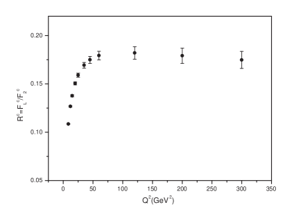
Figure 2:

Table 1: The constant values in this analysis at $Q^{2}$ values in the limit $x{\rightarrow}0$.

$Q^{2}(GeV^{2})$	$\eta_{2}$	$\delta_{\eta_{2}}$	$\beta_{2}$	$\delta_{\beta_{2}}$	$\eta_{L}$	$\delta_{\eta_{L}}$	$\beta_{L}$	$\delta_{\beta_{L}}$	$R^{c}$	$\delta_{R^{c}}$
8.5	0.4645	1.95E-3	1.8393	2E-4	0.0504	4E-4	1.7853	1E-4	0.1085	4.5E-4
12	0.5763	3.7E-3	1.8083	3.5E-4	0.0730	9E-4	1.7453	1.5E-4	0.1267	8E-4
15	0.6546	5.45E-3	1.7883	5E-4	0.0901	1.45E-3	1.7200	1E-4	0.1377	1.1E-3
20	0.7611	8.45E-3	1.7632	7E-4	0.1145	2.45E-3	1.6883	2E-4	0.1505	1.6E-3
25	0.8469	0.0114	1.7447	1E-3	0.1347	3.6E-3	1.6654	2.5E-4	0.1590	2.1E-3
35	0.9795	0.0173	1.7190	1.35E-3	0.1659	5.8E-3	1.6343	3E-4	0.1693	2.9E-3
45	1.0800	0.0227	1.7016	1.65E-3	0.189	7.9E-3	1.6139	3.5E-4	0.1749	3.6E-3
60	1.1953	0.0300	1.6838	2.05E-3	0.2144	0.0107	1.5936	3.5E-4	0.1793	4.45E-3
120	1.4709	0.052	1.6500	3.1E-3	0.2681	0.019	1.5568	3.5E-4	0.1820	6.5E-3
200	1.6698	0.0718	1.6307	3.85E-3	0.2996	0.026	1.5387	3E-4	0.1791	7.85E-3
300	1.8252	0.089	1.6187	4.3E-3	0.3198	0.0316	1.5283	2E-4	0.1748	8.8E-3

Table 2: The charm structure function determined based on the reduced charm cross section data that accompanied with errors.

$Q^{2}(GeV^{2})$	$x$	$y$	$\widetilde{\sigma}^{c\overline{c}}$	$\delta_{\widetilde{\sigma}^{c\overline{c}}}(\%)$	$F_{2}^{c\overline{c}}$(Ref.13)	$\delta_{F_{2}^{c\overline{c}}}(\%)$	$F_{2}^{c\overline{c}}$(Our Results)	$\delta_{F_{2}^{c\overline{c}}}$
8.5	0.00050	0.167	0.176	14.8	0.176	1.0	0.1763	14.8
8.5	0.00032	0.262	0.186	15.5	0.187	1.0	0.1869	15.6
12	0.00130	0.091	0.150	18.7	0.150	1.0	0.1501	18.7
12	0.00080	0.148	0.177	15.9	0.177	1.1	0.1773	15.9
12	0.00050	0.236	0.240	11.2	0.242	1.0	0.2441	11.4
12	0.00032	0.369	0.273	13.8	0.277	1.1	0.2764	14.0
20	0.00200	0.098	0.187	12.7	0.188	1.1	0.1871	12.7
20	0.00130	0.151	0.219	11.9	0.219	1.1	0.2194	11.9
20	0.00080	0.246	0.274	10.2	0.276	1.0	0.2756	10.3
20	0.00050	0.394	0.281	13.8	0.287	1.1	0.2859	14.0
35	0.00320	0.108	0.200	12.7	0.200	1.1	0.2002	12.7
35	0.00200	0.172	0.220	11.8	0.220	1.0	0.2206	11.8
35	0.00130	0.265	0.295	9.70	0.297	1.0	0.2973	9.8
35	0.00080	0.431	0.349	12.7	0.360	1.1	0.3575	13.0
60	0.00500	0.118	0.198	10.8	0.199	1.1	0.1983	10.8
60	0.00320	0.185	0.263	8.40	0.264	1.0	0.2640	8.5
60	0.00200	0.295	0.335	8.80	0.339	1.0	0.3385	8.9
60	0.00130	0.454	0.296	15.1	0.307	1.0	0.3047	15.6
120	0.01300	0.091	0.133	14.1	0.133	1.2	0.1331	14.1
120	0.00500	0.236	0.218	11.1	0.220	1.1	0.2194	11.2
120	0.00200	0.591	0.351	12.8	0.375	2.9	0.3712	13.6
200	0.01300	0.151	0.161	11.9	0.160	2.7	0.1604	11.9
200	0.00500	0.394	0.237	13.5	0.243	2.9	0.2419	13.8
300	0.02000	0.148	0.117	18.5	0.117	2.9	0.1173	18.5
300	0.00800	0.369	0.273	12.7	0.278	2.9	0.2777	12.9

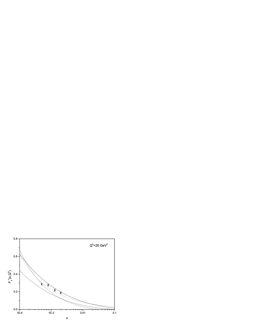
Figure 3:

Figure 4:

Figure 5:

Figure 6: