Automated Classification of Periodic Variable Stars detected
by the Wide-field Infrared Survey Explorer
Abstract
We describe a methodology to classify periodic variable stars identified using photometric time-series measurements constructed from the Wide-field Infrared Survey Explorer (WISE) full-mission single-exposure Source Databases. This will assist in the future construction of a WISE Variable Source Database that assigns variables to specific science classes as constrained by the WISE observing cadence with statistically meaningful classification probabilities. We have analyzed the WISE light curves of 8273 variable stars identified in previous optical variability surveys (MACHO, GCVS, and ASAS) and show that Fourier decomposition techniques can be extended into the mid-IR to assist with their classification. Combined with other periodic light-curve features, this sample is then used to train a machine-learned classifier based on the random forest (RF) method. Consistent with previous classification studies of variable stars in general, the RF machine-learned classifier is superior to other methods in terms of accuracy, robustness against outliers, and relative immunity to features that carry little or redundant class information. For the three most common classes identified by WISE: Algols, RR Lyrae, and W Ursae Majoris type variables, we obtain classification efficiencies of 80.7%, 82.7%, and 84.5% respectively using cross-validation analyses, with 95% confidence intervals of approximately 2%. These accuracies are achieved at purity (or reliability) levels of 88.5%, 96.2%, and 87.8% respectively, similar to that achieved in previous automated classification studies of periodic variable stars.
1 Introduction
The Wide-field Infrared Survey Explorer (WISE; Wright et al., 2010) mapped the entire sky in four bands centered at wavelengths of 3.4, 4.6, 12, and 22 m (hereafter W1, W2, W3, and W4) from January 7, 2010 to February 1, 2011 that spanned both cryogenic and post-cryogenic phases. WISE conducted its survey from a sun-synchronous polar orbit using a 40 cm cryogenically cooled telescope equipped with four 1024 1024 infrared (IR) array detectors that simultaneously imaged the same 47′ 47′ field-of-view in all bands. The WISE survey strategy alternated stepping the scan path forward and backward on subsequent orbits in an asymmetric pattern that approximately matched the per day orbital precession rate. In this way, each point near the ecliptic plane was observed on every other orbit, or every 191 minutes, yielding typically 12 independent exposures over one day. The number of exposures increases with ecliptic latitude, reaching over 6000 at the ecliptic poles.
WISE surveyed the sky approximately 1.5 times during its cryogenic phase that ended on September 29, 2010. Data continued to be collected for another four months to support the discovery of Near Earth Objects (the NEOWISE program; Mainzer et al., 2011). During this post-cryogenic phase, 70% of the sky was scanned, with only the W1 and W2 detectors returning scientifically useful data. Overall, WISE covered the full sky slightly more than twice, with each sky-coverage separated by approximately six months. When all the mission data are combined, the median single-exposure depth-of-coverage on the ecliptic becomes and the effective observation timespan (without the six month phase shift) days.
The WISE Single-Exposure Source Databases (Cutri et al., 2012) contain the photometry from each individual WISE exposure. These offer a unique opportunity to search for variable stars over the entire sky at wavelengths that are relatively immune to dust extinction. In particular, the most common pulsational variables (e.g., Cepheids, RR Lyrae, and Miras) have served as standard candles that enabled measurements of the size scale of the Milky Way and the Universe (e.g., Tammann et al., 2008). Products from previous WISE data releases have already had a significant impact on the calibration of the RR Lyrae period-luminosity relation at mid-IR wavelengths (Klein et al., 2011; Madore et al., 2013; Dambis et al., 2014; Klein et al., 2014). An all-sky census of pulsating variables offers an opportunity to improve our understanding of Milky Way tomography and the distribution of dark matter in the Galaxy through their association with relic streams from disrupted star clusters and dwarf galaxies (Grillmair, 2010). Pulsational variables are also crucial for understanding stellar birth, structure, mass loss, and evolution (Eyer & Mowlavi, 2008). On the other hand, variability associated with eclipsing binaries (e.g., Algol, Lyrae, and W Ursae Majoris types) provide laboratories for probing accretion, mass transfer, binary evolution, and exoplanets (for a review, see Percy, 2007).
The deluge of data from current and future time-domain surveys presents an enormous challenge for human-based vetting, classification, and follow-up. Fortunately, computers and efficient machine-learning (ML) algorithms are starting to revolutionize the taxonomic problem. A broad class of ML methods are generically referred to as “supervised”. These methods entail defining a set of rules or models that best describe the relationship between the properties (features) of a data set and some known outcomes (e.g., classifications), and then using this “trained” mapping to predict the outcomes for new data. On the other hand, “unsupervised” methods attempt to blindly identify patterns and structures amongst the features of a data set, that is, with no pre-labelled classes or outcomes to learn from. For an overview of ML methods in general, see Hastie et al. (2009). For a review of ML applications in astronomy, see Ball & Brunner (2010). ML also provides a statistical framework to make probabilistic statements about the class(es) that a particular object with a set of observables or features could belong to. Given the same training model, these statements are also reproducible and deterministic, whereas a human-based classification approach is not.
Supervised ML techniques have gained considerable popularity in the automated classification of variable stars (Woźniak et al., 2004; Eyer & Blake, 2005; Debosscher et al., 2007; Mahabal et al., 2008; Blomme et al., 2010; Richards et al., 2011). In particular, Richards et al. (2011) compared several classification frameworks for variable stars selected from multiple surveys and concluded that the random forest ML classifier (a tree-based technique popularized by Breiman, 2001) generally performed best. Due to their flexibility and robustness, random forests have also attained popularity in the real-time discovery and classification of astronomical transients in general (e.g., Bloom et al., 2012; Morgan et al., 2012; Brink et al., 2013). Guided by its success, we adopt the random forest method as the primary ML classifier in this study.
The WISE All-Sky Release Source Catalog (Cutri et al., 2012) contains approximately 8 million sources where likely flux variables were flagged using a methodology similar to that described in Hoffman et al. (2012). We are in the process of constructing the WISE Variable Source Database (WVSDB) that builds upon this basic variability flagging in the Catalog. This database will contain confirmed variable sources with their light curves, derived properties such as periods and amplitudes, and where appropriate, the probabilities of belonging to specific known variability classes.
The first step towards the construction of the WVSDB is a framework that can automatically and probabilistically classify variables using features and diagnostics derived from the WISE single-exposure time-series measurements. This paper describes the methodology behind this framework, starting with the construction of a training (or “truth”) sample leveraged on known variables classified in previous optical surveys and cross-matched to WISE to define robust mid-IR light curve features for classification. In particular, we show how Fourier decomposition techniques can be extended into the mid-IR to define the relevant features for discriminating between the various classes. This training sample is then used to fit and validate the popular random forest machine-learning technique to assist with the future classification of WISE flux variables for the WVSDB.
This paper is organized as follows. In Section 2 we define the variability classes that WISE is most sensitive to. Section 3 describes the construction of the training sample and selection of the mid-IR light curve features. An analysis of these features for the various classes of interest is presented in Section 4. The random forest machine-learning method for automated classification is described and evaluated in Section 5, where we also compare this method to other state-of-the-art machine-learning methods. Section 6 gives an overview of the WVSDB, the classification plan, and how a feedback mechanism based on “active-learning” could be used to allow for selection biases in the input training sample. Results are summarized in Section 7.
2 Classification Scheme
The WISE full mission baseline and observing cadence is well-suited for studying periodic variable stars with periods of days, where 3 days is approximately the maximum period that can be recovered using our period estimation technique (Section 3.2) for light curves constructed from observations within a few tens of degrees of the ecliptic. The most common variables in this category are RR Lyrae (RR Lyr) pulsational variables and Algol, Lyrae, and W Ursae Majoris (W UMa) eclipsing binaries. Optical surveys generally find W UMa variables (a class of contact binaries) to be the most abundant, comprising 95% of all variable stars in the solar neighborhood (Eggen, 1967; Lucy, 1968). Despite their small variability amplitudes and relatively weak emission in the mid-infrared, WISE is sensitive to the brightest W UMa variables at the high end of the amplitude distribution. Lyrae eclipsing binaries are a class of semi-detached binary stars where one member of the pair fills the Roche lobe of the other. Previous optical studies have shown that Lyrae are generally difficult to separate from Algol-type (detached) eclipsing binaries based on light-curve shape alone (Malkov et al., 2007; Hoffman et al., 2008). Our analyses of the WISE light curve features (Section 4) also show these variables to largely overlap with Algols, and also perhaps with W Uma variables to some extent. The degeneracies can only be resolved with supplementary spectral information. Therefore, we are left with three broad periodic variable star classes that are best suited for WISE’s observing constraints: Algols (with the inclusion of many Lyrae); W UMa; and RR Lyr.
Periodic variables that are not assigned to any of these three broad classes (according to some probability threshold; see Section 6) will be initially flagged as “unknown”; for example, Cepheid variables. They may be reclassified and associated with new classes (not in the initial training sample described in Section 3.1) if more objects with similar features are identified following a first classification pass. Subsequent classification passes will use refined training samples augmented with new classes using an “active-learning” approach. Details are given in Section 6.1.
3 Training Sample and Feature Selection
3.1 Training Sample Definition
In order to calibrate and validate a classification method for WISE light curves, we assembled a “truth” list of variable stars that were previously classified with measured periods from a number of optical variability surveys. This list includes all eclipsing binaries and RR Lyr stars in the General Catalogue of Variable Stars (GCVS; Samus, 2013); the MACHO Variable Star Database (Alcock, 2003), and the All-Sky Automated Survey (ASAS; Pojmanski, 2006). This list of known variables was then positionally cross-matched to the WISE All-Sky Source Catalog (Cutri et al., 2012). A match-radius tolerance of was used and the brightest WISE source was selected if multiple matches were present. Furthermore, only sources with a WISE Catalog variability flag (Cutri et al., 2012, section IV.4.c.iii) of in the W1 band were retained. This criterion ensured that the WISE source had a relatively good time-averaged photometric signal-to-noise ratio (with typically S/N in the W1 single-exposures) and a high likelihood of also being variable in the mid-IR. After cross-matching, 1320 objects were rejected because they were labeled as either ambiguous (assigned to two or more classes), uncertain, or had different classifications between the optical catalogs. A further 2234 objects had duplicate entries amongst the optical catalogs (assigned to the same class) and one member of each pair was retained. In the end, we are left with a training sample of 8273 known variables with WISE photometry. Of these 8273 objects, 1736 are RR Lyr, 3598 are Algol-type eclipsing binaries, and 2939 are W UMa-type eclipsing binaries according to classifications reported in previous optical variability surveys.
We assume here that the bulk of classifications reported in the ASAS, GCVS, and MACHO surveys (primarily those objects labeled as Algol, RR Lyr, or W Uma) are correct, or accurate enough as to not significantly affect the overall core-class definitions in the WISE parameter (feature) space. The removal of objects with ambiguous and uncertain classifications, or with discrepant classifications between the catalogs is expected to have eliminated the bulk of this uncertainty. A comparison of our classification performance to other studies that also used classifiers trained on similar optical catalogs (Section 5.6) shows that possible errors in the classification labels of the training sample are not a major source of uncertainty. However, these errors cannot be ignored.
There is no guarantee that the training sample described here represents an unbiased sample of all the variable types that WISE can recover or discover down to fainter flux levels and lower S/N ratios over the entire sky. This training sample will be used to construct an initial classifier to first assess general classification performance (Section 5.6). In future, this classifier will be used to initially classify WISE flux-variables into the three broad variability classes defined above. Inevitably, many objects will remain unclassified in this first pass. To mitigate training sample biases and allow more of the WISE-feature space to mapped and characterized, we will use an active-learning framework to iteratively refine the training sample as objects are accumulated and (re)classified. This will allow more classes to be defined as well as sharpen the boundaries of existing ones, hence alleviating possible errors in the input classification labels (see above). Details are discussed under our general classification plan in Section 6.
3.2 Mid-IR Light Curve Feature Generation
A requirement of any classification system is a link between the features used as input and the classes defined from them. We review here the seven mid-IR light curve features that we found work best at discriminating between the three broad classes that WISE is most sensitive to (defined in Section 2). These were motivated by previous variable star classification studies (e.g., Kinemuchi et al., 2006; Deb & Singh, 2009; Richards et al., 2011)
We first extracted the time-resolved mid-IR photometry and constructed light curves for all sources in our training sample from the WISE All-Sky, 3-Band, and Post-Cryo Single-Exposure Source Databases111http://irsa.ipac.caltech.edu/Missions/wise.html. Light curves were constructed using only the W1 band. This is because W1 generally has better sensitivity than W2 for the variable stars under consideration. For each source, a period was estimated using the generalized Lomb-Scargle periodogram (Zechmeister & Kürster, 2009; Scargle, 1982, see Section 4 for this choice). The light curves were phased to the highest peak in the periodogram that fell in the period range: 0.126 day ( 3 hours) to 10 days. The lower value corresponds to the characteristic WISE single-exposure sampling and the upper limit is based on the known periods of Algol-type binaries that could be recovered by WISE given the typical time-span of observations, with a generous margin. These recovered periods () constitute our first feature to assist with classification. Section 4 compares these estimates to the available periods derived from optical light curves.
The second feature derived from the WISE light curves in our training sample is the Stetson- variability index (Stetson, 1996; Kim et al., 2011). This index quantifies the degree of synchronous variability between two bands. Because the band W1 and W2 measurements generally have the highest S/N ratio for objects in the classes of interest, only these bands are used in the calculation of this index. The Stetson- index is the scaled product of the Stetson and indices:
| (1) |
Stetson- is a measure of the correlation between two bands (, ; or W1, W2 respectively) and is defined as
| (2) | |||||
| (3) | |||||
| (4) | |||||
| (5) |
where is the index for each data point, is the total number of points, sgn() is the sign of , is the photometric magnitude of flux measurement in band , and is its uncertainty. The Stetson- index is a measure of the kurtosis of the magnitude distribution and is calculated by collapsing a single-band light curve:
| (6) |
For a pure sinusoid, , while for a Gaussian magnitude distribution, . This is also the scaling factor in the -index (equation 1).
Our third derived feature is the magnitude ratio (; Kinemuchi et al., 2006). This measures the fraction of time a variable star spends above or below its median magnitude and is useful for distinguishing between variability from eclipsing binaries and pulsating variables. This is computed using the magnitude measurements for an individual band and is defined as
| (7) |
For example, if a variable star spends 50% of its time at near constant flux that only falls occasionally, . If its flux rises occasionally, . A star whose flux is more sinusoidal will have .
The remaining four features are derived from a Fourier decomposition of the W1 light curves. Fourier decomposition has been shown to be a powerful tool for variable star classification (Deb & Singh, 2009; Rucinski, 1993). To reduce the impact of noise and outliers in the photometric measurements, we first smooth a mid-IR light curve using a local non-parametric regression fit with Gaussian kernel of bandwidth () 0.05 days. We then fit a 5 order Fourier series to the smoothed light curve , parameterized as
| (8) |
where is the orbital phase at observation time relative to some reference time and is computed using our recovered period (see above) as
| (9) |
where “int” denotes the integer part of the quantity and . The parameters that are fit in equation (8) are the amplitudes and phases . The quantities that we found useful for classification (see section 4 with some guidance from Deb & Singh, 2009) are the two relative phases
| (10) |
| (11) |
and the absolute values of two Fourier amplitudes: and .
To summarize, we have a feature-vector consisting of seven metrics for each mid-IR light curve in our training sample: the recovered period , the magnitude ratio (equation 7), the Stetson- index (equation 1), and the four Fourier parameters: , , , and . Together with available class information from the literature (the dependent variable), we constructed a data matrix consisting of 8273 labeled points (“truth” samples) in a seven-dimensional space. Section 5 describes how this data matrix is used to train and validate a machine-learned classifier.
4 Preliminary Analysis of Features for Classification
Before using our training sample to construct an automated classification algorithm, we present here a qualitative analysis of the derived light-curve features across the three different classes of interest. That is, how well they perform individually and in combination, in a qualitative sense, for discriminating between classes. The relative feature importance across (and within) classes will be explored in more detail using metrics generated during the classifier-training phase in Section 5.5.
The accuracy of period recovery is an important factor in the classification process, in particular since this metric is also used (indirectly) to derive the features from Fourier decomposition. Given all three target classes overlap at least partially in period, it is important to minimize any period aliasing as much as possible, that is, any inadvertent phasing of the time-series data to an integer harmonic of the true period. The generalized Lomb-Scargle periodogram (GLS; Zechmeister & Kürster, 2009) was superior to other methods in recovering the correct period and minimizing period aliasing. The other methods we explored were the standard Lomb-Scargle algorithm; phase dispersion minimization method (PDM; Stellingwerf, 1978); multiharmonic analysis of variance (AOV; Schwarzenberg-Czerny, 1998); and the string-length algorithm (Lafler & Kinman, 1965). The GLS method recovered the correct period for the largest number of variables and minimized period aliasing (for mostly the RR Lyr class; see below). This is likely due to the relatively sparse temporal sampling of many WISE sources where GLS is most robust. GLS also has the advantage of incorporating measurement uncertainties in the calculation, whereas many other methods do not.
As shown in Figure 1, period recovery is good for periods of less than days. Longer periods are more difficult to recover from WISE data due to the observing cadence, as is evident by the increased scatter at longer periods. Nearly all the RR Lyr variables are recovered at the fundamental period, while the Algol and W UMa variables are recovered at half the period. This separation arises from the fact that eclipsing systems usually have two minima per cycle (the primary and seconday eclipses) while pulsating variable stars have only one. This half-period aliasing for the periods of eclipsing binaries does not impact their classification (or separability from pulsating variables in general) since we find they can be reliably distinguished using other features (see below). Thus, once an eclipsing binary has been identified using all the available light curve features, their measured period can be doubled to recover the correct period. One should also note several alias groupings in Figure 1, particularly for the W UMa class. These are due to the sinusoidal nature of their light curves and their relatively short periods ( day) where sparse-sampling of the WISE data can significantly affect period recovery.
Each feature in our seven-dimensional feature vector is compared against every other in Figure 2 for the three classes of interest in our training sample. There are 21 unique sets of feature pairs. This scatter-plot matrix provides both a qualitative sense of the degree of correlation between features as well as class separability in each two-dimensional projection. Feature correlations and possible redundancies are further explored in Section 5.2. The features that tend to separate the classes relatively well involve combinations of the Fourier amplitudes (, ) and relative phase parameters (, ), but the separation is also relatively strong in the -index versus magnitude ratio () plane. We expand on the details for three pairs of features below.
Figures 3 and 4 show the distribution of the Fourier amplitudes and relative phase parameters for each class. The RR Lyr and W UMa classes in particular appear to partially overlap in each 2-D plane formed by each pair of parameters. This is because many RR Lyr, especially those of the RRc subclass, have nearly sinusoidal light curves that are very similar to some W UMa variables. The periods of these two classes (Figure 1) also overlap to some extent. Figure 5 shows the benefit of including the magnitude ratio and Stetson -index to assist in distinguishing RR Lyr from the eclipsing binary (Algol and W UMa) classes in general, which may not be achieved using the Fourier amplitudes or phase parameters alone.
The Algol class appears to isolate itself rather well from the RR Lyr and W Uma classes in Figures 3 and 5, and only from the RR Lyr class in Figure 4. This is due to the asymmetrical nature of the Algol-type light curves and the fact that their primary and secondary minima are separated by an orbital phase of 0.5. This is common amongst Algol-type eclipsing binaries since most of them have orbital eccentricities of approximately zero. This also explains why there is a tight clump centered at and in Figure 4. There is however some small overlap between Algols and the RR Lyr and W UMa classes (which is smaller than that between the RR Lyr and W Uma classes). This primarily occurs for the shorter period Algols with similar depths in their primary and secondary eclipses, indicating the component stars are similar in nature. For these, the light curves become more sinusoidal and indistinguishable from the other classes.
From this preliminary exploratory analysis of the light curve features (using simple pairwise comparisons), it is clear that we need to explore class separability using the full joint seven-dimensional feature space, with some quantitative measure for assigning class membership. This is explored in the following sections. In particular, the relative feature importance is revisited and explored in more detail in Section 5.5.
5 Machine-Learned Supervised Classification Framework
The classes and their features defined above form the basis of a “supervised” classification framework. This method uses a sample of objects (here variable sources) with known classes to train or learn a non-parametric function (model) that describes the relationship between the derived features and these classes. This sample of labeled classes is referred to as the training sample. Our ultimate goal is to use this model to automatically predict the most probable class of future objects from its derived features, or in general, the probability that it belongs to each of the pre-defined classes. These probabilities quantify the degree to which a particular object could belong to specific class, therefore making the classification process less subjective, or more open to interpretation and further analysis. Section 5.4 describes how these probabilities are defined.
Many previous studies have used machine learning (ML) methods to classify variable stars from their photometric time series, in particular, in large surveys capable of identifying 20 or more variability classes. The intent has been to develop a generic classifier that is accurate, fast and robust, and can be used to classify objects from surveys other than those used to construct the classifier. Eyer et al. (2008), Richards et al. (2011), and Long et al. (2012) discuss some of the challenges on this front. The main challenge here is the presence of survey-dependent systematics, for example, varying cadence, flux sensitivity, signal-to-noise ratio, number of epochs, etc. This heterogeneity introduces systematic differences in the derived light-curve features, leading to biased training models and degraded classifier performance when attempting to classify new objects. A related issue is class-misrepresentation in the training model, i.e., where classes are inadvertently omitted because of limitations in the specific survey(s) used to construct the training sample. This will impact classifications for other surveys whose properties may allow these additional classes to be detected. Training a classifier using a subset of labeled (pre-classified) objects drawn from the same target sample for which bulk classifications are required (i.e., with similar properties) minimizes these biases, but does not eradicate them. Methods to mitigate training-sample biases for the classification of WISE flux-variables are discussed in Section 6.1.
Some of the ML methods used to classify variable stars include support vector machines (Woźniak et al., 2004; Debosscher et al., 2007), Kohonen self-organizing maps (Brett et al., 2004), Bayesian networks and mixture-models (Eyer & Blake, 2005; Mahabal et al., 2008), principle component analysis (Deb & Singh, 2009), multivariate Bayesian and Gaussian mixture models (Blomme et al., 2010, 2011) for the Kepler mission, and thick-pen transform methods (Park et al., 2013). Debosscher et al. (2007) explored a range of methods applied to several large surveys that included Hipparcos and OGLE: artificial neural networks, Bayesian networks, Gaussian mixture models, and support vector machines. All these methods appear to achieve some level of success; however, using the same input data, Richards et al. (2011) and Dubath et al. (2011) explored the performance of tree-based classification schemes that include random forests and found these to be generally superior to the methods in Debosscher et al. (2007) in terms of accuracy, robustness to outliers, ability to capture complex structure in the feature space, and relative immunity to irrelevant and redundant features.
Unlike the complex heterogeneous nature of the many-class/multi-survey classification problem noted above, the good overall homogeneity of the WISE survey provides us with a well-defined sample of uniformly sampled light-curves from which we can train and tune a ML classifier and use it for initial classification in future. As discussed in Section 3.1 and further in Section 6.1, these initial classifications will be used to refine the classifer and mitigate possible biases in the input training sample. Below, we focus on training and validating a random forest (RF) classifier, then compare its performance to some other state-of-the-art methods: artificial neural networks (NNET), -Nearest Neighbors (NN), and support vector machines (SVM). We do not delve into the details of these other methods, as our intent is simply to provide a cross-check with the RF classifier.
5.1 Classification using Trees and Random Forests
ML methods based on classification and regression trees (CART) were popularized by Breiman (1984). Decision trees are intuitive and simple to construct. They use recursive binary partitioning of a feature space by splitting individual features at values (or decision thresholds) to create disjoint rectangular regions – the nodes in the tree. The tree-building process selects both the feature and threshold at which to perform a split by minimizing some measure of the inequality in the response between the two adjacent nodes (e.g., the fractions of objects across all known classes, irrespective of class). The splitting process is repeated recursively on each subregion until some terminal node-size is reached (nodesize parameter below).
Classification trees are powerful non-parametric classifiers that can deal with complex non-linear structures and dependencies in the feature space. If the trees are sufficiently deep, they generally yield a small bias with respect to the true model that relates the feature space to the classification outcomes. Unfortunately, single trees do rather poorly at prediction since they lead to a high variance, e.g., as encountered when overfitting a model to noisy data. This is a consequence of the hierarchical structure of the tree: small differences in the top few nodes can produce a totally different tree and hence wildly different outcomes. Therefore, the classic bias versus variance tradeoff problem needs to be addressed. To reduce this variance, Breiman (1996) introduced the concept of bagging (bootstrap aggregation). Here, many trees ( of them) are built from randomly selected (bootstrapped) subsamples of the training set and the results are then averaged. To improve the accuracy of the final averaged model, the random forest (RF) method (Breiman, 2001) extends the bagging concept by injecting further randomness into the tree building process. This additional randomness comes from selecting a random subset of the input features ( parameter below) to consider in the splitting (decision) process at each node in an individual tree. This additional randomization ensures the trees are more de-correlated prior to averaging and gives a lower variance than bagging alone, while maintaining a small bias. These details may become clearer in section 5.4 where we outline the steps used to tune and train the RF classifier. For a more detailed overview, we refer the interested reader to ch.15 of Hastie et al. (2009) and Breiman & Cutler (2004).
Random forests are popular for classification-type problems and are used in many disciplines such as bioinformatics, Earth sciences, economics, genetics, and sociology. They are relatively robust against overfitting and outliers, weakly sensitive to choices of tuning parameters, can handle a large number of features, can achieve good accuracy (or minimal bias and variance), can capture complex structure in the feature space, and are relatively immune to irrelevant and redundant features. Furthermore, RFs include a mechanism to assess the relative importance of each feature in a trivial manner. This is explored in section 5.5. For our tuning, training, and validation analyses, we use tools from the R statistical software environment222R is freely-available at http://cran.r-project.org. In particular, we make extensive use of the caret (Classification and Regression Training) machine learning package (Kuhn, 2008), version 5.17-7, August 2013.
5.2 Feature Collinearity and Redundancy Checks
As mentioned earlier, the RF method is relatively immune to features that are correlated with any other feature or some linear combination of them, i.e., that show some level of redundancy in “explaining” the overall feature space. However, it is recommended that features that are strongly correlated with others in the feature set be removed in the hope that a model’s prediction accuracy can be ever slightly improved by reducing the variance from possible over-fitting. Given our training classes contain a relatively large number of objects () and our feature set consists of only seven predictor variables, we do not expect over-fitting to be an issue, particularly with RFs. Our analysis of feature collinearity is purely exploratory. Combined with our exploration of relative feature importance in Section 5.5, these analyses fall under the general topic of “feature engineering” and are considered common practice prior to training any ML classifier.
To quantify the level of redundancy or correlation amongst our features, we used two methods: (i) computed the full pair-wise correlation matrix and (ii) tested for general collinearity by regressing each feature on a linear combination of the remaining features and examining the magnitude and significance of the fitted coefficients.
Figure 6 shows the pair-wise correlation matrix where elements were computed using Pearson’s linear correlation coefficient for two features where cov is their sample covariance and are their sample standard deviations. It’s important to note that this only quantifies the degree of linear dependency between any two features. This is the type of dependency of interest since it can immediately allow us to identify redundant features and hence reduce the dimensionality of our problem. The features that have the largest correlation with any other feature are , , and index. Although relatively high and significant (with a chance of being spurious), these correlations are still quite low compared to the typically recommended value of at which to consider eliminating a feature.
The pair-wise correlation matrix provided a first crude check, although there could still be hidden collinearity in the data whereby one or more features are captured by a linear combination of the others. Our second test was therefore more general and involved treating each feature in turn as the dependent variable and testing if it could be predicted by any or all of the remaining features (the independent variables in the regression fit). We examined the values (coefficients of determination) from each fit. These values quantify the proportion of the variation in the dependent variable that can be “explained” by some linear combination of all the other variables (features). The highest value was 0.68 and occured when was the dependent variable. This was not high enough to warrant removing this feature. We also explored the fitted coefficients and their significance from each linear fit. Most of them were not significant at the level. We conclude that none of the features exhibit sufficiently strong correlations or linear dependencies to justify reducing the dimensionality of our feature space.
5.3 Training and Test Sample Preparation
Before attempting to tune and train a RF classifier, we first partition the input training sample described in section 3.1 into two random subsamples, containing 80% and 20% of the objects, or 6620 and 1653 objects respectively. These are respectively referred to as the true training sample for use in tuning and training the RF model using recursive cross-validation (see below), and a test sample for performing a final validation check and assessing classification performance by comparing known to predicted outcomes. This test sample is sometimes referred to as the hold-out sample. The reason for this random 80/20 split is to ensure that our performance assessment (using the test sample) is independent of the model development and tuning process (on the true training sample). That is, we don’t want to skew our performance metrics by a possibly over-fitted model, however slight that may be.
In Figure 7, we compare the W1 magnitude distributions for the true training sample (referred to as simply “training sample” from hereon), the test sample to support final validation, and from this, an even smaller test subsample consisting of 194 objects with W1 magnitudes mag. This bright subsample will be used to explore the classification performance for objects with a relatively higher signal-to-noise (S/N) ratio. The shape of the training and test-sample magnitude distributions are essentially equivalent given both were randomly drawn from the same input training sample as described above. That is, the ratio of the number of objects per magnitude bin from each sample is approximately uniform within Poisson errors. The magnitudes in Figure 7 are from the WISE All-Sky Release Catalog (Cutri et al., 2012) and derived from simultaneous Point Spread Function (PSF) fit photometry on the stacked single-exposures covering each source from the 4-band cryogenic phase of the mission only. These therefore effectively represent the time-averaged light curve photometry. W1 saturation sets in at approximately 8 mag, although we included objects down to 7 mag after examining the quality of their PSF-fit photometry and light curves. The PSF-fit photometry was relatively immune to small amounts of saturation in the cores of sources.
The S/N limits in Figure 7 are approximate and based on the RMS-noise in repeated single-exposure photometry for the non-variable source population (section IV.3.b.ii. in Cutri et al., 2012). These represent good overall proxies for the uncertainties in the light curve measurements at a given magnitude. For example, the faintest sources in our training sample have a time-averaged W1 magnitude of mag where S/N and hence mag. This implies the fainter variables need to have progressively larger variability amplitudes in order to be reliably classified, e.g., with say or mag at W1 mag. This therefore sets our effective sensitivity limit for detecting and characterizing variability in the WISE single-exposure database. The paucity of faint high-amplitude variables amongst the known variable-source population in general explains the gradual drop-off in numbers beyond W1 mag.
5.4 Training and Tuning the Random Forest Classifier
An overview of the RF machine learning algorithm was given in section 5.1. Even though the RF method is referred to as a non-parameteric classification method, it still has a number of tuning parameters to control its flexibility. In this paper, these are (1) the number of decision trees to build from each boostrapped sample of the training set; (2) the number of features to randomly select from the full set of features to use as candidates for splitting at each tree node; and (3) the size of a terminal node in the tree, nodesize, represented as the minimum number of objects allowed in the final subregion where no more splitting occurs. For classification problems (as opposed to regression where the response is a multi-valued step function), Breiman (2001) recommends building each individual tree right down to its leaves where nodesize , i.e., leaving the trees “unpruned”. This leaves us with and . The optimal choice of these parameters depends on the complexity of the classification boundaries in the high-dimensional feature space.
We formed a grid of and test values and our criterion for optimality (or figure-of-merit) was chosen to be the average classification accuracy. This is defined as the ratio of the number of correctly predicted classifications from the specific RF model to the total number of objects in all classes. This metric is also referred to as the average classification efficiency and “1 - accuracy” is the error rate. This is a suitable metric to use here since our classes contain similar numbers of objects and the overall average accuracy will not be skewed towards the outcome for any particular class. This metric would be biased for instance if one class was substantially larger than the others since it would dictate the average classification accuracy.
Fortunately, the classification accuracy is relatively insensitive to when is large ( a few hundred) and is close to its optimum value. The only requirement is that be large enough to provide good averaging (“bagging”) to minimize the tree-to-tree variance and bring the prediction accuracy to a stable level, but not too large as to consume unnecessary compute runtime. Therefore, we first fixed at a relatively large value of 1000, then tuned using a 10-fold cross-validation on the true training sample defined in section 5.3 and selecting the value that maximized the classification accuracy (see below). Once an optimal value of was found, we then explored the average classification accuracy as a function of to select an acceptable value of . 10-fold cross-validation (or -fold in general) entails partitioning the training sample into ten subsamples where each subsample is labeled , then training the RF model on nine combined subsamples and predicting classifications for the remaining one. These predictions are compared to the known (true) classifications to assess classification performance. This prediction subsample is sometimes referred to as the “hold-out” or “out-of-bag” sample. Given objects in the training sample, we iterate until every subsample containing objects has served as the prediction dataset using the model trained on the remaining objects. The final classification (or prediction) performance is then the average of all classification accuracies from all 10 iterations.
The caret package in R provides a convenient interface to train and fit a RF model using -fold cross-validation. This calls the higher level randomForest() function, an implementation of the original Breiman & Cutler (2004) algorithm written in Fortran. We were unable to find a precise description of the algorithm implemented in tandem with cross-validation by the R caret package. Given that there is a lot happening in the training and tuning phase, we lay out the steps in Appendix A.
Figure 8 shows the average classification accuracy as a function of the trial values of . The optimal value is and close to the rule-of-thumb suggested by Breiman (2001): , where is the total number of features (7 here). As mentioned earlier, the classification accuracy is relatively insensitive to when is large and is close to its optimum value. The results in Figure 8 assume a fixed value . Figure 9 shows the average classification accuracy as a function of for 2, 3, and 4. The achieved accuracies are indeed independent of for . However, to provide good tree-averaging (“bagging”) and hence keep the variance in the final RF model fit as small as possible, we decided to fix at 700. This also kept the compute runtime at a manageable level.
When predicting the classification for a new object with feature vector , it is pushed down the tree. That is, it is assigned the label of the training sample in the terminal node it ends up in. This procedure is iterated over all trees in the ensemble, and the mode (or majority) vote of all trees is reported as the predicted class. However, instead of the winning class, one may want to quote the probabilities that an object belongs to each respective class. This allows one to make a more informed decision. The probability that a new object with feature vector belongs to some class where is given by
| (12) |
where is an indicator function defined to be 1 if tree predicts class and 0 otherwise. In other words, for the RF classifier, the class probability is simply the fraction of trees that predicted that class. It’s important to note that the probability computed via equation 12 is a conditional class probability and only has meaning relative to the probabilities of obtaining the same features conditioned on the other contending classes. That is, we say an object with features is relatively more likely to have been generated by the population of objects defined by class than classes or , etc.
The definition in equation 12 should not be confused with the posterior probability that the object belongs to class in an “absolute” sense, i.e., as may be inferred using a Bayesian approach. This can be done by assuming some prior probability derived for example from the proportion that each class contributes to the observable population of variable sources. The probability in this case would be:
| (13) |
where is the normalization factor that ensures the integral of over all is 1 and , the “likelihood”, is given by equation 12. Unfortunately, plausible values for the priors are difficult to derive at this time since the relative number of objects across classes in our training sample are likely to be subject to heavy selection biases, e.g., brought about by both the WISE observational constraints and heterogeneity of the input optical variability catalogs used for the cross-matching. The current relative proportions of objects will not represent the true mix of variable sources one would observe in a controlled flux-limited sample according to the WISE selection criteria and sensitivity to each class. This Bayesian approach will be considered in future as classification statistics and selection effects are better understood. For our initial classifications, we will quote the relative (conditional) class probabilites defined by equation 12 (see section 6 for details).
5.5 Quantifying Feature Importance
An initial qualitative assessment of the separability of our three broad variability classes according to the seven mid-IR light curve features was explored in Section 4. Given the relatively high dimensionality of our feature space, this separability is difficult to ascertain by looking at pairwise relationships alone. Our goal is to explore class separability using the full feature space in more detail. This also allows us to identify those features that best discriminate each class as well as those that carry no significant information, both overall and on a per-class basis.
Random forests provide a powerful mechanism to measure the predictive strength of each feature for each class, referred generically to as feature importance. This quantifies, in a relative sense, the impact on the classification accuracy from randomly permuting a feature’s values, or equivalently, forcing a feature to provide no information, rather than what it may provide on input. This metric allows one to determine which features work best at distinguishing between classes and those that physically define each class. Feature importance metrics can be additionally generated in the RF training/tuning phase using the “hold-out” (or “out-of-bag”) subsamples during the cross-validation process (Section 5.4), i.e., excluded from the bootstrapped training samples. The prediction accuracies from the non-permuted-feature and permuted-feature runs are differenced then averaged over all the trees and normalized by their standard-error (). The importance metrics are then placed on a scale of 0 - 100 where the “most important” metric is assigned a value of 100 for the class where it is a maximum. The intent here is that features that lead to large differences in the classification accuracy for a specific class when their values are randomly permuted are also likely to be more important for that class. It’s worth noting that even though this metric is very good at finding the most important features, it can give misleading results for highly-correlated features which one might think are important. A feature could be assigned a low RF importance score (i.e., with little change in the cross-validation accuracy after its values are permuted) simply because other features that strongly correlate with it will stand in as “surrogates” and carry its predictive power.
Figure 10 illustrates the relative importance of each feature for each class using the predictions from our initially tuned RF classifier. Period is the most important feature for all classes. This is no surprise since the three classes are observed to occupy almost distinct ranges in their recovered periods (Figure 1), therefore providing good discriminative and predictive power. In general, not all features are equally as important across classes. For example, the relative phase and -index are relatively weak predictors on their own for the W Uma and Algol eclipsing binaries respectively while they are relatively strong predictors for RR Lyr pulsating variables. In practice, one would eliminate the useless features (that carry no information) across all classes and retrain the classifier. However, since all features have significant predictive power for at least one class in this study, we decided to retain all features.
We explored the impact on the per-class prediction accuracy of randomly permuting the and -index feature values, i.e., so they provide no useful information. The RF classifier was retrained and the final validation test sample defined in Section 5.3 was used to assess the classification accuracy. This provided more of an “absolute” measure of the importance of these features than in Figure 10. We found that if either or -index were forced to be useless, the classification accuracies for the Algol and W Uma classes were not significantly altered. However, the accuracy dropped by % and % for the RR Lyr class by forcing these features to be useless respectively. If both and -index were forced to be useless, the change in classification accuracies for the Algol and W Uma classes were still insignificant (dropping by %), but the drop for the RR Lyr class was %. This not only confirms the results in Figure 10, but also the fact that RF classifiers are relatively immune to features that carry little or no class information.
5.6 Classifier Performance using Cross-Validation
We validate the overall accuracy of the RF classifier that was fit to the training sample by predicting classifications for the two test samples defined in Section 5.3 (Figure 7) and comparing these to their “true” (known) classifications. These test samples are independent of the training sample and hence allow an unbiased assessment of classifier performance. This was explored by computing the confusion matrix across all classes. The confusion matrix for our largest test sample (consisting of 1653 objects to W1 mag) is shown in Figure 11. The quantities therein represent the proportion of objects in each true (known) class that were predicted to belong to each respective class, including itself. The columns are normalized to add to unity. When compared to itself (i.e., a quantity along the diagonal going from top-left to bottom-right in Figure 11), it is referred to as the sensitivity in machine learning parlance. It is also loosely referred to as the per-class classification accuracy, efficiency (e.g., as in Section 5.5), or true positive rate. We obtain classification efficiencies of 80.7%, 82.7%, and 84.5% for Algols, RR Lyrae, and W Uma type variables respectively. The overall classification efficiency, defined as the proportion of all objects that were correctly predicted (irrespective of class) is %. The corresponding 95% confidence interval (from bootstrapping) is 80.5% to 84.3%, or approximately 2% across all three classes.
For comparison, Richards et al. (2011) obtained an overall classification efficiency of % on a 25-class dataset of 1542 variable stars from the OGLE and Hipparcos surveys. However, if we isolate their Algol (predominately Lyrae), RR Lyrae (all types) and W Uma statistics, we infer an overall classification efficiency of %, implying an improvement of over our estimate for WISE variables. This difference is likely due to their higher quality, longer timespan optical light-curves – specially selected to have been well studied in the first place. Nonetheless, our classification performance is still good given the WISE cadence, sparsity and timespan of observations, and possible uncertainties in classifications from the literature used to validate the predictions.
The off-diagonal quantities of the confusion matrix in Figure 11 can be used to compute the reliability (or equivalently the purity, specificity, or “ false positive rate”) for a specific class. That is, the proportion of objects in all other classes that are correctly predicted to not contaminate the class of interest. This can be understood by noting that the only source of unreliability (or contamination) to each class are objects from other classes. For example, the false positive rate () for the Algol class is
and hence its purity is %. Similarly, the purity levels for the RR Lyrae and W Uma classes from Figure 11 are 96.2% and 87.6% respectively. For comparison, Richards et al. (2011) obtain purity levels of up to 95% for these and most other classes in their study.
For the smaller, higher S/N test sample of 194 objects with W1 magnitudes (Figure 7), the classification accuracy for the Algol class improves to %, compared to 80.7% for the large test sample. However for the RR Lyr class, the classification accuracy drops to 55.5% (from 82.7%) and for the W Uma class, it drops to 79.3% (from 84.5%). In general, we would have expected an increase in classification accuracy across all classes when only higher S/N measurements, and hence objects with more accurately determined features are used. This indeed is true for the Algol class which appears to be the most populous in this subsample with 127 objects. The drop in classification performance for the other two classes can be understood by low number statistics with only 9 RR Lyr and 58 W Uma objects contributing. Their sampling of the feature space density distribution in the training set for their class is simply too sparse to enable reliable classification metrics to be computed using ensemble statistics on the predicted outcomes. In other words, there is no guarantee that most of the 9 RR Lyr in this high S/N test sample would fall in the densest regions of the RR Lyr training model feature space so that they can be assigned high enough RF probabilities to be classified as RR Lyr.
The primary output from the RF classifier when predicting the outcome for an object with given features is a vector of conditional class likelihoods as defined by equation 12. By default, the “winning” class is that with the highest likelihood. A more reliable and secure scheme to assign the winning class will be described in Section 6. Distributions of all the classification probabilities for our largest test sample are shown in Figure 12. These probabilities are conditioned on the winning class that was assigned by the RF classifier so that histograms at the high end of the probability range in each class-specific panel correspond to objects in that winning class. The spread in winning class probabilities is similar across the three classes, although the Algol class has slightly more mass at (Figure 12a). This indicates that the 7-D feature space sample density is more concentrated (or localized) for this class than for the other classes.
Figure 13 shows the receiver operating characteristic (ROC) curves for each class in our largest test sample. These are generated by thresholding on the classification probabilities of objects in each class (i.e., with from left to right in Figure 13), then computing the confusion matrix for each thresholded subclass. The true positive rate ( or classification accuracy) and false positive rate ( or impurity) were then extracted to create the ROC curve. The trends for these curves are as expected. Given the class probability quantifies the degree of confidence that an object belongs to that class, the larger number of objects sampled to a lower cumulative probability level will reduce both the overall and . That is, a smaller fraction of the truth is recovered, but the number of contaminating objects (false positives) from other classes does not increase much and the larger number of objects in general keeps the relatively low. The situation reverses when only objects with a higher classification probability are considered. In this case there are fewer objects in total and most of them agree with the true class (higher ). However, the number of contaminants is not significantly lower (or does not decrease in proportion to the reduced number of objects) and hence the is slightly higher overall.
It is also interesting to note that even though the full test sample confusion matrix in Figure 11 indicates that W Uma objects have the highest classification accuracy (at 84.5% – corresponding to far left on the ROC curve in Figure 13), this is overtaken by RR Lyrae at internal probability thresholds of where the classification accuracy () becomes . This however is at the expense of an increase in the to . Therefore, the ROC curves contain useful information for selecting (class-dependent) classification probability thresholds such that specific requirements on the and can be met.
5.7 Comparison to other Classifiers
We compare the performance of the RF classifier trained above to other popular machine-learned classifiers. The motive is to provide a cross-check using the same training data and validation test samples. We explored artificial neural networks (NNET), -Nearest Neighbors (NN), and support vector machines (SVM). A description of these methods can be found in Hastie et al. (2009). The R caret package contains convenient interfaces and functions to train, tune, test, and compare these methods (Kuhn, 2008). More ML methods are available, but we found these four to be the simplest to set-up and tune for our problem at hand. Furthermore, these methods use very dissimilar algorithms and thus provide a good comparison set. Parameter tuning was first performed automatically using large grids of test parameters in a 10-fold cross-validation (defined in Section 5.4); then the parameter ranges were narrowed down to their optimal ranges for each method using grid sizes that made the effective number of computations in training approximately equal across methods. This enabled a fair comparison in training runtimes.
The classification accuracies (or efficiencies), runtimes, and the significance of the difference in mean accuracy relative to the RF method are compared in Table 1. The latter is in terms of the -value of obtaining an observed difference of zero (the null hypothesis) by chance according to a paired -test. It appears that the NNET method performs just as well as the RF method in terms of classification accuracy, although the RF method has a slight edge above the others. This can be seen in Figure 14 where the overall distributions in accuracy are compared. Aside from the similarity in classification performance between NNET and RF, the added benefits of the RF method, e.g., robustness to outliers, flexibility and ability to capture complex structure, interpretability, relative immunity to irrelevent and redundant information, and simple algorithms to measure feature importance and proximity for supporting active learning frameworks (Section 6.1), makes RF our method of choice.
6 Constructing the WVSDB and Assigning Classifications
Our goal for the WVSDB is to report all periodic variable star types as allowed by the WISE observing constraints using the best quality photometric time-series data from the primary-mission (cryogenic and post-cryogenic) single-exposure Source Databases. Candidate variables will be selected using a relatively high value of the WISE Source Catalog variability flag (). Recently, was made more reliable compared to the version initially used to construct our training sample (Section 3.1). The new is included in the recently released AllWISE Source Catalog (Cutri et al., 2013, section V.3.b.vi) and is based on a combination of metrics derived directly from the single-exposure flux time-series. This includes the significance of correlated variability in the W1 and W2 bands. In addition, candidates will be selected using other quality and reliability metrics, statistically significant periodicity estimates that are well sampled for the available time-span, and single-exposure measurements with a relatively high signal-to-noise ratio (e.g., S/N ) in W1 or W2. We expect to reliably classify close to one million periodic variable candidates. The WVSDB will list derived properties such as periods, amplitudes, phased light curves, a vector of probabilities of belonging to specific classes (see below) and from these, the “most likely” (or winning) class.
The classification probabilities will be conditional class likelihoods as defined by equation 12. By default, the RF classifier assigns the winning class for an object with features as that with the highest probability , with no margin for possible classification error. For example, for the three broad classes in our input training model, only needs to be to stand a chance of being assigned class . Therefore, if the probabilities for Algol, RR Lyrae, and W Uma are 0.34, 0.33, and 0.33 respectively, the winning class is Algol. This assignment is obviously not significant in a relative sense and we want to be more certain (or less ambiguous) when reporting the most likely class. Examining the conditional probability histograms in Figure 12, a workable threshold for assigning a secure classification (setting aside other biases; see below) may be . The fractions of objects in our final validation test sample (Section 5.6) initially classified as Algol, RR Lyrae, and W Uma that have (and hence securely classified) are %, %, and % respectively. The remaining % of objects with class probabilities would be initially classified as “unknown”. This is a consequence of the “fuzzy” classification boundaries in our input training model. Can these less probable (or more ambiguous) cases be classified into a more secure (sub-)class in future? Below we discuss an approach to mitigate this limitation.
6.1 Mitigating Training Sample Biases and Limitations
It is known that RF classifiers trained using supervised methods perform poorly outside their “learned boundaries”, i.e., when extrapolating beyond their trained feature space. The RF training model constructed in Section 5.4 was tuned to predict the classifications of only three broad classes: Algol, RR Lyrae, and W Uma – the most abundant types that could be reliably identified given the WISE sensitivity and observing cadence. Furthermore, this model is based on confirmed variables and classifications from previous optical surveys (Section 3.1) which no doubt contain some incorrect labels, particularly since most of these studies also used some automated classification scheme. Therefore, our initial training model is likely to suffer from sample selection bias whereby it will not fully represent all the variable types that WISE can recover or discover down to fainter flux levels and lower S/N ratios (Figure 7). Setting aside the three broad classes, our initial training model will lead to biased (incorrect) predictions for other rare types of variables that are close to or distant from the “fuzzy” classification boundaries of the input model.
Figure 15 illustrates some of these challenges. Here we show example W1 and W2 light curves for a collection of known variables from the literature (including one “unknown”) and their predicted class probabilities using our input training model. The known short-period Cepheid (top left) would have its period recovered with good accuracy given the available number of WISE exposures that cover it. However, it would be classified as an Algol with a relatively high probability. That’s because our training sample did not include short-period Cepheids. Its period of days is at the high end of our fitted range (Figure 1) and overlaps with the Algol class. For the given optimum observation timespan covered by WISE, the number of short-period Cepheids after cross-matching was too low to warrant including this class for reliable classification in future. Better statistics at higher ecliptic latitudes (where observation timespans are longer) are obviously needed. The known Algol and one of the two known RR Lyrae in Figure 15 are securely classified, although the known W Uma achieves a classification probability of only 0.535 according to our training model. This would be tagged as “unknown” if the probability threshold was 0.6 for instance. The two lower S/N objects on the bottom row (a known RR Lyra and a fainter variable we identify as a possible RR Lyra “by eye”) would also be classified as “unknown” according to our initial model, even though their light-curves can be visually identified as RR Lyrae. This implies that when the S/N is low and/or the result from an automated classification scheme is ambiguous (following any refinement of the training model; see below), visual inspection can be extremely useful to aid the classification process.
We need a mechanism that fills in the undersampled regions of our training model but also improves classification accuracies for the existing classes. Richards et al. (2012, and references therein) presented methods to alleviate training-sample selection biases and we use their concepts (albeit slightly modified) to optimize and extend classifications for the WVSDB. These methods fall under the general paradigm of semi-supervised or active learning whereby predictions and/or contextual follow-up information for new data is used to update (usually iteratively) a supervised learner to enable more accurate predictions. Richards et al. (2012) were more concerned with the general problem of minimizing the bias and variance of classifiers trained on one survey for use on predicting the outcomes for another. Our training sample biases are not expected to be as severe since our training model was constructed more-or-less from the same distribution of objects with properties that we expect to classify in the long run. Our goal is simply to strengthen predictions for the existing (abundant) classes as well as explore whether more classes can be teased out as the statistics improve and more of the feature space is mapped. Our classification process will involve at least two-passes where the second pass (or subsequent passes) will use active learning concepts to refine the training model. A review of this classification process is given in Appendix B.
7 Conclusions and Future Work
We have described a framework to classify periodic variable stars identified using metrics derived from photometric time-series data in the WISE single-exposure Source Databases. This framework will be used to construct an all-sky database of variable stars in the mid-IR (the WVSDB), the first of its kind at these wavelengths. The reduced effects of dust-extinction will improve our understanding of Milky Way tomography, the distribution of dark matter, stellar structure, and evolution in a range of environments.
We identified several light-curve features to assist with the automated classification of WISE periodic variables, and found that Fourier decomposition techniques can be successfully extended into the mid-IR to define features for unambiguously classifying variable stars. Guided by previous automated classification studies of variable stars, we trained a machine-learned classifier based on the random forest method to probabilistically classify objects in a seven-dimensional feature space. Random forests satisfy our needs in terms of flexibility, ability to capture complex patterns in the feature space, assessing feature importance, their relative immunity to outliers and redundant features, and for providing simple methodologies to support active-learning frameworks that can extend and refine training models to give more accurate classifications.
We constructed a training sample of 6620 periodic variables with classifications from previous optical variability surveys (MACHO, GCVS, and ASAS) and found that the most common types that separate rather well and are reliably identified by WISE (given its sensitivity, observing cadences and time-spans) are Algols, RR Lyrae, and W Ursae Majoris type variables. This sample was used to construct an initial RF training model to assess classification performance in general and hence whether our method was suitable for constructing a WVSDB. From cross-validating a separate sample of 1653 pre-classified objects, our RF classifier achieves classification efficiencies of 80.7%, 82.7%, and 84.5% for Algols, RR Lyr, and W Uma types respectively, with 2- uncertainties of 2%. These are achieved at purity (or reliability) levels of where the only source of “impurity” to each specific class is contamination from the other two contending classes. These estimates are similar to those of recent automated classification studies of periodic variable stars in the optical that also use RF classifiers.
Future work will consist of selecting good quality candidates for the WVSDB, the computation of light-curve features, further selection to retain periodic objects (above some statistical significance), then construction of the WVSDB. The three-class RF training model defined above will form the basis for initially predicting the classes with associated probabilities for the WVSDB. These probabilities will be thresholded to secure the “winning” classes. This first classification pass will inevitably leave us with a large fraction of unclassified objects. Our input training model has considerable room for expansion and improvement since during its construction, there were variable types that had to be removed since they were either too scarce or too close to an existing larger class to enable a reliable classification. Therefore, following the first classification pass, we will refine the training model using an active-learning approach (tied with contextual and/or follow-up information) where the improved statistics will enable us to better map and divide the feature space into more classes as well as sharpen the boundaries of existing ones. This will appropriately handle the “known unknowns”, but WISE’s all-sky coverage and sensitivity offers a unique opportunity to discover new and rare variable types, or new phenomena and sub-types in existing classes of pulsational variables and eclipsing binaries.
Appendix A Random Forest Training Algorithm
Following the discussion in Section 5.4, we outline the steps used to train and tune the Random Forest classifier as implemented in the R caret package. To our knowledge, this is not documented elsewhere. Concise generic descriptions of the algorithm exist in the literature, but here we present the details for the interested reader. These were inferred from our in-depth experimentation with the software and dissecting the source code.
-
1.
Select a trial value for : the number of input features to randomly select from the full set of features for determining the best split at each node of a tree.
-
2.
Select an iteration in the 10-fold cross validation with a training subsample consisting of objects partitioned from the input training sample of objects.
-
3.
Take a bootstrap sample from this training subsample of objects by randomly choosing times with replacement.
-
4.
Grow an un-pruned tree on this bootstrap sample where at each node of the tree, use the randomly selected features to calculate the best split using the Gini index – a measure of the class inequality or impurity across a node. For some trial node , this is defined as
(A1) where is the number of objects in node that are distributed amongst known classes with respective numbers . The best splitting hyperplane with respect to another adjacent node (that ultimately defines the new node ) is that which maximizes .
-
5.
Each tree is fully grown (up to its leaves) and not pruned.
-
6.
For the given value of , repeat steps 3 to 5 for bootstrapped training samples to create trees in the random forest.
-
7.
Predict classifications for every object in the th “hold-out” subsample in the 10-fold cross-validation set using all the trees (see equation 12 in Section 5.4). Compare these predictions to the known (true) classifications to compute the classification accuracy. Store the average classification accuracy over all objects for the given th iteration and trial value of .
-
8.
Move to the next cross-validation iteration with new training subsample (step 2) and repeat steps 3 to 7.
-
9.
When all 10 cross-validation iterations are done, average the classification accuracies from all 10 iterations. This represents the average classification accuracy for the given value of selected in step 1.
-
10.
Move to the next trial value of and repeat steps 1 to 9.
-
11.
When all trial values of are tested, select the optimal value of based on the highest average classification accuracy from all the cross-validation runs.
-
12.
Using this optimal value, construct the final RF model using all objects in the initial training sample from a final run of steps 3 to 6 with . The final RF model consists of a “R object” that stores information for all the trees. This can then be used to predict the classifications for new objects (see Section 5.4).
Appendix B Classification Plan and Active Learning Framework
Below we given an overview of our classification plan for the WVSDB. This uses two active learning methods to mitigate the limitations of our initial training set discussed in Section 6.1. These methods are not new; they were formulated (with slight modifications) from the concepts presented in Richards et al. (2012). Details and results of overall performance will be given in a future paper.
Depending on details of the manual follow-up of “unclassifiable” but good quality light curves, we expect at minimum, two passes in the classification process. The first pass uses our initial RF training model to compute and store the conditional-class probabilities for each object (Algol, RR Lyrae, and W Uma). In preparation for the active learning and second classification pass, we compute the averaged RF proximity metrics for each object initially classified as “unknown” according to some probability cut (see Section 6). A proximity metric quantifies the relative separation between any two feature vectors amongst the decision trees of the RF and is defined as
| (B1) |
This represents the fraction of trees for which two objects with features and occupy the same terminal node (leaf) where if the statement in parenthesis is true and 0 otherwise. We compute average proximity measures for unknown object with respect to (i) all objects in the input training set and (ii) all other objects in the test set under study. These are defined as
| (B2) |
and
| (B3) |
respectively. The summation in equation B3 will be over a random subset of objects in the test sample (both with known and unknown initial classifications). This is to minimize runtime since we expect to encounter at least a million variable (test) candidates. We expect to use of order 20% of the test objects. We will be primarily interested in the ratio . will be larger for objects that reside in regions of feature space where the test-sample density is higher relative to that in the training set. Cuts in probability (from the first pass) versus and versus can be used to identify regions occupied by new or missed classes whose statistics were scarce when the training set was first constructed. Some analysis will be needed to assign class labels to these ensembles of new objects. This can be done by comparing to known variable light curves (again) from the literature (e.g., that could be associated with Cepheids, Scuti, Lyrae, or perhaps RR Lyrae subtypes), or, if insufficient information is available, as possibly new interim classes to be labelled in future. The above is the first form of active learning we will use to refine the training set.
Prior to the second classification pass, we will also augment the input training set by adding the most confidently classified test objects (Algol, RR Lyrae, and W Uma), i.e., with a relatively high probability. This is a simple form of self-training (also known as co-training) in the machine learning toolbox. This will “sharpen” and possibly extend classification boundaries for the dominant classes and hence improve their prediction accuracy. Following the addition of new classes (from the proximity analysis) and new secure identifications to existing classes in the training set, we will retrain the RF classifier on the new training data and reclassify all objects in a second pass. Some fraction of objects will remain unclassified, but we expect their numbers to be considerably lower. Nonetheless, these “outliers” will be potentially interesting objects for further study.
As the RF classifier is refined according to the above scheme, we will also explore improvements to the training model using boosting methods and generalizations thereof such as gradient boosted trees (Bühlmann & Hothorn, 2007; Hastie et al., 2009, and references therein). Here, the training model is iteratively refit using re-weighted versions of the training sample, i.e., progressively more weight (importance) is placed on misclassified observations during training. These methods have been shown to improve predictive performance over simple conventional RF classifiers.
References
- Alcock (2003) Alcock, C., el al., 2003, yCat, 2247
- Ball & Brunner (2010) Ball, N.M., & Brunner, R.J., 2010, International Journal of Modern Physics D, 19, 1049
- Blomme et al. (2010) Blomme, J., Debosscher, J., De Ridder, J., et al., 2010, ApJ, 713, L204
- Blomme et al. (2011) Blomme, J., Sarro, L.M., O’Donovan, F.T., et al., 2011, MNRAS, 418, 96
- Bloom et al. (2012) Bloom, J., Richards, J.W., Nugent, P.E., et al., 2012, PASP, 124, 1175
- Brett et al. (2004) Brett, D.R., West, R.G., & Wheatley, P.J., 2004, MNRAS, 353, 369
- Breiman (1984) Breiman, L., Friedman, J.H., Olshen, R.A., & Stone, C.I., 1984, Classification and Regression Trees, Belmont, Calif.: Wadsworth
- Breiman (1996) Breiman, L., 1996, Machine Learning, 24, 123
- Breiman (2001) Breiman, L., 2001, Machine Learning, 45, 5
- Breiman & Cutler (2004) Breiman, L., & Cutler, A., 2004, Random Forests™, http://oz.berkeley.edu/~breiman/RandomForests/
- Brink et al. (2013) Brink, H., Richards, J.W., Poznanski, D., et al., 2013, MNRAS, 435, 1047
- Bühlmann & Hothorn (2007) Bühlmann, P., & Hothorn, T., 2007, Statistical Science, 22, No. 4, 477
- Cutri et al. (2012) Cutri, R.M., Wright, E.L., Conrow, T., et al., 2012, Explanatory Supplement to the WISE All-Sky Data Release Products, http://wise2.ipac.caltech.edu/docs/release/allsky/expsup/
- Cutri et al. (2013) Cutri, R.M., Wright, E.L., Conrow, T., et al., 2013, Explanatory Supplement to the AllWISE Data Release Products, http://wise2.ipac.caltech.edu/docs/release/allwise/expsup/
- Dambis et al. (2014) Dambis, A.K., Rastorguev, A.S., & Zabolotskikh, M.V., 2014, MNRAS, in press, (arXiv:1401.5523)
- Deb & Singh (2009) Deb, S., & Singh, H.P., 2009, A&A, 507, 1729
- Debosscher et al. (2007) Debosscher, J., Sarro, L.M., Aerts, C., et al., 2007, A&A, 475, 1159
- Dubath et al. (2011) Dubath, P., Rimoldini, L., Süveges, M., et al., 2011, MNRAS, 414, 2602
- Eggen (1967) Eggen, O.J., 1967, MNRAS, 70, 111
- Eyer & Blake (2005) Eyer, L., & Blake, C., 2005, MNRAS, 358, 30
- Eyer & Mowlavi (2008) Eyer, L., & Mowlavi, N., 2008, Journal of Physics: Conference Series, 118, 012010
- Eyer et al. (2008) Eyer, L., Jan, A., Dubath, P., et al., 2008, in AIP Conference Proceedings, Vol. 1082, AIP Conference Series, ed. C. A. L. Bailer-Jones, 257-262
- Grillmair (2010) Grillmair, C.J., 2010, in Galaxies and their Masks, eds. Block, D., Freeman, K.C., & Puerari, I., Springer, New York, 247
- Hastie et al. (2009) Hastie, T., Tibshrirani, R., & Freidman, J., 2009, The Elements of Statistical Learning: Data Mining, Inference, and Prediction., 2nd edn. (Springer, New York)
- Hoffman et al. (2008) Hoffman, D.I., Harrison, T.E., Coughlin, J.L., McNamara, B.J., Holtzman, J.A., Taylor, G.E., & Vestrand, W.T., 2008, AJ, 136, 1067
- Hoffman et al. (2012) Hoffman, D.I., Cutri, R.M., Masci, F.J., Fowler, J.W., Marsh, K.A., & Jarrett, T.H., 2012, AJ, 143, 118
- Kim et al. (2011) Kim, D., Protopapas, P., Byun, Y., et al., 2011, ApJ, 735, 68
- Klein et al. (2011) Klein, C.R., Richards, J.W., Butler, N.R., & Bloom, J.S., 2011, ApJ, 738, 185
- Klein et al. (2014) Klein, C.R., Richards, J.W., Butler, N.R., & Bloom, J.S., 2014, MNRAS, 440, L96
- Kinemuchi et al. (2006) Kinemuchi, K., Smith, H.A., Woźniak, P.R., & McKay, T.A., 2006, AJ, 132, 1202
- Kuhn (2008) Kuhn, M., 2008, Journal of Statistical Software, 28, 5
- Lafler & Kinman (1965) Lafler, J., & Kinman, T.D., 1965, ApJS, 11, 216
- Long et al. (2012) Long, J.P., Karoui, E.N., Rice, J.A., et al., 2012, PASP, 124, 280
- Lucy (1968) Lucy, L.B., 1968, ApJ, 153, 877
- Madore et al. (2013) Madore, B.F., Hoffman, D.I., Freedman, W.L., et al., 2013, ApJ, 776, 135
- Mahabal et al. (2008) Mahabal, A., Djorgovski, S.G., Turmon, M., et al., 2008, Astronomische Nachrichten, 329, 288
- Mainzer et al. (2011) Mainzer, A., Bauer, J., Grav, T., et al., 2011, ApJ, 731, 53
- Malkov et al. (2007) Malkov, O.Y., Oblak, E., Avvakumova, E.A., & Torra, J., 2007, A&A, 465, 549
- Morgan et al. (2012) Morgan, A.N., Long, J., Richards, J.W., et al., 2012, ApJ, 746, 170
- Park et al. (2013) Park, M., Oh, H.-S., & Kim, D., 2013, PASP, 125, 470
- Percy (2007) Percy, J.R., 2007, Understanding Variable Stars (Cambridge University Press), ch. 5
- Pojmanski (2006) Pojmanski, G., Maciejewski, G., Pilecki, B., & Szczygiel, D., 2006, yCat, 2264
- Richards et al. (2011) Richards, J.W., Starr, D.L., Butler, N.R., et al., 2011, ApJ, 733, 10
- Richards et al. (2012) Richards, J.W., Starr, D.L., Brink, H., et al., 2012, ApJ, 744, 192
- Rucinski (1993) Rucinski, S.M., 1993, PASP, 105, 1433
- Samus (2013) Samus, N., Durlevich, O., et al., 2013, yCat, 102025S
- Scargle (1982) Scargle, J.D., 1982, ApJ, 263, 835
- Schwarzenberg-Czerny (1998) Schwarzenberg-Czerny, A., 1998, Baltic Astronomy, 7, 43
- Stellingwerf (1978) Stellingwerf, R.F., 1978, ApJ, 224, 953
- Stetson (1996) Stetson, P.B., 1996, PASP, 108, 851
- Tammann et al. (2008) Tammann, G.A., Sandage, A., & Reindl, B., 2008, The Astronomy and Astrophysics Review, 15, issue 4, 289
- Woźniak et al. (2004) Woźniak, P.R., Williams, S.J., Vestrand, W.T., & Gupta, V., 2004, AJ, 128, 2965
- Wright et al. (2010) Wright, E., et al., 2010, AJ, 140, 1868
- Zechmeister & Kürster (2009) Zechmeister, M. & Kürster, M., 2009 A&A, 496, 577
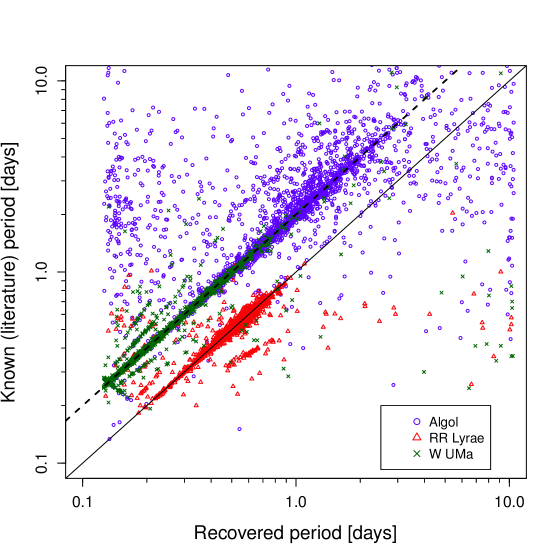
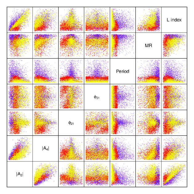
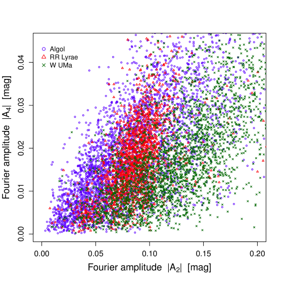
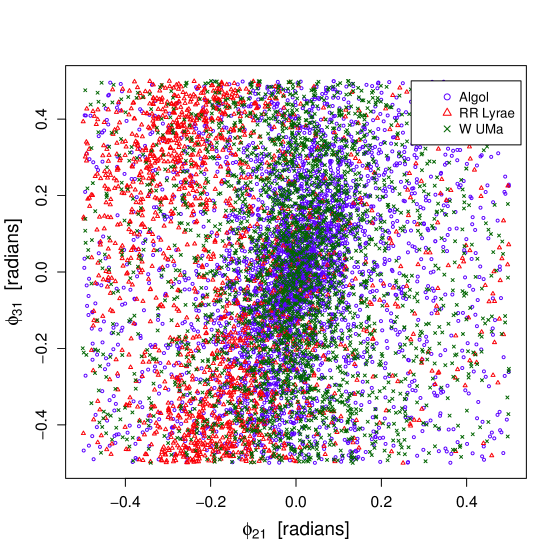
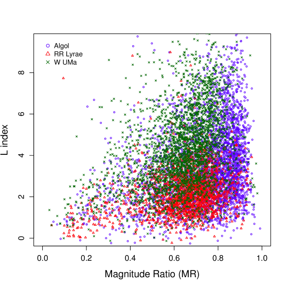
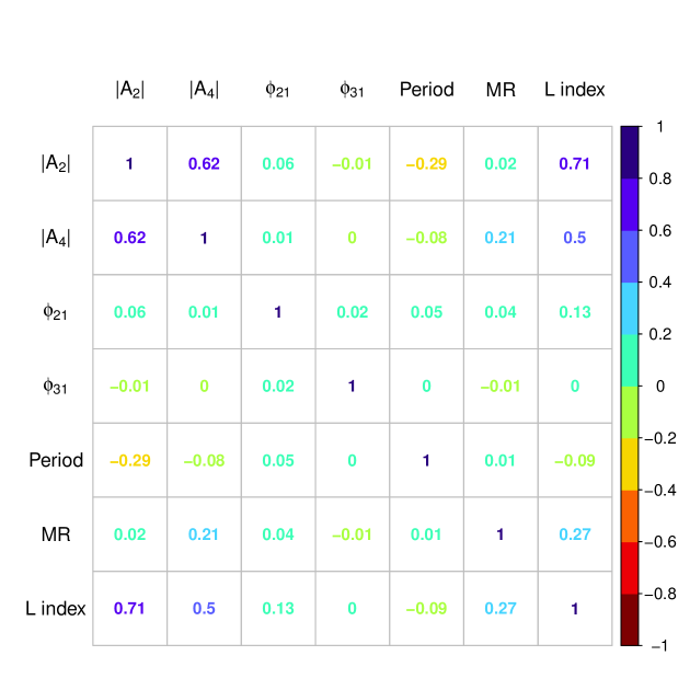
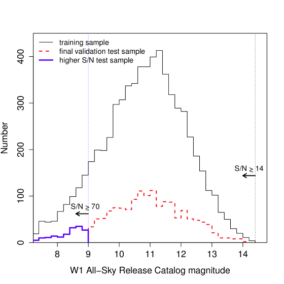
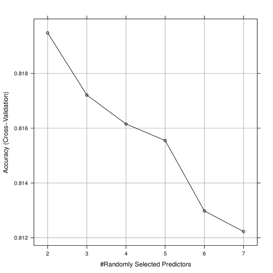
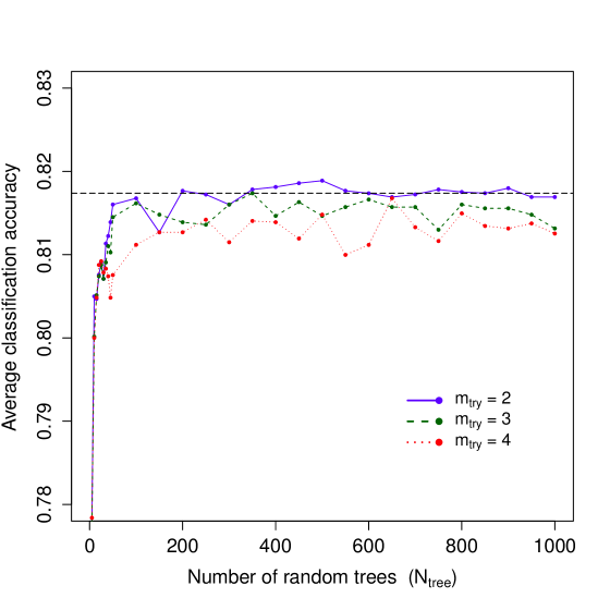
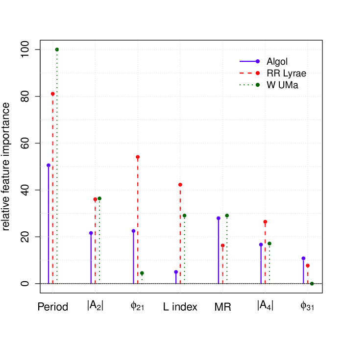
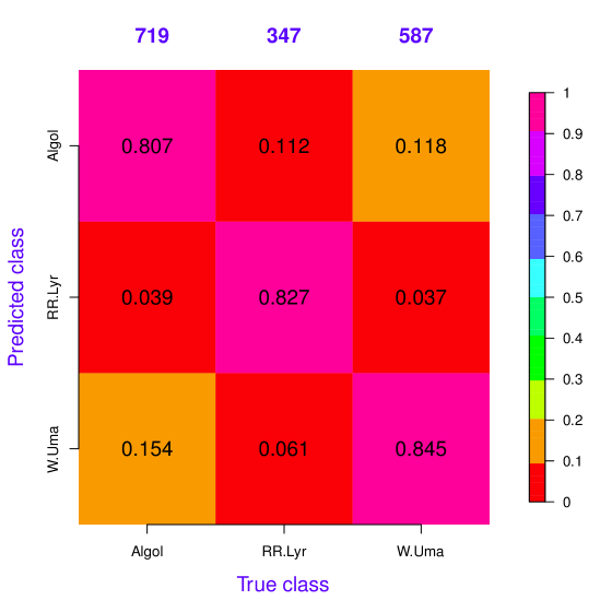
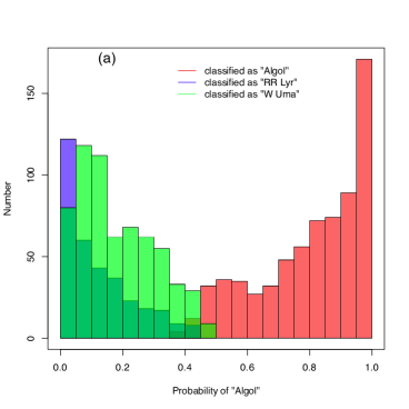
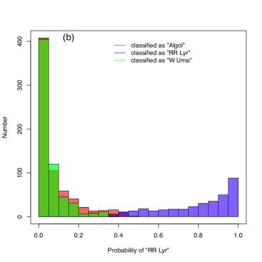
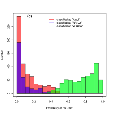
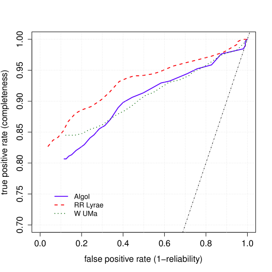

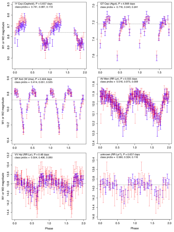
| Method | Med. Accuracy aaMedian and maximum achieved accuracies from a 10-fold cross-validation on the training sample. | Max. Accuracy aaMedian and maximum achieved accuracies from a 10-fold cross-validation on the training sample. | Training time bbAverage runtime to fit training model using parallel processing on a 12-core 2.4 GHz/core Macintosh with 60 GB of RAM. | Pred. time ccAverage runtime to predict classes and compute probabilities for 1653 feature vectors in our final validation test sample (Section 5.3). | p-value ddProbability value for H0: difference in mean accuracy relative to RF is zero. |
|---|---|---|---|---|---|
| (sec) | (sec) | (%) | |||
| NNET | 0.815 | 0.830 | 375.32 | 0.78 | 99.99 |
| NN | 0.728 | 0.772 | 6.42 | 0.55 | |
| RF | 0.819 | 0.840 | 86.75 | 0.77 | |
| SVM | 0.798 | 0.814 | 75.66 | 1.77 | 3.11 |