Mutual information of Contingency Tables and Related Inequalities

Peter Harremoës Copenhagen Business College
Copenhagen, Denmark
Email: harremoes@ieee.org
Abstract

For testing independence it is very popular to use either the χ2superscript𝜒2\chi^{2}-statistic or G2superscript𝐺2G^{2}-statistics (mutual information). Asymptotically both are χ2superscript𝜒2\chi^{2}-distributed so an obvious question is which of the two statistics that has a distribution that is closest to the χ2superscript𝜒2\chi^{2}-distribution. Surprisingly the distribution of mutual information is much better approximated by a χ2superscript𝜒2\chi^{2}-distribution than the χ2superscript𝜒2\chi^{2}-statistic. For technical reasons we shall focus on the simplest case with one degree of freedom. We introduce the signed log-likelihood and demonstrate that its distribution function can be related to the distribution function of a standard Gaussian by inequalities. For the hypergeometric distribution we formulate a general conjecture about how close the signed log-likelihood is to a standard Gaussian, and this conjecture gives much more accurate estimates of the tail probabilities of this type of distribution than previously published results. The conjecture has been proved numerically in all cases relevant for testing independence and further evidence of its validity is given.

I Choice of statistic

We consider the problem of testing independence in a discrete setting. Here we shall follow the classic approach to this problem as developed by Pearson, Neuman and Fisher. The question is whether a sample with observation counts (Xij)subscript𝑋𝑖𝑗\left(X_{ij}\right) has been generated by the distribution Q=(qij)𝑄subscript𝑞𝑖𝑗Q=\left(q_{ij}\right) where qij=sitjsubscript𝑞𝑖𝑗subscript𝑠𝑖subscript𝑡𝑗q_{ij}=s_{i}\cdot t_{j} for some probability vectors (si)subscript𝑠𝑖\left(s_{i}\right) and (tj)subscript𝑡𝑗\left(t_{j}\right) reflecting independence. We introduce the marginal counts Ri=jXijsubscript𝑅𝑖subscript𝑗subscript𝑋𝑖𝑗R_{i}=\sum_{j}X_{ij} and Sj=iXijsubscript𝑆𝑗subscript𝑖subscript𝑋𝑖𝑗S_{j}=\sum_{i}X_{ij} and the sample size N=ijXij𝑁subscript𝑖𝑗subscript𝑋𝑖𝑗N=\sum_{ij}X_{ij}. The maximum likelihood estimates of probability vectors (si)subscript𝑠𝑖\left(s_{i}\right) and (tj)subscript𝑡𝑗\left(t_{j}\right) are given by si=RiNsubscript𝑠𝑖subscript𝑅𝑖𝑁s_{i}=\frac{R_{i}}{N} and tj=SjNsubscript𝑡𝑗subscript𝑆𝑗𝑁t_{j}=\frac{S_{j}}{N} leading to qij=RiSjN2subscript𝑞𝑖𝑗subscript𝑅𝑖subscript𝑆𝑗superscript𝑁2q_{ij}=\frac{R_{i}\cdot S_{j}}{N^{2}}. We also introduce the empirical distribution P^=(XijN)^𝑃subscript𝑋𝑖𝑗𝑁\hat{P}=\left(\frac{X_{ij}}{N}\right) .

Often one uses one of the Csiszár [1] f𝑓f-divergences

Df(P^,Q)=i,jqijf(p^ijqij).subscript𝐷𝑓^𝑃𝑄subscript𝑖𝑗subscript𝑞𝑖𝑗𝑓subscript^𝑝𝑖𝑗subscript𝑞𝑖𝑗D_{f}\left(\hat{P},Q\right)={\textstyle\sum\limits_{i,j}}q_{ij}f\left(\frac{\hat{p}_{ij}}{q_{ij}}\right). (1)

The null hypothesis is accepted if the test statistic Df(P^,Q)subscript𝐷𝑓^𝑃𝑄D_{f}\left(\hat{P},Q\right) is small and rejected if Df(P^,Q)subscript𝐷𝑓^𝑃𝑄D_{f}\left(\hat{P},Q\right) is large. Whether Df(P^,Q)subscript𝐷𝑓^𝑃𝑄D_{f}\left(\hat{P},Q\right) is considered to be small or large depends on the significance level [2]. The most important cases are obtained for the convex functions f(t)=n(t1)2𝑓𝑡𝑛superscript𝑡12f(t)=n(t-1)^{2} and f(t)=2ntlnt𝑓𝑡2𝑛𝑡𝑡f(t)=2nt\ln t leading to the Pearson χ2superscript𝜒2\chi^{2}-statistic

χ2=i,j(XijNqij)2Nqnjsuperscript𝜒2subscript𝑖𝑗superscriptsubscript𝑋𝑖𝑗𝑁subscript𝑞𝑖𝑗2𝑁subscript𝑞𝑛𝑗\chi^{2}={\textstyle\sum\limits_{i,j}}\frac{(X_{ij}-Nq_{ij})^{2}}{Nq_{nj}} (2)

and the likelihood ratio statistic

G2=2i,jXijlnXijNqij.superscript𝐺22subscript𝑖𝑗subscript𝑋𝑖𝑗subscript𝑋𝑖𝑗𝑁subscript𝑞𝑖𝑗G^{2}=2{\textstyle\sum\limits_{i,j}}X_{ij}\ln\frac{X_{ij}}{Nq_{ij}}. (3)

We note that G2superscript𝐺2G^{2} equals the mutual information between the indices i𝑖i and j𝑗j times 2n2𝑛2n when the empirical distribution P^^𝑃\hat{P} is used as joint distribution over i𝑖i and j𝑗j. See [3] for a short introduction to contingency tables and further references on the subject.

One way of choosing between various statistics is by computing their asymptotic efficiency [4, 5] but for finite sample size such results are difficult to use. Therefore we will turn our attention to another property that is of importance in choosing a statistic.

20202040404060606080808010010010012012012014014014020202040404060606080808010010010012012012014014014000
Figure 1: Quantiles of twice mutual information vs. a χ2superscript𝜒2\chi^{2}-distribution.

For the practical use of a statistic it is important to calculate or estimate the distribution of the statistic. This can be done by exact calculation, by approximations and by simulations. Exact calculations may be both time consuming and difficult. Simulation often requires statistical insight and programming skills. Therefore most statistical tests use approximations to calculate the distribution of the statistic. The distribution of the χ2superscript𝜒2\chi^{2}-statistic becomes closer and closer to the χ2superscript𝜒2\chi^{2}-distributions as the sample size tends to infinity. For a large sample size the empirical distribution will with high probability be close to the generating distribution and any Csiszár f𝑓f-divergence Dfsubscript𝐷𝑓D_{f} can be approximated by a scaled version of the χ2superscript𝜒2\chi^{2}-statistic

Df(P,Q)f′′(0)2χ2(P,Q).subscript𝐷𝑓𝑃𝑄superscript𝑓′′02superscript𝜒2𝑃𝑄D_{f}\left(P,Q\right)\approx\frac{f^{\prime\prime}\left(0\right)}{2}\cdot\chi^{2}\left(P,Q\right).

Therefore the distribution of any f𝑓f-divergence may be approximated by a scaled χ2superscript𝜒2\chi^{2}-distribution, i.e. a Gamma distribution. From this argument one might get the impression that the distribution of the χ2superscript𝜒2\chi^{2}-statistic is closer to the χ2superscript𝜒2\chi^{2}-distribution. Figure 1 and Figure 2 show that this is far from the the case. Figure 1 shows that the distribution of theG2superscript𝐺2G^{2}-statistic (i.e. mutual information) is almost as close to a χ2superscript𝜒2\chi^{2}-distribution as it could be taking into account that mutual information has a discrete distribution. Each step is intersected very close to its mid point. Figure 2 shows that the distribution of the Pearson statistic (χ2superscript𝜒2\chi^{2}-statistic) is very different when the observed counts deviates from the expected distribution and the intersection property only holds when each cell in the contingency table contains at least 10 observations. These two plots show that at least in some cases the distribution of mutual information is much closer to a (scaled) χ2superscript𝜒2\chi^{2}-distribution than the Pearson χ2superscript𝜒2\chi^{2}-statistic is. The next question is whether there are situations where mutual information is not approximately χ2superscript𝜒2\chi^{2}-distributed. For contingency tables that are much less symmetric the intersection property of Figure 1 is not satisfied when the G𝐺G-statistic is plotted against the χ2superscript𝜒2\chi^{2}-distrbution so in the rest of this paper a different type of plots will be used.

20202040404060606080808010010010012012012014014014020202040404060606080808010010010012012012014014014000
Figure 2: Quantiles of the χ2superscript𝜒2\chi^{2}-statistic vs. a χ2superscript𝜒2\chi^{2}-distribution.

The use of the G2superscript𝐺2G^{2}-statistic rather than the χ2superscript𝜒2\chi^{2}-statistic has become more and more popular since this was recommended in the 1981 edition of the popular textbook of Sokal and Rohlf [6]. A summery of what the typical recommended about whether one should use the χ2superscript𝜒2\chi^{2}-statistic or the G2superscript𝐺2G^{2}-Statistic was given by T. Dunning [7]. The short version is that the statistic is approximately χ2superscript𝜒2\chi^{2}-distributed when each bin contains at least 5 observations or the calculated variance for each bin is at least 5, and if any bin contains more than twice the expected number observations then the G2superscript𝐺2G^{2}-statistic is preferable to the χ2superscript𝜒2\chi^{2}-statistic. If the test has only one degree of freedom one often recommend each bin contain at least 10 observations.

In this paper we will let τ𝜏\tau denote the circle constant 2π2𝜋2\pi and let ϕitalic-ϕ\phi denote the standard Gaussian density

exp(x22)τ1/2.superscript𝑥22superscript𝜏12\frac{\exp\left(-\frac{x^{2}}{2}\right)}{\tau^{\nicefrac{{1}}{{2}}}}.

We let ΦΦ\Phi denote the distribution function of the standard Gaussian

Φ(t)=tϕ(x)dx.Φ𝑡superscriptsubscript𝑡italic-ϕ𝑥d𝑥\Phi\left(t\right)=\int_{-\infty}^{t}\phi\left(x\right)\,\text{d}x~{}.

The rest of the paper is organized as follows. In Section II we formulate a general inequality for point probabilities in general contingency tables in terms of mutual information. In Section III we intrroduce special notation for 2×2222\times 2 contingency tables, and we introduce the signed log-likelihood of a 2×2222\times 2 contingency table. In Section IV we introduce the signed log-likelihood for exponential families. In Section V we formulate some sharp inequalities for waiting times and as corollaries we obtain intersection inequalies for binomial distributions and Poisson distributions. In Section VI we explain how the intersection property has been checked numerically for all cases relevant for testing independence. We end with a short discussion. Most of the proofs, detailed descriptions of the numerical algorithms, and further plots are given in an appendix. The appendix also contains some material on larger contingency tables. The appendix can be found in the arXiv-version of this paper.

II Contingency tables

We consider a contingeny table

Total
X11subscript𝑋11X_{11} X12subscript𝑋12X_{12} \cdots X1subscript𝑋1X_{1\text{$\ell$}} R1subscript𝑅1R_{1}
X21subscript𝑋21X_{21} X22subscript𝑋22X_{22} \cdots X2subscript𝑋2X_{2\ell} R2subscript𝑅2R_{2}
\vdots \vdots \ddots \vdots \vdots
Xk1subscript𝑋𝑘1X_{k1} Xk2subscript𝑋𝑘2X_{k2} \cdots Xksubscript𝑋𝑘X_{k\ell} Rksubscript𝑅𝑘R_{k}
Total S1subscript𝑆1S_{1} S2subscript𝑆2S_{2} \cdots Ssubscript𝑆S_{\text{$\ell$}} N𝑁N

We fix the row counts Risubscript𝑅𝑖R_{i} and the coloum counts Sjsubscript𝑆𝑗S_{j} and we are interseted in the distribution of the counts Xijsubscript𝑋𝑖𝑗X_{ij} under the null hypothesis that the counted features are independent. These probabilities are given by

Pr(Xij=xij)Prsubscript𝑋𝑖𝑗subscript𝑥𝑖𝑗\displaystyle\Pr\left(X_{ij}=x_{ij}\right) =(Nxij)(NRi)(NSj)absent𝑁subscript𝑥𝑖𝑗𝑁subscript𝑅𝑖𝑁subscript𝑆𝑗\displaystyle=\frac{\left(\begin{array}[]{c}N\\ x_{ij}\end{array}\right)}{\left(\begin{array}[]{c}N\\ R_{i}\end{array}\right)\left(\begin{array}[]{c}N\\ S_{j}\end{array}\right)}
=iRi!,jSj!N!i,jxij!.\displaystyle=\frac{\prod_{i}R_{i}!\prod_{,j}S_{j}!}{N!\prod_{i,j}x_{ij}!}\,.

The (empirical) mutual information I𝐼I of the contingency table is calculated as

NI𝑁𝐼\displaystyle N\cdot I =ND(P^Q)=i,jXijlnxijNqij=i,jXijlnNxijRiSjabsent𝑁𝐷conditional^𝑃𝑄subscript𝑖𝑗subscript𝑋𝑖𝑗subscript𝑥𝑖𝑗𝑁subscript𝑞𝑖𝑗subscript𝑖𝑗subscript𝑋𝑖𝑗𝑁subscript𝑥𝑖𝑗subscript𝑅𝑖subscript𝑆𝑗\displaystyle=N\cdot D\left(\left.\hat{P}\right\|Q\right)={\textstyle\sum\limits_{i,j}}X_{ij}\ln\frac{x_{ij}}{Nq_{ij}}={\textstyle\sum\limits_{i,j}}X_{ij}\ln\frac{N\cdot x_{ij}}{R_{i}\cdot S_{j}}
=i,jxijln(xij)iRiln(Ri)jSjln(Sj)absentsubscript𝑖𝑗subscript𝑥𝑖𝑗subscript𝑥𝑖𝑗subscript𝑖subscript𝑅𝑖subscript𝑅𝑖subscript𝑗subscript𝑆𝑗subscript𝑆𝑗\displaystyle=\sum_{i,j}x_{ij}\ln\left(x_{ij}\right)-\sum_{i}R_{i}\ln\left(R_{i}\right)-\sum_{j}S_{j}\ln\left(S_{j}\right)
+Nln(N).𝑁𝑁\displaystyle\,\,+N\ln\left(N\right).
Theorem 1.

For a contingency table without empty cells the following inequality holds

Pr(Xij=xij)eNI(iRi,jSjτ(k1)(1)Ni,jxij)1/2.\Pr\left(X_{ij}=x_{ij}\right)\leq\mathrm{e}^{{}^{-N\cdot I}}\left(\frac{\prod_{i}R_{i}\prod_{,j}S_{j}}{\tau^{\left(k-1\right)\left(\ell-1\right)}N\prod_{i,j}x_{ij}}\right)^{\nicefrac{{1}}{{2}}}. (4)

Although Inequality 4 is quite tigth for most values of x𝑥x it cannot be used to provide bounds on the tail probabilities because it is not valid when one of the cells is empty. Inequalities

Pr(Xij=xij)CeNI(iRi,jSjτ(k1)(1)Ni,jxij)1/2\Pr\left(X_{ij}=x_{ij}\right)\geq C\mathrm{e}^{{}^{-N\cdot I}}\left(\frac{\prod_{i}R_{i}\prod_{,j}S_{j}}{\tau^{\left(k-1\right)\left(\ell-1\right)}N\prod_{i,j}x_{ij}}\right)^{\nicefrac{{1}}{{2}}}

where C<1𝐶1C<1 is a positive constant can also be proved, but the optimal constant will depend on the sample size and on the size of the contingency table.

III Contingency tables with one degree of freedom

In this paper our theoretical results will focus on contingency tables with one degree of freedom and there are several reasons for this. The distribution of the statistic is closely related to the hypergeometric distribution that is well studied in the literature. It is know that the use of the χ2superscript𝜒2\chi^{2}-distributions is most problematic when the number of degrees of freedom is small. Results of testing independency can be compared with similar results for testing goodness of fit that are only available for one degree of freedom.

First we will introduce some special notation. We consider a contingency table

Total
X𝑋X rX𝑟𝑋r-X r𝑟r
nX𝑛𝑋n-X Nr+X𝑁𝑟𝑋N-r+X Nr𝑁𝑟N-r
Total n𝑛n Nn𝑁𝑛N-n N𝑁N

If the marginal counts are kept fixed and independence is assumed then the distribution of X𝑋X is a hypergeometric distribution with parameters (N,r,n)𝑁𝑟𝑛\left(N,r,n\right) and point probabilities

P(X=x)=(rx)(Nrnx)(Nn)𝑃𝑋𝑥𝑟𝑥𝑁𝑟𝑛𝑥𝑁𝑛P\left(X=x\right)=\frac{\left(\begin{array}[]{c}r\\ x\end{array}\right)\left(\begin{array}[]{c}N-r\\ n-x\end{array}\right)}{\left(\begin{array}[]{c}N\\ n\end{array}\right)}

This hypergeometric disribution has mean value nrN𝑛𝑟𝑁\frac{nr}{N} and variance nr(Nr)(Nn)N2(N1)𝑛𝑟𝑁𝑟𝑁𝑛superscript𝑁2𝑁1\frac{nr\left(N-r\right)\left(N-n\right)}{N^{2}\left(N-1\right)}. For 2×2222\times 2 contingency tables we introduce a random variable G𝐺G that is related to mutual information in the same way as χ𝜒\chi is related to χ2superscript𝜒2\chi^{2}.

Definition 2.

The signed log-likelihood of a 2×2222\times 2 contingency table is defined as

G(X)={(2NI(X))1/2,for X<nrN;+(2NI(X))1/2,for XnrN.𝐺𝑋casessuperscript2𝑁𝐼𝑋12for 𝑋𝑛𝑟𝑁superscript2𝑁𝐼𝑋12for 𝑋𝑛𝑟𝑁G\left(X\right)=\left\{\begin{array}[]{cc}-\left(2N\cdot I\left(X\right)\right)^{\nicefrac{{1}}{{2}}},&\text{for }X<\frac{nr}{N};\\ +\left(2N\cdot I\left(X\right)\right)^{\nicefrac{{1}}{{2}}},&\text{for }X\geq\frac{nr}{N}.\end{array}\right.

With this notation the first factor in Inequality 4 can be written as eNIτ1/2=ϕ(G(x)).superscripte𝑁𝐼superscript𝜏12italic-ϕ𝐺𝑥\frac{\mathrm{e}^{{}^{-N\cdot I}}}{\tau^{\nicefrac{{1}}{{2}}}}=\phi\left(G\left(x\right)\right). A QQ-plot of G(X)𝐺𝑋G\left(X\right) against a standard Gaussian is given in Figure 3. This plot and other similar plots support the following intersection conjecture for hypergeometric distributions.

Conjecture 3.

For a 2×2222\times 2 contingency table let G(X)𝐺𝑋G\left(X\right) denote the signed log-likelihod. Then the quantile transform between G(X)𝐺𝑋G\left(X\right) and a standard Gaussian Z𝑍Z is a step function and the identity function intersects each step, i.e. Pr(X<x)<Pr(Zg(x))<Pr(Xx)Pr𝑋𝑥Pr𝑍𝑔𝑥Pr𝑋𝑥\Pr\left(X<x\right)<\Pr\left(Z\leq g\left(x\right)\right)<\Pr\left(X\leq x\right) for all integers x.𝑥x.

If n𝑛n is much smaller than N𝑁N then the distribution of X𝑋X can be approximated by binomial distribution bin(n,p)𝑏𝑖𝑛𝑛𝑝bin\left(n,p\right) where p=r/N𝑝𝑟𝑁p=\nicefrac{{r}}{{N}}. If n𝑛n is much smaller than N𝑁N we can approximate the mutual information by the information divergence xnlnx/np+(1xn)ln(1x/n1p).𝑥𝑛𝑥𝑛𝑝1𝑥𝑛1𝑥𝑛1𝑝\frac{x}{n}\ln\frac{\nicefrac{{x}}{{n}}}{p}+\left(1-\frac{x}{n}\right)\ln\left(\frac{1-\nicefrac{{x}}{{n}}}{1-p}\right). Therefore it is of interest to see if the intersection conjecture holds in the limiting case of a binomial distribution.

44-422-222244466688844-422-222244466688800
Figure 3: Quantiles of g(X)𝑔𝑋g\left(X\right) against a standard Gaussian when X𝑋X is hypergeometric with parameters N=40,𝑁40N=40, n=15𝑛15n=15, and r=15.𝑟15r=15. The streight line corresponds to a perfect match with a Gaussian distribution.

IV The signed log-likelihood for exponential families

Consider the 1-dimensional exponential family Pβsubscript𝑃𝛽P_{\beta} where

dPβdP0(x)=exp(βx)Z(β)dsubscript𝑃𝛽dsubscript𝑃0𝑥𝛽𝑥𝑍𝛽\frac{\text{d}P_{\beta}}{\text{d}P_{0}}\left(x\right)=\frac{\exp\left(\beta\cdot x\right)}{Z\left(\beta\right)}

and Z𝑍Z denotes the moment generating function given by Z(β)=exp(βx)dP0x.𝛽𝛽𝑥dsubscript𝑃0𝑥\left(\beta\right)=\int\exp\left(\beta\cdot x\right)\,\text{d}P_{0}x. Let Pμsuperscript𝑃𝜇P^{\mu} denote the element in the exponential family with mean value μ,𝜇\mu, and let β^(μ)^𝛽𝜇\hat{\beta}\left(\mu\right) denote the corresponding maximum likelihood estimate of β.𝛽\beta. Let μ0subscript𝜇0\mu_{0} denote the mean value of P0.subscript𝑃0P_{0}. Then

D(PμP0)𝐷conditionalsuperscript𝑃𝜇subscript𝑃0\displaystyle D\left(P^{\mu}\|P_{0}\right) =ln(dPμdP0(x))dPμx.absentdsuperscript𝑃𝜇dsubscript𝑃0𝑥dsuperscript𝑃𝜇𝑥\displaystyle=\int\ln\left(\frac{\text{d}P^{\mu}}{\text{d}P_{0}}\left(x\right)\right)\,\text{d}P^{\mu}x.
=μβ^(μ)ln(Z(β^(μ)))absent𝜇^𝛽𝜇𝑍^𝛽𝜇\displaystyle=\mu\cdot\hat{\beta}\left(\mu\right)-\ln\left(Z\left(\hat{\beta}\left(\mu\right)\right)\right)
Definition 4.

Let X𝑋X be a random variable with distribution P0.subscript𝑃0P_{0}. Then the G𝐺G-transform g(X)𝑔𝑋g\left(X\right) of X𝑋X is the random variable given by

G(x)={(2D(PxP0))1/2,for x<μ0;+(2D(PxP0))1/2,for xμ0.𝐺𝑥casessuperscript2𝐷conditionalsuperscript𝑃𝑥subscript𝑃012for 𝑥subscript𝜇0superscript2𝐷conditionalsuperscript𝑃𝑥subscript𝑃012for 𝑥subscript𝜇0G\left(x\right)=\left\{\begin{array}[]{cc}-\left(2D\left(P^{x}\|P_{0}\right)\right)^{\nicefrac{{1}}{{2}}},&\text{for }x<\mu_{0};\\ +\left(2D\left(P^{x}\|P_{0}\right)\right)^{\nicefrac{{1}}{{2}}},&\text{for }x\geq\mu_{0}.\end{array}\right.
Theorem 5.

Let X𝑋X denote a binomial distributed or Poisson distributed random variable and let G(X)𝐺𝑋G\left(X\right) denote the G𝐺G-transform of X.𝑋X. The quantile transform between g(X)𝑔𝑋g\left(X\right) and a standard Gaussian Z𝑍Z is a step function and the identity function intersects each step, i.e. P(X<k)<P(Zg(k))<P(Xk)𝑃𝑋𝑘𝑃𝑍𝑔𝑘𝑃𝑋𝑘P\left(X<k\right)<P\left(Z\leq g\left(k\right)\right)<P\left(X\leq k\right) for all integers k.𝑘k.

For Poisson distributions this result was proved in [4] where the result for binomial distributions was also conjectured. A proof of this conjecture was recently given by Serov and Zubkov [8]. Were we will prove that the intersection results for binomial distributions and Poisson distributions follows from more general results for waiting times. We will need the following general lemma.

Lemma 6.

In an exponential family with G=±(2D(PμPμ0))1/2𝐺plus-or-minussuperscript2𝐷conditionalsuperscript𝑃𝜇superscript𝑃subscript𝜇012G=\pm\left(2D\left(\left.P^{\mu}\right\|P^{\mu_{0}}\right)\right)^{\nicefrac{{1}}{{2}}} one has

μ0Φ(G)=ϕ(G)V(μ0)μ0μG.subscript𝜇0Φ𝐺italic-ϕ𝐺𝑉subscript𝜇0subscript𝜇0𝜇𝐺\frac{\partial}{\partial\mu_{0}}\Phi\left(G\right)=\frac{\phi\left(G\right)}{V\left(\mu_{0}\right)}\cdot\frac{\mu_{0}-\mu}{G}.

V Inequalities for waiting times

Next we will formulate some inequalities for waiting times. Let nb(p,)𝑛𝑏𝑝nb\left(p,\ell\right) denote distribution of the number of failures before the \ell’th succes in a Bernoulli process with success probability p.𝑝p. The mean value is given by μ=1pp𝜇1𝑝𝑝\mu=\ell\frac{1-p}{p}.

Lemma 7.

If the distribution if W1subscript𝑊1W_{1} is nb(p,)𝑛𝑏𝑝nb\left(p,\ell\right) with μ=1pp𝜇1𝑝𝑝\mu=\ell\frac{1-p}{p} then the partial derivative of the point probaiblity equals

μPr(W1=k)=Pr(W2=k1)Pr(W2=k).𝜇Prsubscript𝑊1𝑘Prsubscript𝑊2𝑘1Prsubscript𝑊2𝑘\frac{\partial}{\partial\mu}\Pr\left(W_{1}=k\right)=\Pr\left(W_{2}=k-1\right)-\Pr\left(W_{2}=k\right).

where W2subscript𝑊2W_{2} is nb(p,+1).𝑛𝑏𝑝1nb\left(p,\ell+1\right).

Theorem 8.

For any [1;[1\ell\in\left[1;\infty\right[ the random variable W2subscript𝑊2W_{2} with distribution Nb(p,)𝑁𝑏𝑝Nb\left(p,\ell\right)satisfies

Φ(Gnb(p,)(k))Pr(W2k),Φsubscript𝐺𝑛𝑏𝑝𝑘Prsubscript𝑊2𝑘\Phi\left(G_{nb\left(p,\ell\right)}\left(k\right)\right)\leq\Pr\left(W_{2}\leq k\right),

where Gnb(p,)denotessubscript𝐺𝑛𝑏𝑝𝑑𝑒𝑛𝑜𝑡𝑒𝑠G_{nb\left(p,\ell\right)denotes} the signed log-likelihood of the negative binomial distribution.

Proof:

For any k,l𝑘𝑙k,l one has to prove that Pr(W2k)Φ(Gnb(p,)(k))Prsubscript𝑊2𝑘Φsubscript𝐺𝑛𝑏𝑝𝑘\Pr\left(W_{2}\leq k\right)-\Phi\left(G_{nb\left(p,\ell\right)}\left(k\right)\right) is non-negative. If p=0𝑝0p=0 or p=1𝑝1p=1 this is obvious. The result is obtained by differentiating several times with respect to the mean value. See Appendix for details. ∎

A Gamma distribution can be considered as a limit of negative binomial distributions, which leads to the following corollary.

Corollary 9.

If W𝑊W denotes a Gamma distribution then

Φ(GΓ(x))Pr(Wx).Φsubscript𝐺Γ𝑥Pr𝑊𝑥\Phi\left(G_{\Gamma}\left(x\right)\right)\leq\Pr\left(W\leq x\right).

A similar inequality is satisfied by inverse Gaussian distributions that are waiting times for browning motions.

Theorem 10.

For any x[0;[𝑥0x\in\left[0;\infty\right[ the random variable W𝑊W with distribution IG(μ,λ)𝐼𝐺𝜇𝜆IG\left(\mu,\lambda\right) satisfies

Φ(GIG(μ,λ)(k))Pr(Wk),Φsubscript𝐺𝐼𝐺𝜇𝜆𝑘Pr𝑊𝑘\Phi\left(G_{IG\left(\mu,\lambda\right)}\left(k\right)\right)\leq\Pr\left(W\leq k\right),

where GIG(μ,λ)subscript𝐺𝐼𝐺𝜇𝜆G_{IG\left(\mu,\lambda\right)} denotes the signed log-likelihood of the inverse Gaussian.

Proof:

The proof uses the same technique as in [4]. See Appendix. ∎

Assume that M𝑀M is binomial bin(n,p)𝑏𝑖𝑛𝑛𝑝bin\left(n,p\right) and W𝑊W is negative binomial nb(p,).𝑛𝑏𝑝nb\left(p,\ell\right). Then

Pr(M)=Pr(W+n).Pr𝑀Pr𝑊𝑛\Pr\left(M\geq\ell\right)=\Pr\left(W+\ell\leq n\right).

The divergence can be calcuated as

D(nb(p1,)nb(p2))=p1(p1lnp1p2+(1p1)ln1p11p2).𝐷conditional𝑛𝑏subscript𝑝1𝑛𝑏subscript𝑝2subscript𝑝1subscript𝑝1subscript𝑝1subscript𝑝21subscript𝑝11subscript𝑝11subscript𝑝2D\left(\left.nb\left(p_{1},\ell\right)\right\|nb\left(p_{2}\ell\right)\right)=\\ \frac{\ell}{p_{1}}\left(p_{1}\ln\frac{p_{1}}{p_{2}}+\left(1-p_{1}\right)\ln\frac{1-p_{1}}{1-p_{2}}\right).

If p1=nsubscript𝑝1𝑛\frac{\ell}{p_{1}}=n then

D(nb(p1,)nb(p2))=n(p1lnp1p2+(1p1)ln1p11p2)=D(bin(n,n)bin(n,p)).𝐷conditional𝑛𝑏subscript𝑝1𝑛𝑏subscript𝑝2𝑛subscript𝑝1subscript𝑝1subscript𝑝21subscript𝑝11subscript𝑝11subscript𝑝2𝐷conditional𝑏𝑖𝑛𝑛𝑛𝑏𝑖𝑛𝑛𝑝D\left(\left.nb\left(p_{1},\ell\right)\right\|nb\left(p_{2}\ell\right)\right)\\ =n\left(p_{1}\ln\frac{p_{1}}{p_{2}}+\left(1-p_{1}\right)\ln\frac{1-p_{1}}{1-p_{2}}\right)\\ =D\left(\left.bin\left(n,\frac{\ell}{n}\right)\right\|bin\left(n,p\right)\right).

If Gbinsubscript𝐺𝑏𝑖𝑛G_{bin} is the signed likelihood log-likelihood of bin(n,p)𝑏𝑖𝑛𝑛𝑝bin\left(n,p\right) and Gnbsubscript𝐺𝑛𝑏G_{nb}is the signed log-likelihood of nb(p,)𝑛𝑏𝑝nb\left(p,\ell\right) then Gbin()=Gnb(n).subscript𝐺𝑏𝑖𝑛subscript𝐺𝑛𝑏𝑛G_{bin}\left(\ell\right)=-G_{nb}\left(n\right). This shows that if the log-likelihood of a the negative binomial distributions are close to Gaussian then the same is true for the signed log-likelihood of binomial distribtions. Our inequality for the negative binomial distribution can be translated into an inequality for the binomial distribution.

Theorem 11.

Binomial distributions satisfy the intersection property.

Proof:

We have to prove that

Pr(Sn<)Φ(Gbin(n,p)())Pr(Sn).Prsubscript𝑆𝑛Φsubscript𝐺𝑏𝑖𝑛𝑛𝑝Prsubscript𝑆𝑛\Pr\left(S_{n}<\ell\right)\leq\Phi\left(G_{bin\left(n,p\right)}\left(\ell\right)\right)\leq\Pr\left(S_{n}\leq\ell\right).

We will only prove the left inequality since the right inequality follows from the left inequality by replacing p𝑝p by 1p1𝑝1-p and replacing \ell by n.𝑛n-\ell. We have

Pr(Sn<)Prsubscript𝑆𝑛\displaystyle\Pr\left(S_{n}<\ell\right) =\displaystyle= 1Pr(Sn)=1Pr(W1n)1Prsubscript𝑆𝑛1Prsubscript𝑊1𝑛\displaystyle 1-\Pr\left(S_{n}\geq\ell\right)=1-\Pr\left(W_{1}\leq n\right)
\displaystyle\leq 1Φ(Gnb(p,)(n))=Φ(Gnb(p,)(n))1Φsubscript𝐺𝑛𝑏𝑝𝑛Φsubscript𝐺𝑛𝑏𝑝𝑛\displaystyle 1-\Phi\left(G_{nb\left(p,\ell\right)}\left(n\right)\right)=\Phi\left(-G_{nb\left(p,\ell\right)}\left(n\right)\right)
=\displaystyle= Φ(Gbin(n,p)()).Φsubscript𝐺𝑏𝑖𝑛𝑛𝑝\displaystyle\Phi\left(G_{bin\left(n,p\right)}\left(\ell\right)\right).

Note that Theorem 8 cannot be proved from Theorem 11 because the number parameter for a binomial distribution has to be an integer while the number parameter of a negative binomial distribution may assume any positive value.Since a Poisson distribution is a limit of binomial distributions we get the following corollary.∎

Corollary 12.

Poisson distributions have the intersection property.

These results allow us to sharpen a bound for the tail probabilities of a hypergeometric distribution proved by Chvátal [9].

Corollary 13.

Let the distribution of X𝑋X be hypergeometric with parameters (N,n,r)𝑁𝑛𝑟\left(N,n,r\right) and assume that xnr/N.𝑥𝑛𝑟𝑁x\leq nr/N. Then

Pr(X<)<Φ((2nD((xn,1xn)(rN,1rN)))).Pr𝑋Φ2𝑛𝐷conditional𝑥𝑛1𝑥𝑛𝑟𝑁1𝑟𝑁\Pr\left(X<\ell\right)<\Phi\left(-\left(2nD\left(\left.\left(\frac{x}{n},1-\frac{x}{n}\right)\right\|\left(\frac{r}{N},1-\frac{r}{N}\right)\right)\right)\right). (5)

If we assume that mutual information has (scaled) χ2superscript𝜒2\chi^{{}^{2}}-distribution then we get an estimate of Pr(X<)Pr𝑋\Pr\left(X<\ell\right) that is less than Φ((2nD((xn,1xn)(rN,1rN))))Φ2𝑛𝐷conditional𝑥𝑛1𝑥𝑛𝑟𝑁1𝑟𝑁\Phi\left(-\left(2nD\left(\left.\left(\frac{x}{n},1-\frac{x}{n}\right)\right\|\left(\frac{r}{N},1-\frac{r}{N}\right)\right)\right)\right) but if we assume that the χ2superscript𝜒2\chi^{2}-statistic is χ2superscript𝜒2\chi^{2}-distributed we often get an estimate of Pr(X<)Pr𝑋\Pr\left(X<\ell\right) that violates Inequality 5 and in this sense mutual information has a distribution that is closer to the χ2superscript𝜒2\chi^{2}-distribution than the distribution of the χ2superscript𝜒2\chi^{2}-statistic is.

VI Numerical results

We have not yet been able to prove the intersection conjecture 3 for all hypergeometric distributions, but we have numerical calculations that confirm the conjecture for all cases that are relevant for testing independence.

Due to a symmetry of the problem we only have to check that Pr(X<x)<Pr(Zg(x))Pr𝑋𝑥Pr𝑍𝑔𝑥\Pr\left(X<x\right)<\Pr\left(Z\leq g\left(x\right)\right) holds for all 2×2222\times 2 contingency tables. For any finite sample size there are only finitely many contingency table with this sample size, so for any fixed sample size the inequality can be checked numerically. We have checked the hypergeometric intersection conjecture for any sample size up to 200.

If all bins contain at least 10 observations then the rule of thumb states that the χ2superscript𝜒2\chi^{2}-statistic and the G2superscript𝐺2G^{2}-statistic will both follow a χ2superscript𝜒2\chi^{2}-distribution, so it should be sufficient to test the hypothesis for x<10.𝑥10x<10.

As a rule of thumb the approximation by a binomial distribution is applicable when n0.1N𝑛0.1𝑁n\leq 0.1\cdot N and the intersection property holds for binomial distributions. Therefore we are only interested in the cases where n>0.1N𝑛0.1𝑁n>0.1\cdot N. By symmetry in the parameters it is also possible to approximate the distribution of X𝑋X by the binomial distribution bin(r,n/N)𝑏𝑖𝑛𝑟𝑛𝑁bin\left(r,\nicefrac{{n}}{{N}}\right) if r0.1N𝑟0.1𝑁r\leq 0.1\cdot N.

For testing independence one will normally choose a significance level α[0.001,0.1]𝛼0.0010.1\alpha\in\left[0.001,0.1\right]. If the p𝑝p-value can easily be bounded away from this interval there is no need to make a refined estimate of the p𝑝p-value via the intersection conjecture for the hypergeometric distribution. For x9𝑥9x\leq 9 the probability Pr(Xx)Pr𝑋𝑥\Pr\left(X\leq x\right) is bounded by Pr(X9).Pr𝑋9\Pr\left(X\leq 9\right). Let λ𝜆\lambda denote the mean of X𝑋X. Then Pr(X9)Pr(T9)Pr𝑋9Pr𝑇9\Pr\left(X\leq 9\right)\leq\Pr\left(T\leq 9\right) where T𝑇T is Poisson distributed with mean λ𝜆\lambda. Now Pr(T9)0.000974Pr𝑇90.000974\Pr\left(T\leq 9\right)\leq 0.000974 which is less that a significance level of 0.001 for λ22.7𝜆22.7\lambda\geq 22.7 so we are most interested in the cases where λ22.7𝜆22.7\lambda\leq 22.7. If we combine this with the condition n0.1N𝑛0.1𝑁n\geq 0.1\cdot N and r0.1N𝑟0.1𝑁r\geq 0.1\cdot N and that the mean of X𝑋X is nrN𝑛𝑟𝑁\frac{nr}{N} we see that we only have to check cases where N10022.7=2270𝑁10022.72270N\leq 100\cdot 22.7=2270. If we impose all these conditions we are left with a high but finite number of cases that can be checked numerically one by one. Further details are given in the appendix. The result is that the intersection conjecture holds for hypergeometric distributions for all cases that are of interest in relation to testing independence.

VII Discussion

The distribution of the signed log-likelihood is close a standard Gaussian for a variety of distributions. As an asymptotic result for large sample sizes this is not new [10], but for the most important distributions like the binomial distributions, the Poisson distributions, the negative binomial distributions, the inverse Gaussian distributions and the Gamma distributions we can formulate sharp inequalities that hold for any sample size. All these distributions have variance functions that are polynomials of order 2 and 3. Natural exponential families with polynomial variance functions of order at most 3 have been classified [11, 12] and there is a chance that one can formulate and prove a sharp inequality for each of these exponential families.

As we have seen there is strong numerical evidence that an intersection conjecture holds for all hypergeometric distributions, but a proof will be more difficult because the hypergeometric distributions do not form an exponential family and no variance function is available. In order to prove the conjecture it may prove useful to note that any hypergeometric distribution is a Poisson binomial distribution [13], i.e. the distribution of a sum of independent Bernoulli random variables with different success probabilities. Exploration of intersection conjectures for Poisson binomial distributions is work in progress and seems to be the most promising method direction in order to verify the intersection conjecture for the hypergeometric distributions.

VIII Acknowledgment

The author want to thank Gabor Tusnády, Lászlo Györfi, Joram Gat, Janós Komlos, and A. Zubkov for useful discussions.

References

  • [1] I. Csiszár, “Eine informationstheoretische Ungleichung und ihre Anwendung auf den Beweis der ergodizität von Markoffschen Ketten,” Publ. Math. Inst. Hungar. Acad., vol. 8, pp. 95–108, 1963.
  • [2] E. Lehman and G. Castella, Testing Statistical Hypotheses. New York: Springer, 3rd ed. ed., 2005.
  • [3] I. Csiszár and P. Shields, Information Theory and Statistics: A Tutorial. Foundations and Trends in Communications and Information Theory, Now Publishers Inc., 2004.
  • [4] P. Harremoës and G. Tusnády, “Information divergence is more χ2superscript𝜒2\chi^{2}-distributed than the χ2superscript𝜒2\chi^{2}-statistic,” in 2012 IEEE International Symposium on Information Theory (ISIT’2012), (Cambridge, Massachusetts, USA), pp. 538–543, IEEE, July 2012.
  • [5] P. Harremoës and I. Vajda, “On the Bahadur-efficient testing of uniformity by means of the entropy,” IEEE Trans. Inform Theory, vol. 54, pp. 321–331, Jan. 2008.
  • [6] R. R. Sokal and R. J. Rohlf, Biometry: the principles and practice of statistics in biological research. New York: Freeman, 1981. ISBN 0-7167-2411-1.
  • [7] T. Dunning, “Accurate methods for the statistics of surprise and coincidence,” Computational Linguistics, vol. 19, pp. 61–74, March 1993.
  • [8] A. M. Zubkov and A. A. Serov, “A complete proof of universal inequalities for the distribution function of the binomial law,” Theory Probab. Appl., vol. 57, pp. 539–544, Sept. 2013.
  • [9] V. Chvátal, “The tail of the hypergeometric distribution,” Discrete Mathematics, vol. 25, pp. 285–287, 1979.
  • [10] T. Zhang, “Limiting distribution of the G statistics,” Statistics and Probability Letters, vol. 78, pp. 1656–1661, 2008.
  • [11] C. Morris, “Natural exponential families with quadratic variance functions,” Ann. Statist., vol. 10, pp. 65–80, 1982.
  • [12] G. Letac and M. Mora, “Natural real exponential families with cubic variance functions,” Ann. Stat., vol. 18, no. 1, pp. 1–37, 1990.
  • [13] A. D. Barbour, L. Holst, and S. Janson, Poisson Approximation. Oxford Studies in Probability 2, Oxford: Clarendon Press, 1992.
  • [14] L. Györfi, P. Harremoës, and G. Tusnády, “Gaussian approximation of large deviation probabilities.” 2012.
  • [15] P. Harremoës, “Testing goodness-of-fit via rate distortion,” in Information Theory Workshop, Volos, Greece, 2009, pp. 17–21, IEEE, 2009.

This appendix contain proofs and further material that supports the conclusion of the paper.

Proof of Theorem 1

For the proof of our next theorem we need the following lemma.

Lemma 14.

The function i=1n(1+1xi)superscriptsubscriptproduct𝑖1𝑛11subscript𝑥𝑖\prod_{i=1}^{n}\left(1+\frac{1}{x_{i}}\right) is minimal under the constraint i=1nxi=λsuperscriptsubscript𝑖1𝑛subscript𝑥𝑖𝜆\sum_{i=1}^{n}x_{i}=\lambda and xi>0subscript𝑥𝑖0x_{i}>0 all xisubscript𝑥𝑖x_{i} are equal.

Proof:

We use the method of Lagrange multipliers. The matrix of partial derivatives is

(1x12i=1n(1+1xi)1+1x11x22i=1n(1+1xi)1+1x21xn2i=1n(1+1xi)1+1xn111).1superscriptsubscript𝑥12superscriptsubscriptproduct𝑖1𝑛11subscript𝑥𝑖11subscript𝑥11superscriptsubscript𝑥22superscriptsubscriptproduct𝑖1𝑛11subscript𝑥𝑖11subscript𝑥21superscriptsubscript𝑥𝑛2superscriptsubscriptproduct𝑖1𝑛11subscript𝑥𝑖11subscript𝑥𝑛111\left(\begin{array}[]{cccc}-\frac{1}{x_{1}^{2}}\cdot\frac{\prod_{i=1}^{n}\left(1+\frac{1}{x_{i}}\right)}{1+\frac{1}{x_{1}}}&-\frac{1}{x_{2}^{2}}\cdot\frac{\prod_{i=1}^{n}\left(1+\frac{1}{x_{i}}\right)}{1+\frac{1}{x_{2}}}&\cdots&-\frac{1}{x_{n}^{2}}\cdot\frac{\prod_{i=1}^{n}\left(1+\frac{1}{x_{i}}\right)}{1+\frac{1}{x_{n}}}\\ 1&1&\cdots&1\end{array}\right).

This matrix is singular if xi2(1+1xi)superscriptsubscript𝑥𝑖211subscript𝑥𝑖x_{i}^{2}\left(1+\frac{1}{x_{i}}\right) is constant, but xi2(1+1xi)=x2+xsuperscriptsubscript𝑥𝑖211subscript𝑥𝑖superscript𝑥2𝑥x_{i}^{2}\left(1+\frac{1}{x_{i}}\right)=x^{2}+x which is an increasing function. Hence all xisubscript𝑥𝑖x_{i} must be equal. ∎

The upper bound requires a detailed calculation where we use lower and upper bounds related to Stirling’s approximations of factorials.

nnen(τn)1/2(1+112n+1)n!nnen(τn)1/2(1+112n).superscript𝑛𝑛superscripte𝑛superscript𝜏𝑛121112𝑛1𝑛superscript𝑛𝑛superscripte𝑛superscript𝜏𝑛121112𝑛n^{n}\mathrm{e}^{-n}\left(\tau n\right)^{1/2}\left(1+\frac{1}{12n+1}\right)\leq n!\leq n^{n}\mathrm{e}^{-n}\left(\tau n\right)^{1/2}\left(1+\frac{1}{12n}\right).

We have

Pr(Xij=xij)Prsubscript𝑋𝑖𝑗subscript𝑥𝑖𝑗\displaystyle\Pr\left(X_{ij}=x_{ij}\right) =iRi!,jSj!N!i,jxij!\displaystyle=\frac{\prod_{i}R_{i}!\prod_{,j}S_{j}!}{N!\prod_{i,j}x_{ij}!}
i(RiRiexp(Ri)(τRi)1/2(1+112Ri)),j(SjSjexp(Sj)(τSj)1/2(1+112Sj))(NNexp(N)(τN)1/2(1+112N+1))i,j(XijXijexp(xij)(τxij)1/2(1+112xij+1))\displaystyle\leq\frac{\prod_{i}\left(R_{i}^{R_{i}}\exp\left(-R_{i}\right)\left(\tau R_{i}\right)^{\nicefrac{{1}}{{2}}}\left(1+\frac{1}{12R_{i}}\right)\right)\prod_{,j}\left(S_{j}^{S_{j}}\exp\left(-S_{j}\right)\left(\tau S_{j}\right)^{\nicefrac{{1}}{{2}}}\left(1+\frac{1}{12S_{j}}\right)\right)}{\left(N^{N}\exp\left(-N\right)\left(\tau N\right)^{\nicefrac{{1}}{{2}}}\left(1+\frac{1}{12N+1}\right)\right)\prod_{i,j}\left(X_{ij}^{X_{ij}}\exp\left(-x_{ij}\right)\left(\tau x_{ij}\right)^{\nicefrac{{1}}{{2}}}\left(1+\frac{1}{12x_{ij}+1}\right)\right)}
=iRiRi,j(S)Ni,jXijXijτk/2τ/2τ1/2τk/2(iRi,jSjNi,jxij)1/2i(1+112Ri),j(1+112Sj)(1+112N+1)i,j(1+112xij+1)\displaystyle=\frac{\prod_{i}R_{i}^{R_{i}}\prod_{,j}\left(S\right)}{N\prod_{i,j}X_{ij}^{X_{ij}}}\cdot\frac{\tau^{\nicefrac{{k}}{{2}}}\cdot\tau^{\nicefrac{{\ell}}{{2}}}}{\tau^{\nicefrac{{1}}{{2}}}\cdot\tau^{\nicefrac{{k\ell}}{{2}}}}\left(\frac{\prod_{i}R_{i}\prod_{,j}S_{j}}{N\prod_{i,j}x_{ij}}\right)^{\nicefrac{{1}}{{2}}}\cdot\frac{\prod_{i}\left(1+\frac{1}{12R_{i}}\right)\prod_{,j}\left(1+\frac{1}{12S_{j}}\right)}{\left(1+\frac{1}{12N+1}\right)\prod_{i,j}\left(1+\frac{1}{12x_{ij}+1}\right)}

The first factor equals exp(NI)𝑁𝐼\exp\left(-N\cdot I\right) so it is sufficient to prove that the last factor is less than 1. We have

i,j(1+112xij+1)=i(j(1+112xij+1))1/2j(i(1+112xij+1))1/2subscriptproduct𝑖𝑗1112subscript𝑥𝑖𝑗1subscriptproduct𝑖superscriptsubscriptproduct𝑗1112subscript𝑥𝑖𝑗112subscriptproduct𝑗superscriptsubscriptproduct𝑖1112subscript𝑥𝑖𝑗112\prod_{i,j}\left(1+\frac{1}{12x_{ij}+1}\right)=\prod_{i}\left(\prod_{j}\left(1+\frac{1}{12x_{ij}+1}\right)\right)^{\nicefrac{{1}}{{2}}}\cdot\prod_{j}\left(\prod_{i}\left(1+\frac{1}{12x_{ij}+1}\right)\right)^{\nicefrac{{1}}{{2}}}

Now

(j(1+112xij+1))1/2superscriptsubscriptproduct𝑗1112subscript𝑥𝑖𝑗112\displaystyle\left(\prod_{j}\left(1+\frac{1}{12x_{ij}+1}\right)\right)^{\nicefrac{{1}}{{2}}} (j(1+112Ri+1))1/2absentsuperscriptsubscriptproduct𝑗1112subscript𝑅𝑖112\displaystyle\geq\left(\prod_{j}\left(1+\frac{1}{\frac{12R_{i}}{\text{$\ell$}}+1}\right)\right)^{\nicefrac{{1}}{{2}}}
=(1+112Ri+1)/2.absentsuperscript1112subscript𝑅𝑖12\displaystyle=\left(1+\frac{1}{\frac{12R_{i}}{\text{$\ell$}}+1}\right)^{\nicefrac{{\ell}}{{2}}}.

We now have to prove that

(1+112Ri+1)/21+112Risuperscript1112subscript𝑅𝑖121112subscript𝑅𝑖\left(1+\frac{1}{\frac{12R_{i}}{\text{$\ell$}}+1}\right)^{\nicefrac{{\ell}}{{2}}}\geq 1+\frac{1}{12R_{i}}

for absent\ell\geq2. For =22\ell=2 the inequality is obviously satisfied because we have assumed that none of the cells were empty. It is sufficient to prove that

(1+112Ri+1)/2=exp(2ln12R+212R+)superscript1112subscript𝑅𝑖12212𝑅212𝑅\left(1+\frac{1}{\frac{12R_{i}}{\text{$\ell$}}+1}\right)^{\nicefrac{{\ell}}{{2}}}=\exp\left(\frac{\ell}{2}\ln\frac{12R+2\ell}{12R+\ell}\right)

We see that 2ln12R+212R+212𝑅212𝑅\frac{\ell}{2}\ln\frac{12R+2\ell}{12R+\ell} is a product of two positive increasing functions and therefore it is increasing.

The χ2superscript𝜒2\chi^{2}-statistic for 2×2222\times 2 contingency tables

Total
XnrN𝑋𝑛𝑟𝑁X-\frac{nr}{N} nrNX𝑛𝑟𝑁𝑋\frac{nr}{N}-X 00
nrNX𝑛𝑟𝑁𝑋\frac{nr}{N}-X XnrN𝑋𝑛𝑟𝑁X-\frac{nr}{N} 00
Total 00 00 00
TABLE I: Deviations from the expected values.

Then the table of differences between observed and expected values can be seen in Table I and the

χ2superscript𝜒2\displaystyle\chi^{2} =(XnrN)2nrN+(nrNX)2n(Nr)N+(nrNX)2r(Nn)N+(XnrN)2(Nr)(Nr)Nabsentsuperscript𝑋𝑛𝑟𝑁2𝑛𝑟𝑁superscript𝑛𝑟𝑁𝑋2𝑛𝑁𝑟𝑁superscript𝑛𝑟𝑁𝑋2𝑟𝑁𝑛𝑁superscript𝑋𝑛𝑟𝑁2𝑁𝑟𝑁𝑟𝑁\displaystyle=\frac{\left(X-\frac{nr}{N}\right)^{2}}{\frac{nr}{N}}+\frac{\left(\frac{nr}{N}-X\right)^{2}}{\frac{n\left(N-r\right)}{N}}+\frac{\left(\frac{nr}{N}-X\right)^{2}}{\frac{r\left(N-n\right)}{N}}+\frac{\left(X-\frac{nr}{N}\right)^{2}}{\frac{\left(N-r\right)\left(N-r\right)}{N}}
=(XnrN)2nr(Nr)(Nn)N3absentsuperscript𝑋𝑛𝑟𝑁2𝑛𝑟𝑁𝑟𝑁𝑛superscript𝑁3\displaystyle=\frac{\left(X-\frac{nr}{N}\right)^{2}}{\frac{nr\left(N-r\right)\left(N-n\right)}{N^{3}}}

If we define χ=±(χ2)1/2𝜒plus-or-minussuperscriptsuperscript𝜒212\chi=\pm\left(\chi^{2}\right)^{1/2} then we see that

χ=XnrN(nr(Nr)(Nn)N3)1/2𝜒𝑋𝑛𝑟𝑁superscript𝑛𝑟𝑁𝑟𝑁𝑛superscript𝑁312\chi=\frac{X-\frac{nr}{N}}{\left(\frac{nr\left(N-r\right)\left(N-n\right)}{N^{3}}\right)^{\nicefrac{{1}}{{2}}}}

This hypergeometric distribution has mean value nrN𝑛𝑟𝑁\frac{nr}{N} and variance nr(Nr)(Nn)N2(N1)𝑛𝑟𝑁𝑟𝑁𝑛superscript𝑁2𝑁1\frac{nr\left(N-r\right)\left(N-n\right)}{N^{2}\left(N-1\right)}. Hence

χ=XE[X]σ(X)(NN1)1/2𝜒𝑋𝐸delimited-[]𝑋𝜎𝑋superscript𝑁𝑁112\chi=\frac{X-E\left[X\right]}{\sigma\left(X\right)}\cdot\left(\frac{N}{N-1}\right)^{\nicefrac{{1}}{{2}}}

Since X𝑋X is approximately Gaussian the distribution of the first factor tends to a standard Gaussian and the second factor tends to 1, so the χ2superscript𝜒2\chi^{2}-statistic is approximately χ2superscript𝜒2\chi^{2}-distributed.

Proof of Lemma 6

From G2=2Dsuperscript𝐺22𝐷G^{2}=2D follows that GG=D𝐺superscript𝐺superscript𝐷G\cdot G^{\prime}=D^{\prime} and that

Gμ0=Dμ0G.𝐺subscript𝜇0𝐷subscript𝜇0𝐺\frac{\partial G}{\partial\mu_{0}}=\frac{\frac{\partial D}{\partial\mu_{0}}}{G}.

Hence

μ0Φ(G)subscript𝜇0Φ𝐺\displaystyle\frac{\partial}{\partial\mu_{0}}\Phi\left(G\right) =\displaystyle= ϕ(G)Gμ0italic-ϕ𝐺𝐺subscript𝜇0\displaystyle\phi\left(G\right)\cdot\frac{\partial G}{\partial\mu_{0}}
=\displaystyle= ϕ(G)GDμ0.italic-ϕ𝐺𝐺𝐷subscript𝜇0\displaystyle\frac{\phi\left(G\right)}{G}\cdot\frac{\partial D}{\partial\mu_{0}}.

We write the divergence as D=βμ0μlnZ(βμ0).𝐷subscript𝛽subscript𝜇0𝜇𝑍subscript𝛽subscript𝜇0D=\beta_{\mu_{0}}\cdot\mu-\ln Z\left(\beta_{\mu_{0}}\right). Hence

Dμ0𝐷subscript𝜇0\displaystyle\frac{\partial D}{\partial\mu_{0}} =\displaystyle= βμ0μ0μ+Z(βμ0)Z(βμ0)βμ0μ0subscript𝛽subscript𝜇0subscript𝜇0𝜇superscript𝑍subscript𝛽subscript𝜇0𝑍subscript𝛽subscript𝜇0subscript𝛽subscript𝜇0subscript𝜇0\displaystyle-\frac{\partial\beta_{\mu_{0}}}{\partial\mu_{0}}\cdot\mu+\frac{Z^{\prime}\left(\beta_{\mu_{0}}\right)}{Z\left(\beta_{\mu_{0}}\right)}\cdot\frac{\partial\beta_{\mu_{0}}}{\partial\mu_{0}}
=\displaystyle= (Z(βμ0)Z(βμ0)μ)1μ0βμ0superscript𝑍subscript𝛽subscript𝜇0𝑍subscript𝛽subscript𝜇0𝜇1subscript𝜇0subscript𝛽subscript𝜇0\displaystyle\left(\frac{Z^{\prime}\left(\beta_{\mu_{0}}\right)}{Z\left(\beta_{\mu_{0}}\right)}-\mu\right)\frac{1}{\frac{\partial\mu_{0}}{\partial\beta_{\mu_{0}}}}
=\displaystyle= μ0μV(μ0)subscript𝜇0𝜇𝑉subscript𝜇0\displaystyle\frac{\mu_{0}-\mu}{V\left(\mu_{0}\right)}

and the result follows.

Proof of Lemma 7

We have

μPr(W1=k)𝜇Prsubscript𝑊1𝑘\displaystyle\frac{\partial}{\partial\mu}\Pr\left(W_{1}=k\right) =\displaystyle= 1dμdpp(k¯k!p(1p)k)1𝑑𝜇𝑑𝑝𝑝superscript¯𝑘𝑘superscript𝑝superscript1𝑝𝑘\displaystyle\frac{1}{\frac{d\mu}{dp}}\cdot\frac{\partial}{\partial p}\left(\frac{\ell^{\bar{k}}}{k!}p^{\ell}\left(1-p\right)^{k}\right)
=\displaystyle= 1p2(k¯k!p1(1p)nk¯k!pk(1p)k1)1superscript𝑝2superscript¯𝑘𝑘superscript𝑝1superscript1𝑝𝑛superscript¯𝑘𝑘superscript𝑝𝑘superscript1𝑝𝑘1\displaystyle\frac{1}{-\ell p^{-2}}\left(\frac{\ell^{\bar{k}}}{k!}\ell p^{\ell-1}\left(1-p\right)^{n}-\frac{\ell^{\bar{k}}}{k!}p^{\ell}k\left(1-p\right)^{k-1}\right)
=\displaystyle= k¯k!p+1(1p)k+k¯(k1)!p+2(1p)k1superscript¯𝑘𝑘superscript𝑝1superscript1𝑝𝑘superscript¯𝑘𝑘1superscript𝑝2superscript1𝑝𝑘1\displaystyle-\frac{\ell^{\bar{k}}}{k!}p^{\ell+1}\left(1-p\right)^{k}+\frac{\ell^{\bar{k}}}{\ell\left(k-1\right)!}p^{\ell+2}\left(1-p\right)^{k-1}
=\displaystyle= (+1)k1¯(k1)!p+2(1p)k1(+1)k¯k(+1)k1¯k!p+1(1p)ksuperscript1¯𝑘1𝑘1superscript𝑝2superscript1𝑝𝑘1superscript1¯𝑘𝑘superscript1¯𝑘1𝑘superscript𝑝1superscript1𝑝𝑘\displaystyle\frac{\left(\ell+1\right)^{\bar{k-1}}}{\left(k-1\right)!}p^{\ell+2}\left(1-p\right)^{k-1}-\frac{\left(\ell+1\right)^{\bar{k}}-k\cdot\left(\ell+1\right)^{\bar{k-1}}}{k!}p^{\ell+1}\left(1-p\right)^{k}
=\displaystyle= ((+1)k1¯(k1)!p+2(1p)k1+(+1)k1¯(k1)!p+1(1p)k)(+1)k¯k!p+1(1p)ksuperscript1¯𝑘1𝑘1superscript𝑝2superscript1𝑝𝑘1superscript1¯𝑘1𝑘1superscript𝑝1superscript1𝑝𝑘superscript1¯𝑘𝑘superscript𝑝1superscript1𝑝𝑘\displaystyle\left(\frac{\left(\ell+1\right)^{\bar{k-1}}}{\left(k-1\right)!}p^{\ell+2}\left(1-p\right)^{k-1}+\frac{\left(\ell+1\right)^{\bar{k-1}}}{\left(k-1\right)!}p^{\ell+1}\left(1-p\right)^{k}\right)-\frac{\left(\ell+1\right)^{\bar{k}}}{k!}p^{\ell+1}\left(1-p\right)^{k}
=\displaystyle= (+1)k¯1(k1)!p+1(1p)k1(+1)k¯k!p+1(1p)ksuperscript1¯𝑘1𝑘1superscript𝑝1superscript1𝑝𝑘1superscript1¯𝑘𝑘superscript𝑝1superscript1𝑝𝑘\displaystyle\frac{\left(\ell+1\right)^{\bar{k}-1}}{\left(k-1\right)!}p^{\ell+1}\left(1-p\right)^{k-1}-\frac{\left(\ell+1\right)^{\bar{k}}}{k!}p^{\ell+1}\left(1-p\right)^{k}
=\displaystyle= Pr(W2=k1)Pr(W2=k).Prsubscript𝑊2𝑘1Prsubscript𝑊2𝑘\displaystyle\Pr\left(W_{2}=k-1\right)-\Pr\left(W_{2}=k\right).

As a consequence

μPr(W1k)𝜇Prsubscript𝑊1𝑘\displaystyle\frac{\partial}{\partial\mu}\Pr\left(W_{1}\leq k\right) =\displaystyle= Pr(W2=k)Prsubscript𝑊2𝑘\displaystyle-\Pr\left(W_{2}=k\right)
=\displaystyle= (+1)k¯k!p+1(1p)k.superscript1¯𝑘𝑘superscript𝑝1superscript1𝑝𝑘\displaystyle-\frac{\left(\ell+1\right)^{\bar{k}}}{k!}p^{\ell+1}\left(1-p\right)^{k}.

Proof of Theorem 8

Introduce

δ(μ0)=Pr(Wk)Φ(G(k))𝛿subscript𝜇0Pr𝑊𝑘Φ𝐺𝑘\delta\left(\mu_{0}\right)=\Pr\left(W\leq k\right)-\Phi\left(G\left(k\right)\right)

and note that δ(0)=limμ0δ(μ)=0.𝛿0subscriptsubscript𝜇0𝛿𝜇0\delta\left(0\right)=\lim_{\mu_{0}\to\infty}\delta\left(\mu\right)=0. It is sufficient to prove that δ𝛿\delta is first increasing and then decreasing in [0,[.0\left[0,\infty\right[.

According to Lemma 7 the derivative of Pr(Wk)Pr𝑊𝑘\Pr\left(W\leq k\right) with respect to μ0subscript𝜇0\mu_{0} is

μ0Pr(Wk)subscript𝜇0Pr𝑊𝑘\displaystyle\frac{\partial}{\partial\mu_{0}}\Pr\left(W\leq k\right) =(+1)k¯k!p0+1(1p0)k.absentsuperscript1¯𝑘𝑘superscriptsubscript𝑝01superscript1subscript𝑝0𝑘\displaystyle=-\frac{\left(\ell+1\right)^{\bar{k}}}{k!}p_{0}^{\ell+1}\left(1-p_{0}\right)^{k}.

Put p^=k+^𝑝𝑘\hat{p}=\frac{\ell}{k+\ell} and

D𝐷\displaystyle D =D(nb(p^,)nb(p0,))absent𝐷conditional𝑛𝑏^𝑝𝑛𝑏subscript𝑝0\displaystyle=D\left(\left.nb\left(\hat{p},\ell\right)\right\|nb\left(p_{0},\ell\right)\right)
=nD((p^,1p^)(p0,1p0))absent𝑛𝐷conditional^𝑝1^𝑝subscript𝑝01subscript𝑝0\displaystyle=nD\left(\left.\left(\hat{p},1-\hat{p}\right)\right\|\left(p_{0},1-p_{0}\right)\right)

and G=sign(p0p^)(2D)1/2𝐺𝑠𝑖𝑔𝑛subscript𝑝0^𝑝superscript2𝐷12G=sign\left(p_{0}-\hat{p}\right)\cdot\left(2D\right)^{\nicefrac{{1}}{{2}}}. We use that

p0(1p0)ksuperscriptsubscript𝑝0superscript1subscript𝑝0𝑘\displaystyle p_{0}^{\ell}\left(1-p_{0}\right)^{k} =exp(ln(p0)+kln(1p0))absentsubscript𝑝0𝑘1subscript𝑝0\displaystyle=\exp\left(\ell\ln\left(p_{0}\right)+k\ln\left(1-p_{0}\right)\right)
=exp(D(k+)H(p^,1p^))absent𝐷𝑘𝐻^𝑝1^𝑝\displaystyle=\exp\left(-D-\left(k+\ell\right)H\left(\hat{p},1-\hat{p}\right)\right)

so that

μ0Pr(Wk)subscript𝜇0Pr𝑊𝑘\displaystyle\frac{\partial}{\partial\mu_{0}}\Pr\left(W\leq k\right) =(+1)k¯k!p0+1(1p0)kabsentsuperscript1¯𝑘𝑘superscriptsubscript𝑝01superscript1subscript𝑝0𝑘\displaystyle=-\frac{\left(\ell+1\right)^{\bar{k}}}{k!}p_{0}^{\ell+1}\left(1-p_{0}\right)^{k}
=(+1)k¯p0k!exp(D(k+)H(p^,1p^))absentsuperscript1¯𝑘subscript𝑝0𝑘𝐷𝑘𝐻^𝑝1^𝑝\displaystyle=-\frac{\left(\ell+1\right)^{\bar{k}}p_{0}}{k!}\exp\left(-D-\left(k+\ell\right)H\left(\hat{p},1-\hat{p}\right)\right)
=(+1)k¯τ1/2p0k!exp(nH(p^,1p^))ϕ(G).absentsuperscript1¯𝑘superscript𝜏12subscript𝑝0𝑘𝑛𝐻^𝑝1^𝑝italic-ϕ𝐺\displaystyle=-\frac{\left(\ell+1\right)^{\bar{k}}\tau^{\nicefrac{{1}}{{2}}}p_{0}}{k!\exp\left(nH\left(\hat{p},1-\hat{p}\right)\right)}\cdot\phi\left(G\right).

Lemma 6 implies that

μ0Φ(G)subscript𝜇0Φ𝐺\displaystyle\frac{\partial}{\partial\mu_{0}}\Phi\left(G\right) =ϕ(G)Vμ0μGabsentitalic-ϕ𝐺𝑉subscript𝜇0𝜇𝐺\displaystyle=\frac{\phi\left(G\right)}{V}\cdot\frac{\mu_{0}-\mu}{G}
=ϕ(G)p0μ0μμ0G.absentitalic-ϕ𝐺subscript𝑝0subscript𝜇0𝜇subscript𝜇0𝐺\displaystyle=\phi\left(G\right)p_{0}\cdot\frac{\mu_{0}-\mu}{\mu_{0}\cdot G}.

Combining these results we get

δμ0𝛿subscript𝜇0\displaystyle\frac{\partial\delta}{\partial\mu_{0}} =(+1)k¯τ1/2p0k!exp(nH(p^,1p^))ϕ(G)ϕ(G)p0μ0μμ0Gabsentsuperscript1¯𝑘superscript𝜏12subscript𝑝0𝑘𝑛𝐻^𝑝1^𝑝italic-ϕ𝐺italic-ϕ𝐺subscript𝑝0subscript𝜇0𝜇subscript𝜇0𝐺\displaystyle=-\frac{\left(\ell+1\right)^{\bar{k}}\tau^{\nicefrac{{1}}{{2}}}p_{0}}{k!\exp\left(nH\left(\hat{p},1-\hat{p}\right)\right)}\cdot\phi\left(G\right)-\phi\left(G\right)p_{0}\cdot\frac{\mu_{0}-\mu}{\mu_{0}\cdot G}
=ϕ(G)p0(μμ0μ0G(+1)k¯τ1/2k!exp(nH(p^,1p^))).absentitalic-ϕ𝐺subscript𝑝0𝜇subscript𝜇0subscript𝜇0𝐺superscript1¯𝑘superscript𝜏12𝑘𝑛𝐻^𝑝1^𝑝\displaystyle=\phi\left(G\right)p_{0}\left(\frac{\mu-\mu_{0}}{\mu_{0}\cdot G}-\frac{\left(\ell+1\right)^{\bar{k}}\tau^{\nicefrac{{1}}{{2}}}}{k!\exp\left(nH\left(\hat{p},1-\hat{p}\right)\right)}\right).

Remark that the first factor is ϕ(G)p0italic-ϕ𝐺subscript𝑝0\phi\left(G\right)p_{0} is positive and that

(+1)k¯τ1/2k!exp(nH(p^,1p^))superscript1¯𝑘superscript𝜏12𝑘𝑛𝐻^𝑝1^𝑝\frac{\left(\ell+1\right)^{\bar{k}}\tau^{\nicefrac{{1}}{{2}}}}{k!\exp\left(nH\left(\hat{p},1-\hat{p}\right)\right)}

is a positive number that does not depend on μ0.subscript𝜇0\mu_{0}. Further we have

limμ00μμ0μ0G=andlimμ0μμ0μ0G=0.subscriptsubscript𝜇00𝜇subscript𝜇0subscript𝜇0𝐺andsubscriptsubscript𝜇0𝜇subscript𝜇0subscript𝜇0𝐺0\lim_{\mu_{0}\to 0}\frac{\mu-\mu_{0}}{\mu_{0}\cdot G}=\infty\,\textrm{and}\,\lim_{\mu_{0}\to\infty}\frac{\mu-\mu_{0}}{\mu_{0}\cdot G}=0.

Therefore it is sufficient to prove that μμ0μ0G𝜇subscript𝜇0subscript𝜇0𝐺\frac{\mu-\mu_{0}}{\mu_{0}\cdot G} is a decreasing function of μ0.subscript𝜇0\mu_{0}.

We will use that μμ0μ0G=p0p^p^(1p0)G,𝜇subscript𝜇0subscript𝜇0𝐺subscript𝑝0^𝑝^𝑝1subscript𝑝0𝐺\frac{\mu-\mu_{0}}{\mu_{0}G}=\frac{p_{0}-\hat{p}}{\hat{p}\left(1-p_{0}\right)G}, and prove that it is an increasing function of p0.subscript𝑝0p_{0}. The derivative of p0p^(1p0)Gsubscript𝑝0^𝑝1subscript𝑝0𝐺\frac{p_{0}-\hat{p}}{\left(1-p_{0}\right)G} can be calculated as

p0(p0p^(1p0)G)subscript𝑝0subscript𝑝0^𝑝1subscript𝑝0𝐺\displaystyle\frac{\partial}{\partial p_{0}}\left(\frac{p_{0}-\hat{p}}{\left(1-p_{0}\right)G}\right) =(1p0)G(p0p^)(G+(1p0)Gp0)(1p0)2G2absent1subscript𝑝0𝐺subscript𝑝0^𝑝𝐺1subscript𝑝0𝐺subscript𝑝0superscript1subscript𝑝02superscript𝐺2\displaystyle=\frac{\left(1-p_{0}\right)G-\left(p_{0}-\hat{p}\right)\left(-G+\left(1-p_{0}\right)\frac{\partial G}{\partial p_{0}}\right)}{\left(1-p_{0}\right)^{2}G^{2}}
=1p^(p0p^)1p02DDp0(1p0)2Gabsent1^𝑝subscript𝑝0^𝑝1subscript𝑝02𝐷𝐷subscript𝑝0superscript1subscript𝑝02𝐺\displaystyle=\frac{1-\hat{p}-\left(p_{0}-\hat{p}\right)\frac{1-p_{0}}{2D}\frac{\partial D}{\partial p_{0}}}{\left(1-p_{0}\right)^{2}G}
=1p^(p0p^)1p02D(p^p0+1p^1p0)(k+)(1p)2Gabsent1^𝑝subscript𝑝0^𝑝1subscript𝑝02𝐷^𝑝subscript𝑝01^𝑝1subscript𝑝0𝑘superscript1𝑝2𝐺\displaystyle=\frac{1-\hat{p}-\left(p_{0}-\hat{p}\right)\frac{1-p_{0}}{2D}\left(-\frac{\hat{p}}{p_{0}}+\frac{1-\hat{p}}{1-p_{0}}\right)\left(k+\ell\right)}{\left(1-p\right)^{2}G}
=1p^p0p^2D(p^(1p0)p0+1p^)(k+)(1p0)2Gabsent1^𝑝subscript𝑝0^𝑝2𝐷^𝑝1subscript𝑝0subscript𝑝01^𝑝𝑘superscript1subscript𝑝02𝐺\displaystyle=\frac{1-\hat{p}-\frac{p_{0}-\hat{p}}{2D}\left(-\frac{\hat{p}\left(1-p_{0}\right)}{p_{0}}+1-\hat{p}\right)\left(k+\ell\right)}{\left(1-p_{0}\right)^{2}G}
=k+(1p0)2G3(2Dk+(1p^)(p0p^)2p0).absent𝑘superscript1subscript𝑝02superscript𝐺32𝐷𝑘1^𝑝superscriptsubscript𝑝0^𝑝2subscript𝑝0\displaystyle=\frac{k+\ell}{\left(1-p_{0}\right)^{2}G^{3}}\left(\frac{2D}{k+\ell}\left(1-\hat{p}\right)-\frac{\left(p_{0}-\hat{p}\right)^{2}}{p_{0}}\right).

The first factor changes sign from - to + at p0=p^subscript𝑝0^𝑝p_{0}=\hat{p} and the difference in the parenthesis equals 0 for p0=p^.subscript𝑝0^𝑝p_{0}=\hat{p}. The derivative of the parenthesis is

p0(2Dk+(1p^)(p0p^)2p0)subscript𝑝02𝐷𝑘1^𝑝superscriptsubscript𝑝0^𝑝2subscript𝑝0\displaystyle\frac{\partial}{\partial p_{0}}\left(\frac{2D}{k+\ell}\left(1-\hat{p}\right)-\frac{\left(p_{0}-\hat{p}\right)^{2}}{p_{0}}\right) =2p0p^p0(1p0)(1p^)p02(p0p^)(p0p^)2p02absent2subscript𝑝0^𝑝subscript𝑝01subscript𝑝01^𝑝subscript𝑝02subscript𝑝0^𝑝superscriptsubscript𝑝0^𝑝2superscriptsubscript𝑝02\displaystyle=2\frac{p_{0}-\hat{p}}{p_{0}\left(1-p_{0}\right)}\left(1-\hat{p}\right)-\frac{p_{0}2\left(p_{0}-\hat{p}\right)-\left(p_{0}-\hat{p}\right)^{2}}{p_{0}^{2}}
=(p0p^)2(1+p0)p02(1p0)absentsuperscriptsubscript𝑝0^𝑝21subscript𝑝0superscriptsubscript𝑝021subscript𝑝0\displaystyle=\frac{\left(p_{0}-\hat{p}\right)^{2}\left(1+p_{0}\right)}{p_{0}^{2}\left(1-p_{0}\right)}
0,absent0\displaystyle\geq 0,

so Dk+(p0p^)22p0(1p0)𝐷𝑘superscriptsubscript𝑝0^𝑝22subscript𝑝01subscript𝑝0\frac{D}{k+\ell}-\frac{\left(p_{0}-\hat{p}\right)^{2}}{2p_{0}\left(1-p_{0}\right)}changes sign from - to + at p0=p^.subscript𝑝0^𝑝p_{0}=\hat{p}.

Proof of Theorem 10

A inverse Gaussian has density

f(x)=(λτx3)1/2exp(λ(xμ)22μ2x)𝑓𝑥superscript𝜆𝜏superscript𝑥312𝜆superscript𝑥𝜇22superscript𝜇2𝑥f\left(x\right)=\left(\frac{\lambda}{\tau x^{3}}\right)^{\nicefrac{{1}}{{2}}}\exp\left(\frac{-\lambda\left(x-\mu\right)^{2}}{2\mu^{2}x}\right)

with mean μ𝜇\mu and shape parameter λ.𝜆\lambda. The variance function is V(μ)=μ3/λ.𝑉𝜇superscript𝜇3𝜆V\left(\mu\right)=\mu^{3}/\lambda. The divergence of an inverse Gaussian with mean μ1subscript𝜇1\mu_{1} from an inverse Gaussian with mean μ2subscript𝜇2\mu_{2} is

E[ln(λτx3)1/2exp(λ(xμ1)22μ12x)(λτx3)1/2exp(λ(xμ2)22μ22x)]𝐸delimited-[]superscript𝜆𝜏superscript𝑥312𝜆superscript𝑥subscript𝜇122superscriptsubscript𝜇12𝑥superscript𝜆𝜏superscript𝑥312𝜆superscript𝑥subscript𝜇222superscriptsubscript𝜇22𝑥\displaystyle E\left[\ln\frac{\left(\frac{\lambda}{\tau x^{3}}\right)^{\nicefrac{{1}}{{2}}}\exp\left(\frac{-\lambda\left(x-\mu_{1}\right)^{2}}{2\mu_{1}^{2}x}\right)}{\left(\frac{\lambda}{\tau x^{3}}\right)^{\nicefrac{{1}}{{2}}}\exp\left(\frac{-\lambda\left(x-\mu_{2}\right)^{2}}{2\mu_{2}^{2}x}\right)}\right] =E[λ(xμ2)22μ22xλ(xμ1)22μ12x]absent𝐸delimited-[]𝜆superscript𝑥subscript𝜇222superscriptsubscript𝜇22𝑥𝜆superscript𝑥subscript𝜇122superscriptsubscript𝜇12𝑥\displaystyle=E\left[\frac{\lambda\left(x-\mu_{2}\right)^{2}}{2\mu_{2}^{2}x}-\frac{\lambda\left(x-\mu_{1}\right)^{2}}{2\mu_{1}^{2}x}\right]
=λ2E[xμ222μ2xμ12+2μ1]absent𝜆2𝐸delimited-[]𝑥superscriptsubscript𝜇222subscript𝜇2𝑥superscriptsubscript𝜇122subscript𝜇1\displaystyle=\frac{\lambda}{2}E\left[\frac{x}{\mu_{2}^{2}}-\frac{2}{\mu_{2}}-\frac{x}{\mu_{1}^{2}}+\frac{2}{\mu_{1}}\right]
=λ2(μ1μ222μ2μ1μ12+2μ1)absent𝜆2subscript𝜇1superscriptsubscript𝜇222subscript𝜇2subscript𝜇1superscriptsubscript𝜇122subscript𝜇1\displaystyle=\frac{\lambda}{2}\left(\frac{\mu_{1}}{\mu_{2}^{2}}-\frac{2}{\mu_{2}}-\frac{\mu_{1}}{\mu_{1}^{2}}+\frac{2}{\mu_{1}}\right)
=λ(μ1μ2)22μ1μ22.absent𝜆superscriptsubscript𝜇1subscript𝜇222subscript𝜇1superscriptsubscript𝜇22\displaystyle=\frac{\lambda\left(\mu_{1}-\mu_{2}\right)^{2}}{2\mu_{1}\mu_{2}^{2}}.

Therefore

g(x)=λ1/2(xμ)x1/2μ.𝑔𝑥superscript𝜆12𝑥𝜇superscript𝑥12𝜇g\left(x\right)=\frac{\lambda^{\nicefrac{{1}}{{2}}}\left(x-\mu\right)}{x^{\nicefrac{{1}}{{2}}}\mu}.

Therefore the saddle-point approximation is exact for the family of inverse Gaussian distributions, i.e.

f(x)=ϕ(g(x))(V(x))1/2.𝑓𝑥italic-ϕ𝑔𝑥superscript𝑉𝑥12f\left(x\right)=\frac{\phi\left(g\left(x\right)\right)}{\left(V\left(x\right)\right)^{\nicefrac{{1}}{{2}}}}.

We have to prove that if X𝑋X is inverse Gaussian then g(X)𝑔𝑋g\left(X\right) is majorize by a standard Gaussian. Equivalently we can prove that if Z𝑍Z is a standard Gaussian then g1(Z)superscript𝑔1𝑍g^{-1}\left(Z\right) majorizes the the inverse Gaussian. The density of g1(Z)superscript𝑔1𝑍g^{-1}\left(Z\right) is

f~(x)~𝑓𝑥\displaystyle\tilde{f}\left(x\right) =ϕ(g(x))g(x)absentitalic-ϕ𝑔𝑥superscript𝑔𝑥\displaystyle=\phi\left(g\left(x\right)\right)\cdot g^{\prime}\left(x\right)
=ϕ(g(x))x1/2μλ1/21/2x1/2μλ1/2(xμ)xμ2absentitalic-ϕ𝑔𝑥superscript𝑥12𝜇superscript𝜆1212superscript𝑥12𝜇superscript𝜆12𝑥𝜇𝑥superscript𝜇2\displaystyle=\phi\left(g\left(x\right)\right)\cdot\frac{x^{\nicefrac{{1}}{{2}}}\mu\lambda^{\nicefrac{{1}}{{2}}}-\nicefrac{{1}}{{2}}\cdot x^{-\nicefrac{{1}}{{2}}}\mu\lambda^{\nicefrac{{1}}{{2}}}\left(x-\mu\right)}{x\mu^{2}}
=ϕ(g(x))λ1/2x+μ2x3/2μabsentitalic-ϕ𝑔𝑥superscript𝜆12𝑥𝜇2superscript𝑥32𝜇\displaystyle=\phi\left(g\left(x\right)\right)\cdot\lambda^{\nicefrac{{1}}{{2}}}\frac{x+\mu}{2x^{\nicefrac{{3}}{{2}}}\mu}
=ϕ(g(x))x+μ2(V(x))1/2μ.absentitalic-ϕ𝑔𝑥𝑥𝜇2superscript𝑉𝑥12𝜇\displaystyle=\phi\left(g\left(x\right)\right)\cdot\frac{x+\mu}{2\left(V\left(x\right)\right)^{\nicefrac{{1}}{{2}}}\mu}.

According to [4, Lemma 5] we can prove majorization by proving that f~(x)/f(x)~𝑓𝑥𝑓𝑥\tilde{f}\left(x\right)/f\left(x\right)is increasing. We have

f~(x)f(x)~𝑓𝑥𝑓𝑥\displaystyle\frac{\tilde{f}\left(x\right)}{f\left(x\right)} =ϕ(g(x))x+μ2(V(x))1/2μϕ(g(x))(V(x))1/2absentitalic-ϕ𝑔𝑥𝑥𝜇2superscript𝑉𝑥12𝜇italic-ϕ𝑔𝑥superscript𝑉𝑥12\displaystyle=\frac{\phi\left(g\left(x\right)\right)\cdot\frac{x+\mu}{2\left(V\left(x\right)\right)^{\nicefrac{{1}}{{2}}}\mu}}{\frac{\phi\left(g\left(x\right)\right)}{\left(V\left(x\right)\right)^{\nicefrac{{1}}{{2}}}}}
=x+μ2μ,absent𝑥𝜇2𝜇\displaystyle=\frac{x+\mu}{2\mu},

which is clearly an increasing function of x𝑥x.

Poisson binomial distributions

A Bernoulli sum is a sum of independent Bernoulli random variables. The distribution of a Bernoulli sum is called a Poisson binomial distribution. If the Bernoulli random variable Xisubscript𝑋𝑖X_{i} has success probability pisubscript𝑝𝑖p_{i} then the Bernoulli sum S=i=1nXi𝑆superscriptsubscript𝑖1𝑛subscript𝑋𝑖S=\sum_{i=1}^{n}X_{i} has point probabilities

P(S=j)=i=1n(1pi)ej(p11p1,p21p2,,pn1pn)𝑃𝑆𝑗superscriptsubscriptproduct𝑖1𝑛1subscript𝑝𝑖subscript𝑒𝑗subscript𝑝11subscript𝑝1subscript𝑝21subscript𝑝2subscript𝑝𝑛1subscript𝑝𝑛P\left(S=j\right)=\prod_{i=1}^{n}\left(1-p_{i}\right)e_{j}\left(\frac{p_{1}}{1-p_{1}},\frac{p_{2}}{1-p_{2}},\dots,\frac{p_{n}}{1-p_{n}}\right)

where ejsubscript𝑒𝑗e_{j} denote the symmetric polynomials

e0(x1,x2,,xn)subscript𝑒0subscript𝑥1subscript𝑥2subscript𝑥𝑛\displaystyle e_{0}\left(x_{1},x_{2},\dots,x_{n}\right) =1absent1\displaystyle=1
e1(x1,x2,,xn)subscript𝑒1subscript𝑥1subscript𝑥2subscript𝑥𝑛\displaystyle e_{1}\left(x_{1},x_{2},\dots,x_{n}\right) =x1+x2++xnabsentsubscript𝑥1subscript𝑥2subscript𝑥𝑛\displaystyle=x_{1}+x_{2}+\dots+x_{n}
e2(x1,x2,,xn)subscript𝑒2subscript𝑥1subscript𝑥2subscript𝑥𝑛\displaystyle e_{2}\left(x_{1},x_{2},\dots,x_{n}\right) =x1x2+x1x3+xn1xnabsentsubscript𝑥1subscript𝑥2subscript𝑥1subscript𝑥3subscript𝑥𝑛1subscript𝑥𝑛\displaystyle=x_{1}x_{2}+x_{1}x_{3}+\dots x_{n-1}x_{n}
\displaystyle\vdots
en(x1,x2,,xn)subscript𝑒𝑛subscript𝑥1subscript𝑥2subscript𝑥𝑛\displaystyle e_{n}\left(x_{1},x_{2},\dots,x_{n}\right) =x1x2xnabsentsubscript𝑥1subscript𝑥2subscript𝑥𝑛\displaystyle=x_{1}x_{2}\cdot\dots\cdot x_{n}

The probability generating function can be written as

M(t)𝑀𝑡\displaystyle M\left(t\right) =j=0nP(S=j)tjabsentsuperscriptsubscript𝑗0𝑛𝑃𝑆𝑗superscript𝑡𝑗\displaystyle=\sum_{j=0}^{n}P\left(S=j\right)t^{j}
=j=0ni=1n(1pi)ej(p11p1,p21p2,,pn1pn)tjabsentsuperscriptsubscript𝑗0𝑛superscriptsubscriptproduct𝑖1𝑛1subscript𝑝𝑖subscript𝑒𝑗subscript𝑝11subscript𝑝1subscript𝑝21subscript𝑝2subscript𝑝𝑛1subscript𝑝𝑛superscript𝑡𝑗\displaystyle=\sum_{j=0}^{n}\prod_{i=1}^{n}\left(1-p_{i}\right)e_{j}\left(\frac{p_{1}}{1-p_{1}},\frac{p_{2}}{1-p_{2}},\dots,\frac{p_{n}}{1-p_{n}}\right)t^{j}
=i=1n(1pi)j=0nej(p11p1,p21p2,,pn1pn)tjabsentsuperscriptsubscriptproduct𝑖1𝑛1subscript𝑝𝑖superscriptsubscript𝑗0𝑛subscript𝑒𝑗subscript𝑝11subscript𝑝1subscript𝑝21subscript𝑝2subscript𝑝𝑛1subscript𝑝𝑛superscript𝑡𝑗\displaystyle=\prod_{i=1}^{n}\left(1-p_{i}\right)\sum_{j=0}^{n}e_{j}\left(\frac{p_{1}}{1-p_{1}},\frac{p_{2}}{1-p_{2}},\dots,\frac{p_{n}}{1-p_{n}}\right)t^{j}
=i=1n(1pi)i=1n(pi1pi+t).absentsuperscriptsubscriptproduct𝑖1𝑛1subscript𝑝𝑖superscriptsubscriptproduct𝑖1𝑛subscript𝑝𝑖1subscript𝑝𝑖𝑡\displaystyle=\prod_{i=1}^{n}\left(1-p_{i}\right)\prod_{i=1}^{n}\left(\frac{p_{i}}{1-p_{i}}+t\right).

We see that t𝑡t is a root of the probability generating function if and only if t=pi1pi𝑡subscript𝑝𝑖1subscript𝑝𝑖t=-\frac{p_{i}}{1-p_{i}} for some value of i𝑖i. Hence the probability generating function of a Bernoulli sum has n𝑛n real roots counted with multiplicity. All roots of a probability generating function are necessarily non-positive so if a probability generating function has n𝑛n real roots then they are automatically non-positive and the function must be the probability generating function for a Bernoulli sum with success probabilities that can be calculated as pi=t1tsubscript𝑝𝑖𝑡1𝑡p_{i}=-\frac{t}{1-t}. Using this type of properties it has been shown [13] that all hypergeometric distributions are Poisson binomial distributions.

Proposition 15.

If P𝑃P is a Poisson binomial distribution then all distributions in the exponential family generated by P𝑃P are Poisson binomial distributions.

Proof:

Assume that the random variable S𝑆S has distribution P𝑃P. Then the probability generating function of Pβsubscript𝑃𝛽P_{\beta} is

j=0nPβ(S=j)tjsuperscriptsubscript𝑗0𝑛subscript𝑃𝛽𝑆𝑗superscript𝑡𝑗\displaystyle\sum_{j=0}^{n}P_{\beta}\left(S=j\right)t^{j} =j=0nexp(βj)Z(β)P(S=j)tjabsentsuperscriptsubscript𝑗0𝑛𝛽𝑗𝑍𝛽𝑃𝑆𝑗superscript𝑡𝑗\displaystyle=\sum_{j=0}^{n}\frac{\exp\left(\beta j\right)}{Z\left(\beta\right)}P\left(S=j\right)t^{j}
=1Z(β)j=0nP(S=j)(exp(β)t)jabsent1𝑍𝛽superscriptsubscript𝑗0𝑛𝑃𝑆𝑗superscript𝛽𝑡𝑗\displaystyle=\frac{1}{Z\left(\beta\right)}\sum_{j=0}^{n}P\left(S=j\right)\left(\exp\left(\beta\right)t\right)^{j}

so t𝑡t is root of the probability generating function of S𝑆S if and only exp(β)t𝛽𝑡\exp\left(\beta\right)t is root of the probability generating function of Pβ.subscript𝑃𝛽P_{\beta}.

The new success probabilities can be calculated from the old ones by

p~isubscript~𝑝𝑖\displaystyle\tilde{p}_{i} =exp(β)(pi1pi)1exp(β)(pi1pi)absent𝛽subscript𝑝𝑖1subscript𝑝𝑖1𝛽subscript𝑝𝑖1subscript𝑝𝑖\displaystyle=-\frac{\exp\left(\beta\right)\left(-\frac{p_{i}}{1-p_{i}}\right)}{1-\exp\left(\beta\right)\left(-\frac{p_{i}}{1-p_{i}}\right)}
=exp(β)pi1+(exp(β)1)pi.absent𝛽subscript𝑝𝑖1𝛽1subscript𝑝𝑖\displaystyle=\frac{\exp\left(\beta\right)p_{i}}{1+\left(\exp\left(\beta\right)-1\right)p_{i}}.

The following result is well-known, but we give the proof for completeness.

Theorem 16.

Let S𝑆S denote a Bernoulli sum with E[S]=m0𝐸delimited-[]𝑆𝑚subscript0E\left[S\right]=m\in\mathbb{N}_{0}. Then the median is m𝑚m, i.e. P(S<m)<1/2<P(Xm)𝑃𝑆𝑚12𝑃𝑋𝑚P\left(S<m\right)<\nicefrac{{1}}{{2}}<P\left(X\leq m\right).

Proof:

By symmetry it is sufficient to prove that P(S<m)<1/2.𝑃𝑆𝑚12P\left(S<m\right)<\nicefrac{{1}}{{2}}. Let S=X1+X2+S~.𝑆subscript𝑋1subscript𝑋2~𝑆S=X_{1}+X_{2}+\tilde{S}. Then

P(S<m)𝑃𝑆𝑚\displaystyle P\left(S<m\right) =P(S~<m2)+P(S~=m2)P(X1+X21)+P(S~=m1)P(X1+X2=0)absent𝑃~𝑆𝑚2𝑃~𝑆𝑚2𝑃subscript𝑋1subscript𝑋21𝑃~𝑆𝑚1𝑃subscript𝑋1subscript𝑋20\displaystyle=P\left(\tilde{S}<m-2\right)+P\left(\tilde{S}=m-2\right)P\left(X_{1}+X_{2}\leq 1\right)+P\left(\tilde{S}=m-1\right)P\left(X_{1}+X_{2}=0\right)
=P(S~<m2)+P(S~=m2)((1p1)(1p2)+(p1(1p2)+(1p1)p2))absent𝑃~𝑆𝑚2𝑃~𝑆𝑚21subscript𝑝11subscript𝑝2subscript𝑝11subscript𝑝21subscript𝑝1subscript𝑝2\displaystyle=P\left(\tilde{S}<m-2\right)+P\left(\tilde{S}=m-2\right)\left(\left(1-p_{1}\right)\left(1-p_{2}\right)+\left(p_{1}\left(1-p_{2}\right)+\left(1-p_{1}\right)p_{2}\right)\right)
+P(S~=m1)(1p1)(1p2)𝑃~𝑆𝑚11subscript𝑝11subscript𝑝2\displaystyle\,\,+P\left(\tilde{S}=m-1\right)\left(1-p_{1}\right)\left(1-p_{2}\right)
=P(S~<m2)+P(S~=m2)(1p1p2)+P(S~=m1)(1(p1+p2)+p1p2)absent𝑃~𝑆𝑚2𝑃~𝑆𝑚21subscript𝑝1subscript𝑝2𝑃~𝑆𝑚11subscript𝑝1subscript𝑝2subscript𝑝1subscript𝑝2\displaystyle=P\left(\tilde{S}<m-2\right)+P\left(\tilde{S}=m-2\right)\left(1-p_{1}p_{2}\right)+P\left(\tilde{S}=m-1\right)\left(1-\left(p_{1}+p_{2}\right)+p_{1}p_{2}\right)
=P(S~<m)+(P(S~=m1)P(S~=m2))p1p2P(S~=m1)(p1+p2)absent𝑃~𝑆𝑚𝑃~𝑆𝑚1𝑃~𝑆𝑚2subscript𝑝1subscript𝑝2𝑃~𝑆𝑚1subscript𝑝1subscript𝑝2\displaystyle=P\left(\tilde{S}<m\right)+\left(P\left(\tilde{S}=m-1\right)-P\left(\tilde{S}=m-2\right)\right)p_{1}p_{2}-P\left(\tilde{S}=m-1\right)\left(p_{1}+p_{2}\right)

If we fix p1+p2subscript𝑝1subscript𝑝2p_{1}+p_{2}then we see that P(S<m)𝑃𝑆𝑚P\left(S<m\right) is maximal when p1=p2subscript𝑝1subscript𝑝2p_{1}=p_{2} because P(S~=m1)P(S~=m2).𝑃~𝑆𝑚1𝑃~𝑆𝑚2P\left(\tilde{S}=m-1\right)\geq P\left(\tilde{S}=m-2\right). Using this type of argument we see that P(S<m)𝑃𝑆𝑚P\left(S<m\right) is maximal when all success probabilities are equal, i.e. the distribution of S𝑆S is binomial. ∎

Numerical calculations

In this section all computations are performed in in R programming language. First we will prove the conjecture in some special cases. These special cases are of independent interest but by avoiding them we are also able to simplify the program for numerical checking of the conjecture and these simplifications will decrease the execution time of the program. First we prove the conjecture i the case when one of the cells are empty. Without loss of generality we may assume that x=0.𝑥0x=0.

Theorem 17.

For a 2×2222\times 2 contingency table let G(X)𝐺𝑋G\left(X\right) denote the signed log-likelihood. Then Pr(X<0)<Pr(ZG(0))<Pr(X0)Pr𝑋0Pr𝑍𝐺0Pr𝑋0\Pr\left(X<0\right)<\Pr\left(Z\leq G\left(0\right)\right)<\Pr\left(X\leq 0\right) where Z𝑍Z is a standard Gaussian.

Proof:

The left part of the double inequality is trivially fulfilled so we just have to prove that

Pr(ZG(0))<Pr(X=0).Pr𝑍𝐺0Pr𝑋0\Pr\left(Z\leq G\left(0\right)\right)<\Pr\left(X=0\right).

A large deviation bound of the standard Gaussian leads to

Pr(ZG(0))exp(NI)Pr𝑍𝐺0𝑁𝐼\Pr\left(Z\leq G\left(0\right)\right)\leq\exp\left(-N\cdot I\right)

and

Pr(X=0)=(Nn)!(Nr)!(Nnr)!N!Pr𝑋0𝑁𝑛𝑁𝑟𝑁𝑛𝑟𝑁\Pr\left(X=0\right)=\frac{\left(N-n\right)!\left(N-r\right)!}{\left(N-n-r\right)!N!}

and NI=(Nn)ln(Nn)+(Nr)ln(Nr)(Nnr)ln(Nnr)Nln(N)𝑁𝐼𝑁𝑛𝑁𝑛𝑁𝑟𝑁𝑟𝑁𝑛𝑟𝑁𝑛𝑟𝑁𝑁N\cdot I=\left(N-n\right)\ln\left(N-n\right)+\left(N-r\right)\ln\left(N-r\right)-\left(N-n-r\right)\ln\left(N-n-r\right)-N\ln\left(N\right). Hence we have to prove that

(Nn)Nn(Nr)Nr(Nnr)NnrNN(Nn)!(Nr)!(Nnr)!N!superscript𝑁𝑛𝑁𝑛superscript𝑁𝑟𝑁𝑟superscript𝑁𝑛𝑟𝑁𝑛𝑟superscript𝑁𝑁𝑁𝑛𝑁𝑟𝑁𝑛𝑟𝑁\frac{\left(N-n\right)^{N-n}\left(N-r\right)^{N-r}}{\left(N-n-r\right)^{N-n-r}N^{N}}\leq\frac{\left(N-n\right)!\left(N-r\right)!}{\left(N-n-r\right)!N!}

or equivalently

(Nnr)!N!(Nnr)NnrNN(Nn)!(Nr)!(Nn)Nn(Nr)Nr.𝑁𝑛𝑟𝑁superscript𝑁𝑛𝑟𝑁𝑛𝑟superscript𝑁𝑁𝑁𝑛𝑁𝑟superscript𝑁𝑛𝑁𝑛superscript𝑁𝑟𝑁𝑟\frac{\left(N-n-r\right)!N!}{\left(N-n-r\right)^{N-n-r}N^{N}}\leq\frac{\left(N-n\right)!\left(N-r\right)!}{\left(N-n\right)^{N-n}\left(N-r\right)^{N-r}}.

To prove this define k=n+r𝑘𝑛𝑟k=n+r so that we have to prove that

(Nk)!N!(Nk)NkNN(Nn)!(Nn)Nn(Nk+n)!(Nk+n)Nn.𝑁𝑘𝑁superscript𝑁𝑘𝑁𝑘superscript𝑁𝑁𝑁𝑛superscript𝑁𝑛𝑁𝑛𝑁𝑘𝑛superscript𝑁𝑘𝑛𝑁𝑛\frac{\left(N-k\right)!N!}{\left(N-k\right)^{N-k}N^{N}}\leq\frac{\left(N-n\right)!}{\left(N-n\right)^{N-n}}\cdot\frac{\left(N-k+n\right)!}{\left(N-k+n\right)^{N-n}}.

For n=0𝑛0n=0and n=k𝑛𝑘n=k this is obvious so we just have to prove that the function

f(n)=(Nn)!(Nn)Nn(Nk+n)!(Nk+n)Nn𝑓𝑛𝑁𝑛superscript𝑁𝑛𝑁𝑛𝑁𝑘𝑛superscript𝑁𝑘𝑛𝑁𝑛f\left(n\right)=\frac{\left(N-n\right)!}{\left(N-n\right)^{N-n}}\cdot\frac{\left(N-k+n\right)!}{\left(N-k+n\right)^{N-n}}

is first increasing and then decreasing. We have

f(n+1)f(n)𝑓𝑛1𝑓𝑛\displaystyle\frac{f\left(n+1\right)}{f\left(n\right)} =(Nn1)!(Nn1)Nn1(Nk+n+1)!(Nk+n+1)Nn+1(Nn)!(Nn)Nn(Nk+n)!(Nk+n)Nnabsent𝑁𝑛1superscript𝑁𝑛1𝑁𝑛1𝑁𝑘𝑛1superscript𝑁𝑘𝑛1𝑁𝑛1𝑁𝑛superscript𝑁𝑛𝑁𝑛𝑁𝑘𝑛superscript𝑁𝑘𝑛𝑁𝑛\displaystyle=\frac{\frac{\left(N-n-1\right)!}{\left(N-n-1\right)^{N-n-1}}\cdot\frac{\left(N-k+n+1\right)!}{\left(N-k+n+1\right)^{N-n+1}}}{\frac{\left(N-n\right)!}{\left(N-n\right)^{N-n}}\cdot\frac{\left(N-k+n\right)!}{\left(N-k+n\right)^{N-n}}}
=(1+1Nn1)Nn1(1+1Nk+n)Nk+n.Theformulae-sequenceabsentsuperscript11𝑁𝑛1𝑁𝑛1superscript11𝑁𝑘𝑛𝑁𝑘𝑛𝑇𝑒\displaystyle=\frac{\left(1+\frac{1}{N-n-1}\right)^{N-n-1}}{\left(1+\frac{1}{N-k+n}\right)^{N-k+n}}.The

result follows because (1+1x)xsuperscript11𝑥𝑥\left(1+\frac{1}{x}\right)^{x} is a decreasing function.∎

Theorem 18.

The intersection conjecture for hypergeometricd distributions is true if x=nr/N.𝑥𝑛𝑟𝑁x=nr/N.

Proof:

In this case G(x)=0𝐺𝑥0G\left(x\right)=0and Φ(G(x))=1/2.Φ𝐺𝑥12\Phi\left(G\left(x\right)\right)=\nicefrac{{1}}{{2}}. In this case the intersection conjecture states that

Pr(X<x)1/2Pr(Xx)Pr𝑋𝑥12Pr𝑋𝑥\Pr\left(X<x\right)\leq\nicefrac{{1}}{{2}}\leq\Pr\left(X\leq x\right)

i.e. x𝑥x is is the median of the distribution but according to Theorem 16 this holds for any Poisson binomial distribution. ∎

Due to symmetry of the problem we only have to check the conjecture for x<nr/N.𝑥𝑛𝑟𝑁x<n\cdot r/N. The following program tests that the inequality is correct for any contingency table with a sample size less than or equal to 200. The for loop is slow in the R program so if the computer is not vary fast one may want to chop the outer loop into pieces (say 4 to 50, 51 to 100 etc.)

xlnx <- function(x){x*log(x)}
mutual <- function(x,n,k,r){xlnx(x)+xlnx(n-x)+xlnx(r-x)+xlnx(k-r+x)
-xlnx(n)-xlnx(k)-xlnx(r)-xlnx(n+k-r)+xlnx(n+k)}
# calculates the mutual information
g <- function(x,n,k,r){-sqrt(2*mutual(x,n,k,r))}
# calculates the signed log-likelihood
f1 <- function(x,n,k,r){phyper(x-1,n,k,r) < pnorm(g(x,n,k,r))
& pnorm(g(x,n,k,r)) < phyper(x,n,k,r) }
# checks if the conjecute is satisfied for specific values
f2 <- function(n,k,r){x=max(1,r-k+1); while (x < n*r/(n+k))
{w <- w&f1(x,n,k,r);x<-(x+1)};w}
# loop that checks the conjecture for all values
# of x less than the mean
f3 <- function(n,k){for (r in 2:(n+k-2)) w <- w&f2(n,k,r);w}
# loop that checks the conjecture for all values of the row sum
f4 <- function(tot){for (n in 2:(tot-2)) w <- w&f3(n,tot-n);w}
# loop that checks the conjecture for all values of the column sum
w=TRUE
# set the initial value of the variable w to true
for (tot in 4:200) w <- w&f4(tot); w
# run throug all sample sizes from 4 to 200

The result is TRUE.

Next we want to check the intersection conjecture in the cases where one of the bins contain less than 10 observations. Without loss of generality we may assume that x9𝑥9x\leq 9. If n0.1N𝑛0.1𝑁n\leq 0.1\cdot N or if r0.1N𝑟0.1𝑁r\leq 0.1\cdot N then we can make a binomial approximation. Assume that λ=nr/N10.𝜆𝑛𝑟𝑁10\lambda=n\cdot r/N\geq 10. Then Pr(Xx)Po(λ,x)Po(λ,9).Pr𝑋𝑥𝑃𝑜𝜆𝑥𝑃𝑜𝜆9\Pr\left(X\leq x\right)\leq Po\left(\lambda,x\right)\leq Po\left(\lambda,9\right). Now Po(22.7,9)<0.001𝑃𝑜22.790.001Po\left(22.7,9\right)<0.001 so if λ22.7𝜆22.7\lambda\geq 22.7 and x9𝑥9x\leq 9 then the null hypothesis of independence can be rejected using this upper bound by a Poisson distribution. Therefore it is only necessary to check the intersection inequality for λ22.7𝜆22.7\lambda\leq 22.7. Since λ=n(r/N)0.1n𝜆𝑛𝑟𝑁0.1𝑛\lambda=n\cdot\left(r/N\right)\geq 0.1\cdot nwe have n227,𝑛227n\leq 227, and similarly r227.𝑟227r\leq 227. Finally we have λ=n/Nr/NN0.01N𝜆𝑛𝑁𝑟𝑁𝑁0.01𝑁\lambda=\nicefrac{{n}}{{N}}\cdot\nicefrac{{r}}{{N}}\cdot N\geq 0.01\cdot N implying that N2270.𝑁2270N\leq 2270. Hence we will check all cases where 1xmin{9,nr/N}1𝑥9𝑛𝑟𝑁1\leq x\leq\min\left\{9,n\cdot r/N\right\} and 2n2272𝑛2272\leq n\leq 227 and 2r2272𝑟2272\leq r\leq 227 and 4N2270.4𝑁22704\leq N\leq 2270.

The following program tests that the conjecture is correct.

xlnx <- function(x){x*log(x)}
mutual <- function(x,n,k,r){xlnx(x)+xlnx(n-x)+xlnx(r-x)+xlnx(k-r+x)
-xlnx(n)-xlnx(k)-xlnx(r)-xlnx(n+k-r)+xlnx(n+k)}
g <- function(x,n,k,r){-sqrt(2*mutual(x,n,k,r))}
f1 <- function(x,n,k,r){pnorm(g(x,n,k,r)) < phyper(x,n,k,r)
& phyper(x-1,n,k,r) < pnorm(g(x,n,k,r))}
f2 <- function(n,k,r){x=max(1,r-k+1); while (x<10 && x < n*r/(n+k))
{w <- w&f1(x,n,k,r);x<-(x+1)};w}
f3 <- function(n,k){for (r in 2:(min(n+k-2,227,22.7*(1+k/n))))
w <- w&f2(n,k,r);w}
f4 <- function(tot){for (n in 2:(min(tot-2,227)))
w <- w&f3(n,tot-n);w}
w=TRUE
for (tot in 4:2270) w <- w&f4(tot); w

The result is TRUE.

QQ-plots for other contingency tables

As we have seen that the distribution of the signed log-likelihood is close to Gaussian for contingency tables with one degree of freedom. If we square the signed log-likelihood we get that mutual information is close to a χ2superscript𝜒2\chi^{2}-distribution but if the contingency table is not symmetric the steps in the negative and positive direction may lead to a confusing interference pattern with fluctuations away from a straight line as illustrated in the next example.

Example 19.

Consider a contingency table with expected counts as in table II.

4 16 20
16 64 80
20 80 100
TABLE II: Contingency table with expected values and marginal counts.

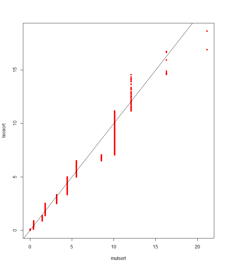
In Figure 4 we see that there are steps of different sizes, where some come from positive values of the signed log-likelihood and some come from negative values.
Refer to caption
Figure 4: A QQ-plot of a sample of the G2superscript𝐺2G^{2}-statistic from the contingency table IIIversus a sample from a χ2superscript𝜒2\chi^{2}-distribution with two degrees of freedom. the sample size in this simulation is 100 000.

To deminish such fluctuations we can make an asymmetric continuity correction as proposed by Gyërfi, Harremoës and Tusnády [14]. Such continuity correction will lead to a much closer fit to a χ2superscript𝜒2\chi^{2}-distribution, but it implies that the plugin estimate of mutual information has to be replaced by another expression and is thus not within the scope of this paper. Therefore the following examples will focus on symmetric contingency tables.

One may wonder if our observations are also true if there is more than one degree of freedom. It turns out out to be a more complicated question with no definite answer. We will illustrate this by two examples.

Example 20.

In this example we consider the contingency table III.

18 18 18 54
18 18 18 54
36 36 36 108
TABLE III: Contingency table with expected values and marginal counts.

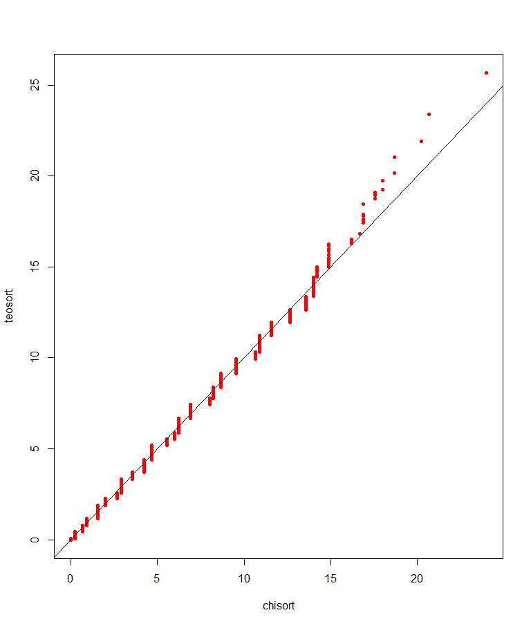
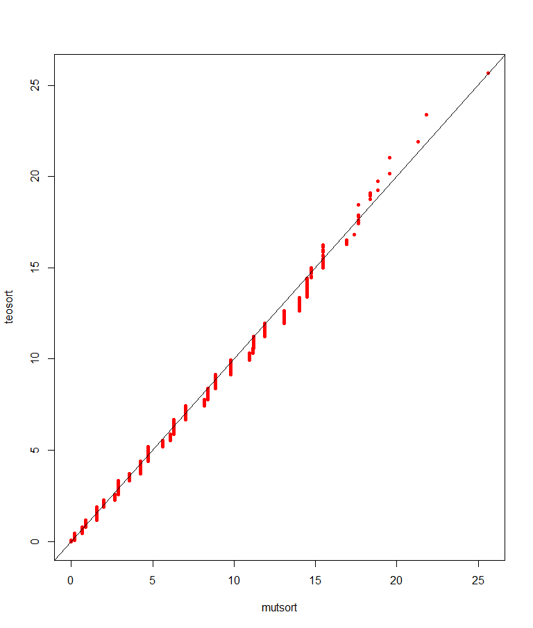
Due to the symmetry we do not get signicant interference between fluctuations in different direction. Both the distribution of the χ2superscript𝜒2\chi^{2}-statistic, the distribution of mutual information, and the theoretical χ2superscript𝜒2\chi^{2}-distribution have been simulated with a sample size equal to one million. In Figure 5 we see that the intersection property holds for mutual information , and in Figure 6that the χ2superscript𝜒2\chi^{2}-statistic systematically gives values that are too small for large deviation levels.
Refer to caption
Figure 5: A QQ-plot of a sample of the G2superscript𝐺2G^{2}-statistic from the contingency table IIIversus a sample from a χ2superscript𝜒2\chi^{2}-distribution with two degrees of freedom. the sample size in this simulation is 100 000.
Refer to caption
Figure 6: A QQ-plot of a sample of the χ2superscript𝜒2\chi^{2}-statistic from the contingency table IIIversus a sample from a χ2superscript𝜒2\chi^{2}-distribution with two degrees of freedom. the sample size in this simulation is 100 000.
Example 21.

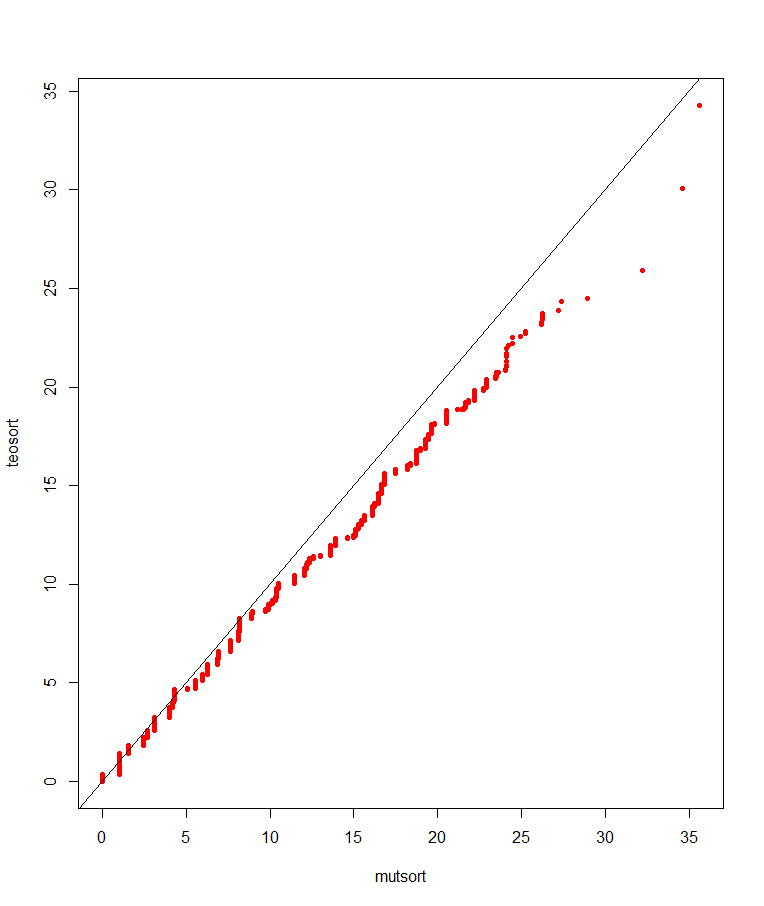
For the contingency table IV the sample size is relatively small compared with the number of degrees of freedom. In Figure 7 we see that the χ2superscript𝜒2\chi^{2}-statistic has a sligthly smaller vaue than the theoretical distribution while the mutual information is systematically too large for large deviations in Figure 8.
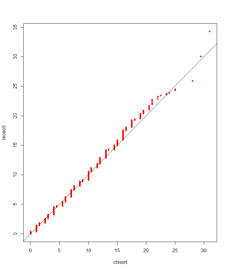
Refer to caption
Figure 7: A QQ-plot of a sample of the χ2superscript𝜒2\chi^{2}-statistic from the contingency table IV versus a sample from a χ2superscript𝜒2\chi^{2}-distribution with two degrees of freedom. the sample size in this simulation is 100 000.
4 4 4 12
4 4 4 12
4 4 4 12
12 12 12 36
TABLE IV: Contingency table with expected values and marginal counts.
Refer to caption
Figure 8: A QQ-plot of a sample of the χ2superscript𝜒2\chi^{2}-statistic from the contingency table IVversus a sample from a χ2superscript𝜒2\chi^{2}-distribution with two degrees of freedom. the sample size in this simulation is 100 000.

The tendency is that mutual information is better for large deviations and χ2superscript𝜒2\chi^{2} is better if the sample size is large compared with the degrees of freedom. The last problem can be corrected by ’smoothing’ by a rate distortion test as suggested in [15], but both continuity corrections and rate distortion tests just tell that there are good alternative to χ2superscript𝜒2\chi^{2} and mutual information. Looking at the behavior of such alternatives is not relevant if the question how to choose between χ2superscript𝜒2\chi^{2}and mutual information. We see that if there are more than one degree of freedom several effects point in opposite directions, so it might be more important to reash a better understanding of the situation where there is one degree of freedom before trying to generalize the results about one degree of freedom.