Local instabilities in magnetized rotational flows: A short-wavelength approach

Abstract

We perform a local stability analysis of rotational flows in the presence of a constant vertical magnetic field and an azimuthal magnetic field with a general radial dependence. Employing the short-wavelength approximation we develop a unified framework for the investigation of the standard, the helical, and the azimuthal version of the magnetorotational instability, as well as of current-driven kink-type instabilities. Considering the viscous and resistive setup, our main focus is on the case of small magnetic Prandtl numbers which applies, e.g., to liquid metal experiments but also to the colder parts of accretion disks. We show that the inductionless versions of MRI that were previously thought to be restricted to comparably steep rotation profiles extend well to the Keplerian case if only the azimuthal field slightly deviates from its current-free (in the fluid) profile. We find an explicit criterion separating the pure azimuthal inductionless magnetorotational instability from the regime where this instability is mixed with the Tayler instability. We further demonstrate that for particular parameter configurations the azimuthal MRI originates as a result of a dissipation-induced instability of the Chandrasekhar’s equipartition solution of ideal magnetohydrodynamics.

1 Introduction

The interaction of rotational flows and magnetic fields is of fundamental importance for many geo- and astrophysical problems (Rüdiger, Kitchatinov & Hollerbach, 2013). On one hand, rotating cosmic bodies, such as planets, stars, and galaxies are known to generate magnetic fields by means of the hydromagnetic dynamo effect. Magnetic fields, in turn, can destabilize rotating flows that would be otherwise hydrodynamically stable. This effect is particularly important for accretion disks in active galactic nuclei, dwarf novae and protoplanetary systems, where it allows for the tremendous enhancement of outward directed angular momentum transport that is necessary to explain the typical mass flow rates onto the respective central objects. Although this magnetorotational instability (MRI), as we call it now, had been discovered already in 1959 by Velikhov (Velikhov, 1959) and then confirmed in 1960 by Chandrasekhar (Chandrasekhar, 1960), it was left to Balbus & Hawley (1991) to point out its relevance for astrophysical accretion processes. Their seminal paper has inspired many investigations related to the action of MRI in active galactic nuclei (Krolik, 1998), X-ray binaries (Done, Gierlinski & Kubota, 2007), protoplanetary disks (Armitage, 2011), stars (Kagan & Wheeler, 2014), and even planetary cores (Petitdemange, Dormy & Balbus, 2008).

An interesting question concerns the non-trivial interplay of the hydromagnetic dynamo effect and magnetically triggered flow instabilities. For a long time, dynamo research had been focussed on how a prescribed flow can produce a magnetic field and, to a lesser extent, on how the self-excitation process saturates when the magnetic field becomes strong enough to act against the source of its own generation. Similarly, most of the early MRI studies have assumed some prescribed magnetic field, e.g., a purely axial or a purely azimuthal field, to assess its capability for triggering instabilities and turbulent angular momentum transport in the flow. Nowadays, however, we witness an increasing interest in treating the dynamo effect and instabilities in magnetized flows in a more self-consistent manner. Combining both processes one can ask for the existence of “self-creating dynamos” (Fuchs, Rädler & Rheinhardt, 1999), i.e. dynamos whose magnetic field triggers, at least partly, the flow structures that are responsible for its self-excitation.

A paradigm of such an essentially non-linear dynamo problem is the case of an accretion disk without any externally applied axial magnetic field. In this case the magnetic field can only be produced in the disk itself, very likely by a periodic MRI dynamo process (Herault et al., 2011) or some sort of an $\alpha-\Omega$ dynamo (Brandenburg et al., 1995), the $\alpha$ part of which relies on the turbulent flow structure arising due to the MRI. Such a closed loop of magnetic field self-excitation and MRI has attracted much attention in the past, though with many unsolved questions concerning numerical convergence (Fromang & Papaloizou, 2007), the influence of disk stratification (Shi, Krolik & Hirose, 2010), and the role of boundary conditions for the magnetic field (Käpylä & Korpi, 2011).

In problems of that kind, a key role is played by the so-called magnetic Prandtl number ${\rm Pm}=\nu/\eta$, i.e. the ratio of the viscosity $\nu$ of the fluid to its magnetic diffusivity $\eta=({\mu}_{0}\sigma)^{-1}$ (with ${\mu}_{0}$ denoting the magnetic permeability of free space and $\sigma$ the conductivity). For the case of an axially applied field, a first systematic study of the ${\rm Pm}$-dependence of the growth rate and the angular momentum transport coefficient was carried out by Lesur & Longaretti (2007). The closed-loop MRI-dynamo process, which seems to work well for ${\rm Pm}=O(1)$ (Herault et al., 2011), is much more intricate for small values of $\rm Pm$, as they are typical for the outer parts of accretion disks around black holes and for protoplanetary disks. At least for stratified disks, Oishi & Mac Low (2011) have recently claimed evidence for a critical magnetic Reynolds number ${\rm Rm}_{\rm crit}$ in the order of 3000 that is mainly independent of ${\rm Pm}$. A somewhat higher value of ${\rm Rm}_{\rm crit}$ had been found earlier by Fleming, Stone & Hawley (2000) when considering resistivity while still neglecting viscous effects.

Another paradigm of the interplay of self-excitation and magnetically triggered instabilities is the so-called Tayler-Spruit dynamo as proposed by Spruit (2002). In this particular (and controversially discussed) model of stellar magnetic field generation, the $\Omega$ part of the dynamo process (to produce toroidal field from poloidal field) is played, as usual, by the differential rotation, while the $\alpha$ part (to produce poloidal from toroidal field) is taken over by the flow structure arising from the kink-type Tayler instability (Tayler, 1973) that sets in when the toroidal field acquires a critical strength to overcome stable stratification.

At small values of $\rm Pm$, both dynamo and MRI related problems are very hard to treat numerically. This has to do with the fact that both phenomena rely on induction effects which require some finite magnetic Reynolds number. This number is the ratio of magnetic field production by the velocity to magnetic field dissipation due to Joule heating. For a fluid flow with typical size $L$ and typical velocity $V$ it can be expressed as ${\rm Rm}=\mu_{0}\sigma LV$. The numerical difficulty for small ${\rm Pm}$ problems arises then from the relation that the hydrodynamic Reynolds number, i.e. $\rm Re=Pm^{-1}Rm$, becomes very large, so that extremely fine structures have to be resolved. Furthermore, for MRI problems it is additionally necessary that the magnetic Lundquist number, which is simply a magnetic Reynolds number based on the Alfvén velocity $v_{A}$, i.e. $S=\mu_{0}\sigma Lv_{A}$, must also be in the order of 1.

A complementary way to study the interaction of rotating flows and magnetic field at small $\rm{Pm}$ and comparably large $\rm{Rm}$ is by means of liquid metal experiments. As for the dynamo problem, quite a number of experiments have been carried out (Stefani, Gailitis & Gerbeth, 2008). Up to present, magnetic field self-excitation has been attained in the liquid sodium experiments in Riga (Gailitis et al., 2000), Karlsruhe (Müller & Stieglitz, 2000), and Cadarache (Monchaux et al., 2007). Closely related to these dynamo experiments, some groups have also attempted to explore the standard version of MRI (SMRI), which corresponds to the case that a purely vertical magnetic field is being applied to the flow (Sisan et al., 2004; Nornberg et al., 2010). Recently, the current-driven, kink-type Tayler instability was identified in a liquid metal experiment (Seilmayer et al., 2012), the findings of which were numerically confirmed in the framework of an integro-differential equation approach by Weber et al. (2013).

With view on the peculiarities to do numerics, and experiments, on the standard version of MRI at low $\rm Pm$, it came as a big surprise when Hollerbach & Rüdiger (2005) showed that the simultaneous application of an axial and an azimuthal magnetic field can change completely the parameter scaling for the onset of MRI. For $B_{\phi}/B_{z}\sim 1$, the helical MRI (HMRI), as we call it now, was shown to work even in the inductionless limit (Priede, 2011; Kirillov & Stefani, 2011), ${\rm Pm}=0$, and to be governed by the Reynolds number ${\rm Re}={\rm Rm}{\rm Pm}^{-1}$ and the Hartmann number ${\rm Ha}=S{\rm Pm}^{-1/2}$, quite in contrast to standard MRI (SMRI) that was known to be governed by ${\rm Rm}$ and $S$ (Ji et al., 2001).

Very soon, however, the enthusiasm about this new inductionless version of MRI cooled down when Liu et al. (2006) showed that HMRI would only work for relatively steep rotation profiles, see also (Ji & Balbus, 2013). Using a short-wavelength approximation, they were able to identify a minimum steepness of the rotation profile $\Omega(R)$, expressed by the Rossby number ${\rm Ro}:=R(2\Omega)^{-1}\partial\Omega/\partial R<{\rm Ro}_{\rm LLL}=2(1{-}\sqrt{2})\approx-0.828$. This limit, which we will call the lower Liu limit (LLL) in the following, implies that for $B_{\phi}(R)\propto 1/R$ the inductionless HMRI does not extend to the Keplerian case, characterized by ${\rm Ro}_{\rm Kep}=-3/4$. Interestingly, Liu et al. (2006) found also a second threshold of the Rossby number, which we call the upper Liu limit (ULL), at ${\rm Ro}_{\rm ULL}=2(1{+}\sqrt{2})\approx+4.828$. This second limit, which predicts a magnetic destabilization of extremely stable flows with strongly increasing angular frequency, has attained nearly no attention up to present, but will play an important role in the present paper.

As for the general relation between HMRI and SMRI, two apparently contradicting observations have to be mentioned. On one hand, the numerical results of Hollerbach & Rüdiger (2005) had clearly demonstrated a continuous and monotonic transition between HMRI and SMRI. On the other hand, HMRI was identified by Liu et al. (2006) as a weakly destabilized inertial oscillation, quite in contrast to the SMRI which represents a destabilized slow magneto-Coriolis wave. Only recently, this paradox was resolved by showing that the transition involves a spectral exceptional point at which the inertial wave branch coalesces with the branch of the slow magneto-Coriolis wave (Kirillov & Stefani, 2010).

The significance of the LLL, together with a variety of further predicted parameter dependencies, was experimentally confirmed in the PROMISE facility, a Taylor-Couette cell working with a low ${\rm Pm}$ liquid metal (Stefani et al., 2006, 2007, 2009). Present experimental work at the same device (Seilmayer et al., 2014) aims at the characterization of the azimuthal MRI (AMRI), a non-axisymmetric “relative” of the axisymmetric HMRI, which dominates at large ratios of $B_{\phi}$ to $B_{z}$ (Hollerbach et al., 2010). However, AMRI as well as inductionless MRI modes with any other azimuthal wavenumber (which may be relevant at small values of $B_{\phi}/B_{z}$), seem also to be constrained by the LLL as recently shown in a unified treatment of all inductionless versions of MRI by Kirillov et al. (2012).

Actually, it is this apparent failure of HMRI, and AMRI, to apply to Keplerian profiles that has prevented a wider acceptance of those inductionless forms of MRI in the astrophysical community. Given the close proximity of the LLL ($\approx-0.83$) and the Keplerian Rossby number ($-0.75$), it is certainly worthwhile to ask whether any physically sensible modification would allow HMRI to extend to Keplerian flows.

Quite early, the validity of the LLL for $B_{\phi}(R)\propto 1/R$ had been questioned by Rüdiger & Hollerbach (2007). For the convective instability, they found an extension of the LLL to the Keplerian value in global simulations when at least one of the radial boundary conditions was assumed electrically conducting. Later, though, by extending the study to the absolute instability for the traveling HMRI waves, the LLL was vindicated even for such modified electrical boundary conditions by Priede (2011). Kirillov & Stefani (2011) made a second attempt by investigating HMRI for non-zero, but low $S$. For $B_{\phi}(R)\propto 1/R$ it was found that the essential HMRI mode extends from $S=0$ only to a value $S\approx 0.618$, and allows for a maximum Rossby number of ${\rm Ro}\approx-0.802$ which is indeed slightly above the LLL, yet below the Keplerian value.

A third possibility may arise when considering that saturation of MRI could lead to modified flow structures with parts of steeper shear, sandwiched with parts of shallower shear (Umurhan, 2010).

A recent letter (Kirillov & Stefani, 2013) has suggested another way of extending the range of applicability of the inductionless versions of MRI to Keplerian profiles, and beyond. Rather than relying on modified electrical boundary conditions, or on locally steepened $\Omega(R)$ profiles, we have evaluated $B_{\phi}(R)$ profiles that are flatter than $1/R$. The main physical idea behind this attempt is the following: assume that in some low-${\rm Pm}$ regions, characterized by $S<<1$ so that standard MRI is reliably suppressed, ${\rm Rm}$ is still sufficiently large for inducing significant azimuthal magnetic fields, either from a prevalent axial field $B_{z}$ or by means of a dynamo process without any prescribed $B_{z}$. Note that $B_{\phi}\propto 1/R$ would only appear in the extreme case of an isolated axial current, while the other extreme case, $B_{\phi}\propto R$, would correspond to the case of a homogeneous axial current density in the fluid which is already prone to the kink-type Tayler instability (Seilmayer et al., 2012), even at ${\rm Re}=0$.

Imagine now a real accretion disk with its complicated conductivity distributions in radial and axial direction. For such real disks a large variety of intermediate $B_{\phi}(R)$ profiles between the extreme cases $\propto 1/R$ and $\propto R$ is well conceivable. Instead of going into those details, one can ask which $B_{\phi}(R)$ profiles could make HMRI a viable mechanism for destabilizing Keplerian rotation profiles. By defining an appropriate magnetic Rossby number ${\rm Rb}$ we showed that the instability extends well beyond the LLL, even reaching ${\rm Ro}=0$ when going to ${\rm Rb}=-0.5$. It should be noted that in this extreme case of uniform rotation the only available energy source of the instability is the magnetic field. Going then over into the region of positive ${\rm Ro}$ in the ${\rm Ro}-{\rm Rb}$ plane, we found a natural connection with the ULL which was a somewhat mysterious conundrum up to present.

The present paper represents a significant extension of the short letter (Kirillov & Stefani, 2013). In the first instance, we will present a detailed derivation of the dispersion relation for arbitrary azimuthal modes in viscous, resistive rotational flows under the influence of a constant axial and a superposed azimuthal field of arbitrary radial dependence. For this purpose, we employ general short-wavelength asymptotic series following Eckhoff (1981, 1987), Bayly (1988), Lifschitz (1991), Lifschitz & Hameiri (1991), Friedlander & Vishik (1995), Vishik & Friedlander (1998), Hattori & Fukumoto (2003), and Friedlander & Lipton-Lifschitz (2003) as well as a WKB approach of Kirillov & Stefani (2010).

Second, we will discuss in much more detail the stability map in the ${\rm Ro}-{\rm Rb}$-plane in the inductionless case of vanishing magnetic Prandtl number. For various limits we will discuss a number of strict results concerning the stability threshold and the growth rates. Special focus will be laid on the role that is played by the line ${\rm Ro}={\rm Rb}$, and by the point ${\rm Ro}={\rm Rb}=-2/3$ in particular.

Third, we will elaborate the dependence of the instability on the azimuthal wavenumber and on the ratio of the axial and radial wavenumbers and prove that the pattern of instability domains in the case of very small, but finite $\rm Pm$, is governed by a periodic band structure found in the inductionless limit.

Next, we will establish a connection between dissipation-induced destabilization of Chandrasekhar’s equipartition solution (a special solution for which the fluid velocity is parallel to the direction of the magnetic field and magnetic and kinetic energies are finite and equal (Chandrasekhar, 1956, 1961)) and the azimuthal MRI, and we will explore the links between the Tayler instability and AMRI.

Last, but not least, we will delineate some possible astrophysical and experimental consequences of our findings, although a comprehensive discussions of the corresponding details must be left for future work.

2 Mathematical setting

2.1 Non-linear equations

The standard set of non-linear equations of dissipative incompressible magnetohydrodynamics consists of the Navier-Stokes equation for the fluid velocity $\boldsymbol{u}$ and of the induction equation for the magnetic field $\boldsymbol{B}$

$$\frac{\partial\boldsymbol{u}}{\partial t}+\boldsymbol{u}\boldsymbol{\cdot}\boldsymbol{\nabla}\boldsymbol{u}-\frac{1}{\mu_{0}\rho}\boldsymbol{B}\boldsymbol{\cdot}\boldsymbol{\nabla}\boldsymbol{B}+\frac{1}{\rho}\boldsymbol{\nabla}P-\nu\boldsymbol{\nabla}^{2}\boldsymbol{u}=0,$$

$$\frac{\partial\boldsymbol{B}}{\partial t}+\boldsymbol{u}\boldsymbol{\cdot}\boldsymbol{\nabla}\boldsymbol{B}-\boldsymbol{B}\boldsymbol{\cdot}\boldsymbol{\nabla}\boldsymbol{u}-\eta\boldsymbol{\nabla}^{2}\boldsymbol{B}=0,$$ (1)

where $P=p+\frac{\boldsymbol{B}^{2}}{2\mu_{0}}$ is the total pressure, $p$ is the hydrodynamic pressure, $\rho=const$ the density, $\nu=const$ the kinematic viscosity, $\eta=(\mu_{0}\sigma)^{-1}$ the magnetic diffusivity, $\sigma$ the conductivity of the fluid, and $\mu_{0}$ the magnetic permeability of free space. Additionally, the mass continuity equation for incompressible flows and the solenoidal condition for the magnetic induction yield

$$\boldsymbol{\nabla}\boldsymbol{\cdot}\boldsymbol{u}=0,\quad\boldsymbol{\nabla}\boldsymbol{\cdot}\boldsymbol{B}=0.$$ (2)

2.2 Steady state

We consider the rotational fluid flow in the gap between the radii $R_{1}$ and $R_{2}>R_{1}$, with an imposed magnetic field sustained by electrical currents. Introducing the cylindrical coordinates $(R,\phi,z)$ we consider the stability of a steady-state background liquid flow with the angular velocity profile $\Omega(R)$ in helical background magnetic field (a magnetized Taylor-Couette (TC) flow)

$$\boldsymbol{u}_{0}(R)=R\,\Omega(R)\,\boldsymbol{e}_{\phi},\quad p=p_{0}(R),\quad\boldsymbol{B}_{0}(R)=B_{\phi}^{0}(R)\boldsymbol{e}_{\phi}+B_{z}^{0}\boldsymbol{e}_{z}.$$ (3)

Note that if the azimuthal component is produced by an axial current $I$ confined to $R<R_{1}$, then

$$B_{\phi}^{0}(R)=\frac{\mu_{0}I}{2\pi R}.$$ (4)

Introducing the hydrodynamic Rossby number $({\rm Ro})$ by means of the relation

$${\rm Ro}:=\frac{R}{2\Omega}\partial_{R}\Omega,$$ (5)

we find that the solid body rotation corresponds to ${\rm Ro}=0$, the Keplerian rotation to ${\rm Ro}=-3/4$, whereas the velocity profile $\Omega(R)\sim R^{-2}$ corresponds to ${\rm Ro}=-1$. Note that although Keplerian rotation is not possible globally in TC-flow, an approximate Keplerian profile can locally be achieved.

Similarly, following Kirillov & Stefani (2013) we define the magnetic Rossby number

$${\rm Rb}:=\frac{R}{2B_{\phi}^{0}R^{-1}}\partial_{R}(B_{\phi}^{0}R^{-1}).$$ (6)

${\rm Rb}=0$ results from a linear dependence of the magnetic field on the radius, $B_{\phi}^{0}(R)\propto R$, as it would be produced by a homogeneous axial current in the fluid. ${\rm Rb}=-1$ corresponds to the radial dependence given by Eq. (4). Note that the logarithmic derivatives $\alpha$ and $\beta$ introduced in the work by Ogilvie & Pringle (1996) are nothing else but the doubled hydrodynamic and magnetic Rossby numbers: $\alpha=2{\rm Ro}$, $\beta=2{\rm Rb}$.

2.3 Linearization with respect to non-axisymmetric perturbations

To describe natural oscillations in the neighborhood of the magnetized Taylor-Couette flow we linearize equations (2.1)-(2) in the vicinity of the stationary solution (3) assuming general perturbations $\boldsymbol{u}=\boldsymbol{u}_{0}+\boldsymbol{u}^{\prime}$, $p=p_{0}+p^{\prime}$, and $\boldsymbol{B}=\boldsymbol{B}_{0}+\boldsymbol{B}^{\prime}$ and leaving only the terms of first order with respect to the primed quantities:

$$\partial_{t}\boldsymbol{u}^{\prime}+\boldsymbol{u}_{0}\boldsymbol{\cdot}\boldsymbol{\nabla}\boldsymbol{u}^{\prime}+\boldsymbol{u}^{\prime}\boldsymbol{\cdot}\boldsymbol{\nabla}\boldsymbol{u}_{0}-\frac{1}{\rho\mu_{0}}\left(\boldsymbol{B}_{0}\boldsymbol{\cdot}\boldsymbol{\nabla}\boldsymbol{B}^{\prime}{+}\boldsymbol{B}^{\prime}\boldsymbol{\cdot}\boldsymbol{\nabla}\boldsymbol{B}_{0}\right)-\nu\boldsymbol{\nabla}^{2}\boldsymbol{u}^{\prime}=$$

$$-\frac{1}{\rho}\boldsymbol{\nabla}p^{\prime}-\frac{1}{\rho\mu_{0}}\boldsymbol{\nabla}(\boldsymbol{B}_{0}\boldsymbol{\cdot}\boldsymbol{B}^{\prime}),$$

$$\partial_{t}\boldsymbol{B}^{\prime}+\boldsymbol{u}_{0}\boldsymbol{\cdot}\boldsymbol{\nabla}\boldsymbol{B}^{\prime}+\boldsymbol{u}^{\prime}\boldsymbol{\cdot}\boldsymbol{\nabla}\boldsymbol{B}_{0}-\boldsymbol{B}_{0}\boldsymbol{\cdot}\boldsymbol{\nabla}\boldsymbol{u}^{\prime}-\boldsymbol{B}^{\prime}\boldsymbol{\cdot}\boldsymbol{\nabla}\boldsymbol{u}_{0}-\eta\boldsymbol{\nabla}^{2}\boldsymbol{B}^{\prime}=0,$$ (7)

where the perturbations fulfil the constraints

$$\boldsymbol{\nabla}\boldsymbol{\cdot}\boldsymbol{u}^{\prime}=0,\quad\boldsymbol{\nabla}\boldsymbol{\cdot}\boldsymbol{B}^{\prime}=0.$$ (8)

Note that by adding/subtracting the second of equations (2.3) divided by $\sqrt{\rho\mu_{0}}$ to/from the first one yields the linearized equations in a more symmetrical Elsasser form; in the ideal MHD case they were derived, e.g. by Friedlander & Vishik (1995).

Introducing the gradients of the background fields represented by the two $3\times 3$ matrices

$$\mathcal{U}(R)=\boldsymbol{\nabla}\boldsymbol{u}_{0}=\Omega\left(\begin{array}[]{ccc}0&-1&0\\ 1+2{\rm Ro}&0&0\\ 0&0&0\\ \end{array}\right),$$ (12)

$$\mathcal{B}(R)=\boldsymbol{\nabla}\boldsymbol{B}_{0}=\frac{B_{\phi}^{0}}{R}\left(\begin{array}[]{ccc}0&-1&0\\ 1+2{\rm Rb}&0&0\\ 0&0&0\\ \end{array}\right),$$ (16)

we write the linearized equations of motion in the form

$$(\partial_{t}+\mathcal{U}+\boldsymbol{u}_{0}\boldsymbol{\cdot}\boldsymbol{\nabla})\boldsymbol{u}^{\prime}-\frac{1}{\rho\mu_{0}}\left(\mathcal{B}+\boldsymbol{B}_{0}\boldsymbol{\cdot}\boldsymbol{\nabla}\right)\boldsymbol{B}^{\prime}-\nu\boldsymbol{\nabla}^{2}\boldsymbol{u}^{\prime}+\frac{1}{\rho}\boldsymbol{\nabla}p^{\prime}+\frac{1}{\rho\mu_{0}}\boldsymbol{\nabla}(\boldsymbol{B}_{0}\boldsymbol{\cdot}\boldsymbol{B}^{\prime})=0,$$

$$(\partial_{t}-\mathcal{U}+\boldsymbol{u}_{0}\boldsymbol{\cdot}\boldsymbol{\nabla})\boldsymbol{B}^{\prime}+(\mathcal{B}-\boldsymbol{B}_{0}\boldsymbol{\cdot}\boldsymbol{\nabla})\boldsymbol{u}^{\prime}-\eta\boldsymbol{\nabla}^{2}\boldsymbol{B}^{\prime}=0.$$ (17)

3 Geometrical optics equations

Following Eckhoff (1981), Lifschitz (1989, 1991) and Friedlander & Lipton-Lifschitz (2003), we seek for solutions of the linearized equations (2.3) in terms of the formal asymptotic series with respect to the small parameter $\epsilon$, $0<\epsilon\ll 1$:

$$\boldsymbol{u}^{\prime}(\boldsymbol{x},t,\epsilon)=e^{i\Phi(\boldsymbol{x},t)/\epsilon}\left(\boldsymbol{u}^{(0)}(\boldsymbol{x},t)+\epsilon\boldsymbol{u}^{(1)}(\boldsymbol{x},t)\right)+\epsilon\boldsymbol{u}^{(r)}(\boldsymbol{x},t),$$

$$\boldsymbol{B}^{\prime}(\boldsymbol{x},t,\epsilon)=e^{i\Phi(\boldsymbol{x},t)/\epsilon}\left(\boldsymbol{B}^{(0)}(\boldsymbol{x},t)+\epsilon\boldsymbol{B}^{(1)}(\boldsymbol{x},t)\right)+\epsilon\boldsymbol{B}^{(r)}(\boldsymbol{x},t),$$

$$p^{\prime}(\boldsymbol{x},t,\epsilon)=e^{i\Phi(\boldsymbol{x},t)/\epsilon}\left(p^{(0)}(\boldsymbol{x},t)+\epsilon p^{(1)}(\boldsymbol{x},t)\right)+\epsilon p^{(r)}(\boldsymbol{x},t),$$ (18)

where $\boldsymbol{x}$ is a vector of coordinates, $\Phi$ is a real-valued scalar function that represents the ‘fast’ phase of oscillations, and $\boldsymbol{u}^{(j)}$, $\boldsymbol{B}^{(j)}$, and $p^{(j)}$, $j=0,1,r$ are ‘slow’ complex-valued amplitudes with the index $r$ denoting residual terms.

Following Landman & Saffman (1987), Lifschitz (1991), Dobrokhotov & Shafarevich (1992), and Eckhardt & Yao (1995) we assume further in the text that $\nu=\epsilon^{2}\tilde{\nu}$ and $\eta=\epsilon^{2}\tilde{\eta}$ and introduce the derivative along the fluid stream lines

$$\frac{D}{Dt}:=\partial_{t}+\boldsymbol{u}_{0}\boldsymbol{\cdot}\boldsymbol{\nabla}.$$ (19)

Substituting expansions (3) into equations (2.3), taking into account the identity

$$(\boldsymbol{A}\boldsymbol{\cdot}\boldsymbol{\nabla})\Phi\boldsymbol{B}=(\boldsymbol{A}\boldsymbol{\cdot}\boldsymbol{\nabla}\Phi)\boldsymbol{B}+\Phi(\boldsymbol{A}\boldsymbol{\cdot}\boldsymbol{\nabla})\boldsymbol{B},$$ (20)

as well as the relation

$$\boldsymbol{\nabla}^{2}(\boldsymbol{u}^{\prime})=e^{i\frac{\Phi}{\epsilon}}\left(\boldsymbol{\nabla}^{2}+i\frac{2}{\epsilon}(\boldsymbol{\nabla}\Phi\boldsymbol{\cdot}\boldsymbol{\nabla})+i\frac{\boldsymbol{\nabla}^{2}\Phi}{\epsilon}-\frac{(\boldsymbol{\nabla}\Phi)^{2}}{\epsilon^{2}}\right)(\boldsymbol{u}^{(0)}+\epsilon\boldsymbol{u}^{(1)})+\epsilon\boldsymbol{\nabla}^{2}(\boldsymbol{u}^{(r)}),$$ (21)

collecting terms at $\epsilon^{-1}$ and $\epsilon^{0}$ we arrive at the system of local partial differential equations (cf. Friedlander & Vishik (1995))

$$\frac{D\Phi}{Dt}\boldsymbol{u}^{(0)}-\frac{1}{\rho\mu_{0}}(\boldsymbol{B}_{0}\boldsymbol{\cdot}\boldsymbol{\nabla}\Phi)\boldsymbol{B}^{(0)}+\frac{\boldsymbol{\nabla}\Phi}{\rho}\left(p^{(0)}+\frac{1}{\mu_{0}}(\boldsymbol{B}_{0}\boldsymbol{\cdot}\boldsymbol{B}^{(0)})\right)=0,$$ (22)

$$\frac{D\Phi}{Dt}\boldsymbol{B}^{(0)}-(\boldsymbol{B}_{0}\boldsymbol{\cdot}\boldsymbol{\nabla}\Phi)\boldsymbol{u}^{(0)}=0,$$

$$i\frac{D\Phi}{Dt}\boldsymbol{u}^{(1)}+\left(\frac{D}{Dt}+\tilde{\nu}(\boldsymbol{\nabla}\Phi)^{2}+\mathcal{U}\right)\boldsymbol{u}^{(0)}-\frac{1}{\rho\mu_{0}}\left(\mathcal{B}+\boldsymbol{B}_{0}\boldsymbol{\cdot}\boldsymbol{\nabla}\right)\boldsymbol{B}^{(0)}-\frac{i}{\rho\mu_{0}}(\boldsymbol{B}_{0}\boldsymbol{\cdot}\boldsymbol{\nabla}\Phi)\boldsymbol{B}^{(1)}$$

$$+\frac{\boldsymbol{\nabla}}{\rho}\left(p^{(0)}+\frac{1}{\mu_{0}}(\boldsymbol{B}_{0}\boldsymbol{\cdot}\boldsymbol{B}^{(0)})\right)+i\frac{\boldsymbol{\nabla}\Phi}{\rho}\left(p^{(1)}+\frac{1}{\mu_{0}}(\boldsymbol{B}_{0}\boldsymbol{\cdot}\boldsymbol{B}^{(1)})\right)=0,$$

$$i\frac{D\Phi}{Dt}\boldsymbol{B}^{(1)}+\left(\frac{D}{Dt}+\tilde{\eta}(\boldsymbol{\nabla}\Phi)^{2}-\mathcal{U}\right)\boldsymbol{B}^{(0)}+(\mathcal{B}-\boldsymbol{B}_{0}\boldsymbol{\cdot}\boldsymbol{\nabla})\boldsymbol{u}^{(0)}-i(\boldsymbol{B}_{0}\boldsymbol{\cdot}\boldsymbol{\nabla}\Phi)\boldsymbol{u}^{(1)}=0.$$

From the solenoidality conditions (8) it follows that

$$\boldsymbol{u}^{(0)}\boldsymbol{\cdot}\boldsymbol{\nabla}\Phi=0,\quad\boldsymbol{\nabla}\boldsymbol{\cdot}\boldsymbol{u}^{(0)}+i\boldsymbol{u}^{(1)}\boldsymbol{\cdot}\boldsymbol{\nabla}\Phi=0,$$

$$\boldsymbol{B}^{(0)}\boldsymbol{\cdot}\boldsymbol{\nabla}\Phi=0,\quad\boldsymbol{\nabla}\boldsymbol{\cdot}\boldsymbol{B}^{(0)}+i\boldsymbol{B}^{(1)}\boldsymbol{\cdot}\boldsymbol{\nabla}\Phi=0.$$ (23)

Following Lifschitz (1991) we take the dot product of the first two of the equations (22) with $\boldsymbol{\nabla}\Phi$, $\boldsymbol{u}^{(0)}$, $\boldsymbol{B}^{(0)}$ and, in view of the constraints (3), arrive at the system

$$\frac{(\boldsymbol{\nabla}\Phi)^{2}}{\rho}\left(p^{(0)}+\frac{1}{\mu_{0}}(\boldsymbol{B}_{0}\boldsymbol{\cdot}\boldsymbol{B}^{(0)})\right)=0,$$

$$\frac{D\Phi}{Dt}\boldsymbol{B}^{(0)}\boldsymbol{\cdot}\boldsymbol{B}^{(0)}-(\boldsymbol{B}_{0}\boldsymbol{\cdot}\boldsymbol{\nabla}\Phi)\boldsymbol{u}^{(0)}\boldsymbol{\cdot}\boldsymbol{B}^{(0)}=0,$$

$$\frac{D\Phi}{Dt}\boldsymbol{B}^{(0)}\boldsymbol{\cdot}\boldsymbol{u}^{(0)}-(\boldsymbol{B}_{0}\boldsymbol{\cdot}\boldsymbol{\nabla}\Phi)\boldsymbol{u}^{(0)}\boldsymbol{\cdot}\boldsymbol{u}^{(0)}=0,$$

$$\frac{D\Phi}{Dt}\boldsymbol{u}^{(0)}\boldsymbol{\cdot}\boldsymbol{B}^{(0)}-\frac{1}{\rho\mu_{0}}\boldsymbol{B}^{(0)}\boldsymbol{\cdot}\boldsymbol{B}^{(0)}(\boldsymbol{B}_{0}\boldsymbol{\cdot}\boldsymbol{\nabla}\Phi)=0,$$

$$\frac{D\Phi}{Dt}\boldsymbol{u}^{(0)}\boldsymbol{\cdot}\boldsymbol{u}^{(0)}-\frac{1}{\rho\mu_{0}}\boldsymbol{B}^{(0)}\boldsymbol{\cdot}\boldsymbol{u}^{(0)}(\boldsymbol{B}_{0}\boldsymbol{\cdot}\boldsymbol{\nabla}\Phi)=0,$$ (24)

that has for $\boldsymbol{\nabla}\Phi\neq 0$, $\boldsymbol{B}^{(0)}\neq 0$, and $\boldsymbol{u}^{(0)}\neq 0$ a unique solution

$$p^{(0)}=-\frac{1}{\mu_{0}}(\boldsymbol{B}_{0}\boldsymbol{\cdot}\boldsymbol{B}^{(0)}),\quad\frac{D\Phi}{Dt}=0,\quad\boldsymbol{B}_{0}\boldsymbol{\cdot}\boldsymbol{\nabla}\Phi=0.$$ (25)

With the use of the relations (25) we simplify the last two of the equations (22) as

$$\left(\frac{D}{Dt}+\tilde{\nu}(\boldsymbol{\nabla}\Phi)^{2}+\mathcal{U}\right)\boldsymbol{u}^{(0)}-\frac{1}{\rho\mu_{0}}(\mathcal{B}+\boldsymbol{B}_{0}\boldsymbol{\cdot}\boldsymbol{\nabla})\boldsymbol{B}^{(0)}=-i\frac{\boldsymbol{\nabla}\Phi}{\rho}\left(p^{(1)}+\frac{1}{\mu_{0}}(\boldsymbol{B}_{0}\boldsymbol{\cdot}\boldsymbol{B}^{(1)})\right),$$

$$\left(\frac{D}{Dt}+\tilde{\eta}(\boldsymbol{\nabla}\Phi)^{2}-\mathcal{U}\right)\boldsymbol{B}^{(0)}+(\mathcal{B}-\boldsymbol{B}_{0}\boldsymbol{\cdot}\boldsymbol{\nabla})\boldsymbol{u}^{(0)}=0.$$ (26)

Multiplying the first of Eqs. (3) by $\boldsymbol{\nabla}\Phi$ from the left and then dividing both parts by $|\boldsymbol{\nabla}\Phi|^{2}$ we find an expression for $p^{(1)}+\frac{1}{\mu_{0}}(\boldsymbol{B}_{0}\boldsymbol{\cdot}\boldsymbol{B}^{(1)})$. Substituting it back to the right hand side of the first of Eqs. (3) and taking into account the constraints (3), we eliminate the pressure terms and transform this equation into

$$\left(\frac{D}{Dt}+\tilde{\nu}(\boldsymbol{\nabla}\Phi)^{2}+\mathcal{U}\right)\boldsymbol{u}^{(0)}-\frac{1}{\rho\mu_{0}}(\mathcal{B}+\boldsymbol{B}_{0}\boldsymbol{\cdot}\boldsymbol{\nabla})\boldsymbol{B}^{(0)}$$

$$=\frac{\boldsymbol{\nabla}\Phi}{|\boldsymbol{\nabla}\Phi|^{2}}\boldsymbol{\cdot}\left[\left(\frac{D}{Dt}+\mathcal{U}\right)\boldsymbol{u}^{(0)}-\frac{1}{\rho\mu_{0}}(\mathcal{B}+\boldsymbol{B}_{0}\boldsymbol{\cdot}\boldsymbol{\nabla})\boldsymbol{B}^{(0)}\right]{\boldsymbol{\nabla}\Phi},$$ (27)

quite in accordance with the standard procedure described, e.g., in Lifschitz (1991) and Vishik & Friedlander (1998). Differentiating the first of the identities (3) yields

$$\frac{D}{Dt}(\boldsymbol{\nabla}\Phi\boldsymbol{\cdot}\boldsymbol{u}^{(0)})=\frac{D\boldsymbol{\nabla}\Phi}{Dt}\boldsymbol{\cdot}\boldsymbol{u}^{(0)}+\boldsymbol{\nabla}\Phi\boldsymbol{\cdot}\frac{D\boldsymbol{u}^{(0)}}{Dt}=0.$$ (28)

Using the identity (28), we re-write Eq. (3) as follows

$$\left(\frac{D}{Dt}+\tilde{\nu}(\boldsymbol{\nabla}\Phi)^{2}+\mathcal{U}\right)\boldsymbol{u}^{(0)}-\frac{1}{\rho\mu_{0}}(\mathcal{B}+\boldsymbol{B}_{0}\boldsymbol{\cdot}\boldsymbol{\nabla})\boldsymbol{B}^{(0)}$$

$$=\frac{\boldsymbol{\nabla}\Phi}{|\boldsymbol{\nabla}\Phi|^{2}}\boldsymbol{\cdot}\left[\mathcal{U}\boldsymbol{u}^{(0)}-\frac{1}{\rho\mu_{0}}(\mathcal{B}+\boldsymbol{B}_{0}\boldsymbol{\cdot}\boldsymbol{\nabla})\boldsymbol{B}^{(0)}\right]\boldsymbol{\nabla}\Phi-\frac{\boldsymbol{\nabla}\Phi}{|\boldsymbol{\nabla}\Phi|^{2}}\frac{D\boldsymbol{\nabla}\Phi}{Dt}\boldsymbol{\cdot}\boldsymbol{u}^{(0)},$$

Now we take the gradient of the identity $D\Phi/Dt=0$:

$$\boldsymbol{\nabla}\partial_{t}\Phi+\boldsymbol{\nabla}(\boldsymbol{u}_{0}\boldsymbol{\cdot}\boldsymbol{\nabla})\Phi=\partial_{t}\boldsymbol{\nabla}\Phi+(\boldsymbol{u}_{0}\boldsymbol{\cdot}\boldsymbol{\nabla})\boldsymbol{\nabla}\Phi+\mathcal{U}^{T}\boldsymbol{\nabla}\Phi$$

$$=\frac{D}{Dt}\boldsymbol{\nabla}\Phi+\mathcal{U}^{T}\boldsymbol{\nabla}\Phi=0.$$ (29)

Denoting $\boldsymbol{k}=\boldsymbol{\nabla}\Phi$, we deduce from the phase equation (3) that

$$\frac{D\boldsymbol{k}}{Dt}=-\mathcal{U}^{T}\boldsymbol{k}.$$ (30)

Hence, the transport equations for the amplitudes (3) take the final form

$$\frac{D\boldsymbol{u}^{(0)}}{Dt}=-\left(\mathcal{I}-2\frac{\boldsymbol{k}\boldsymbol{k}^{T}}{|\boldsymbol{k}|^{2}}\right)\mathcal{U}\boldsymbol{u}^{(0)}-\tilde{\nu}|\boldsymbol{k}|^{2}\boldsymbol{u}^{(0)}+\frac{1}{\rho\mu_{0}}\left(\mathcal{I}-\frac{\boldsymbol{k}\boldsymbol{k}^{T}}{|\boldsymbol{k}|^{2}}\right)\left(\mathcal{B}+\boldsymbol{B}_{0}\boldsymbol{\cdot}\boldsymbol{\nabla}\right)\boldsymbol{B}^{(0)},$$

$$\frac{D\boldsymbol{B}^{(0)}}{Dt}=\mathcal{U}\boldsymbol{B}^{(0)}-\tilde{\eta}|\boldsymbol{k}|^{2}\boldsymbol{B}^{(0)}-(\mathcal{B}-\boldsymbol{B}_{0}\boldsymbol{\cdot}\boldsymbol{\nabla})\boldsymbol{u}^{(0)},$$ (31)

where $\mathcal{I}$ is a $3\times 3$ identity matrix.

Eqs. (3) are local partial differential equations analogous to those derived (in terms of Elsasser variables $\boldsymbol{u}^{(0)}\pm{\boldsymbol{B}^{(0)}}(\rho\mu_{0})^{-1/2}$) by Friedlander & Vishik (1995) who considered non-axisymmetric perturbation of a rotating flow of an ideal incompressible fluid which is a perfect electrical conductor in the presence of the azimuthal magnetic field of arbitrary radial and axial dependency, see Appendix A.

In the absence of the magnetic field these equations can be treated as ordinary differential equations with respect to the convective derivative (19) and thus are reduced to that of Eckhardt & Yao (1995) who considered stability of the viscous TC-flow. Note that the same form of the transport equations (with the different matrix $\mathcal{U}$) appears in the studies of elliptical instability by Landman & Saffman (1987) and of three-dimensional local instabilities of more general viscous and inviscid basic flows by Lifschitz (1991), Lifschitz & Hameiri (1991), and Dobrokhotov & Shafarevich (1992).

4 Dispersion relation of AMRI

In case when the axial field is absent, i.e. $B_{z}^{0}=0$, we can derive the dispersion relation of AMRI directly from the transport equations (3) according to the procedure described in Friedlander & Vishik (1995).

Let the orthogonal unit vectors $\boldsymbol{e}_{R}(t)$, $\boldsymbol{e}_{\phi}(t)$, and $\boldsymbol{e}_{z}(t)$ form a basis in a cylindrical coordinate system moving along the fluid trajectory. With $\boldsymbol{k}(t)=k_{R}\boldsymbol{e}_{R}(t)+k_{\phi}\boldsymbol{e}_{\phi}(t)+k_{z}\boldsymbol{e}_{z}(t)$, $\boldsymbol{u}(t)=u_{R}\boldsymbol{e}_{R}(t)+u_{\phi}\boldsymbol{e}_{\phi}(t)+u_{z}\boldsymbol{e}_{z}(t)$, and with the matrix $\mathcal{U}$ from (12), we find

$$\dot{\boldsymbol{e}}_{R}=\Omega(R){\bf e}_{\phi},\quad\dot{\boldsymbol{e}}_{\phi}=-\Omega(R)\boldsymbol{e}_{R}.$$ (32)

Hence, the equation (30) in the coordinate form is

$$\dot{k}_{R}=-R\partial_{R}\Omega k_{\phi},\quad\dot{k}_{\phi}=0,\quad\dot{k}_{z}=0.$$ (33)

According to Eckhardt & Yao (1995) and Friedlander & Vishik (1995), in order to study physically relevant and potentially unstable modes we have to choose bounded and asymptotically non-decaying solutions of the system (33). These correspond to $k_{\phi}\equiv 0$ and $k_{R}$ and $k_{z}$ time-independent. Note that when $B_{z}^{0}=0$ this solution is compatible with the constraint $\boldsymbol{B}_{0}\boldsymbol{\cdot}\boldsymbol{k}=0$ following from (25).

Denoting $\alpha=k_{z}|\boldsymbol{k}|^{-1}$, where $|\boldsymbol{k}|^{2}=k_{R}^{2}+k_{z}^{2}$, we find that $k_{R}k_{z}^{-1}=\sqrt{1-\alpha^{2}}\alpha^{-1}$ we write the local partial differential equations (3) for the amplitudes in the coordinate representation. Analogously to Friedlander & Vishik (1995), we single out the equations for the radial and azimuthal components of the fluid velocity and magnetic field by using the orthogonality condition ${B}_{R}^{(0)}k_{R}+{B}_{z}^{(0)}k_{z}=0$ that follows from (3):

$$\left(\partial_{t}{+}\Omega\partial_{\phi}{+}\widetilde{\nu}|\boldsymbol{k}|^{2}\right)u_{R}^{(0)}-2\alpha^{2}\Omega u_{\phi}^{(0)}+2\alpha^{2}\frac{B_{\phi}^{0}}{\rho\mu_{0}R}B_{\phi}^{(0)}-\frac{B_{\phi}^{0}}{R}\frac{\partial_{\phi}B_{R}^{(0)}}{\rho\mu_{0}}=0,$$

$$\left(\partial_{t}{+}\Omega\partial_{\phi}+\widetilde{\nu}|\boldsymbol{k}|^{2}\right)u_{\phi}^{(0)}+2\Omega(1{+}{\rm Ro})u_{R}^{(0)}-\frac{2}{\rho\mu_{0}}\frac{B_{\phi}^{0}}{R}(1{+}{\rm Rb})B_{R}^{(0)}-\frac{B_{\phi}^{0}}{R}\frac{\partial_{\phi}B_{\phi}^{(0)}}{\rho\mu_{0}}=0,$$

$$\left(\partial_{t}{+}\Omega\partial_{\phi}{+}\widetilde{\eta}|\boldsymbol{k}|^{2}\right)B_{R}^{(0)}-\frac{B_{\phi}^{0}}{R}\partial_{\phi}u_{R}^{(0)}=0,$$

$$\left(\partial_{t}{+}\Omega\partial_{\phi}{+}\widetilde{\eta}|\boldsymbol{k}|^{2}\right)B_{\phi}^{(0)}-2\Omega{\rm Ro}B_{R}^{(0)}+2{\rm Rb}\frac{B_{\phi}^{0}}{R}u_{R}^{(0)}-\frac{B_{\phi}^{0}}{R}\partial_{\phi}u_{\phi}^{(0)}=0.$$ (34)

According to Friedlander & Vishik (1995) a natural step is to seek for a solution to Eqs. (4) in the modal form $\boldsymbol{u}^{(0)}=\widehat{\boldsymbol{u}}e^{\gamma t+im\phi}$, $\boldsymbol{B}^{(0)}=\widehat{\boldsymbol{B}}e^{\gamma t+im\phi}$ in order to end up with the dispersion relation for the transport equations in case of AMRI:

$$(\gamma+im\Omega+\widetilde{\nu}|\boldsymbol{k}|^{2})\widehat{u}_{R}-2\alpha^{2}\Omega\widehat{u}_{\phi}+2\alpha^{2}\frac{B_{\phi}^{0}}{\rho\mu_{0}R}\widehat{B}_{\phi}-im\frac{B_{\phi}^{0}}{R}\frac{\widehat{B}_{R}}{\rho\mu_{0}}=0,$$

$$(\gamma+im\Omega+\widetilde{\nu}|\boldsymbol{k}|^{2})\widehat{u}_{\phi}+2\Omega(1+{\rm Ro})\widehat{u}_{R}-\frac{2}{\rho\mu_{0}}\frac{B_{\phi}^{0}}{R}(1+{\rm Rb})\widehat{B}_{R}-im\frac{B_{\phi}^{0}}{R}\frac{\widehat{B}_{\phi}}{\rho\mu_{0}}=0,$$

$$(\gamma+im\Omega+\widetilde{\eta}|\boldsymbol{k}|^{2})\widehat{B}_{R}-im\frac{B_{\phi}^{0}}{R}\widehat{u}_{R}=0,$$

$$(\gamma+im\Omega+\widetilde{\eta}|\boldsymbol{k}|^{2})\widehat{B}_{\phi}-2\Omega{\rm Ro}\widehat{B}_{R}+2{\rm Rb}\frac{B_{\phi}^{0}}{R}\widehat{u}_{R}-im\frac{B_{\phi}^{0}}{R}\widehat{u}_{\phi}=0.$$ (35)

Introducing the viscous and resistive frequencies and the $\rm Alfv\acute{e}n$ angular velocity (Ogilvie & Pringle, 1996) corresponding to the azimuthal magnetic field:

$$\omega_{\nu}=\widetilde{\nu}|\boldsymbol{k}|^{2},\quad\omega_{\eta}=\widetilde{\eta}|\boldsymbol{k}|^{2},\quad\omega_{A_{\phi}}=\frac{B_{\phi}^{0}}{R\sqrt{\rho\mu_{0}}},$$ (36)

so that ${\rm Rb}$ is simply

$${\rm Rb}=\frac{R}{2\omega_{A_{\phi}}}\partial_{R}\omega_{A_{\phi}},$$ (37)

we write the amplitude equations (4) as ${\bf A}{\bf z}=\gamma{\bf z}$, where ${\bf z}=(\widehat{u}_{R},\widehat{u}_{\phi},\widehat{B}_{R},\widehat{B}_{\phi})^{T}$ and

$${\bf A}=\left(\begin{array}[]{cccc}-im\Omega-\omega_{\nu}&2\alpha^{2}\Omega&i\frac{m\omega_{A_{\phi}}}{\sqrt{\rho\mu_{0}}}&-\frac{2\omega_{A_{\phi}}\alpha^{2}}{\sqrt{\rho\mu_{0}}}\\ -2\Omega(1+{\rm Ro})&-im\Omega-\omega_{\nu}&\frac{2\omega_{A_{\phi}}}{\sqrt{\rho\mu_{0}}}(1+{\rm Rb})&i\frac{m\omega_{A_{\phi}}}{\sqrt{\rho\mu_{0}}}\\ im\omega_{A_{\phi}}\sqrt{\rho\mu_{0}}&0&-im\Omega-\omega_{\eta}&0\\ -2{\omega_{A_{\phi}}}{\rm Rb}{\sqrt{\rho\mu_{0}}}&im\omega_{A_{\phi}}\sqrt{\rho\mu_{0}}&2\Omega{\rm Ro}&-im\Omega-\omega_{\eta}\\ \end{array}\right).$$ (38)

In the case when $\omega_{\nu}=0$ and $\omega_{\eta}=0$ the coefficients of the characteristic polynomial of the matrix (38) exactly coincide with the dispersion relation of ideal AMRI derived by Friedlander & Vishik (1995), see Appendix A for the detailed comparison.

5 Dispersion relation of HMRI

It is instructive to derive the dispersion relation of HMRI by another approach similar to that of Kirillov & Stefani (2010).

We write the linearized equations (2.3) in cylindrical coordinates $(R,\phi,z)$ and assume that $\boldsymbol{u}^{\prime}=\widetilde{\boldsymbol{u}}(R)e^{\gamma t+im\phi+ik_{z}z}$, $\boldsymbol{B}^{\prime}=\widetilde{\boldsymbol{B}}(R)e^{\gamma t+im\phi+ik_{z}z}$, and $p^{\prime}=\widetilde{p}(R)e^{\gamma t+im\phi+ik_{z}z}$. This yields a set of equations containing only functions of $R$ and radial derivatives:

$$\left(\begin{array}[]{ccc}\gamma+im\Omega-\nu D&-2\Omega&0\\ 2(1+{\rm Ro})&\gamma+im\Omega-\nu D&0\\ 0&0&\gamma+im\Omega-\nu D\\ \end{array}\right)\widetilde{\boldsymbol{u}}-\frac{\nu}{R^{2}}\left(\begin{array}[]{ccc}-1&-2im&0\\ 2im&-1&0\\ 0&0&0\\ \end{array}\right)\widetilde{\boldsymbol{u}}$$ (45)

$$-\frac{B_{\phi}^{0}}{\rho\mu_{0}R}\left(\begin{array}[]{ccc}im&-2&0\\ 2(1+{\rm Rb})&im&0\\ 0&0&im\\ \end{array}\right)\widetilde{\boldsymbol{B}}-\frac{B_{z}^{0}}{\rho\mu_{0}}\left(\begin{array}[]{ccc}ik_{z}&0&0\\ 0&ik_{z}&0\\ 0&0&ik_{z}\\ \end{array}\right)\widetilde{\boldsymbol{B}}$$ (52)

$$+\left(\begin{array}[]{ccc}\partial_{R}&0&0\\ 0&\frac{im}{R}&0\\ 0&0&ik_{z}\\ \end{array}\right)\widetilde{p}+\frac{1}{\rho\mu_{0}}\left(\begin{array}[]{ccc}0&\frac{B_{\phi}^{0}}{R}(1+2{\rm Rb})+B_{\phi}^{0}\partial_{R}&B_{z}^{0}\partial_{R}\\ 0&\frac{im}{R}B_{\phi}^{0}&\frac{im}{R}B_{z}^{0}\\ 0&ik_{z}B_{\phi}^{0}&ik_{z}B_{z}^{0}\\ \end{array}\right)\widetilde{\boldsymbol{B}}=0,$$ (59)

$$\left(\begin{array}[]{ccc}\gamma+im\Omega-\eta D&0&0\\ -2\Omega{\rm Ro}&\gamma+im\Omega-\eta D&0\\ 0&0&\gamma+im\Omega-\eta D\\ \end{array}\right)\widetilde{\boldsymbol{B}}-\frac{\eta}{R^{2}}\left(\begin{array}[]{ccc}-1&-2im&0\\ 2im&-1&0\\ 0&0&0\\ \end{array}\right)\widetilde{\boldsymbol{B}}$$ (66)

$$-\frac{B_{\phi}^{0}}{R}\left(\begin{array}[]{ccc}im&0&0\\ -2{\rm Rb}&im&0\\ 0&0&im\\ \end{array}\right)\widetilde{\boldsymbol{u}}-B_{z}^{0}\left(\begin{array}[]{ccc}ik_{z}&0&0\\ 0&ik_{z}&0\\ 0&0&ik_{z}\\ \end{array}\right)\widetilde{\boldsymbol{u}}=0,$$ (73)

where $D:=\partial_{R}^{2}+\frac{1}{R}\partial_{R}-\frac{m^{2}}{R^{2}}-k_{z}^{2}$. The same operation applied to (8) yields

$$\frac{\widetilde{u}_{R}}{R}+\partial_{R}\widetilde{u}_{R}+\frac{im}{R}\widetilde{u}_{\phi}+ik_{z}\widetilde{u}_{z}=0,\quad\frac{\widetilde{B}_{R}}{R}+\partial_{R}\widetilde{B}_{R}+\frac{im}{R}\widetilde{B}_{\phi}+ik_{z}\widetilde{B}_{z}=0.$$ (74)

Note that the third equation of (66) is already separated from the others.

Substituting $\widetilde{\boldsymbol{u}}(R)=\widehat{\boldsymbol{u}}e^{ik_{R}R}$ and $\widetilde{\boldsymbol{B}}(R)=\widehat{\boldsymbol{B}}e^{ik_{R}R}$ into (66) and assuming that $R$ is fixed for a local analysis, we introduce into the resulting equations the parameters

$$\omega_{A_{z}}=\frac{k_{z}{B_{z}^{0}}}{\sqrt{\rho\mu_{0}}},\quad\omega_{A_{\phi}}=\frac{B_{\phi}^{0}}{R\sqrt{\rho\mu_{0}}},\quad\omega_{\nu}=\nu|\boldsymbol{k}|^{2},\quad\omega_{\eta}=\eta|\boldsymbol{k}|^{2},\quad|\boldsymbol{k}|^{2}=k_{R}^{2}+k_{z}^{2},$$ (75)

and finally set in these re-parameterized equations $R=(\epsilon k_{R})^{-1}$, where $\epsilon:=(Rk_{R})^{-1}\ll 1$ is a small parameter. After expanding the result in the powers of $\epsilon$, we find that the first two of equations (66) take the form

$$-i\sqrt{\rho\mu_{0}}(m\omega_{A_{\phi}}+\omega_{A_{z}})\widehat{u}_{R}+(\gamma+\omega_{\eta}+im\Omega)\widehat{B}_{R}=O(\epsilon),$$ (76)

$$2\omega_{A_{\phi}}{\rm Rb}\sqrt{\rho\mu_{0}}\widehat{u}_{R}-i(m\omega_{A_{\phi}}+\omega_{A_{z}})\sqrt{\rho\mu_{0}}\widehat{u}_{\phi}-2\Omega{\rm Ro}\widehat{B}_{R}+(\gamma+\omega_{\eta}+im\Omega)\widehat{B}_{\phi}=O(\epsilon).$$

Next, we express the pressure term from the third of equations (45) as follows:

$$\widetilde{p}=\frac{i}{k_{z}}\left((\gamma+im\Omega-\nu D)\widetilde{u}_{z}-\frac{imB_{\phi}^{0}}{\rho\mu_{0}R}\widetilde{B}_{z}+\frac{ik_{z}B_{\phi}^{0}}{\rho\mu_{0}}\widetilde{B}_{\phi}\right).$$ (77)

Analogously, finding $\widetilde{u}_{z}$ and $\widetilde{B}_{z}$ from (74) we substitute these terms together with the pressure term (77) into the first two of equations (45), assume in the result that $\widetilde{\boldsymbol{u}}(R)=\widehat{\boldsymbol{u}}e^{ik_{R}R}$ and $\widetilde{\boldsymbol{B}}(R)=\widehat{\boldsymbol{B}}e^{ik_{R}R}$ and take into account expressions (75). Setting then $R=(\epsilon k_{R})^{-1}$ in the equations and expanding them in $\epsilon$, we obtain

$$(\gamma+\omega_{\nu}+im\Omega)\frac{k_{R}^{2}+k_{z}^{2}}{k_{z}^{2}}\widehat{u}_{R}-2\Omega\widehat{u}_{\phi}-i\frac{m\omega_{A_{\phi}}+\omega_{A_{z}}}{\sqrt{\rho\mu_{0}}}\frac{k_{R}^{2}+k_{z}^{2}}{k_{z}^{2}}\widehat{B}_{R}+\frac{2\omega_{A_{\phi}}}{\sqrt{\rho\mu_{0}}}\widehat{B}_{\phi}=O(\epsilon),$$ (78)

$$2\Omega(1+{\rm Ro})\widehat{u}_{R}+(\gamma+\omega_{\nu}+im\Omega)\widehat{u}_{\phi}-2(1+{\rm Rb})\frac{\omega_{A_{\phi}}}{\sqrt{\rho\mu_{0}}}\widehat{B}_{R}-i\frac{m\omega_{Af}+\omega_{A_{z}}}{\sqrt{\rho\mu_{0}}}\widehat{B}_{\phi}=O(\epsilon).$$

The equations (78) and (76) yield a system ${\bf H}{\bf z}=\gamma{\bf z}$ with ${\bf z}=(\widehat{u}_{R},\widehat{u}_{\phi},\widehat{B}_{R},\widehat{B}_{\phi})^{T}$ and (cf. Kirillov & Stefani (2013); Squire & Bhattacharjee (2014))

$${\bf H}=\left(\begin{array}[]{cccc}-im\Omega-\omega_{\nu}&2\alpha^{2}\Omega&i\frac{m\omega_{A_{\phi}}+{\omega_{A_{z}}}}{\sqrt{\rho\mu_{0}}}&-\frac{2\omega_{A_{\phi}}\alpha^{2}}{\sqrt{\rho\mu_{0}}}\\ -2\Omega(1+{\rm Ro})&-im\Omega-\omega_{\nu}&\frac{2\omega_{A_{\phi}}}{\sqrt{\rho\mu_{0}}}(1+{\rm Rb})&i\frac{m\omega_{A_{\phi}}+{\omega_{A_{z}}}}{\sqrt{\rho\mu_{0}}}\\ i(m\omega_{A_{\phi}}+{\omega_{A_{z}}})\sqrt{\rho\mu_{0}}&0&-im\Omega-\omega_{\eta}&0\\ -2{\omega_{A_{\phi}}}{\rm Rb}{\sqrt{\rho\mu_{0}}}&i(m\omega_{A_{\phi}}+{\omega_{A_{z}}})\sqrt{\rho\mu_{0}}&2\Omega{\rm Ro}&-im\Omega-\omega_{\eta}\\ \end{array}\right),$$ (79)

where $\alpha=k_{z}|\boldsymbol{k}|^{-1}$ and $\omega_{A_{z}}$ is the $\rm Alfv\acute{e}n$ frequency associated with the axial component of the magnetic field. When $\omega_{A_{z}}=0$, the matrix (79) coincides with the matrix (38).

The dispersion relation of HMRI

$$p(\gamma):=\det({\bf H}-\gamma{\bf I})=0,$$ (80)

where $\bf I$ is the $4\times 4$ identity matrix, is the fourth-order polynomial (80)

$$p(\gamma)=(a_{0}+ib_{0})\gamma^{4}+(a_{1}+ib_{1})\gamma^{3}+(a_{2}+ib_{2})\gamma^{2}+(a_{3}+ib_{3})\gamma+a_{4}+ib_{4}$$ (81)

with complex coefficients that are given in explicit form by equation (B) in Appendix B.

In the presence of the magnetic fields with ${\rm Rb}=-1$, the dispersion relation (80) reduces to that derived by Kirillov et al. (2012) and in the case when ${\rm Rb}=-1$ and $m=0$ to that of Kirillov & Stefani (2010). In the ideal MHD case this dispersion relation was obtained already by Ogilvie & Pringle (1996). In the absence of the magnetic fields, the dispersion relation (80) reduces to that derived in the narrow-gap approximation by Krueger et al. (1966) for the non-axisymmetric perturbations of the hydrodynamic TC flow. Explicitly, this connection is established in Appendix C.

6 Connection to known stability and instability criteria

Let us compose a matrix filled in with the coefficients of the complex polynomial (81)

$${\bf B}=\left(\begin{array}[]{rrrrrrrr}a_{4}&-b_{4}&0&0&0&0&0&0\\ b_{3}&a_{3}&a_{4}&-b_{4}&0&0&0&0\\ -a_{2}&b_{2}&b_{3}&a_{3}&a_{4}&-b_{4}&0&0\\ -b_{1}&-a_{1}&-a_{2}&b_{2}&b_{3}&a_{3}&a_{4}&-b_{4}\\ a_{0}&-b_{0}&-b_{1}&-a_{1}&-a_{2}&b_{2}&b_{3}&a_{3}\\ 0&0&a_{0}&-b_{0}&-b_{1}&-a_{1}&-a_{2}&b_{2}\\ 0&0&0&0&a_{0}&-b_{0}&-b_{1}&-a_{1}\\ 0&0&0&0&0&0&a_{0}&-b_{0}\\ \end{array}\right).$$ (82)

The necessary and sufficient condition for stability by Bilharz (1944) requires positiveness of the determinants of all the four diagonal sub-matrices of even order of the matrix $\bf B$

$$m_{1}=\det\left(\begin{array}[]{cc}a_{4}&-b_{4}\\ b_{3}&a_{3}\\ \end{array}\right)>0,\quad\ldots,\quad m_{4}=\det{\bf B}>0$$ (83)

in order that all the roots of the complex polynomial (81) have negative real parts (Kirillov, 2013). Although generally the Bilharz stability condition for the fourth-order complex polynomial consists of four separate criteria (83), it has been verified both numerically and analytically via analysis of the growth rates in (Kirillov & Stefani, 2010, 2013) that it is the last one, $m_{4}>0$, that determines stability for all considered cases.

The dispersion relation (80) and stability criteria (83) may look complicated at the first glance. In order to familiarize the reader with it, we first demonstrate that they easily yield a number of classical results, see e.g. (Acheson & Hide, 1973; Acheson, 1978).

In the ideal case with $\omega_{\nu}=0$, and $\omega_{\eta}=0$ the dispersion relation (80) takes the form

$$p(\gamma) = 4\alpha^{2}(\omega_{A_{\phi}}^{2}{\rm Rb}-\Omega^{2}{\rm Ro})\left((i\gamma-m\Omega)^{2}-(m\omega_{A_{\phi}}+\omega_{A_{z}})^{2}\right)$$

$$- 4\alpha^{2}\left(\Omega(i\gamma-m\Omega)+\omega_{A_{\phi}}(m\omega_{A_{\phi}}+\omega_{A_{z}})\right)^{2}+\left((i\gamma-m\Omega)^{2}-(m\omega_{A_{\phi}}+\omega_{A_{z}})^{2}\right)^{2}=0.$$

At $\alpha=1$ this is exactly the dispersion relation by Ogilvie & Pringle (1996). At $\omega_{A_{\phi}}=0$ and $m=0$ this is the dispersion relation of SMRI by Balbus & Hawley (1992). At $\omega_{\nu}=0$, $\omega_{\eta}=0$, $\omega_{A_{z}}=0$, and $\omega_{A_{\phi}}=0$ the roots of the dispersion relation (80) are

$$\gamma_{1,2}=-im\Omega\pm i2\alpha\Omega\sqrt{1+{\rm Ro}},\quad\gamma_{3,4}=-im\Omega.$$

At $\omega_{\nu}=0$, $\omega_{\eta}=0$, and $\omega_{A_{\phi}}^{2}{\rm Rb}=\Omega^{2}{\rm Ro}$ the roots are pure imaginary

$$\gamma_{1,2}=-i(m+\alpha)\Omega\pm i\sqrt{(m+\alpha)^{2}\omega^{2}_{A_{\phi}}+\alpha^{2}(\Omega^{2}-\omega^{2}_{A_{\phi}})},$$

$$\gamma_{3,4}=-i(m-\alpha)\Omega\pm i\sqrt{(m-\alpha)^{2}\omega^{2}_{A_{\phi}}+\alpha^{2}(\Omega^{2}-\omega^{2}_{A_{\phi}})}.$$

In the dissipative case, the threshold for the Standard MRI is given by the equation $m_{4}=0$ with $\omega_{A_{\phi}}=0$. This yields the expression found in Kirillov & Stefani (2012)

$${\rm Ro}=-\frac{(\omega_{A_{z}}^{2}+\omega_{\nu}\omega_{\eta})^{2}+4\alpha^{2}\Omega^{2}\omega_{\eta}^{2}}{4\alpha^{2}\Omega^{2}(\omega_{A_{z}}^{2}+\omega_{\eta}^{2})}.$$ (84)

When ${\rm Ro}=0$, $\Omega=0$, and $m=0$ we get from the equation $m_{4}=0$ an instability condition that extends that of Chandrasekhar (1961) (see also Rüdiger et al. (2010)) to the dissipative case

$${\rm Rb}>\frac{(\omega_{\nu}\omega_{\eta}+\omega_{A_{z}}^{2})^{2}-4\alpha^{2}\omega_{A_{z}}^{2}\omega_{A_{\phi}}^{2}}{4\alpha^{2}\omega_{A_{\phi}}^{2}(\omega_{\nu}\omega_{\eta}+\omega_{A_{z}}^{2})}.$$ (85)

On the other hand, under the assumption that $\Omega=0$ and $\omega_{A_{z}}=0$ the dispersion relation (80) is a real polynomial. Hence, by setting its constant term to zero we determine the condition for a static instability

$${\rm Rb}>\frac{(\omega_{\nu}\omega_{\eta}+m^{2}\omega_{A_{\phi}}^{2})^{2}-4\alpha^{2}m^{2}\omega_{A_{\phi}}^{4}}{4\alpha^{2}\omega_{A_{\phi}}^{2}(\omega_{\nu}\omega_{\eta}+m^{2}\omega_{A_{\phi}}^{2})}.$$ (86)

In the ideal case (86) reduces to the criterion of Ogilvie & Pringle (1996): ${\rm Rb}>-1+\frac{m^{2}}{4\alpha^{2}}$. At $\rm Rb=0$ the criterion (86) yields the standard Tayler (1973) instability at

$$\omega_{A_{\phi}}>\sqrt{\frac{\omega_{\nu}\omega_{\eta}}{\alpha^{2}-(|m|-\alpha)^{2}}}.$$ (87)

Another particular case $\omega_{A_{z}}=0$ and $m=0$ yields the following extension of the stability condition by Michael (1954):

$${\rm Ro}>-1+{\rm Rb}\frac{\omega_{A_{\phi}}^{2}}{\Omega^{2}}\frac{\omega_{\nu}}{\omega_{\eta}}-\frac{\omega_{\nu}^{2}}{4\alpha^{2}\Omega^{2}}.$$ (88)

Choosing, additionally, $\omega_{A_{\phi}}=0$, we reproduce the result of Eckhardt & Yao (1995)

$${\rm Ro}>-1-\frac{\omega_{\nu}^{2}}{4\alpha^{2}\Omega^{2}}.$$

The ideal Michael criterion for stability of rotational flows in the presence of azimuthal magnetic fields with respect to axisymmetric perturbations

$$\frac{d}{dR}(\Omega^{2}R^{4})-\frac{R^{4}}{\rho\mu_{0}}\frac{d}{dR}\left(\frac{B_{\phi}^{0}}{R}\right)^{2}>0$$ (89)

or

$${\rm Ro}>-1+{\rm Rb}\frac{\omega_{A_{\phi}}^{2}}{\Omega^{2}}$$ (90)

follows from Eq. (88) when $\omega_{\eta}=\omega_{\nu}$ and $\omega_{\nu}\rightarrow 0$ (see also Howard & Gupta (1962)).

Finally, letting in the equation (79)

$${\rm Rb}={\rm Ro},\quad\Omega=\omega_{A_{\phi}}$$ (91)

and assuming $\omega_{\nu}=0$ and $\omega_{\eta}=0$, we find that the dispersion relation (80) has the roots

$$\gamma_{1,2}=0,\quad\gamma_{3,4}=-2i\omega_{A_{\phi}}(m\pm\alpha),$$

indicating marginal stability. Indeed, for the inviscid fluid of infinite electrical conductivity with $P=const.$, conditions (91) define at ${\rm Rb}={\rm Ro}=-1$ the Chandrasekhar equipartition solution— a special solution with the $\rm Alfv\acute{e}n$ angular velocity identical to the fluid angular velocity—which is marginally stable (Chandrasekhar, 1956, 1961).

7 Dispersion relation in dimensionless parameters

The dispersion relation (80) with the matrix (79) has the same roots as the equation

$$\det({\bf H}{\bf T}-\gamma{\bf T})=0,$$ (92)

where ${\bf T}=\mbox{\rm diag}\,(1,1,(\rho\mu_{0})^{-1/2},(\rho\mu_{0})^{-1/2})$. Let us change in the equation (92) the spectral parameter as $\gamma=\widetilde{\gamma}\sqrt{\omega_{\nu}\omega_{\eta}}$ and in addition to the hydrodynamic $({\rm Ro})$ and magnetic $({\rm Rb})$ Rossby numbers introduce the magnetic Prandtl number $({\rm Pm})$, the ratio of the Alfvén frequencies $(\beta)$, Reynolds $({\rm Re})$ and Hartmann $({\rm Ha})$ numbers as well as the modified azimuthal wavenumber $n$ as follows

$${\rm Pm}=\frac{\omega_{\nu}}{\omega_{\eta}},\quad\beta=\alpha\frac{\omega_{A_{\phi}}}{\omega_{A_{z}}},\quad{\rm Re}=\alpha\frac{\Omega}{\omega_{\nu}},\quad{{\rm Ha}}=\frac{\omega_{A_{z}}}{\sqrt{\omega_{\nu}\omega_{\eta}}},\quad n=\frac{m}{\alpha}.$$ (93)

Then, the dispersion relation (92) transforms into

$$p(\widetilde{\gamma})=\det\left(\widetilde{\bf H}-\frac{\widetilde{\gamma}}{\sqrt{\rm Pm}}{\bf I}\right)=0,$$ (94)

with

$$\widetilde{\bf H}=\left(\begin{array}[]{cccc}-in{\rm Re}-1&2\alpha{\rm Re}&\frac{i{\rm Ha}(1+n\beta)}{\sqrt{\rm Pm}}&-\frac{2\alpha\beta{\rm Ha}}{\sqrt{\rm Pm}}\\ -\frac{2{\rm Re}(1+{\rm Ro})}{\alpha}&-in{\rm Re}-1&\frac{2\beta{\rm Ha}(1+{\rm Rb})}{\alpha\sqrt{{\rm Pm}}}&\frac{i{\rm Ha}(1+n\beta)}{\sqrt{{\rm Pm}}}\\ \frac{i{\rm Ha}(1+n\beta)}{\sqrt{\rm Pm}}&0&-in{\rm Re}-\frac{1}{\rm Pm}&0\\ \frac{-2\beta{\rm Ha}{\rm Rb}}{\alpha\sqrt{\rm Pm}}&\frac{i{\rm Ha}(1+n\beta)}{\sqrt{\rm Pm}}&\frac{2{\rm Re}{\rm Ro}}{\alpha}&-in{\rm Re}-\frac{1}{\rm Pm}\\ \end{array}\right).$$ (95)

The coefficients of the polynomial (94) are explicitly given by Eq. (B) in Appendix B.

Next, we divide the equation (94) by $\rm Re$ and introduce the eigenvalue parameter

$$\lambda=\frac{\widetilde{\gamma}}{{\rm Re}\sqrt{\rm Pm}}=\frac{\widetilde{\gamma}\sqrt{\omega_{\nu}\omega_{\eta}}}{\alpha\Omega}=\frac{\gamma}{\alpha\Omega}.$$ (96)

This results in the dispersion relation

$$p(\lambda)=\det({\bf M}-\lambda{\bf I})=0,$$ (97)

with (Kirillov & Stefani, 2013)

$${\bf M}=\left(\begin{array}[]{cccc}-in-\frac{1}{\rm Re}&2\alpha&i(1{+}n\beta)\sqrt{\frac{\rm N}{\rm Rm}}&-2\alpha\beta\sqrt{\frac{\rm N}{\rm Rm}}\\ -\frac{2(1+{\rm Ro})}{\alpha}&-in-\frac{1}{\rm Re}&\frac{2\beta(1+{\rm Rb})}{\alpha}\sqrt{\frac{\rm N}{\rm Rm}}&i(1{+}n\beta)\sqrt{\frac{\rm N}{\rm Rm}}\\ i(1{+}n\beta)\sqrt{\frac{\rm N}{\rm Rm}}&0&-in-\frac{1}{\rm Rm}&0\\ \frac{-2\beta{\rm Rb}}{\alpha}\sqrt{\frac{\rm N}{\rm Rm}}&i(1{+}n\beta)\sqrt{\frac{\rm N}{\rm Rm}}&\frac{2{\rm Ro}}{\alpha}&-in-\frac{1}{\rm Rm}\\ \end{array}\right).$$ (98)

Here, ${\rm N}={\rm Ha}^{2}/{\rm Re}$ is the Elsasser number (interaction parameter) and $\rm Rm=\rm RePm$ is the magnetic Reynolds number. Explicit coefficients of the dispersion relation (97) can be found in equation (B) of the Appendix B. In the following, we will use the dispersion relations (80), (94), and (97) with different parameterizations in order to facilitate physical interpretation and comparison with the results obtained in astrophysical, MHD, plasma physics, and hydrodynamical communities.

8 Inductionless approximation

In this section, we focus on the inductionless approximation by setting the magnetic Prandtl number to zero (Hollerbach & Rüdiger, 2005; Priede, 2011) which is a reasonable approximation for liquid metal experiments as well as for some colder parts of accretion disks.

8.1 The threshold of instability

Consider the dispersion relation (94). Substitute its coefficients (B) to the matrix $\bf B$ in (82) and then calculate the determinants $m_{i}$ according to (83). Set ${\rm Pm}=0$ in the resulting expressions for $m_{i}$. For the coefficient $m_{4}=\det{\bf B}$ this leads to a great simplification and yields the instability threshold in a compact and closed form:

$$\frac{{\rm Ha}^{4}\beta^{2}(n\beta+1)^{2}{\rm Ro}^{2}-\left(C^{2}-4{\rm Ha}^{4}\beta^{2}(n\beta+1)^{2}\right)({\rm Ro}+1)}{(1+{\rm Ha}^{2}(n\beta+1)^{2})^{2}-4{\rm Ha}^{2}\beta^{2}(1+{\rm Ha}^{2}(n\beta+1)^{2}){\rm Rb}-4{\rm Ha}^{4}\beta^{2}(n\beta+1)^{2}}=\frac{C^{2}}{4{\rm Re}^{2}},$$ (99)

where $C=1+{\rm Ha}^{2}((n\beta+1)^{2}-2\beta^{2}{\rm Rb})$. Further in the text we will derive this threshold also from the explicit expressions for the growth rate of the perturbation.

In the limit ${\rm Re}\rightarrow\infty$ the equation (99) reduces to quadratic equation with respect to $\rm Ro$ in the numerator of its left side. Dividing this equation by ${\rm Ha}^{4}$ and then letting ${\rm Ha}\rightarrow\infty$ yields

$$\beta^{2}(n\beta+1)^{2}{\rm Ro}^{2}-(((n\beta+1)^{2}-2\beta^{2}{\rm Rb})^{2}-4\beta^{2}(n\beta+1)^{2})({\rm Ro}+1)=0$$ (100)

with the roots

$${\rm Ro}^{\pm} = -2+\frac{(n\beta+1)^{2}-2\beta^{2}{\rm Rb}\pm\sqrt{((n\beta+1)^{2}-2\beta^{2}{\rm Rb})^{2}-4\beta^{2}(n\beta+1)^{2}}}{2\beta^{2}(n\beta+1)^{2}((n\beta+1)^{2}-2\beta^{2}{\rm Rb})^{-1}}.$$ (101)

At $n=0$ and ${\rm Rb=-1}$ the expression (101) reduces to that of Kirillov & Stefani (2011)

$${\rm Ro}^{\pm}=\frac{4\beta^{4}+1\pm(2\beta^{2}+1)\sqrt{4\beta^{4}+1}}{2\beta^{2}}.$$ (102)

From (102) one can find $\beta$ as a function of $\rm Ro$ to recover the results of Priede (2011).

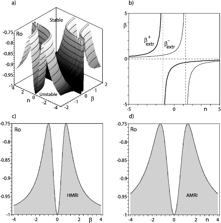
Figure 1: (a) The function ${\rm Ro}^{-}(\beta,n)$ given by Eq. (101) at ${\rm Rb=-25/32}$. (b) Its extremizers (104) along which the critical hydrodynamic Rossby number attains the maximal value ${\rm Ro}^{-}=-3/4$ . The cross-section of the function at (c) $n=0$ (HMRI) and (d) at $\beta\rightarrow+\infty$ (AMRI).

8.2 Extremal properties of the critical hydrodynamic Rossby number

For a given magnetic Rossby number, $\rm Rb$, the functions ${\rm Ro}^{\pm}(n,\beta)$ take their extrema

$${\rm Ro}_{\rm extr}^{\pm}=-2-4{\rm Rb}\pm 2\sqrt{2{\rm Rb}(2{\rm Rb}+1)}$$ (103)

at the following extremal curves in the $(n,\beta)$-plane (cf. Kirillov et al. (2012))

$$\beta_{\rm extr}^{+}=\frac{-1}{n+\sqrt{-2{\rm Rb}}},\quad\beta_{\rm extr}^{-}=\frac{-1}{n-\sqrt{-2{\rm Rb}}},$$ (104)

see Fig. 1(b). The branch ${\rm Ro}^{-}(\beta,n)$ is shown in Fig. 1(a) for ${\rm Rb}=-25/32$ (this particular value has been chosen since it is the minimum value which leads to destabilization of Keplerian profiles, as we will see below). The maximal value of the hydrodynamic Rossby number is constant along the curves (104), see Fig. 1(a,b).

The cross-section of the function ${\rm Ro}^{-}(\beta,n)$ at $n=0$ corresponding to the helical magnetorotational instability (HMRI) is plotted in Fig. 1(c). In contrast, Fig. 1(d) shows the limit $\beta\rightarrow+\infty$

$${\rm Ro}^{-}(n,{\rm Rb})=-2+(n^{2}-2{\rm Rb})\frac{n^{2}-2{\rm Rb}-\sqrt{(n^{2}-2{\rm Rb})^{2}-4n^{2}}}{2n^{2}}$$ (105)

corresponding to the azimuthal magnetorotational instability (AMRI).

The function (105) attains its maximal value ${\rm Ro}_{\rm extr}^{-}$ given by equation (103) at

$$n=\pm\sqrt{-2{\rm Rb}}.$$ (106)

Since by definition (93) $n=\frac{m}{\alpha}$ where $\frac{k_{z}}{\sqrt{k_{R}^{2}+k_{z}^{2}}}=:\alpha\in[0,1]$, then for ${\rm Rb}\in[-1,-0.5]$ the condition (106) yields the only possible integer values of the azimuthal wavenumber:

$$m=\pm 1.$$

This means that the effect of the purely azimuthal magnetic field is most pronounced at the maximal possible range of variation of the hydrodynamic Rossby number for the lowest azimuthal modes with $m=\pm 1$ (Hollerbach et al., 2010; Kirillov et al., 2014).

8.3 A band structure periodic in $\alpha$

What is the general dependence of the mode number $m$ on $\alpha$, $\rm Rb$, and the ratio $\omega_{A_{\phi}}/\omega_{A_{z}}$ of the azimuthal to the axial magnetic fields? Let us express $\alpha$ from the Eq. (104) as

$$\alpha=\pm\left(m+\frac{\omega_{A_{z}}}{\omega_{A_{\phi}}}\right)\frac{1}{\sqrt{-2{\rm Rb}}}.$$ (107)

The ratio $\omega_{A_{\phi}}/\omega_{A_{z}}$ being plotted against $\alpha$ at different $m$ and $\rm Rb$ uncovers a regular pattern shown in Fig. 2. The pattern is periodic in $\alpha$ with the period $1/\sqrt{-2{\rm Rb}}$. On the other hand, the dependence of $\alpha$ on the ratio of the magnetic fields is a continuous piecewise smooth function inside every vertical ‘band’ with the width $1/(2\sqrt{-2{\rm Rb}})$ in $\alpha$, see Fig. 2(b). The vertical bands in Fig. 2 are further separated into the cells with the boundaries at

$$\frac{\omega_{A_{\phi}}}{\omega_{A_{z}}}=\frac{2}{1},\frac{2}{2},\frac{2}{3},\frac{2}{4},\frac{2}{5},\frac{2}{6},\ldots.$$ (108)

Every particular cell in Fig. 2 corresponds to a unique integer azimuthal wavenumber $m$. Note however that the cells with the same $m$ are grouped along the same hyperbolic curve given by equation (107).

Figure 2: The periodic in $\alpha$ band structure at (a) ${\rm Rb}=-1$ (with gray cells corresponding to $m=-2$) and (b) ${\rm Rb}=-0.5$ (with the gray stripe marking the first band).

The curves (107) with the slopes of the same sign do not cross. The crossings of two hyperbolic curves (107) with the integer indices $m_{1}$ and $m_{2}$ and slopes of different sign happen at

$$\alpha=\frac{m_{1}-m_{2}}{2\sqrt{-2{\rm Rb}}},\quad{\rm and}\quad\frac{\omega_{A_{\phi}}}{\omega_{A_{z}}}=\frac{-2}{m_{1}+m_{2}},$$ (109)

which explains the sequence (108). Within one and the same band with $\alpha\geq 0$ the cells are encoded by the two interlacing series of integers, e.g. for the third band in Fig. 2(a)

$$m=+1,-2,0,-3,-1,-4,-2,-5,-3,-6,\ldots,$$ (110)

which is a mixture of the sequences

$$+1,0,-1,-2,-3,\ldots\quad{\rm and}\quad-2,-3,-4,-5,-6,\ldots,$$

whereas for the second band with $\alpha\geq 0$ in Fig. 2(a) we have

$$m=-1,0,-2,-1,-3,-2,-4,-3,-5,-4,\ldots,$$ (111)

which corresponds to the two interlacing sequences

$$-1,-2,-3,-4,-5,\ldots\quad{\rm and}\quad 0,-1,-2,-3,-4,\ldots.$$ (112)

Therefore, at the crossings (109) with $\alpha\neq 0$ the quadruplet of cells consists of two pairs; each pair corresponding to a different value of the azimuthal wavenumber $m$. At the crossings with $\alpha=0$ all the four cells in the quadruplet have the same $m$.

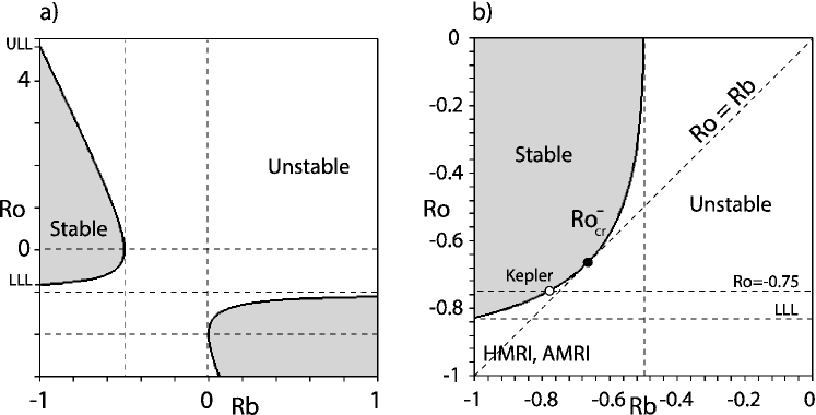
Figure 3: (a) The lower (LLL) and the upper (ULL) Liu limits existing at ${\rm Rb}=-1$ are points on the quasi-hyperbolic curve (115) in the ${\rm Ro}-{\rm Rb}$ plane. (b) A scaled fragment of the limiting curve (114) demonstrating that the inductionless forms of the magnetorotational instability exist above the lower Liu limit ${\rm Ro}_{\rm extr}^{-}=2-2\sqrt{2}$ when ${\rm Rb}>-25/32$. The open circle marks the Keplerian value for the Rossby number ${\rm Ro}=-3/4$ at ${\rm Rb}=-25/32$ whereas the black circle corresponds to ${\rm Ro}={\rm Rb}=-2/3$. The dashed diagonal is given by the equation ${\rm Ro}={\rm Rb}$.

8.4 Continuation of the Liu limits to arbitrary $\rm Rb$

The extrema (103) can be represented in the form

$${\rm Ro}_{\rm extr}^{\pm}=-1-(\sqrt{2{\rm Rb}}\mp\sqrt{1+2{\rm Rb}})^{2},$$ (113)

which is equivalent to the expression

$${\rm Rb}=-\frac{1}{8}\frac{({\rm Ro}+2)^{2}}{{\rm Ro}+1}$$ (114)

that is universal in the sense that it contains only logarithmic derivatives of the radial profiles of the flow and the azimuthal field.

The particular case of equation (114) at ${\rm Rb}=-1$ yields the result of Liu et al. (2006), reproduced also by Kirillov & Stefani (2011) and Priede (2011). Solving (114) at ${\rm Rb}=-1$, we find that the critical Rossby numbers ${\rm Ro}({\rm Ha},{\rm Re},n,\beta)$ given by the equation (99) and thus the instability domains lie at ${\rm Pm}=0$ and ${\rm Rb}=-1$ outside the stratum

$$2-2\sqrt{2}=:{\rm Ro}_{\rm LLL}<{\rm Ro}({\rm Ha},{\rm Re},n,\beta)<{\rm Ro}_{\rm ULL}:=2+2\sqrt{2},$$

where ${\rm Ro}_{\rm LLL}$ is the value of ${\rm Ro}^{-}_{\rm extr}$ at the lower Liu limit (LLL) and ${\rm Ro}_{\rm ULL}$ is the value of ${\rm Ro}^{+}_{\rm extr}$ at the upper Liu limit (ULL) corresponding to the critical values of $\beta$ given by the equation (104).

Fig. 3(a) shows how the LLL and ULL continue to the values of ${\rm Rb}\neq-1$. In fact, the LLL and the ULL are points at the quasi-hyperbolic curve

$$({\rm Rb}-{\rm Ro}-1)^{2}-({\rm Rb}+{\rm Ro}+1)^{2}=\frac{1}{2}({\rm Ro}+2)^{2},$$ (115)

which is another representation of equation (114). At ${\rm Rb}=-1/2$ the branches ${\rm Ro}_{\rm extr}^{-}({\rm Rb})$ and ${\rm Ro}_{\rm extr}^{+}({\rm Rb})$ meet each other. Therefore, the inductionless magnetorotational instability at negative $\rm Rb$ exists also at positive $\rm Ro$ when ${\rm Ro}>{\rm Ro}_{\rm extr}^{+}({\rm Rb})$, Fig. 3(a). Notice also the second stability domain at ${\rm Rb}>0$ and ${\rm Ro}<-1$.

We see that in the inductionless case ${\rm Pm}=0$ when the Reynolds and Hartmann numbers subsequently tend to infinity as described in Section 8.1 and $\beta$ and $n$ are under the constraints (104), the maximal possible critical Rossby number ${\rm Ro}_{\rm extr}^{-}$ increases with the increase of ${\rm Rb}$. At

$${\rm Rb}\geq-\frac{25}{32}=-0.78125$$ (116)

${\rm Ro}_{\rm extr}^{-}({\rm Rb})$ exceeds the critical value for the Keplerian flow: ${\rm Ro}_{\rm extr}^{-}\geq-3/4$.

Therefore, the possibility for $B_{\phi}(R)$ to depart from the profile $B_{\phi}(R)\propto R^{-1}$ allows us to break the conventional lower Liu limit and extend the inductionless versions of MRI to the velocity profiles $\Omega(R)$ as flat as the Keplerian one and even to less steep profiles, including that of the solid body rotation, i.e. ${\rm Ro=0}$, for ${\rm Rb}\geq-1/2$, Fig. 3(b).

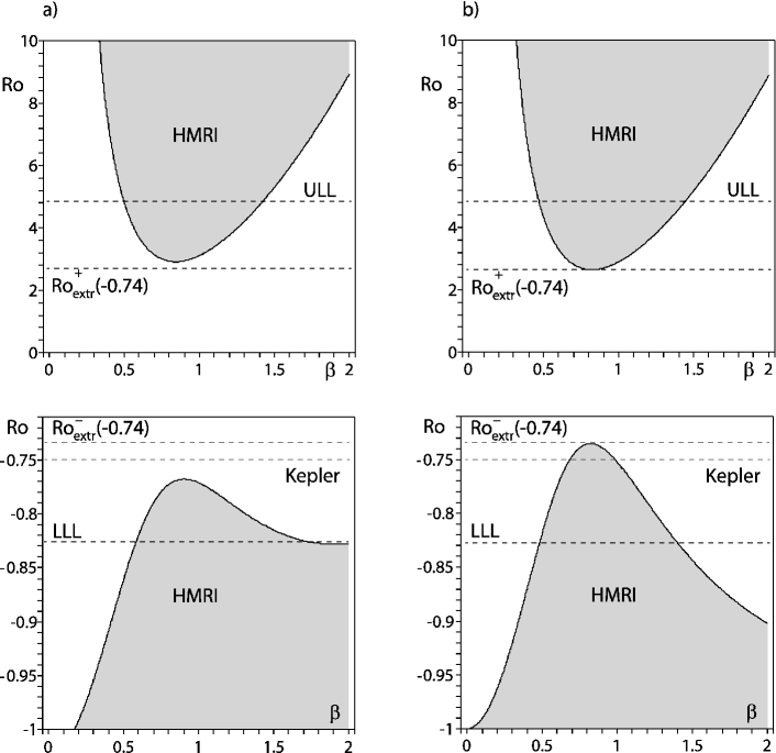
Figure 4: Domains of the inductionless HMRI for $\rm Pm=0$, $n=0$, and $\rm Rb=-0.74$ when the Hartmann and Reynolds numbers follow the scaling law (117) with $\beta$ satisfying the restraints (104): (a) ${\rm Ha}=5$ and ${\rm Re}\approx 92$; (b) ${\rm Ha}=100$ and ${\rm Re}\approx 736158$. With the increase in $\rm Ha$ and $\rm Re$ the HMRI domain easily breaks the conventional Liu limits as well as the Kepler line $\rm Ro=-0.75$ and its boundary tends to the curves (101) that touch the new limits for the critical Rossby number: ${\rm Ro}^{-}_{\rm extr}(-0.74)\approx-0.726$ and ${\rm Ro}^{+}_{\rm extr}(-0.74)\approx 2.646$.

8.5 Scaling law of the inductionless MRI

What asymptotic behavior of the Reynolds and Hartmann numbers at infinity leads to maximization of negative (and simultaneously to minimization of positive) critical Rossby numbers? To get an idea, we investigate extrema of $\rm Ro$ as a solution to equation (99) subject to the constraints (104). Taking, e.g., $\beta=\beta_{\rm extr}^{-}$ in equation (99), differentiating the result with respect to $\rm Ha$, equating it to zero and solving the equation for $\rm Re$, we find the following asymptotic relation between $\rm Ha$ and $\rm Re$ when ${\rm Ha}\rightarrow\infty$:

$${\rm Re}=2{\rm Rb}\sqrt{3{\rm Rb}+2}(\sqrt{1+2{\rm Rb}}+\sqrt{2{\rm Rb}})\beta^{3}{\rm Ha}^{3}+O({\rm Ha}).$$ (117)

For example, at ${\rm Rb}=-1$ and $n=0$ we have $\beta=\beta_{\rm extr}^{-}=1/\sqrt{2}$. After taking this into account in (117) we obtain the scaling law of HMRI found in Kirillov & Stefani (2010)

$${\rm Re}=\frac{2+\sqrt{2}}{2}{\rm Ha}^{3}+O({\rm Ha}).$$ (118)

Figure 4 shows the domains of the inductionless helical MRI at ${\rm Rb}=-0.74$ when the Hartmann and the Reynolds numbers are increasing in accordance with the scaling law (117). The instability thresholds easily penetrate the LLL and ULL as well as the Keplerian line and tend to the curves (101) that touch the new limits for the critical Rossby number: ${\rm Ro}^{-}_{\rm extr}(-0.74)\approx-0.726$ and ${\rm Ro}^{+}_{\rm extr}(-0.74)\approx 2.646$. Note that the curves (101) correspond also to the limit of vanishing Elsasser number $\rm N$, because according to the scaling law (117) we have ${\rm N}\propto 1/{\rm Ha}$ as ${\rm Ha}\rightarrow\infty$. This observation makes the dispersion relation (97) advantageous for investigation of the inductionless versions of MRI.

8.6 Growth rates of HMRI and AMRI and the critical Reynolds number

We will calculate the growth rates of the inductionless MRI with the use of the dispersion relation (97). Assuming in (97) ${\rm Rm}:={\rm Re}{\rm Pm}=0$, we find the roots explicitly:

$$\lambda_{1,2}=-in+{\rm N}\left(2\beta^{2}{\rm Rb}-(n\beta+1)^{2}\right)-\frac{1}{\rm Re}\pm 2\sqrt{X+iY},$$ (119)

where

$$X={\rm N}^{2}\beta^{2}\left(\beta^{2}{\rm Rb}^{2}+(n\beta+1)^{2}\right)-{\rm Ro}-1,\quad Y={\rm N}\beta({\rm Ro}+2)(n\beta+1).$$ (120)

Separating the real and imaginary parts of the roots, we find the growth rates of the inductionless MRI in the closed form:

$$(\lambda_{1,2})_{r}={\rm N}\left(2\beta^{2}{\rm Rb}-(n\beta+1)^{2}\right)-\frac{1}{\rm Re}\pm\sqrt{2X+2\sqrt{X^{2}+Y^{2}}}.$$ (121)

Particularly, at $n=0$ we obtain the growth rates of the axisymmetric helical magnetorotational instability in the inductionless case.

Introducing the Elsasser number of the azimuthal field as

$${\rm N}_{A}:=\beta^{2}{\rm N}$$ (122)

and then taking the limit of $\beta\rightarrow\infty$ we obtain from the equation (121) the growth rates of the inductionless azimuthal MRI:

$$(\lambda_{1,2})_{r}={\rm N}_{A}(2{\rm Rb}-n^{2})-\frac{1}{\rm Re}\pm\sqrt{2}$$ (123)

$$\times\sqrt{{\rm N}_{A}^{2}({\rm Rb}^{2}+n^{2})-{\rm Ro}-1+\sqrt{\left({\rm N}_{A}^{2}({\rm Rb}^{2}+n^{2})-{\rm Ro}-1\right)^{2}+{\rm N}_{A}^{2}({\rm Ro}+2)^{2}n^{2}}}.$$

In the inviscid limit ${\rm Re}\rightarrow\infty$ the term $\frac{1}{\rm Re}$ vanishes in the expressions (121) and (123).

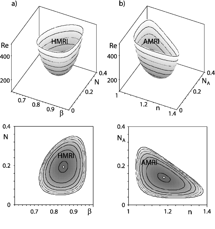
Figure 5: Domain of the viscous inductionless MRI (124) of a Keplerian flow ($\rm Ro=-0.75$) at $\rm Rb=-0.75$ when (a) $n=0$ (axisymmetric HMRI) and (b) $\beta\rightarrow\infty$ (nonaxisymmetric AMRI). Open circles mark the location of the minima of the critical hydrodynamic Reynolds number: (a) $\beta\approx 0.848$, ${\rm N}\approx 0.193$, ${\rm Re}\approx 198.5$; (b) $n\approx 1.180$, ${\rm N}_{A}\approx 0.139$, ${\rm Re}\approx 198.5$.

On the other hand, in the viscous case the condition $(\lambda_{1,2})_{r}>0$ yields the critical hydrodynamic Reynolds number beyond which inductionless MRI appears. For example, from the equation (121) we find the following criterion for the onset of the instability:

$${\rm Re}>\frac{1}{{\rm N}\left(2\beta^{2}{\rm Rb}-(n\beta+1)^{2}\right)+\sqrt{2X+2\sqrt{X^{2}+Y^{2}}}}.$$ (124)

With $n=0$ the criterion (124) corresponds to the axisymmetric HMRI. A similar criterion for the onset of AMRI follows from the expression (123).

The critical hydrodynamic Reynolds number for a Keplerian flow at ${\rm Rb}=-0.75$ is plotted in Fig. 5 as a function of the Elsasser number and (Fig. 5(a)) $\beta$ in case of the axisymmetric HMRI and (Fig. 5(b)) $n$ in case of the non-axisymmetric AMRI. In both cases the minimal $\rm Re$ at the onset of instability is about $200$.

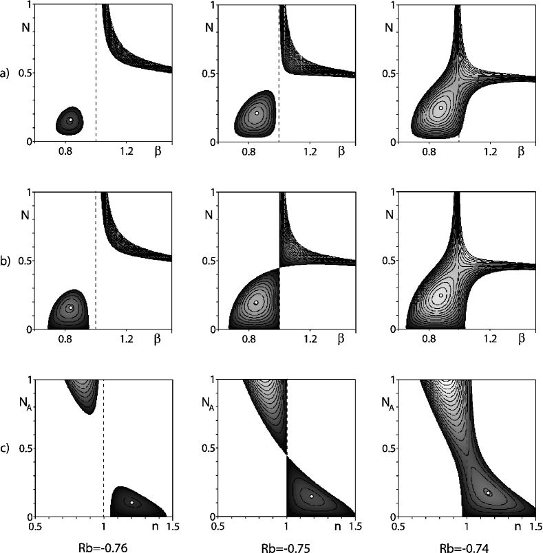
Figure 6: $\rm Ro=-0.75$. Row (a): The growth rates $\lambda_{r}\geq 0$ of viscous (${\rm Re}=800$) HMRI ($n=0$) in the inductionless $(\rm Pm=0)$ limit in projection onto the ${\rm N}-\beta$ plane. Row (b): The same in the inviscid $({\rm Re}\rightarrow\infty)$ limit. Row (c): The growth rates $\lambda_{r}\geq 0$ of AMRI ($\beta\rightarrow\infty$) in the inductionless and inviscid limit in projection onto the ${\rm N}_{A}-n$ plane. The open circles mark the maxima of $\lambda_{r}$. Row (a): $\beta\approx 0.830$, ${\rm N}\approx 0.153$, $\lambda_{r}\approx 0.002$; $\beta\approx 0.848$, ${\rm N}\approx 0.193$, $\lambda_{r}\approx 0.004$; $\beta\approx 0.869$, ${\rm N}\approx 0.236$, $\lambda_{r}\approx 0.007$. Row (b): $\beta\approx 0.830$, ${\rm N}\approx 0.153$, $\lambda_{r}\approx 0.003$; $\beta\approx 0.848$, ${\rm N}\approx 0.193$, $\lambda_{r}\approx 0.005$; $\beta\approx 0.869$, ${\rm N}\approx 0.236$, $\lambda_{r}\approx 0.008$; Row (c): $n\approx 1.204$, ${\rm N}_{A}\approx 0.105$, $\lambda_{r}\approx 0.003$; $n\approx 1.180$, ${\rm N}_{A}\approx 0.139$, $\lambda_{r}\approx 0.005$; $n\approx 1.151$, ${\rm N}_{A}\approx 0.178$, $\lambda_{r}\approx 0.008$.

8.7 HMRI and AMRI as magnetically destabilized inertial waves

Consider the Taylor expansion of the eigenvalues (119) with respect to the Elsasser number ${\rm N}$ in the vicinity of ${\rm N}=0$

$$\lambda_{1,2}=-i(n\mp 2\sqrt{{\rm Ro}+1})-\frac{1}{\rm Re}$$

$$+{\rm N}\left(-(n\beta+1)^{2}+2\beta^{2}{\rm Rb}\pm\beta\frac{({\rm Ro}+2)}{\sqrt{{\rm Ro}+1}}(n\beta+1)\right)+O({\rm N}^{2}).$$ (125)

Expressions (119) and (8.7) generalize the result of Priede (2011) to the case of arbitrary $n$, ${\rm Re}$, and $\rm Rb$ and exactly coincide with it at $n=0$, ${\rm Re}\rightarrow\infty$, and ${\rm Rb}=-1$.

In the absence of the magnetic field (${\rm N}=0$) the eigenvalues $\lambda_{1,2}$ correspond to damped inertial (or Kelvin) waves. According to (124) at finite ${\rm Re}$ there exists a critical finite ${\rm N}>0$ that is necessary to trigger destabilization of the inertial waves by the magnetic field, see Fig. 5 and Fig. 6(a). However, as the expansion (8.7) demonstrates, in the limit ${\rm Re}\rightarrow\infty$ the inductionless magnetorotational instability occurs when the effect of the magnetic field is much weaker than that of the flow — even when the Elsasser number is infinitesimally small, Fig. 6(b,c).

In the inviscid case the boundary of the domain of instability (124) takes the form

$${\rm N}=\pm 2\sqrt{\frac{\beta^{2}({\rm Ro}+2)^{2}(n\beta+1)^{2}-((n\beta+1)^{2}-2\beta^{2}{\rm Rb})^{2}({\rm Ro}+1)}{((n\beta+1)^{2}-4\beta^{2}({\rm Rb}+1))((n\beta+1)^{2}-2\beta^{2}{\rm Rb})^{2}(n\beta+1)^{2}}}.$$ (126)

The lines (126) bound the domain of non-negative growth rates of HMRI in Fig. 6(b).

When ${\rm Ro}={\rm Rb}$, the stability boundary (126) has a self-intersection at

$$n=-\frac{1}{\beta}\pm 2\sqrt{{\rm Rb}+1},\quad{\rm N}=\frac{\pm 1}{2\beta^{2}}\sqrt{\frac{-(3{\rm Rb}+2)}{({\rm Rb}+1)({\rm Rb}+2)}}.$$ (127)

For example, when ${\rm Rb}={\rm Ro}=-0.75$ and $n=0$, the intersection happens at $\beta=1$ and ${\rm N}=\sqrt{5}/5$, Fig. 6(b). If ${\rm Rb}={\rm Ro}=-0.75$ and $\beta\rightarrow\infty$, the intersection point is at $n=1$ and ${\rm N}_{A}=\sqrt{5}/5$, Fig. 6(c). In general, the intersection exists at ${\rm N}\neq 0$ for

$${\rm Ro}={\rm Rb}<-\frac{2}{3}.$$ (128)

At ${\rm Ro}={\rm Rb}=-\frac{2}{3}$ the intersection occurs at ${\rm N}=0$.

In Fig. (6) we see that when ${\rm Ro}<-\frac{2}{3}$ and ${\rm Ro}>{\rm Rb}$, the instability domain consists of two separate regions. In the case when ${\rm Ro}<-\frac{2}{3}$ and ${\rm Ro}<{\rm Rb}$, the two regions merge into one. When the condition (128) is fulfilled, the two sub-domains touch each other at the point (127). At ${\rm Ro}={\rm Rb}=-\frac{2}{3}$ the lower region shrinks to a single point which simultaneously is the intersection point (127) with ${\rm N}=0$.

On the other hand, given ${\rm Ro}<-2/3$ and decreasing ${\rm Rb}$ we find that the single instability domain tends to split into two independent regions after crossing the line ${\rm Ro}={\rm Rb}$. The further decrease in ${\rm Rb}$ yields diminishing the size of the lower instability region, see Fig. 6. At which ${\rm Rb}$ does the lower instability region completely disappear?

Clearly, the lower region disappears when the roots of the equation ${\rm N}(n)=0$ become complex. From the expression (126) we derive

$$(n\beta+1)^{2}\pm\beta\frac{{\rm Ro}+2}{\sqrt{{\rm Ro}+1}}(n\beta+1)-2\beta^{2}{\rm Rb}=0.$$ (129)

The equations (129) have the roots $n$ complex if and only if their discriminant is negative:

$$\frac{({\rm Ro}+2)^{2}}{{\rm Ro}+1}+8{\rm Rb}<0,$$ (130)

which is simply the domain with the boundary given by the curve connecting the two Liu limits (114) that is shown in Fig. 3. Note that ${\rm Rb}=-2/3$ and ${\rm Ro}=-2/3$ satisfy the equation (114), which indicates that the line ${\rm Ro}={\rm Rb}$ is tangent to the curve (114) at the point $(-2/3,-2/3)$ in the ${\rm Ro}$-${\rm Rb}$ plane, see Fig. 3(b).

Finally, we notice that the left side of the equation (129) is precisely the coefficient at $\rm N$ in the expansion (8.7). In the inviscid case it determines the limit of the stability boundary as ${\rm N}\rightarrow 0$, quite in accordance with the scaling law (117). Solving the equation (129) for ${\rm Ro}$, we exactly reproduce the formula (101). At $n=0$ and ${\rm Rb}=-1$ the equation (129) exactly coincides with that obtained by Priede (2011).

9 HMRI and AMRI at very small, but finite $\rm Pm$

An advantage of the inductionless limit discussed above is the considerable simplification of dispersion relations at $\rm Pm=0$ or $\rm Rm=0$ that yields expressions for growth rates and stability criteria in explicit and closed form. There are, however, real physical situations that are characterized by small but finite values of the magnetic Reynolds and Prandtl numbers. Below, we demonstrate numerically that HMRI and AMRI exist also when $\rm Pm\neq 0$ or $\rm Rm\neq 0$. The pattern of the stability domains keeps the structure that we have found in the inductionless case. Moreover, the instability criteria of the inductionless limit serve as rather accurate guides in the physically more realistic situation of finite, but very small, $\rm Pm$.

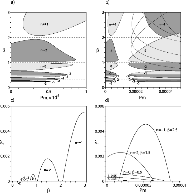
Figure 7: $\rm Ha=30$, $\rm Ro=-0.75$, $\rm Re=40000$, $\rm Rb=-0.755$. (a,b) Islands of low $\rm Pm$ magnetorotational instability (axisymmetric HMRI with $n=0$, non-axisymmetric HMRI with $n\neq 0,+1$ at $\beta\leq 2$ and AMRI with $n=+1$ at $\beta>2$) corresponding to different modified azimuthal wave numbers $n$. (c,d) The growth rates $\lambda_{r}$ of the perturbation (c) as functions of $\beta$ at ${\rm Pm}=4\cdot 10^{-6}$ and different $n$ and (d) as functions of $\rm Pm$ at different $n$ and $\beta$.

9.1 Islands of HMRI at various integer $n$ and their reconnection

Consider the dispersion relation (94) and substitute its coefficients (B) into the Bilharz matrix (82). Applying the Bilharz criterion (83) to the result, we find that it is the condition of vanishing the determinant of the Bilharz matrix that determines the instability threshold. Fixing the Rossby number at the Keplerian value $\rm Ro=-0.75$ and assuming some reasonable values for the Hartmann and Reynolds numbers, e.g. $\rm Ha=30$ and $\rm Re=40000$, we choose the magnetic Rossby number slightly to the right of the line ${\rm Ro}={\rm Rb}$, which according to the criterion (116) should result in instability, at least in the inductionless case. For various integer modified azimuthal wavenumbers $n$ we plot the instability domains in the $\beta-{\rm Pm}$ plane, Fig. 7(a,b).

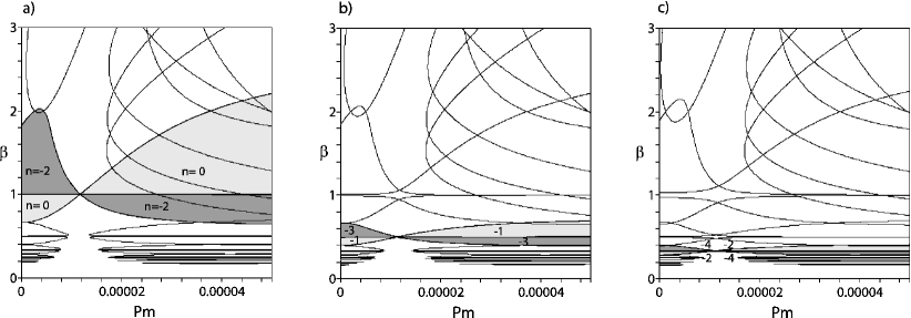
Figure 8: Subsequently reconnecting instability islands at $\rm Ha=30$, $\rm Ro=-0.75$, $\rm Re=40000$ and growing ${\rm Rb}>-0.75$: (a) $\rm Rb=-0.74933$, (b) $\rm Rb=-0.747$, and (c) $\rm Rb=-0.742$.

We see that at every integer $n$ there are several instability islands (curiously resembling those originating in a pure hydrodynamical Taylor-Couette problem (Altmeyer et al., 2011)). As is visible in Fig. 7(b) they tend to group into two clusters.

The first cluster consists of the islands situated at ${\rm Pm}<10^{-5}$ and contains intervals of the positive $\beta$-axis at all $n$ but $n=+1$, Fig. 7(a). Note that the modified azimuthal wavenumber $n$ corresponding to these islands follows exactly the sequence (110) that we have found in the inductionless case! The growth rates, i.e. the real parts of the roots $\lambda$ defined via relations (96), are plotted in Fig. 7(c) for a fixed value of $\rm Pm$ that cuts this cluster along a vertical line. Fig. 7(d) demonstrates the growth rates at various $\beta$ corresponding to particular values of $n$. We see that for all $n$ but $n=+1$ the growth rates tend to some positive values as ${\rm Pm}\rightarrow 0$ indicating a smooth transition to the inductionless magnetorotational instabilities that occur both for axisymmetric ($n=0$) and non-axisymmetric ($n\neq 0$) perturbations. This seems to be the main reason for the manifestation of the sequence (110) in the pattern of the instability islands of Fig. 7(c).

The second cluster of the instability islands occupies the region at ${\rm Pm}>10^{-5}$ and is encoded by the sequence (111), see Fig. 7(b). We see that the islands of the two clusters tend to form quadruplets. Each quadruplet consists of the two pairs of islands corresponding to the indices $n$ that differ by $2$, for example: $0$ and $-2$, $-1$ and $-3$, $-2$ and $-4$ etc. Each quadruplet whose pairs are labeled with the indices $n_{i},n_{j}\leq 0$ tends to be centered at $\beta=\beta_{ij}$, where

$$\beta_{ij}=-\frac{2}{n_{i}+n_{j}},$$ (131)

which is exactly the second of the equations (109). Moreover, the whole pattern of the instability islands in Fig. 7(b) repeats the pattern of cells in the second and third bands shown in Fig. 2(a).

It is natural to ask what are the conditions for reconnection of the islands in the pairs that constitute every particular quadruplet. To get an idea we play with the two Rossby numbers in Fig. 8. We fix ${\rm Ro}=-0.75$ and slightly increase $\rm Rb$. As a result, at ${\rm Rb}=-0.74933$ the islands with the indices $n=-2$ and $n=0$ reconnect at $\beta_{-2,0}=1$, Fig. 8(a). At ${\rm Rb}=-0.747$ these islands overlap whereas the islands in the next quadruplet with $n=-3$ and $n=-1$ reconnect at $\beta_{-3,-1}=-1/2$, Fig. 8(b). At $\rm Rb=-0.742$ the reconnection happens in the third quadruplet at $\beta_{-4,-2}=1/3$, and so on, Fig. 8(c).

This sequence of the reconnections indicates the special role of the line ${\rm Ro}={\rm Rb}$ which seems to be even more pronounced in the inviscid limit $({\rm Re}\rightarrow\infty)$. In the following we check these hypotheses when the magnetic field has only the azimuthal component which corresponds to the limit $\beta\rightarrow\infty$.

9.2 AMRI as a dissipation-induced instability of Chandrasekhar’s equipartition solution

In the matrix (98) let us replace via the relation (122) the Elsasser number $\rm N$ of the axial field with the Elsasser number of the azimuthal field ${\rm N}_{A}$ and then let $\beta\rightarrow\infty$. If, additionally

$${\rm N}_{A}={\rm Rm}$$ (132)

and

$$\rm Ro=Rb,$$ (133)

then in the ideal limit ($\rm Re\rightarrow\infty$, $\rm Rm\rightarrow\infty$) the roots of the dispersion relation (97) are

$$\lambda_{1,2}=0,\quad\lambda_{3,4}=-2i(n\pm 1).$$ (134)

Figure 9: (a) The threshold of instability (9.2) at ${\rm N}_{A}={\rm Rm}$ and $\rm Re\rightarrow\infty$ in the $(n,{\rm Rb},{\rm Rm})$ space and (b) its projection onto ${\rm Rb}-n$ plane. The increase in $\rm Rm$ makes the instability domain more narrow so that in the limit ${\rm Rm}\rightarrow\infty$ it degenerates into a ray (dashed) on the straight line (136) that emerges from the point (open circle) with the coordinates $n=\frac{2\sqrt{3}}{3}$ and ${\rm Rb}=-\frac{2}{3}$ and passes through the point with $n=1$ and ${\rm Rb}=-1$.

With the use of the relations (93) it is straightforward to verify that the condition (132) requires that $\Omega=\omega_{A_{\phi}}$. Thus, the conditions (132) and (133) are equivalent to (91), which at ${\rm Rb}={\rm Ro}=-1$ define the Chandrasekhar equipartition solution (Kirillov et al., 2014) belonging to a wide class of exact stationary solutions of MHD equations for the case of ideal incompressible infinitely conducting fluid with total constant pressure that includes even knotted flows (Golovin & Krutikov, 2012). It is well-known that the Chandrasekhar equipartition solution is marginally stable (Chandrasekhar, 1956, 1961; Bogoyavlenskij, 2004). According to equation (134) the marginal stability is preserved in the ideal case also when ${\rm Rb}={\rm Ro}\neq-1$. Will the roots (134) acquire only negative real parts with the addition of electrical resistivity?

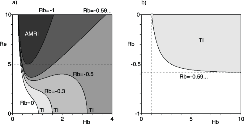
Figure 10: At $n\approx 1.27842$ (a) The domain of the inductionless azimuthal MRI bounded by the curve (140) with $\rm Ro=-1$ and $\rm Rb=-1$ that gradually transforms into the domain that includes the Tayler instability (TI) as $\rm Rb$ increases from $-1$ to $0$; (b) Tayler instability corresponding to $\rm Ro=0$ and $\rm Re=0$. The open circle marks the onset of the standard TI at $\rm Rb=0$ with the critical ${\rm Hb}\approx 1.04117$.

In general, the answer is no. Indeed, under the constraints (132) and (133) in the limit of vanishing viscosity ($\rm Re\rightarrow\infty$) the Bilharz criterion applied to the dispersion relation (97) gives the following threshold of instability:

$$16(n^{2}-{\rm Rb}^{2})(n^{2}-{\rm Rb}-2)^{2}{\rm Rm}^{4}$$

$$+(n^{6}-12n^{2}{\rm Rb}^{2}+32n^{2}({\rm Rb}+1)-16{\rm Rb}^{2}({\rm Rb}+2)){\rm Rm}^{2}$$

$$-4{\rm Rb}^{2}+4n^{2}({\rm Rb}+1)=0.$$ (135)

In the $(n,{\rm Rb},{\rm Rm})$ space the domain of instability is below the surface specified by equation (9.2), see Fig. 9(a). When the electrical resistivity is vanishing, the cross-sections of the instability domain in the ${\rm Rb}-n$ plane become smaller and in the limit ${\rm Rm}\rightarrow\infty$ they tend to the ray on the line

$${\rm Rb}=-\frac{2}{3}+\frac{n\sqrt{3}-2}{3(2-\sqrt{3})}$$ (136)

that starts at the point with the coordinates $n=\frac{2\sqrt{3}}{3}$ and ${\rm Rb}=-\frac{2}{3}$ and passes through the point with $n=1$ and ${\rm Rb}=-1$, Fig. 9(b). For example, at $\rm Ro=Rb=-\frac{3}{4}$ the equation (136) yields

$$n=\frac{1}{4}+\frac{\sqrt{3}}{2}.$$ (137)

On the contrary, when the magnetic Reynolds number ${\rm Rm}$ decreases, the instability domain widens up and in the inductionless limit at $\rm Rm=0$ it is bounded by the curve

$${\rm Rb}=\frac{n(n-\sqrt{n^{2}+4})}{2}.$$ (138)

The wide part of the instability domain shown in Fig. 9(a) that exists at small $\rm Rm$ belongs to the realm of the azimuthal magnetorotational instability (AMRI). We see that this instability quickly disappears with the increase of $\rm Rm$ or $\rm Rb$. On the other hand, the ideal solution with the roots (134) that corresponds to the limit ${\rm Rm}\rightarrow\infty$ is destabilized by the electrical resistivity. For $n$ given by equation (137) we have, for example, an unstable root $\lambda\approx 0.00026-i0.00493$ at $\rm Rm=100$. In general, if $\rm Rb$ and $n$ satisfy (136), then already an infinitesimally weak electrical resistivity destabilizes the solution specified by the constraints (132) and (133) at vanishing kinematic viscosity that includes Chandrasekhar’s equipartition solution as a special case. This dissipation-induced instability (Kirillov, 2009; Kirillov & Verhulst, 2010; Kirillov, 2013) further develops into the AMRI with ${\rm Rm}$ decreasing to zero.

10 Transition from AMRI to the Tayler instability

The Tayler instability (Tayler, 1973; Rüdiger & Schultz, 2010) is a current-driven, kink-type instability that taps into the magnetic field energy of the electrical current in the fluid. Although its plasma-physics counterpart has been known for a long time, its occurrence in a liquid metal was observed only recently (Seilmayer et al., 2012). In the context of the on-going liquid-metal experiments in the frames of the DRESDYN project (Stefani et al., 2012) it is interesting to get an insight on the transition between the azimuthal magnetorotational instability and the Tayler instability.

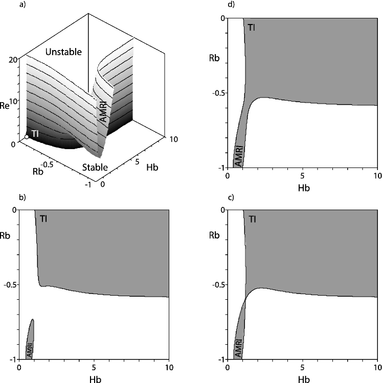
Figure 11: Under the assumption that ${\rm Ro}({\rm Rb})=-\sqrt{-\rm Rb^{2}-2\rm Rb}$ and $n\approx 1.27842$ (a) The domain of the inductionless instability bounded by the surface (140) in the $({\rm Hb},{\rm Rb},{\rm Re})$ space and its cross-sections at (b) $\rm Re=5.4$, (c) $\rm Re=5.734$, and (d) $\rm Re=6$. The domains of TI and AMRI reconnect via a saddle point at $\rm Re=5.734$.

Consider the instability threshold (99) obtained in the inductionless approximation (${\rm Pm}=0$). Let us introduce the Hartmann number corresponding to the pure azimuthal magnetic field as

$${\rm Hb}:=\beta{\rm Ha},$$ (139)

so that ${\rm N}_{A}=\frac{{\rm Hb}^{2}}{\rm Re}$. Substituting (139) into (99) and then letting $\beta\rightarrow\infty$, we find

$${\rm Re}^{2}=\frac{((1+{\rm Hb}^{2}n^{2})^{2}-4{\rm Hb}^{2}{\rm Rb}(1+{\rm Hb}^{2}n^{2})-4{\rm Hb}^{4}n^{2})(1+{\rm Hb}^{2}(n^{2}-2{\rm Rb}))^{2}}{4({\rm Hb}^{4}{\rm Ro}^{2}n^{2}-((1+{\rm Hb}^{2}(n^{2}-2{\rm Rb}))^{2}-4{\rm Hb}^{4}n^{2})({\rm Ro}+1))}.$$ (140)

Note that the expression (140) can also be derived from the equation (123).

Figure 12: The instability domain in the assumption that magnetic Prandtl number takes a finite value $\rm Pm=0.05$, $n=1.27842$, and $\rm Ro=-\sqrt{\rm-Rb^{2}-2Rb}$ at (a) $\rm Re=0$, (b) $\rm Re=3.8$, (c) $\rm Re=3.958$, (d) $\rm Re=4.2$.

Consider the threshold of instability (140) in the two special cases corresponding to the lower left and the upper right corners of the ${\rm Ro}-{\rm Rb}$ diagram shown in Fig. 3(b). At $\rm Ro=-1$ and $\rm Rb=-1$ the function ${\rm Re}(n,{\rm Hb})$ that bounds the domain of AMRI has a minimum ${\rm Re}\approx 4.99083$ at $n\approx 1.27842$ and ${\rm Hb}\approx 0.61185$, see Fig. 10(a).

Putting $\rm Re=0$ in (140), we find the threshold for the critical azimuthal magnetic field

$${\rm Rb}=\frac{({\rm Hb}^{2}n^{2}+1)^{2}-4{\rm Hb}^{4}n^{2}}{4{\rm Hb}^{2}(1+{\rm Hb}^{2}n^{2})}$$ (141)

that destabilizes electrically conducting fluid at rest (cf. criterion (86)). At ${\rm Rb}=0$ expression (141) gives the value of the azimuthal magnetic field at the onset of the standard Tayler instability (cf. criterion (87))

$${\rm Hb}=\frac{1}{\sqrt{1-(1-|n|)^{2}}}.$$ (142)

For example, at $n\approx 1.27842$

$${\rm Hb}\approx 1.04117,$$ (143)

see Fig. 10(b). In the following, we prefer to extend the notion of the Tayler instability (TI) to the whole domain bounded by the curve (141) and shown in gray in Fig. 10(b).

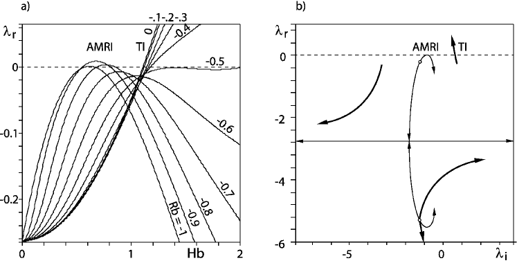
Figure 13: At $\rm Pm=0.05$, $n=1.27842$, $\rm Re=3.8$, and $\rm Ro=-\sqrt{\rm-Rb^{2}-2Rb}$ (a) the growth rates $\lambda_{r}({\rm Hb})$ as $\rm Rb$ changes from $-1$ to $0$; (b) the movement of the roots in the complex plane for (fine lines) ${\rm Rb}=-1$ and (bold lines) ${\rm Rb}=0$.

How the domains of the Tayler instability and AMRI are related to each other? Is there a connection between them in the parameter space?

As is seen in Fig. 10(b), with the decrease in $\rm Rb$, the critical value of $\rm Hb$ at the onset of TI

$${\rm Hb}=\frac{1}{\sqrt{2{\rm Rb}+2\sqrt{{\rm Rb}^{2}+n^{2}}-n^{2}}}.$$ (144)

increases and, as follows from Eqs. (141) and (144), tends to infinity as ${\rm Rb}\rightarrow\frac{n^{2}}{4}-1$. The asymptote

$${\rm Rb}=\frac{n^{2}}{4}-1$$ (145)

is shown in Fig. 10(b) as a horizontal dashed line. If we look at the instability domain in the $\rm Re$-$\rm Hb$ plane at the fixed $\rm Ro$ and $n$, then we will see how the domain of the pure AMRI gradually transforms into that containing the Tayler instability when $\rm Rb$ varies from $-1$ to $0$. The boundary of TI at $\rm Re=0$ originates exactly at the moment when ${\rm Rb}=\frac{n^{2}}{4}-1$, Fig. 10(a).

Let us look at the ${\rm Ro}-{\rm Rb}$ diagram shown in Fig. 3(b). To connect the two opposite corners of it we obviously need to take a path that lies below the line $\rm Ro=Rb$. Indeed, any path above this line penetrates the limiting curve (114) which creates an obstacle for connecting the two regions shown in Fig. 10. On the contrary, any path below the diagonal in Fig. 3(b) lies within the instability domain which opens a possibility to connect the regions of AMRI and standard TI corresponding to $\rm Rb=0$ and $\rm Ro=0$. Therefore, it is the dependency ${\rm Ro}({\rm Rb})$ that controls the transition from the azimuthal magnetorotational instability to the Tayler instability.

Assume, for example, that $\rm Ro=-\sqrt{-\rm Rb^{2}-2\rm Rb}$, which is a part of the unit circle that connects the point with $\rm Rb=-1$ and $\rm Ro=-1$ and the point with $\rm Rb=0$ and $\rm Ro=0$ in Fig. 3(b). Substituting this dependency into the expression (140), we can plot the domain of instability in the $({\rm Hb},{\rm Rb},{\rm Re})$ space for a given $n$, Fig. 11(a). The cross-section of the domain at $\rm Re=0$ yields exactly the region of the Tayler instability shown in Fig. 10(b). The cross-section at $\rm Rb=-1$ is the domain of AMRI in Fig. 10(a).

At $\rm Re<4.99083...$ the azimuthal MRI with $n\approx 1.27842$ at ${\rm Rb}=-1$ does not exist. With the increase in the Reynolds number the island of AMRI originates, Fig. 11(b), that further reconnects with the viscosity-modified domain of TI at a saddle point, Fig. 11(c). At higher values of $\rm Re$ the two domains merge into one, Fig. 11(d).

What happens with the inductionless instability diagram of Fig. 11 when the magnetic Prandtl number takes finite values? It turns out that at $\rm Pm\ll 1$ the difference is very small and is not qualitative. Moreover, at $\rm Re=0$ the domain of the Tayler instability is still given by equation (141) and thus coincides with that shown in Fig. 10(b). Nevertheless, the critical Reynolds number at the saddle point and at the onset of AMRI slightly decreases with the increase in $\rm Pm$, Fig. 12.

Finally, we plot in Fig. 13(a) the growth rates $\lambda_{r}(\rm Hb)$ as $\rm Rb$ varies from $-1$ to $0$. One can see that the growth rates of the Tayler instability monotonously increase and become positive at $\rm Hb>1$. When $\rm Rb$ is smaller than about $-0.5$, the function $\lambda_{r}(\rm Hb)$ has a maximum that can both lie below zero and exceed it in dependence on $\rm Rb$. The latter weak instability is the azimuthal magnetorotational instability.

In Fig. 13(b) the movement of the roots corresponding to TI and AMRI is presented. There are indications that the origin of the both instabilities might be related to the splitting of a multiple zero root. Note that in the inductionless case the detailed analysis of the roots movement and their bifurcation is possible with the use of equations (119) and (123). We leave this for a future work.

11 Conclusion

Using the formal short-wavelength asymptotic expansions of geometric optics, we have derived the local transport PDEs for the amplitude of the localized non-axisymmetric perturbation of a rotating flow under the influence of a constant vertical and an azimuthal magnetic field with arbitrary radial dependence. Looking for the solution of the local transport PDEs in the modal form we have derived a dispersion relation of AMRI that is suitable for testing stability in the case of both ideal and dissipative MHD. The dispersion relation of HMRI in viscous and resistive setup is derived separately by applying the WKB approximation in the radial direction only. Particularly, in the limit of vanishing magnetic Prandtl number as well as for small, but finite $\rm Pm$, we have shown that Keplerian profiles can well be destabilized by HMRI or AMRI if only the azimuthal field profile is slightly flatter than $1/R$. We have also shown that the line where the hydrodynamic and the magnetic Rossby number are equal, plays an essential role for the connectedness of the instability domain. We have found that the marginally stable solution corresponding to $\rm Ro=Rb$ and ${\rm N}_{A}={\rm Rm}$ in the limit when both ${\rm Re}\rightarrow\infty$ and ${\rm Rm}\rightarrow\infty$ is generically destabilized by weak but finite electrical resistivity (and in particular cases already by infinitesimally weak electrical resistivity) resulting in AMRI, which is therefore a dissipation-induced instability. In particular, when ${\rm N}_{A}={\rm Rm}$ and $\rm Ro=Rb=-1$, AMRI is a dissipation-induced instability of the Chandrasekhar equipartition solution of ideal MHD. Finally, we have found an analytical condition on $\rm Rb$ separating the regimes of pure AMRI and Tayler instability.

With view on astrophysical applications one has definitely to note that any flatter than $1/R$ profile of $B_{\phi}$ would require some finite magnetic Reynolds number for the necessary induction effects to occur. Nevertheless, our results still provide a real extension of the applicability of MRI, since the Lundquist numbers are allowed to be arbitrarily small, although the growth rate, which is proportional to the interaction parameter, would then be rather small.

The consequences of our findings for those parts of accretion disks with small magnetic Prandtl numbers are still to be elaborated. The action of MRI in the dead zones of protoplanetary disks is an example for which the extended parameter region might have consequences. Particular attention should also be given to the possibility of quasi-periodic oscillations which might easily result from the sensitive dependence of the action of HMRI on the radial profile of of $B_{\phi}$ and the ratio of the latter to $B_{z}$. We notice however that pure hydrodynamical scenarios of transition to turbulence in the dead zones had also been proposed (Marcus et al., 2013).

As for liquid metal experiments, our results give strong impetus for a special set-up in which the magnetic Rossby number can be adjusted by using two independent electrical currents, one through an central, insulated rod, the second one through the liquid metal. A liquid sodium experiment dedicated exactly to this problem is presently being designed in the framework of the DRESDYN project (Stefani et al., 2012). Apart from this, the recently observed, and numerically confirmed, strong sensitivity of AMRI on a slight symmetry breaking of an external magnetic field (Seilmayer et al., 2014) may also be related to our findings.

Appendix A Connection to the work by Friedlander & Vishik (1995)

Friedlander & Vishik (1995) considered stability with respect to non-axisymmetric perturbation of the general toroidal ideal MHD equilibrium with $\boldsymbol{u}_{0}=R\Omega(R,z)\boldsymbol{e}_{\phi}$ and $\boldsymbol{B}_{0}=B^{0}_{\phi}(R,z)\boldsymbol{e}_{\phi}=R\sqrt{\rho\mu_{0}}A(R,z)\boldsymbol{e}_{\phi}$, where the equilibrium equation requires $\partial_{z}(\Omega^{2}-A^{2})=0$. If we neglect the $z$-dependence and assume that the artificially introduced quantization constant $\tau=0$, their dispersion relation derived in the short-wavelength approximation is given by the characteristic polynomial of the matrix

$${\bf F}=\left(\begin{array}[]{cccc}-im(\Omega-A)&\alpha^{2}(\Omega-A)&0&\alpha^{2}(\Omega+A)\\ A-\Omega&-im(\Omega-A)&-A-\Omega-R\partial_{R}(\Omega+A)&0\\ 0&\alpha^{2}(\Omega-A)&-im(\Omega+A)&\alpha^{2}(\Omega+A)\\ A-\Omega-R\partial_{R}(\Omega-A)&0&-(\Omega+A)&-im(\Omega+A)\\ \end{array}\right),$$

where $\alpha=\frac{k_{z}}{\sqrt{k_{z}^{2}+k_{R}^{2}}}$, $A=\omega_{A_{\phi}}$, and according to Eq. (5) and Eq. (37), $R\partial_{R}\Omega=2\Omega{\rm Ro}$ and $R\partial_{R}A=2\omega_{A_{\phi}}{\rm Rb}$. In the new notation the coefficients of the dispersion relation derived by Friedlander & Vishik (1995) exactly coincide with that given by Eq. (B) were one has to set $\omega_{\nu}=0$, $\omega_{\eta}=0$, and $\omega_{A_{z}}=0$.

To show this, we add/subtract the second of the amplitude equations (3) divided by $\sqrt{\rho\mu_{0}}$ to/from the first one in order to write it via the Elsasser variables $\boldsymbol{a}_{\pm}:=\boldsymbol{u}^{(0)}\pm\frac{\boldsymbol{B}^{(0)}}{\sqrt{\rho\mu_{0}}}$

$$\dot{\boldsymbol{a}}_{+} = -\left(\left[\boldsymbol{u}_{0}-\frac{\boldsymbol{B}_{0}}{\sqrt{\rho\mu_{0}}}\right]\cdot\nabla\right)\boldsymbol{a}_{+}-\left(\mathcal{U}{+}\frac{\mathcal{B}}{\sqrt{\rho\mu_{0}}}\right)\boldsymbol{a}_{-}-\frac{\omega_{\nu}+\omega_{\eta}}{2}\boldsymbol{a}_{+}-\frac{\omega_{\nu}-\omega_{\eta}}{2}\boldsymbol{a}_{-}$$

$$+ \frac{\boldsymbol{k}\boldsymbol{k}^{T}}{|\boldsymbol{k}|^{2}}\left(\left[\mathcal{U}{+}\frac{\mathcal{B}}{\sqrt{\rho\mu_{0}}}\right]\boldsymbol{a}_{-}{+}\left[\mathcal{U}{-}\frac{\mathcal{B}}{\sqrt{\rho\mu_{0}}}\right]\boldsymbol{a}_{+}\right){+}\frac{\boldsymbol{k}\boldsymbol{k}^{T}}{|\boldsymbol{k}|^{2}}\left(\frac{\mathcal{B}}{\sqrt{\rho\mu_{0}}}{-}\left(\frac{\boldsymbol{B}_{0}}{\sqrt{\rho\mu_{0}}}\cdot\nabla\right)\right)\frac{\boldsymbol{a}_{+}{-}\boldsymbol{a}_{-}}{2},$$

$$\dot{\boldsymbol{a}}_{-} = -\left(\left[\boldsymbol{u}_{0}+\frac{\boldsymbol{B}_{0}}{\sqrt{\rho\mu_{0}}}\right]\cdot\nabla\right)\boldsymbol{a}_{-}-\left(\mathcal{U}{-}\frac{\mathcal{B}}{\sqrt{\rho\mu_{0}}}\right)\boldsymbol{a}_{+}-\frac{\omega_{\nu}+\omega_{\eta}}{2}\boldsymbol{a}_{-}-\frac{\omega_{\nu}-\omega_{\eta}}{2}\boldsymbol{a}_{+}$$

$$+ \frac{\boldsymbol{k}\boldsymbol{k}^{T}}{|\boldsymbol{k}|^{2}}\left(\left[\mathcal{U}{+}\frac{\mathcal{B}}{\sqrt{\rho\mu_{0}}}\right]\boldsymbol{a}_{-}{+}\left[\mathcal{U}{-}\frac{\mathcal{B}}{\sqrt{\rho\mu_{0}}}\right]\boldsymbol{a}_{+}\right){+}\frac{\boldsymbol{k}\boldsymbol{k}^{T}}{|\boldsymbol{k}|^{2}}\left(\frac{\mathcal{B}}{\sqrt{\rho\mu_{0}}}{-}\left(\frac{\boldsymbol{B}_{0}}{\sqrt{\rho\mu_{0}}}\cdot\nabla\right)\right)\frac{\boldsymbol{a}_{+}{-}\boldsymbol{a}_{-}}{2}.$$

Looking for the solution $\boldsymbol{a}_{\pm}=\widehat{\boldsymbol{a}}_{\pm}e^{\gamma t+im\phi}$, taking into account that $k_{R}=k_{z}\sqrt{1-\alpha^{2}}\alpha^{-1}$, and eliminating the $z$-components of the vectors $\boldsymbol{a}_{\pm}$ via the constraints $\boldsymbol{a}_{\pm}\cdot\boldsymbol{k}=0$ following from Eq. (3) we arrive at the equation ${\bf F}\widehat{\bf b}=\gamma\widehat{\bf b}$, where $\widehat{\bf b}=(\widehat{a}_{+,R},\widehat{a}_{+,\phi},\widehat{a}_{-,R},\widehat{a}_{-,\phi})^{T}$ and $\bf F$ is the matrix defined above in the case when $\omega_{\nu}=0$ and $\omega_{\eta}=0$.

Appendix B Coefficients of the dispersion relations

The complex characteristic polynomial (81) of the matrix (79) has the following coefficients:

$$a_{0}=1,\quad b_{0}=0,\quad a_{1}=2(\omega_{\eta}+\omega_{\nu}),\quad b_{1}=4m\Omega,$$

$$a_{2}=-4\alpha^{2}\omega_{A_{\phi}}^{2}{\rm Rb}+4\alpha^{2}\Omega^{2}(1+{\rm Ro})+(\omega_{\nu}+\omega_{\eta})^{2}-2(3m^{2}\Omega^{2}-(m\omega_{A_{\phi}}+\omega_{A_{z}})^{2}-\omega_{\nu}\omega_{\eta}),$$

$$b_{2}=\frac{3}{4}a_{1}b_{1},$$

$$a_{3}=2(\omega_{\nu}+\omega_{\eta})(-2\alpha^{2}\omega_{A_{\phi}}^{2}{\rm Rb}-(3m^{2}\Omega^{2}-(m\omega_{A_{\phi}}+\omega_{A_{z}})^{2}-\omega_{\nu}\omega_{\eta}))+8\alpha^{2}\Omega^{2}\omega_{\eta}(1+{\rm Ro}),$$

$$b_{3}=\frac{a_{2}b_{1}}{2}+\frac{b_{1}^{3}}{8}-8\Omega\alpha^{2}(\omega_{A_{z}}+m\omega_{A_{\phi}})\omega_{A_{\phi}},$$

$$a_{4}=((4\Omega^{2}(\omega_{A_{z}}+m\omega_{A_{\phi}})^{2}-4\Omega^{4}m^{2}+4\Omega^{2}\omega_{\eta}^{2}){\rm Ro}+8\omega_{A_{\phi}}\omega_{A_{z}}m\Omega^{2}+4\Omega^{2}\omega_{\eta}^{2}-4\Omega^{4}m^{2})\alpha^{2}$$

$$-\Omega^{2}m^{2}(\omega_{\nu}+\omega_{\eta})^{2}+(m^{2}\Omega^{2}-(\omega_{A_{z}}+m\omega_{A_{\phi}})^{2}-\omega_{\nu}\omega_{\eta})^{2}$$

$$+4({\rm Rb}+1)\omega_{A_{\phi}}^{2}\alpha^{2}(m^{2}\Omega^{2}-(\omega_{A_{z}}+m\omega_{A_{\phi}})^{2})+4\omega_{A_{\phi}}^{2}\alpha^{2}(m^{2}\Omega^{2}-\omega_{\nu}\omega_{\eta}{\rm Rb}),$$

$$b_{4}=-4m\Omega\alpha^{2}[({\rm Ro}+1)(\omega_{\eta}-\omega_{\nu})+({\rm Rb}+1)(\omega_{\eta}+\omega_{\nu})]\omega_{A_{\phi}}^{2}$$

$$-4\omega_{A_{z}}\Omega\alpha^{2}({\rm Ro}(\omega_{\eta}-\omega_{\nu})+2\omega_{\eta})\omega_{A_{\phi}}$$

$$+2m\Omega(4\alpha^{2}\Omega^{2}\omega_{\eta}({\rm Ro}+1)+(\omega_{\nu}+\omega_{\eta})(\omega_{\nu}\omega_{\eta}-m^{2}\Omega^{2}+(\omega_{A_{z}}+m\omega_{A_{\phi}})^{2})).$$ (146)

The coefficients of the complex polynomial (94) are:

$$a_{0}=1,\quad b_{0}=0,\quad a_{1}=2\left(\sqrt{\rm Pm}+\frac{1}{\sqrt{\rm Pm}}\right),\quad b_{1}=4n{\rm Re}\sqrt{\rm Pm},$$

$$a_{2}=2(\beta^{2}{\rm Ha}^{2}-3{\rm Re}^{2}{\rm Pm})n^{2}+4\beta{\rm Ha}^{2}n$$

$$+2(1+(1-2{\rm Rb}\beta^{2}){\rm Ha}^{2})+4{\rm Re}^{2}(1+{\rm Ro}){\rm Pm}+\frac{a_{1}^{2}}{4},\quad b_{2}=6n{\rm Re}(1+{\rm Pm}),$$

$$a_{3}=a_{1}(\beta^{2}{\rm Ha}^{2}-3{\rm Re}^{2}{\rm Pm})n^{2}+2a_{1}\beta{\rm Ha}^{2}n$$

$$+a_{1}(1+(1-2{\rm Rb}\beta^{2}){\rm Ha}^{2})+8{\rm Re}^{2}(1+{\rm Ro})\sqrt{\rm Pm},$$

$$b_{3}=4n^{3}\sqrt{\rm Pm}{\rm Re}(\beta^{2}{\rm Ha}^{2}-{\rm Re}^{2}{\rm Pm})$$

$$+2n{\rm Re}(4{\rm Pm}^{2}{\rm Re}^{2}(1+{\rm Ro})+(1+{\rm Pm})^{2}+2{\rm Pm}(1+{\rm Ha}^{2}))/\sqrt{\rm Pm}$$

$$-8(1-n^{2}+\beta n(1+{\rm Rb}))\beta{\rm Ha}^{2}{\rm Re}\sqrt{\rm Pm},$$

$$a_{4}=((\beta^{2}{\rm Ha}^{2}-{\rm Re}^{2}{\rm Pm})n^{2}+2{\rm Ha}^{2}\beta n+{\rm Ha}^{2}+2{\rm Pm}{\rm Re}^{2})^{2}$$

$$+2(2{\rm Re}^{2}{\rm Pm}{\rm Ro}+1)(({\rm Ha}^{2}\beta^{2}-{\rm Re}^{2}{\rm Pm})n^{2}+2{\rm Ha}^{2}\beta n+{\rm Ha}^{2})-(1+{\rm Pm})^{2}{\rm Re}^{2}n^{2}$$

$$+4{\rm Re}^{2}(1+{\rm Ro})-({\rm Ha}^{2}+2{\rm Pm}{\rm Re}^{2})^{2}+{\rm Ha}^{4}+1-4{\rm Rb}\beta^{2}{\rm Ha}^{2}$$

$$-4{\rm Ha}^{2}\beta^{2}({\rm Ha}^{2}(\beta n+1)^{2}-{\rm Pm}{\rm Re}^{2}n^{2})(1+{\rm Rb}),$$

$$b_{4}=2{\rm Re}(1+{\rm Pm})(\beta^{2}{\rm Ha}^{2}-{\rm Re}^{2}{\rm Pm})n^{3}+4{\rm Re}{\rm Ha}^{2}\beta(1+{\rm Pm})n^{2}$$

$$+2{\rm Re}(2(1+{\rm Ro})(2{\rm Re}^{2}{\rm Pm}-\beta^{2}{\rm Ha}^{2}(1{-}{\rm Pm})){+}(1{+}{\rm Pm})(1+{\rm Ha}^{2}(1-2\beta^{2}(1+{\rm Rb}))))n$$

$$-4\beta{\rm Ha}^{2}{\rm Re}(2+(1-{\rm Pm}){\rm Ro}).$$ (147)

The next equation gives the coefficients of the dispersion relation (97):

$$a_{0}=1,\quad b_{0}=0,\quad a_{1}=2\left(\frac{1}{\rm Re}+\frac{1}{\rm Rm}\right),\quad b_{1}=4n,$$

$$a_{2}=2\left(\frac{\beta^{2}{\rm N}}{\rm Rm}-3\right)n^{2}+\frac{4\beta{\rm N}}{\rm Rm}n$$

$$+\frac{2}{\rm Rm}\left(\frac{1}{\rm Re}+(1-{2{\rm Rb}\beta^{2}}){\rm N}\right)+4(1+{\rm Ro})+\frac{a_{1}^{2}}{4},\quad b_{2}=\frac{3}{4}a_{1}b_{1},$$

$$a_{3}=a_{1}\left(\frac{\beta^{2}{\rm N}}{\rm Rm}-3\right)n^{2}+2a_{1}\beta\frac{{\rm N}}{\rm Rm}n+\frac{a_{1}}{\rm Rm}\left(\frac{1}{\rm Re}+(1-2{\rm Rb}\beta^{2}){\rm N}\right)+\frac{8}{\rm Rm}(1+{\rm Ro}),$$

$$b_{3}=4\left(\frac{\beta^{2}\rm N}{\rm Rm}-1\right)n^{3}+2n\left(4(1+{\rm Ro})+\frac{a_{1}^{2}}{4}+\frac{2}{\rm Rm}\left(\frac{1}{\rm Re}+{\rm N}\right)\right)$$

$$-8(1-n^{2}+\beta n(1+{\rm Rb}))\frac{\beta{\rm N}}{\rm Rm},$$

$$a_{4}=\left(\frac{\beta^{2}\rm N}{\rm Rm}-1\right)^{2}n^{4}+\frac{4\beta\rm N}{\rm Rm}\left(\frac{\beta^{2}\rm N}{\rm Rm}-1\right)n^{3}$$

$$+\left(\frac{2}{\rm Rm}\left(\frac{\beta^{2}\rm N}{\rm Rm}-1\right)\left({\rm N}{+}\frac{1}{\rm Re}{-}2(\beta^{2}(1{+}{\rm Rb}){\rm N}{-}(1{+}{\rm Ro}){\rm Rm})\right){+}\frac{4\rm N^{2}\beta^{2}}{\rm Rm^{2}}-\frac{a_{1}^{2}}{4}\right)n^{2}$$

$$+\frac{4\rm N\beta}{{\rm Rm}^{2}}\left(\rm N+\frac{1}{\rm Re}-2(\beta^{2}(1+{\rm Rb})\rm N-(1+{\rm Ro}){\rm Rm})\right)n$$

$$+\frac{1}{\rm Rm^{2}}\left(\left({\rm N}+\frac{1}{\rm Re}\right)^{2}-4{\rm N}\left(\frac{\beta^{2}\rm Rb}{\rm Re}-\rm RoRm\right)+4(1+\rm Ro)-4{\rm N}^{2}\beta^{2}(1+\rm Rb)\right),$$

$$b_{4}=a_{1}\left(\frac{\beta^{2}{\rm N}}{\rm Rm}-1\right)n^{3}+2a_{1}\frac{\beta{\rm N}}{\rm Rm}n^{2}-\frac{4\beta{\rm N}}{\rm Rm}\left(\frac{2}{\rm Rm}+\left(\frac{1}{\rm Rm}-\frac{1}{\rm Re}\right){\rm Ro}\right)$$

$$+\left(\frac{a_{1}}{\rm Rm}\left(\frac{1}{\rm Re}+(1+2\beta^{2}({\rm Ro}-{\rm Rb})){\rm N}\right)-\frac{8(1+{\rm Ro})}{\rm\rm Rm}\left(\frac{\beta^{2}{\rm N}}{\rm Rm}-1\right)\right)n.$$ (148)

Appendix C Connection to the work by Krueger et al. (1966)

The background flow in the Taylor-Couette cell between two co-axial cylinders of infinite length that rotate about their common axis is

$$\Omega(R)=a+\frac{b}{R^{2}},$$ (149)

where

$$a=\frac{\mu_{\Omega}-\hat{\eta}^{2}}{1-\hat{\eta}^{2}}\Omega_{1},\quad b=\frac{1-\mu_{\Omega}}{1-\hat{\eta}^{2}}R_{1}^{2}\Omega_{1},\quad\hat{\eta}=\frac{R_{1}}{R_{2}},\quad\mu_{\Omega}=\frac{\Omega_{2}}{\Omega_{1}},$$ (150)

and $R_{1}$ and $R_{2}$ and $\Omega_{1}$ and $\Omega_{2}$ are the radii and angular velocities of the inner and outer cylinder, respectively. The centrifugal acceleration of the background flow (149) is compensated by the pressure gradient: $R\Omega^{2}=\frac{1}{\rho}\frac{\partial p_{0}}{\partial R}$. In view of the definition (5)

$$a=\Omega(1+{\rm Ro}).$$ (151)

In case when the gap between the cylinders $d=R_{2}-R_{1}$ is small with respect to the radii, the linearized equations derived by Krueger et al. (1966) for the stability of the viscous Taylor-Couette flow of hydrodynamics with respect to non-axisymmetric disturbances have the form

$$L(D^{2}-(k_{z}d)^{2})u^{\prime}=-(k_{z}d)^{2}T\Omega_{l}(x)v^{\prime},\quad Lv^{\prime}=u^{\prime},$$ (152)

where $D=d/dx$, $R=R_{1}+xd$, $d/dR=d^{-1}d/dx$, $T=-4a\Omega_{1}d^{4}/\nu^{2}$, $u^{\prime}=u2ad\delta/(\nu\Omega_{1})$, $v^{\prime}=v/(R_{1}\Omega_{1})$, $\delta=d/R_{1}$,

$$L=D^{2}-(k_{z}d)^{2}-i(\sigma+k\sqrt{T}~{}\Omega_{l}(x)),\quad\Omega_{l}(x)=1-(1-\mu_{\Omega})x,\quad x\in[0,1],$$ (153)

$\sigma=\omega d^{2}/\nu$, and $k=m\sqrt{-\frac{\Omega_{1}}{4a}}$.

For any $w\sim\exp(ik_{R}R)$, we have

$$Lw = -\frac{d^{2}}{\nu}\left(\nu(k_{R}^{2}+k_{z}^{2})+i(\omega+m\Omega_{1}\Omega_{l})\right)w$$ (154)

$$= -\frac{d^{2}}{\nu}\left(\nu|\boldsymbol{k}|^{2}+i(\omega+m\Omega_{1}\Omega_{l})\right)w=-\frac{d^{2}}{\nu}\left(\omega_{\nu}+i(\omega+m\Omega_{1}\Omega_{l})\right)w.$$

Consequently, if $u,v\sim\exp(ik_{R}R)$, the first equation in (152) becomes

$$-\frac{d^{2}}{\nu}\left(\omega_{\nu}+i(\omega+m\Omega_{1}\Omega_{l})\right)(-d^{2}|\boldsymbol{k}|^{2})\frac{2ad\delta}{\nu\Omega_{1}}u=-k_{z}^{2}d^{2}(-4a\Omega_{1}d^{4})\frac{\Omega_{l}}{\nu^{2}R_{1}\Omega_{1}}v.$$ (155)

Simplifying this equation yields

$$\left(\omega_{\nu}+i(\omega+m\Omega_{1}\Omega_{l})\right)|\boldsymbol{k}|^{2}u=vk_{z}^{2}2\Omega_{1}\Omega_{l}\frac{d}{\delta R_{1}},$$ (156)

and, finally,

$$\left(\omega_{\nu}+i(\omega+m\Omega_{1}\Omega_{l})\right)u=2\alpha^{2}\Omega_{1}\Omega_{l}v,$$ (157)

where $\alpha=k_{z}/|\boldsymbol{k}|$. Analogously, the second equation in (152) takes the form

$$\left(\omega_{\nu}+i(\omega+m\Omega_{1}\Omega_{l})\right)v=-2au\frac{\delta R_{1}}{d},$$ (158)

and, finally,

$$\left(\omega_{\nu}+i(\omega+m\Omega_{1}\Omega_{l})\right)v=-2\Omega(1+{\rm Ro})u.$$ (159)

The equations (157) and (159) constitute the following system

$$\left(\omega_{\nu}+i(\omega+m\Omega_{1}\Omega_{l})\right)u = 2\alpha^{2}\Omega_{1}\Omega_{l}v,$$

$$\left(\omega_{\nu}+i(\omega+m\Omega_{1}\Omega_{l})\right)v = -2\Omega(1+{\rm Ro})u.$$ (160)

Since $\Omega\approx\Omega_{1}\Omega_{l}$, then

$$\left(\omega_{\nu}+i(\omega+m\Omega)\right)u = 2\alpha^{2}\Omega v,$$

$$\left(\omega_{\nu}+i(\omega+m\Omega)\right)v = -2\Omega(1+{\rm Ro})u.$$ (161)

The system (C) can be written in the matrix form ${\bf A}{\bf w}=i\omega{\bf w}$ with the vector ${\bf w}=(u,v)^{T}$ and

$${\bf A}=\left(\begin{array}[]{cc}-im\Omega-\omega_{\nu}&2\alpha^{2}\Omega\\ -2\Omega(1+{\rm Ro})&-im\Omega-\omega_{\nu}\\ \end{array}\right).$$ (162)

The matrix $\bf A$ is nothing else but the submatrix of the matrix $\bf H$ defined by Eq. (79) situated at the corner corresponding to the first two rows and first two columns of $\bf H$.

Let ${\bf A}_{0}={\bf A}(\omega_{\nu}=0)$, then

$${\bf A}_{0}=-{\bf G}^{-1}\overline{\bf A}^{T}_{0}{\bf G},\quad{\bf G}=i{\bf J},\quad{\bf J}=\left(\begin{array}[]{cc}0&-1\\ 1&0\\ \end{array}\right),$$ (163)

meaning that ${\bf F}=-i{\bf G}{\bf A}_{0}=\overline{\bf F}^{T}$ is a Hermitian matrix:

$${\bf F}=\left(\begin{array}[]{cc}2\Omega(1+{\rm Ro})&im\Omega\\ -im\Omega&2\alpha^{2}\Omega\\ \end{array}\right).$$ (164)

Then, the eigenvalue problem ${\bf A}_{0}{\bf w}=i\omega{\bf w}$ acquires the Hamiltonian form

$${\bf Fw}=i\omega{\bf J}{\bf w},\quad{\bf F}=\overline{\bf F}^{T}$$ (165)

and has the eigenvalues $\omega_{1,2}=-m\Omega\pm 2\alpha\Omega\sqrt{1+{\rm Ro}}$, corresponding to Kelvin waves.

References

- (1)
- Acheson (1978) Acheson, D. J. 1978 On the instability of toroidal magnetic fields and differential rotation in stars. Phil. Trans. R. Soc. A 289(1363), 459–500.
- Acheson & Hide (1973) Acheson, D. J. & Hide, R. 1973 Hydromagnetics of rotating fluids. Rep. Prog. Phys. 36, 159–221.
- Altmeyer et al. (2011) Altmeyer, S., Hoffmann, C. & Lücke, M. 2011 Islands of instability for growth of spiral vortices in the Taylor-Couette system with and without axial through flow. Phys. Rev. E 84, 046308.
- Armitage (2011) Armitage, P. J. 2011 Protoplanetary disks and their evolution. Annu. Rev. Astron. Astrophys. 49, 67–117.
- Balbus & Hawley (1991) Balbus, S. A. & Hawley, J. F. 1991 A powerful local shear instability in weakly magnetized disks. 1. Linear Analysis. Astrophys. J., 376, 214–222.
- Balbus & Hawley (1992) Balbus, S. A. & Hawley, J. F. 1992 A powerful local shear instability in weakly magnetized disks. 4. Nonaxisymmetric perturbations. Astrophys. J., 400, 610–621.
- Bayly (1988) Bayly, B. J. 1988 Three-dimensional centrifugal-type instabilities in inviscid two-dimensional flows. Phys. Fluids 31, 56–64.
- Bilharz (1944) Bilharz, H. 1944 Bemerkung zu einem Satze von Hurwitz. ZAMM. 24, 77–82.
- Bogoyavlenskij (2004) Bogoyavlenskij, O. I. 2004 Unsteady equipartition MHD solutions. J. Math. Phys. 45, 381–390.
- Brandenburg et al. (1995) Brandenburg, A., Nordlund, A., Stein, R.F. & Torkelsson, U. 1995 Dynamo-generated turbulence and large-scale magnetic fields in a Keplerian shear flow. Astrophys. J. 446, 741–754.
- Chandrasekhar (1956) Chandrasekhar, S. 1956 On the stability of the simplest solution of the equations of hydromagnetics. Proc. Natl. Acad. Sci. U.S.A. 42, 273–276.
- Chandrasekhar (1960) Chandrasekhar, S. 1960 The stability of non-dissipative Couette flow in hydromagnetics. Proc. Natl. Acad. Sci. U.S.A. 46, 253–257.
- Chandrasekhar (1961) Chandrasekhar, S. 1961 Hydrodynamic and hydromagnetic stability, Oxford University Press, Oxford, UK.
- Dobrokhotov & Shafarevich (1992) Dobrokhotov, S. & Shafarevich, A. 1992 Parametrix and the asymptotics of localized solutions of the Navier-Stokes equations in , linearized on a smooth flow. Math. Notes, 51, 47–54.
- Done, Gierlinski & Kubota (2007) Done, C., Gierlinski, M. & Kubota, A. 2007 Modelling the behaviour of accretion flows in X-ray binaries. Astron. Astrophys. Rev., 15, 1–66.
- Eckhoff (1981) Eckhoff, K. S. 1981 On stability for symmetric hyperbolic systems, I. J. Diff. Eqs. 40, 94–115.
- Eckhoff (1987) Eckhoff, K. S. 1987 Linear waves and stability in ideal magnetohydrodynamics. Phys. Fluids 30, 3673–3685.
- Eckhardt & Yao (1995) Eckhardt, B. & Yao, D. 1995 Local stability analysis along Lagrangian paths. Chaos, Solitons & Fractals, 5(11), 2073–2088.
- Fleming, Stone & Hawley (2000) Fleming, T. P., Stone, J. M., & Hawley, J. F. 2010 The effect of resistivity on the nonlinear stage of the magnetorotational instability in accretion disks. Astrophys. J. 530, 464–477.