Hedging Expected Losses on Derivatives
in Electricity Futures Markets

1 Introduction

We propose in this contribution a method involving numerical implementation for partially hedging financial derivatives on electricity futures contracts. Electricity futures markets present specific features. As a non-storable commodity, electrical energy is delivered as a power over time periods. Similarly, futures contracts exchange a present power price for delivery over a fixed future period against the future quoted price on that period: they refer explicitly to swap contracts, see [2]. Electricity being non-storable, arbitrage arguments do not hold, preventing anyone to construct a term structure via usual tools. As a natural result of liquidity restriction and uncertainty in the future, a limited number of contracts are quoted and the length of their delivery period increases with their time to maturity. This phenomenon we call the granularity of the term structure implies that the most desired and flexible contracts (weekly or monthly-period contracts) are only quoted a short time before their maturity. If one desires a fixed price for power delivered on a given distant month in the future, she shall get a contract covering a wider period, e.g. a quarter or a year contract. However, the risk remains if one is endowed with a derivative upon such a short period contract, before this contract is even quoted.

This is the explored situation: we consider here an agent endowed with a derivative upon a non-yet quoted asset. In practice, the unhedgeable risk of such a position is managed by deploying a cross-hedging strategy with a correlated quoted asset, see [22], [13] and [18]. The risk cannot be completely eliminated without prohibitive cost: the market is incomplete and the methodology requires a pricing criterion, as proposed in the above references. In what follows, we develop a partial hedging procedure in order to satisfy a loss constraint in expectation. We aim at providing a ready-to-implement method to attain such objectives. This necessitates recent tools of stochastic control [5] and numerical approximations of coupled forward backward SDEs. However, we relate constantly the obtained results to well-known formulas and concepts, so that the method is easy to assimilate. We also provide strong and sufficient assumptions in order to avoid involved proofs in difficult cases. We believe that the specific method proposed hereafter can be understood and applied without much effort, and be profitable to a numerous variety of hedging problems.

The approach we adopt has been originated by Föllmer and Leukert [14, 15] but we develop the problem in the framework of control theory. The minimal initial portfolio value needed to satisfy the constraint of expectation of losses can be expressed as a value function of a stochastic target problem. The stochastic target approach has been introduced by Soner and Touzi [20, 21] to formulate the pricing problem in a control fashion. It has been extended to expectation criteria by Bouchard, Elie and Touzi [5], and applied for quantile hedging [5], loss constraints in liquidation problems [3], or loss constraints with small transaction costs [7]. However, the general approach is rather technical and necessitates to solve a non-linear Partial Differential Equations (PDE), when one has first proved a comparison theorem to resolve the uniqueness problem for the value function.

Here, we use the application of [5], where nice results can be provided in complete market without appealing to comparison arguments. However, our initial problem cannot be tackled directly with the stochastic target formulation of [5] or [19]. The unhedgeable risk coming from the apparition of the desired asset price generates a non-trivial extension to the usual framework. Instead, we proceed in three steps in a backward fashion:

1. We first formulate in Section 3 the stochastic target problem in complete market, using an easy extension of the application in [5]. Our approach relies strongly on the convexity of the loss function. By convex duality arguments, the expected loss target can be expressed in order to provide a formula which is very close to a usual risk-neutral pricing formulation. This allows to express the value function $V$ at the precise moment of the apparition of the missing contract.

2. To treat the random apparition of a non-yet traded asset, we use a face-lifting procedure that provides a new (intermediary) target for the period before quotation of the underlying asset. This is done in Section 4, in coherence with the initial hedging criterion, and allows to retrieve a complete market setting where results of step 1 can be partially used.

3. When the complete market setting cannot provide analytical formulas, as it happens after step 2, we shall make use of numerical approximations. We propose such an algorithm in Section 5, and illustrate the efficiency of the method in Section 6.

As it will be understood, this method can be applied recursively by proceeding repeatedly to steps 1 and 2 along the numerical algorithm provided in step 3. The remaining of the contribution follows the above order, preluded by the introduction of the problem in section 2, where we develop the archetypal situation encountered by a financial agent on the market.

2 Description of the control problem

Let $0<T<T^{*}<\infty$. We consider an agent endowed with a financial option with expiration date $T^{\ast}$, payoff $g$ on a futures covering a monthly period. However, this asset is not yet quoted at initial time $t=0$, and appears on the market at time $T$. The month is covered by a futures with delivery over a larger period, e.g. a quarter futures. We denote by $X:=(X_{t})_{t\in[0,T^{\ast}]}$ the discounted price of this instrument, avoiding the introduction of an interest rate hereafter. We assume it is available over the whole period of interest $[0,T^{\ast}]$, whereas the monthly-period futures upon which the agent has a position is only available on the interval $[T,T^{\ast}]$.

The heart of our approach is to assume a structural relation between the two instruments above, namely that the return of the two assets are perfectly correlated. More precisely, the monthly futures price is supposed to be given as the product, $\Lambda X_{t}$, of the quarterly futures price $X_{t}$ and a given shaping factor $\Lambda>0$, assumed to be a bounded random variable revealed at time $T$, completely independent of the asset price $X$. The boundness condition follows from a structural relation between the two futures contracts, assuming implicitly that the underlying spot price is non-negative.

We consider a probability space $(\Omega,{\cal F},{\mathbb{P}})$ supporting a Brownian motion $W$ and the variable $\Lambda$. The filtration ${\mathbb{F}}$ is given by ${\cal F}_{t}:=\sigma(W_{s},\ 0\leq s\leq t)$ for $t<T$, and by ${\cal F}_{t}:=\sigma(W_{s},\ 0\leq s\leq t)\wedge\sigma(\Lambda)$ for $t\geq T$.

Assumption 1.

We denote by $L$ the support of $\Lambda$, which is supposed to be a bounded subset of ${\mathbb{R}}^{+}$, and $\rho$ its probability measure on $L$.

On the period $[0,T]$, the agent trades with the asset $X^{t,x}$, which is assumed to be solution to the SDE:

$$dX^{t,x}_{s}=\mu(s,X^{t,x}_{s})ds+\sigma(s,X^{t,x}_{s})dW_{s},\quad\textrm{for}\ s\geq t,\;\mbox{ and }\;X^{t,x}_{t}=x\;.$$ (1)

We assume the following for $X^{t,x}$ to be well and uniquely defined.

Assumption 2.

The functions $(\mu,\sigma)\ :\ [0,T^{*}]\times{\mathbb{R}}_{+}\rightarrow{\mathbb{R}}\times{\mathbb{R}}_{+}^{*}$ are assumed to be such that the following properties are verified:

1. $\mu$ and $\sigma$ are uniformly Lipschitz and verify $|\mu(t,x)|+|\sigma(t,x)|\leq K(1+|x|)$ for any $(t,x)\in[0,T^{*}]\times{\mathbb{R}}_{+}$.

2. for any $x>0$, we have $X^{t,x}_{s}>0$ $\mathbb{P}-\mbox{a.s.}$ for all $s\in[0,T^{*}]$

3. $\sigma(t,x)>0$ for any $(t,x)\in[0,T^{*}]\times{\mathbb{R}}^{*}_{+}$;

4. if $x=0$ then $\sigma(t,x)=0$ for all $t\in[0,T^{\ast}]$;

5. $\sigma$ is continuous in the time variable on $[0,T^{\ast}]\times{\mathbb{R}}_{+}$;

6. $\mu$ and $\sigma$ are such that

   $$\theta(t,x):=\frac{\mu(t,x)}{\sigma(t,x)}<\infty\quad\text{ uniformly in }(t,x)\in[0,T^{*}]\times{\mathbb{R}}^{*}_{+}\;.$$ (2)

Eq. (2) implies the so-called Novikov condition.The submarket composed of only $(X_{t})_{t\in[0,T^{*}]}$ is then a complete market associated to the Brownian subfiltration. The filtration ${\mathbb{F}}$ relates to an incomplete market because of $\Lambda$, which is unknown on the interval $[0,T)$ and cannot be hedged by a self-financed admissible portfolio defined as follows. In that manner, the market can be labelled as semi-complete in the sense of Becherer [1].

Definition 1.

An admissible self-financed portfolio is a ${\mathbb{F}}$-adapted process $Y^{t,x,y,\nu}$ defined by $Y_{t}^{t,x,y,\nu}=y\geq-\kappa$ and

$$Y^{t,x,y,\nu}_{s}:=y+\int_{t}^{s}\nu_{u}dX^{t,x}_{u}\;,\quad s\in[t,T^{\ast}]\;,$$ (3)

where $\nu\in{\cal U}_{t,y}$ denotes a strategy and ${\cal U}_{t,y}$ the set of admissible strategies at time $t$, which is the set of ${\mathbb{R}}$-valued ${\mathbb{F}}$-progressively measurable, square-integrable processes such that $Y_{s}^{t,x,y,\nu}\geq-\kappa\ \mathbb{P}-\mbox{a.s.}$ for all $s\in[t,T^{\ast}]$ and some $\kappa\geq 0$ representing a finite credit line for the agent.

According to the asset model (1), it is strictly equivalent to consider a hedging portfolio with $X^{t,x}$ on $[0,T^{\ast}]$ or a switch at any time $r\in[T,T^{\ast}]$ for the newly appeared asset $\Lambda X^{t,x}$:

$$Y^{t,x,y,\nu}_{s}=y+\int_{t}^{s\wedge r}\nu_{u}dX^{t,x}_{u}+\int_{s\wedge r}^{t}\nu^{\prime}_{u}d(\Lambda X^{t,x}_{u})\;,r\geq T\;\mbox{ and }\;t\geq 0\;,$$

if $\nu^{\prime}=\nu/\Lambda$ for $u\geq r$. We thus assume that the agent trades with $X$ on $[0,T^{*}]$.

Assumption 3.

The final payoff of the option is given by $g(\Lambda X_{T^{\ast}})$, where the function $g$ is assumed to be Lipschitz continuous.

As it is well-known in the literature, the superhedging price of such an option can be prohibitive, even with Assumption 1 where $\Lambda$ is bounded. To circumvent this problem, we propose to control the expected losses on partial hedging. That means that the agent gives herself a threshold $p<0$ and a loss function $\ell$ to evaluate the loss over her terminal position $g(\Lambda X^{t,x}_{T^{\ast}})-Y^{t,x,y,\nu}_{T^{\ast}}$.

Definition 2.

A loss function $\ell\ :\ {\mathbb{R}}_{+}\rightarrow{\mathbb{R}}_{+}$ is assumed to be continuous, strictly convex and strictly increasing on ${\mathbb{R}}_{+}$ with polynomial growth. We normalize the function so that $\ell(0)=0$.

The agent’s objective at time $t$ is to find the minimal value $y$ and a portfolio strategy $\nu\in{\cal U}_{t,y}$ such that

$$\mathbb{E}\left[-\ell\left(\left(g\left(\Lambda X^{t,x}_{T^{\ast}}\right)-Y^{t,x,y,\nu}_{T^{\ast}}\right)^{+}\right)\right]\geq p\;.$$ (4)

More generally, it will be useful to measure the deviation between the payoff and the hedging portfolio through a general map $\Psi:{\mathbb{R}}_{+}\times{\mathbb{R}}\rightarrow{\mathbb{R}}_{-}$. The previous example corresponds to the specific case where

$$\Psi(x,y)=-\ell((g(x)-y)^{+}).$$ (5)

Assumption 3 and Definition 2 imply that $\Psi$ defined above satisfies the following assumption:

Assumption 4.

The function $\Psi:{\mathbb{R}}_{+}\times{\mathbb{R}}\rightarrow{\mathbb{R}}_{-}$ is assumed to be

• continuous with polynomial growth in $(x,y)$.

• concave and increasing in $y$ on ${\rm cl}\left\{y\in[-\kappa,\infty)\leavevmode\nobreak\ :\leavevmode\nobreak\ \Psi(x,y)<0\right\}$ for any $x\in{\mathbb{R}}_{+}$.

Notice that $\Psi(x,y)=0$ in (5) for any $y\geq g(x)$, which makes $\Psi$ not invertible on the domain ${\mathbb{R}}$ for any fixed $x$. Under Assumption 4, we can define the $y$ inverse $\Psi^{-1}(x,p)$ on ${\mathbb{R}}_{+}\times{\mathbb{R}}_{-}$ as a convex increasing function of $p$, where

$$\Psi^{-1}(x,0)=\inf\left\{y\geq-\kappa\leavevmode\nobreak\ :\leavevmode\nobreak\ \Psi(x,y)=0\right\}\;.$$ (6)

As explained above, the valuation approach of (4) has been introduced in [15, 16]. It can be written under the stochastic control form of [5] allowed by the Markovian framework (1)-(3).

Definition 3.

Let $(t,x,p)\in{\mathbf{S}}:=[0,T^{*}]\times{\mathbb{R}}_{+}^{*}\times{\mathbb{R}}_{-}^{*}$ be given. Then we define the value function $V$ on ${\mathbf{S}}$ as

$$V(t,x,p):=\inf\left\{y\geq-\kappa\leavevmode\nobreak\ :\leavevmode\nobreak\ \mathbb{E}\left[\Psi(\Lambda X^{t,x}_{T^{\ast}},Y^{t,x,y,\nu}_{T^{\ast}})\right]\geq p\text{ for }\nu\in{\cal U}_{t,y}\right\}\;.$$ (7)

Advanced technicalities and details on the general setting for the stochastic target problem with controlled loss can be found in [5] and [19]. In particular, we introduce the value function $V$ only on the open domain of $(x,p)$, and avoid treating the specific case $x=0$ or $p=0$. Furthermore, the function $V$ is implicitely bounded by the superhedging price of $g(\Lambda X^{t,x}_{T^{*}})$ as we will see in the next section. Notice that the expectation in (7) involves an integration w.r.t. the law of $\Lambda$ for $t\in[0,T)$, before the shaping factor $\Lambda$ is revealed. Thus, the present problem is not standard due to the presence of $\Lambda$: the filtration ${\mathbb{F}}$ is not only due to the Brownian motion, and dynamic programming arguments of [5] do not apply directly. The approach we undertake is to separate the complete and incomplete market intervals in a piecewise problem.

Example 1.

A particular example of loss function we will use in sections 5 and 6 is the special case of lower partial moment

$$\ell(x):=x^{k}\mathds{1}_{\left\{x\geq 0\right\}}/k\ ,\quad\textrm{with}\quad k>1\ .$$ (8)

In the case of $k=1$, (which is not considered here) we obtain a criterion close to the expected shortfall, independently studied in [12], whereas allowing $k=0$ allows to retrieve precisely the quantile hedging problem [5], although $\ell$ is not a loss function as in Definition 2 in that case. The case $k=2$ gets closer to the quadratic hedging (or mean-variance hedging) objective, but with the advantage of considering only losses, and not gains. Notice that $\ell$ as in equation (8) for $k>1$ follows Definition 2 and that Assumption 4 holds with (5) if Assumption 3 holds.

We finish this section with additional notations. In the sequel, we will denote ${\mathbf{S}}:={\mathbf{S}}_{1}\cup{\mathbf{S}}_{2}$ where ${\mathbf{S}}_{1}:=[0,T]\times{\mathbb{R}}_{+}^{*}\times{\mathbb{R}}_{-}^{*}$ and ${\mathbf{S}}_{2}:=[T,T^{*}]\times{\mathbb{R}}_{+}^{*}\times{\mathbb{R}}_{-}^{*}$ are the two domains of the value function. For any real valued function $\varphi$, defined on ${\mathbf{S}}$, we denote by $\varphi_{t}$ or $\varphi_{x}$ the partial derivatives with respect to $t$ or $x$. Partial derivatives of other variables, or second order partial derivatives are written in the same manner.

3 Solution in complete market

3.1 General solution and risk-neutral expectation

On the interval $[T,T^{\ast}]$, the variable $\Lambda$ is known and the asset $\Lambda X$ is tradable. We assume that $\Lambda$ takes the value $\lambda\in L$. On this interval, $\lambda$ can be seen as a coefficient affecting the loss function $\Psi$, and the problem (7) follows the standard formulation of [5]: the filtration is generated by the paths of the Brownian motion. In section 4, we reduce the incomplete market setting of period $[0,T)$ to complete market problem of the form (7) on $[T,T^{*}]$, in a similar Brownian framework, with a function $\Psi$ which is no more derived from a loss function as in (5), motivating the introduction of the general function $\Psi$.

Consequently and without loss of generality, we temporarily assume $L=\{1\}$, and omit $\lambda$ in the notation. On $[0,T^{*}]$ then, we can work on problem (7) in the Brownian filtration and apply most results of [5]. The filtration ${\mathbb{F}}$ for $t\geq T$ in that case is given by ${\cal F}_{t}:=\sigma(W_{s}\leavevmode\nobreak\ :\leavevmode\nobreak\ T\leq s\leq t)$ on a complete probability space $(\Omega,{\cal F},{\mathbb{P}})$ with $\mathbb{P}\left[{\Lambda=1}\right]=1$.

Proposition 1.

Under Assumptions 2 and 4, the function $V$ is given on ${\mathbf{S}}$ by

$$V(t,x,p)={\mathbb{E}}^{{\mathbb{Q}}_{t}}\left[\Psi^{-1}\left(X^{t,x}_{T^{*}},J\left(X^{t,x}_{T^{*}},Q^{t,q}_{T^{*}}\right)\right)\right]$$ (9)

where $J(x,q):={\rm arg}\!\sup\limits\left\{pq-\Psi^{-1}(x,p)\leavevmode\nobreak\ :\leavevmode\nobreak\ p\leq 0\right\}$ and

$$X^{t,x}_{s}=x+\int_{t}^{s}\sigma(u,X^{t,x}_{u})dW^{{\mathbb{Q}}_{t}}_{u}\;\mbox{ and }\;Q^{t,q}_{s}=q+\int_{t}^{s}Q^{t,q}_{u}\theta(u,X^{t,x}_{u})dW^{{\mathbb{Q}}_{t}}_{u}\;,$$ (10)

with $W^{{\mathbb{Q}}_{t}}$ being the Brownian motion under the probability ${\mathbb{Q}}_{t}$, the latter being defined by ${d{\mathbb{P}}}_{t}/{d{\mathbb{Q}}_{t}}=Q^{t,1}$ and used for expectation (9). Finally $q$ is given such that ${\mathbb{E}}\left[J\left(X^{t,x}_{T^{*}},Q^{t,q}_{T^{*}}\right)\right]=p$.

To obtain such a result, we proceed in several steps. We first use Proposition 3.1 in [5] to express problem (7) in the standard form of [20], see Lemma 1 below. We then apply the Geometric Dynamic Programming Principle (GDP) Principle of [20] in order to obtain a PDE characterization of $V$ in the viscosity sense. These results are recalled in Appendix. We then use properties of the convex conjugate of $V$ to obtain $V$ as the risk-neutral expectation (9) of Proposition 1.

Lemma 1.

Let $P^{t,p,\alpha}$ be a ${\mathbb{F}}$-adapted stochastic process defined by

$$P^{t,p,\alpha}_{s}=p+\int_{t}^{s}\alpha_{u}P^{t,p,\alpha}_{u}dW_{u}\;,\quad 0\leq t\leq s\leq T^{*}\;,$$ (11)

where $\alpha$ is a ${\mathbb{F}}$-progressively measurable process taking values in ${\mathbb{R}}$. Let us denote ${\cal A}_{t,p}$ the set of such processes such that $P^{t,p,\alpha}$ and $\alpha P^{t,p,\alpha}$ are square-integrable processes. Let Assumptions 2 and 4 hold. Then on ${\mathbf{S}}$

$$V(t,x,p)=\inf\left\{y\geq-\kappa\ :\ Y_{T^{*}}^{t,x,y,\nu}\geq\Psi^{-1}(X^{t,x}_{T^{*}},P_{T^{*}}^{t,p,\alpha})\text{ for }(\nu,\alpha)\in{\cal U}_{t,y}\times{\cal A}_{t,p}\right\}\;.$$ (12)

Moreover, for a given triplet $(t,y,p)$, if there exists $\nu\in{\cal U}_{t,y}$ and a ${\mathbb{F}}$-progressively measurable process $\alpha$ taking values in ${\mathbb{R}}$ such that

$$Y_{T^{*}}^{t,x,y,\nu}\geq\Psi^{-1}(X^{t,x}_{T^{*}},P_{T^{*}}^{t,p,\alpha})\ \mathbb{P}-\mbox{a.s.}\;,$$ (13)

then there exists $\alpha^{\prime}\in{\cal A}_{t,p}$ such that $Y_{T^{*}}^{t,x,y,\nu}\geq\Psi^{-1}(X^{t,x}_{T^{*}},P_{T^{*}}^{t,p,\alpha^{\prime}})$ $\mathbb{P}-\mbox{a.s.}$

Proof.

Under Assumption 4, $\Psi^{-1}(x,p)$ is well defined with (6). According to the polynomial growth of $\Psi$ combined with Assumption 2, the stochastic integral representation theorem can be applied. The first result (12) is then a reformulation of Proposition 3.1 in [5].

The second result echoes Assumption 4 and Remark 6 in [3], as the statement is missing in [5]. According to (11), for $p<0$, the process $P^{t,p,\alpha}$ is a negative local martingale, and therefore a bounded submartingale. Thus, $\mathbb{E}\left[\Psi(X^{t,x}_{T^{*}},Y^{t,x,y,\nu}_{T^{*}})\right]\geq p$. According to the growth condition of $\Psi$, the martingale representation theorem implies the existence of a square-integrable martingale $P^{t,p,\alpha^{\prime}}$, with $P^{t,p,\alpha^{\prime}}_{t}=p$ and according to (13),

$$\mathbb{E}\left[\Psi(X^{t,x}_{T^{*}},Y^{t,x,y,\nu}_{T^{*}})-P_{T^{*}}^{t,p,\alpha^{\prime}}\right]=\mathbb{E}\left[\Psi(X^{t,x}_{T^{*}},Y^{t,x,y,\nu}_{T^{*}})\right]-p\geq 0\;.$$

Since $\Psi(x,y)\in{\mathbb{R}}_{-}$ for any $(x,y)\in{\mathbb{R}}_{+}\times{\mathbb{R}}$, we can choose $P^{t,p,\alpha^{\prime}}$ to follow dynamics (11). This implies that $\alpha^{\prime}$ is a real-valued $({\cal F}_{t})$-progressively measurable process such that $(\alpha^{\prime}P^{t,p,\alpha^{\prime}})\in L^{2}([0,T^{*}]\times\Omega)$, and $\alpha^{\prime}\in{\cal A}_{t,p}$. ∎

We can now turn to the proof of Proposition 1 by using the GDP recalled in Appendix. The proof follows closely developments of section 4 in [5], and is given for the sake of clarity, as for the introduction of important objects for section 4.3.

Proof.

(Proposition 1) We divide the proof in three steps

1. We introduce conjugate and local test functions. Let $V_{*}$ be the lower semi-continuous version of $V$, as defined in Appendix. According to Assumption 4, dynamics (3) and definition (7), $V$ and $V_{*}$ are increasing functions of $p$ on ${\mathbb{R}}_{-}$. The boundedness of $V$ implies also the finitness of $V_{*}$. For $(t,x,q)\in[0,T^{*}]\times{\mathbb{R}}_{+}^{*}\times{\mathbb{R}}_{+}^{*}$, we introduce the convex conjugate of $V_{*}$ in $p<0$, i.e.,

$$\tilde{V}(t,x,q):=\sup\left\{pq-V_{*}(t,x,p)\leavevmode\nobreak\ :\leavevmode\nobreak\ p\leq 0\right\}\;.$$

The map $q\mapsto\tilde{V}(.,q)$ is convex and upper-semi-continuous on ${\mathbb{R}}_{+}^{*}$.

Let $\tilde{\varphi}$ be a smooth function with bounded derivatives, such that $(t_{0},x_{0},q_{0})\in[0,T^{*})\times{\mathbb{R}}_{+}^{*}\times{\mathbb{R}}_{+}^{*}$ is a local maximizer of $\tilde{V}-\tilde{\varphi}$ with $(\tilde{V}-\tilde{\varphi})(t_{0},x_{0},q_{0})=0$. The map $q\mapsto\tilde{\varphi}(.,q)$ is convex. Without loss of generality, we can assume that $\tilde{\varphi}$ is strictly convex with quadratic growth in $q$, see the proof in Section 4 of [5].

The convex conjugate of $\tilde{\varphi}$ with respect to $q$ is a strictly convex function of $p$ defined by $\varphi(t,x,p):=\sup\left\{qp-\tilde{\varphi}(t,x,q)\leavevmode\nobreak\ :\leavevmode\nobreak\ q\geq 0\right\}$. We can then properly define the map $(t,x,q)\mapsto(\varphi_{p})^{-1}(t,x,q)$ on $[0,T^{*}]\times{\mathbb{R}}_{+}^{*}\times{\mathbb{R}}_{+}^{*}$, where the inverse is taken in the $p$ variable. According to the definition of $\tilde{V}$ and the quadratic growth of $\tilde{\varphi}$, there exists $p_{0}\leq 0$ such that for the fixed $q_{0}$,

$$p_{0}q_{0}-V_{*}(t_{0},x_{0},p_{0})=\tilde{V}(t_{0},x_{0},q_{0})=\tilde{\varphi}(t_{0},x_{0},q_{0})=\sup_{p\leq 0}\left\{pq_{0}-\varphi(t_{0},x_{0},p)\right\}$$

which, by taking the left and right sides of the above equation, implies that $(t_{0},x_{0},p_{0})$ is a local minimizer of $V_{*}-\varphi$ and $(V_{*}-\varphi)(t_{0},x_{0},p_{0})=0$. The first order condition in the definition of $\varphi$ implies that $p_{0}=(\varphi_{p})^{-1}(t_{0},x_{0},q_{0})$.

2. We prove that $\tilde{V}$ is subsolution to a linear PDE. In our case, the control $\nu$ takes unbounded values by definition of ${\cal U}_{t,y}$. It implies, together with Assumption 2, that

$${\cal N}_{0}(t,x,p,d_{x},d_{p}):=\left\{(u,a)\in{\mathbb{R}}^{2}\leavevmode\nobreak\ :\leavevmode\nobreak\ \left|\sigma(t,x)\left(u-d_{x}\right)-apd_{p}\right|=0\right\}\neq\emptyset$$ (14)

for any $(t,x,p,d_{x},d_{p})\in[0,T^{*}]\times{\mathbb{R}}_{+}\times{\mathbb{R}}_{-}\times{\mathbb{R}}^{2}$. This holds in particular for the set

$${\cal N}_{0}(t_{0},x_{0},p_{0},\varphi_{x}(t_{0},x_{0},p_{0}),\varphi_{p}(t_{0},x_{0},p_{0}))$$

which is then composed of elements of the form $((\varphi_{x}+ap\varphi_{p}/\sigma)(t_{0},x_{0},p_{0}),a)$ for $a\in{\mathbb{R}}$. According to Theorem 2 in Appendix and changing $\nu$ for its new expression, $\varphi$ in $(t_{0},x_{0},p_{0})$ verifies

$$-\varphi_{t}-\frac{1}{2}\sigma^{2}(t_{0},x_{0})\varphi_{xx}-\inf_{a\in{\mathbb{R}}}\left\{\frac{1}{2}(ap_{0})^{2}\varphi_{pp}-ap_{0}(\theta(t_{0},x_{0})\varphi_{p}-\sigma\varphi_{xp})\right\}\geq 0\ .$$ (15)

Since $\varphi_{pp}(t_{0},x_{0},p_{0})>0$, the infimum in the above equation is reached for

$$a:=-\left(\frac{\sigma\varphi_{xp}-\theta\varphi_{p}}{p_{0}\varphi_{pp}}\right)(t_{0},x_{0},p_{0})\in{\mathbb{R}}\;,$$ (16)

which can be plugged back into (15) to obtain a new inequality at $(t_{0},x_{0},p_{0})$:

$$-\varphi_{t}-\frac{1}{2}\sigma^{2}(t_{0},x_{0})\varphi_{xx}+\frac{1}{2}(\varphi_{pp})^{-1}\big{(}\theta(t_{0},x_{0})\varphi_{p}-\sigma(t_{0},x_{0})\varphi_{xp}\big{)}^{2}\geq 0\;.$$ (17)

Recall that $p_{0}=(\varphi_{p})^{-1}(t_{0},x_{0},q_{0})$. According to the Fenchel-Moreau theorem, $\tilde{\varphi}$ is its own biconjugate, $\tilde{\varphi}(t,x,q)=\sup\left\{pq-\varphi(t,x,p)\leavevmode\nobreak\ :\leavevmode\nobreak\ p\leq 0\right\}$, and $\tilde{\varphi}(t_{0},x_{0},q_{0})=p_{0}q_{0}-\varphi(t_{0},x_{0},p_{0})$. By differentiating in $p$, we get $\varphi_{p}(t_{0},x_{0},p_{0})=q_{0}$. It follows by differentiating again that at point $(t_{0},x_{0},p_{0})$ we have the following correspondence:

$$\left(\varphi_{t},\varphi_{x},\varphi_{xx},\varphi_{pp},\varphi_{xp}\right)=\left(-\tilde{\varphi}_{t},-\tilde{\varphi}_{x},-\tilde{\varphi}_{xx}+\frac{\tilde{\varphi}_{xq}^{2}}{\tilde{\varphi}_{qq}},\frac{1}{\tilde{\varphi}_{qq}},-\frac{\tilde{\varphi}_{xq}}{\tilde{\varphi}_{qq}}\right)\;.$$ (18)

Plugging (18) into (17), we get that $\tilde{\varphi}$ satisfies at $(t_{0},x_{0},q_{0})$

$$-\tilde{\varphi}_{t}-\frac{1}{2}\left(\sigma^{2}\tilde{\varphi}_{xx}+|\theta|^{2}q_{0}^{2}\tilde{\varphi}_{qq}+2\mu\tilde{\varphi}_{xq}\right)(t_{0},x_{0},q_{0})\leq 0\;.$$ (19)

By arbitrariness of $(t_{0},x_{0},q_{0})\in[0,T^{*})\times{\mathbb{R}}_{+}^{*}\times{\mathbb{R}}_{+}^{*}$, this implies that $\tilde{V}$ is a subsolution of (19) on $[0,T^{*})\times{\mathbb{R}}_{+}^{*}\times{\mathbb{R}}_{+}^{*}$. The terminal condition is given by the definition of $\tilde{V}$ and Theorem 2 in Appendix:

$$\tilde{V}(T^{*},x,q)=\sup_{p\leq 0}\left\{pq-V_{*}(T^{*},x,p)\right\}=\sup_{p\leq 0}\left\{pq-\Psi^{-1}(x,p)\right\}\;.$$ (20)

3. We compare $V$ to a conditional expectation. Let $\bar{V}$ be the function defined by $\bar{V}(t,x,q)={\mathbb{E}}^{{\mathbb{Q}}_{t}}\left[\tilde{V}(T^{*},X^{t,x}_{T^{*}},Q^{t,q}_{T^{*}})\right]$ for $(t,x,q)\in[0,T^{*}]\times(0,\infty)^{2}$, with dynamics for $s\in[0,T^{*}]$ given by

$$X^{t,x}_{s}=x+\int_{t}^{s}\sigma(u,X^{t,x}_{u})dW^{{\mathbb{Q}}_{t}}_{u}\;\mbox{ and }\;Q^{t,q}_{s}=q+\int_{t}^{s}Q^{t,q}_{u}\theta(u,X^{t,x}_{u})dW^{{\mathbb{Q}}_{t}}_{u}\;,$$

where ${\mathbb{Q}}_{t}$ is a ${\mathbb{P}}$-equivalent measure such that ${d{\mathbb{P}}}/{d{\mathbb{Q}}_{t}}=Q^{t,1}$. According to the Feynman-Kac formula, $\bar{V}$ is a supersolution to equation (19), and thus $\bar{V}\geq\tilde{V}$. According to Assumption 4, $p\mapsto\Psi^{-1}(.,p)$ is convex increasing on ${\mathbb{R}}_{-}$. Thus, for sufficiently large values of $q$, $J(x,q):=\arg\sup\left\{pq-\Psi^{-1}(x,p)\leavevmode\nobreak\ :\leavevmode\nobreak\ p\leq 0\right\}$ is well-defined and can take any value in ${\mathbb{R}}_{-}$. By the implicit function theorem, there exists a function $q$ of $(t,x,p)$ such that ${\mathbb{E}}^{{\mathbb{Q}}_{t}}\left[Q^{t,1}_{T^{*}}J\left(X^{t,x}_{T^{*}},Q^{t,q(t,x,p)}_{T^{*}}\right)\right]=p$. Therefore,

$$\begin{array}[]{lcl}V(t,x,p)&\geq&V_{*}(t,x,p)\geq\sup\left\{qp-\bar{V}(t,x,q)\leavevmode\nobreak\ :\leavevmode\nobreak\ q\geq 0\right\}\\ &\geq&pq(t,x,p)-{\mathbb{E}}^{{\mathbb{Q}}_{t}}\left[\tilde{V}\left(T^{*},X^{t,x}_{T^{*}},Q^{t,q(t,x,p)}_{T^{*}}\right)\right]\\ &\geq&q(t,x,p)\left(p-{\mathbb{E}}^{{\mathbb{Q}}_{t}}\left[Q^{t,1}_{T^{*}}J\left(X^{t,x}_{T^{*}},Q^{t,q(t,x,p)}_{T^{*}}\right)\right]\right)\\ &&\hskip 28.45274pt+{\mathbb{E}}^{{\mathbb{Q}}_{x}}\left[\Psi^{-1}\left(X^{t,x}_{T^{*}},J\left(X^{t,x}_{T^{*}},Q^{t,q(t,x,p)}_{T^{*}}\right)\right)\right]\\ &\geq&{\mathbb{E}}^{{\mathbb{Q}}_{t}}\left[\Psi^{-1}\left(X^{t,x}_{T^{*}},J\left(X^{t,x}_{T^{*}},Q^{t,q(t,x,p)}_{T^{*}}\right)\right)\right]=:y(t,x,p)\;.\end{array}$$

By the martingale representation theorem, there exists $\nu\in{\cal U}_{t,y}$ such that

$$Y^{t,y(t,x,p),\nu}_{T^{*}}=\Psi^{-1}\left(X^{t,x}_{T^{*}},J\left(X^{t,x}_{T^{*}},Q^{t,q(t,x,p)}_{T^{*}}\right)\right)$$

which implies that for $p\leq 0$

$$\begin{array}[]{ll}\mathbb{E}\left[\Psi\left(X^{t,x}_{T^{*}},Y^{t,y(t,x,p),\nu}_{T^{*}}\right)\right]&\geq\mathbb{E}\left[J\left(X^{t,x}_{T^{*}},Q^{t,q(t,x,p)}_{T^{*}}\right)\right]={\mathbb{E}}^{{\mathbb{Q}}_{t}}\left[Q^{t,1}_{T^{*}}J\left(X^{t,x}_{T^{*}},Q^{t,q(t,x,p)}_{T^{*}}\right)\right]\\ &\geq p\end{array}$$

and therefore, by definition of the value function $y(t,x,p)\geq V(t,x,p)$ which provides the equality and (9) for $(t,x,p)\in{\mathbf{S}}$. ∎

3.2 Application to the interval $[T,T^{*}]$

We now come back to $[T,T^{*}]$, where the shaping factor $\Lambda$, is assumed to take the known value $\lambda$ at time $T$. To highlight the effect of $\lambda$ as a given state parameter for $t\geq T$, we denote by $V(t,x,p,\lambda)$ the value function defined similarly as (7) where $\Psi$ is given by (5).

Definition 4.

Let $(t,x,p,\lambda)\in{\mathbf{S}}_{2}\times L$. We can define the value function on ${\mathbf{S}}_{2}\times L$ as

$$V(t,x,p,\lambda):=\inf\{y\geq-\kappa\leavevmode\nobreak\ :\leavevmode\nobreak\ \mathbb{E}\left[\ell\left(g\left(\lambda X^{t,x}_{T^{\ast}}\right)-Y^{t,x,y,\nu}_{T^{\ast}}\right)^{+}\right]\leq-p\ \text{ for }\nu\in{\cal U}_{t,y}\}\;,$$ (21)

Notice that if $X$ is an exponential process, then we can explicitely change $V(t,x,p,\lambda)$ for $V(t,\lambda x,p,1)$, recalling the assumption $\mathbb{P}\left[{\Lambda=1}\right]=1$ of the previous section. Let us recall the standard pricing concepts in complete market. Under Assumption 2, we can define ${\mathbb{Q}}$ the ${\mathbb{P}}$-equivalent martingale measure defined by

$$\left.\frac{d{\mathbb{Q}}}{d{\mathbb{P}}}\right|_{{\cal F}_{t}}=\exp\left\{-\int_{T}^{t}\theta(s,X_{s})dW_{s}-\frac{1}{2}\int_{T}^{t}|\theta(s,X_{s})|^{2}ds\right\}\;,t\geq T\;.$$ (22)

In the present setting, ${\mathbb{Q}}$ is the unique risk-neutral measure with the drifted Brownian motion $W_{t}^{{\mathbb{Q}}}=W_{t}+\int_{T}^{t}\theta(s,X_{s})ds$, and we can provide a unique no-arbitrage price for $g(\lambda X_{T^{\ast}})$.

Definition 5.

We define for $(t,x,\lambda)\in[T,T^{*}]\times{\mathbb{R}}_{+}^{*}\times L$ the function

$$C(t,x,\lambda):={\mathbb{E}}^{{\mathbb{Q}}}[g(\lambda X^{t,x}_{T^{\ast}})]\quad\text{ for }\ t\geq T\;.$$ (23)

According to Assumption 2 and Assumption 3, we can apply Proposition 6.2, in [17], which implies that for any $\lambda\in L$, $(t,x)\mapsto C(t,x,\lambda)$ is Lipschitz continuous in the spatial variable with the same Lipschitz constant $K$ as $g$. Moreover, $C(\cdot,\cdot,\lambda)$ is the unique classical solution of polynomial growth to the Black-Scholes equation

$$-C_{t}-\frac{1}{2}\sigma^{2}(t,x)C_{xx}=0\ \text{ on }\ [T,T^{*})\times(0,+\infty)$$ (24)

with terminal condition $C(T^{*},x,\lambda)=g(\lambda x)$. Now Proposition 1 applies to provide the following when we use a loss function as in Definition 2.

Corollary 1.

Let Assumptions 2 and 3 hold. Then $V$ is given on ${\mathbf{S}}_{2}\times L$ by

$$V(t,x,p,\lambda)={\mathbb{E}}^{{\mathbb{Q}}}[g(\lambda X^{t,x}_{T^{*}})-\ell^{-1}(-P_{T^{*}}^{t,p})]$$ (25)

where $P^{t,p}_{T^{*}}$ is a ${\cal F}_{T^{\ast}}$-measurable random variable defined by

$$P^{t,p}_{T^{*}}=j\left(q\exp\left(\int_{t}^{T^{\ast}}\theta(s,X^{t,x}_{s})dW^{{\mathbb{Q}}}_{s}-\frac{1}{2}\int_{t}^{T^{\ast}}\theta^{2}(s,X^{t,x}_{s})ds\right)\right)$$ (26)

with $j(q):=-((\ell^{-1})^{\prime})^{-1}(q)$ and $q$ in (26) such that ${\mathbb{E}}^{{\mathbb{Q}}}\left[P^{t,p}_{T^{*}}\right]=p\;.$ Moreover, $V$ is convex and increasing in $p$ and is ${\cal C}^{1,2}$ in $(t,x)$ on $[T,T^{*}]\times{\mathbb{R}}_{+}^{*}$.

The solution (25)-(26) can be explicitly computed in simple cases, see section 5 below. Notice that $V$ is bounded on $[T,T^{\ast}]\times{\mathbb{R}}_{+}^{*}\times{\mathbb{R}}_{-}^{*}\times L$ by $C$. Since $\ell$ is convex increasing on ${\mathbb{R}}_{+}$, $-\ell^{-1}$ is convex. A look at (25)-(26) then convinces that $V$ is continuous in $p$ on ${\mathbb{R}}_{-}^{*}$, but Proposition 3.3 in [5] can be used in our setting to assert that $V$ is also convex in $p$. According to what was said about the function $C$, $V$ is ${\cal C}^{1,2}$ in $(t,x)$ on $[T,T^{*}]\times{\mathbb{R}}_{+}^{*}$.

Remark 1.

It is noticeable that the value function (25) is composed of the Black-Scholes price of the claim $g(\lambda X^{t,x}_{T^{*}})$ minus a term that corresponds to a penalty in the dual expression of the acceptance set if $\ell$ is a risk measure, see [16]. The hedging strategy is to be modified in consequence. First note that (25) is a conditional expectation of a function of two Markov processes $(X^{t,x},Q^{t,q})$, for $q$ well chosen, so that we can write $Y^{t,V(t,x,p),\nu}_{s}:=y(X^{t,x}_{s},Q^{t,q}_{s}):=V(s,X^{t,x}_{s},P^{t,p}_{s})$. According to Corollary 1, $y$ is a regular function, and $X^{t,x},Q^{t,q}$ are martingales under the probability ${\mathbb{Q}}$, as well as $Y^{t,V(t,x,p),\nu}$. Therefore Itô formula provides

$$dY^{t,V(t,x,p),\nu}_{s}=y_{x}(X^{t,x}_{s},Q^{t,q}_{s})dX^{t,x}_{s}+y_{q}(X^{t,x}_{s},Q^{t,q}_{s})dQ^{t,q}_{s}\;.$$

Now expressing $dW^{{\mathbb{Q}}}_{s}$ with respect to $dX^{t,x}_{s}$, we obtain

$$dY^{t,V(t,x,p),\nu}_{s}=\left(y_{x}(X^{t,x}_{s},Q^{t,q}_{s})+\mu(s,X^{t,x}_{s})Q^{t,q}_{s}y_{q}(X^{t,x}_{s},Q^{t,q}_{s})\right)dX^{t,x}_{s}$$ (27)

which allows to deduce the optimal dynamic strategy $\nu$.

Corollary 1 retrieves solutions of [15]. The original problem in the latter is to minimize the expected loss given an initial portfolio value, but the authors prove that our version of the problem is equivalent. The stochastic target problem of Definition 3 is actually linked to an optimal control problem in a similar way, as noticed in the introduction of [5] and developped in [4]. We can introduce the value function giving the minimal loss that can be achieved at time $T^{\ast}$, with at time $t$, the initial capital $y$, $X^{t,x}_{t}=x$ and the shaping factor $\Lambda=\lambda$.

Definition 6.

For $(t,x,y,\lambda)\in[T,T^{*}]\times{\mathbb{R}}_{+}^{*}\times{\mathbb{R}}\times L$ we define

$$U(t,x,y,\lambda):=\sup\left\{\mathbb{E}\left[-\ell\left(\left(g\left(\lambda X^{t,x}_{T^{*}}\right)-Y_{T^{\ast}}^{t,y,\nu}\right)^{+}\right)\right]\leavevmode\nobreak\ :\leavevmode\nobreak\ \nu\in{\cal U}_{t,y}\right\}\ .$$ (28)

This corresponds to the problem of finding the best reachable threshold $p$ if the initial portfolio value is given by $y$ at time $t$. This result is of great use in the forthcoming resolution of the problem before $T$, by the following connection with $V$.

Lemma 2.

For $(t,x,y,\lambda)\in[T,T^{*}]\times{\mathbb{R}}_{+}^{*}\times[-\kappa,\infty)\times L$ we define

$$V^{-1}(t,x,y,\lambda):=\sup\left\{p\leq 0\leavevmode\nobreak\ :\leavevmode\nobreak\ V(t,x,p,\lambda)\leq y\right\}\;.$$

Then we have

$$U(t,x,y,\lambda)=V^{-1}(t,x,y,\lambda)\;.$$ (29)

Moreover the function $U$ is a concave increasing function of $y$ bounded by $0$ from above.

Equality (29) is a direct application of Lemma 2.1 in [4], whereas the properties of $U$ fall from the properties of $V$ and Definition 6.

4 Solution in incomplete market

We now turn to the solution of the problem before $T$, i.e., when $\Lambda$ is unkown. We first provide the face-lifting procedure that allows to reduce the new situation to the one handled in Section 3. This procedure can be done according to two model paradigms:

1. the law $\rho$ of $\Lambda$ is supposed to be known;

2. only the support $L$ of the law of $\Lambda$ is supposed to be known.

The first approach is a probabilistic approach with a prior distribution, whereas the second one is a robust approach, in connection with robust finance with parameter uncertainty, see [6] for a control theory version. Finally, the numerical complexity of the face-lifting procedure pushes us to give up explicit formulas for a numerical approach. We thus modify results of Section 3 to provide a convenient formulation of the problem to be numerically approximated in Section 5.

4.1 Faced-lifted intermediary condition with prior on the shaping factor

When $t<T$, the problem (7) cannot be treated with the methodology developped in [5]. To solve the problem, we are guided by the following argument. Considering $(t,y)\in[0,T)\times[-\kappa,\infty)$ and a strategy $\nu\in{\cal U}_{t,y}$, we arrive at time $T$ to the wealth $Y^{t,x,y,\nu}_{T}\geq-\kappa$, at the apparition of the exogenous risk factor $\Lambda$. Assume that the agent wants to control the expected level of risk $p<0$, at time $T$, by using the portfolio $Y^{t,x,y,\nu}_{T}$. It is obviously not possible with certainty if $\Lambda$ takes a value $\lambda$ such that $Y_{T}^{t,y,\nu}<V(T,X^{t,x}_{T},p,\lambda)\;.$ However, the optimal strategy after $T$ consists in optimizing the portfolio by trying to achieve the optimal expected level of loss $U(T,X^{t,x}_{T},Y_{T}^{t,y,\nu},\lambda)$ given by Definition 6. In the complete market setting, this achievement is possible.

Lemma 3.

Under Assumptions 2 and 4, there exists a map $(x,y,\lambda)\mapsto\nu(x,y,\lambda)\in{\cal U}_{T,y}$ on ${\mathbb{R}}_{+}^{*}\times[-\kappa,\infty)\times L$ such that

$$\mathbb{E}\left[\Psi\left(\lambda X^{T,x}_{T^{*}},Y^{T,y,\nu(x,y,\lambda)}_{T^{*}}\right)\right]\geq U(T,x,y,\lambda)\;.$$ (30)

Proof.

Fix $(x,y,\lambda)\in{\mathbb{R}}_{+}^{*}\times[-\kappa,\infty)\times L$. Let $p:=U(T,x,y,\lambda)$. According to Lemma 2, $y\geq V(T,x,p,\lambda)$. Following Corollary 1 and Remark 1, and since $\Psi$ is increasing in $y$, there exists $\nu$ such that $\mathbb{E}\left[\Psi\left(\lambda X^{T,x}_{T^{*}},Y^{T,y,\nu}_{T^{*}}\right)\right]\geq p$ for $(x,y,\lambda)$ arbitarily fixed. ∎

Then the expected loss at $T$ resulting from this strategy is averaged among the the realizations of $\Lambda$ for fixed $X^{t,x}_{T}$ and $Y_{T}^{t,y,\nu}$. The expectation is thus done also with regard to $\Lambda$ just before $T$.

Definition 7.

We define $\Xi:{\mathbb{R}}_{+}\times[-\kappa,\infty)\rightarrow{\mathbb{R}}_{-}$ by

$$\Xi(x,y):=\int_{L}U(T,x,y,r)\rho(dr)\;.$$ (31)

The above function $\Xi$ represents the expected optimal level of loss the agent can reach if she attains the wealth $y$ at time $T$ with a state $X^{T,x}_{T}=x$.

Lemma 4.

The function $\Xi$ takes non-positive values, is ${\cal C}^{2}$ in $x\in{\mathbb{R}}_{+}^{*}$ and concave increasing in $y$.

This is a direct consequence of Lemma 2 and corollary 1. This property ensures that parts of Assumption 4 hold in the new following problem, in order to apply Theorem 2 of Appendix. In particular, Lemma 4 allows to define a terminal condition with the generalized inverse $\Xi^{-1}$.

Definition 8.

For $(t,x,p)\in{\mathbf{S}}_{1}$, we define

$$\bar{V}(t,x,p):=\inf\left\{y\geq-\kappa\leavevmode\nobreak\ :\leavevmode\nobreak\ \mathbb{E}\left[\Xi(X^{t,x}_{T},Y^{t,x,y,\nu}_{T})\right]\geq p\text{ for }\nu\in{\cal U}_{t,y}\right\}\;.$$ (32)

We now prove that this new problem coincides with the one of Definition 3 on $S_{1}$.

Proposition 2.

Let Assumptions 2 and 4 hold. Then $\bar{V}(t,x,p)=V(t,x,p)$ on ${\mathbf{S}}_{1}$.

Proof.

1. Fix $(t,x,p)\in{\mathbf{S}}_{1}$ and take $y>V(t,x,p)$. Then by definition there exists $\nu\in{\cal U}_{t,y}$ such that $\mathbb{E}\left[\Psi\left(X^{t,x}_{T^{*}},Y^{t,x,y,\nu}_{T^{*}}\right)\right]\geq p$. Since $t<T$, the control can be written $\nu_{t}=\nu_{t}\mathds{1}_{\left\{t\in[0,T)\right\}}+\nu_{t}(\Lambda)\mathds{1}_{\left\{t\in[T,T^{*}]\right\}}$ where $\nu_{t}(.)$ follows from the canonical construction of ${\mathbb{F}}$: it is a measurable map from $L$ to the set of square integrable control processes on $[T,T^{*}]$ which are adapted to the Brownian filtration $\sigma(W_{s},\ T\leq s\leq.)$. From the flow property of Markov processes $X^{t,x}$ and $Y^{t,x,y,\nu}$ (see [20]) and the tower property of expectation,

$$\begin{array}[]{ll}\mathbb{E}\left[\Psi\left(X^{t,x}_{T^{*}},Y^{t,x,y,\nu}_{T^{*}}\right)\right]=\\ \displaystyle\mathbb{E}\left[\int_{L}{\mathbb{E}}\left[\Psi\left(X^{T,X^{t,x}_{T}}_{T^{*}},Y^{T,X^{t,x}_{T},Y^{t,x,y,\nu}_{T},\nu(\lambda)}_{T^{*}}\right)\Big{|}\left(X^{t,x}_{T},Y^{t,x,y,\nu}_{T},\lambda\right)\right]\rho(d\lambda)\right]\;.\end{array}$$ (33)

By taking the supremum over all possible maps $\nu(\lambda)$ and by Definition 6, we obtain

$$p\leq{\mathbb{E}}\left[\Psi\left(X^{T,X^{t,x}_{T}}_{T^{*}},Y^{T,Y^{t,x,y,\nu}_{T},\nu(\lambda)}_{T^{*}}\right)\Big{|}\left(X^{t,x}_{T},Y^{t,x,y,\nu}_{T},\lambda\right)\right]\leq U\left(T,X^{t,x}_{T},Y^{t,x,y,\nu}_{T},\lambda\right)\;.$$ (34)

By integrating in $\lambda$ over $L$, and then take the expectation, we immediately get that $y\geq\bar{V}(t,x,p)$. By arbitrariness of $y$, $V(t,x,p)\geq\bar{V}(t,x,p)$.

2. Take $y>\bar{V}(t,x,p)$. There exists a control $\nu\in{\cal U}_{t,y}$ on $[t,T]$ such that

$$\mathbb{E}\left[\int_{L}U\left(T,X^{t,x}_{T},Y^{t,x,y,\nu}_{T},\lambda\right)\rho(d\lambda)\right]\geq p\;.$$

Now Lemma 3 allows to assert the existence of a control $\nu^{*}(\lambda)$ on $[T,T^{*}]$ such that for any $\lambda\in L$

$$\mathbb{E}\left[\Psi\left(X^{T,X^{t,x}_{T}}_{T^{*}},Y^{T,Y^{t,x,y,\nu}_{T},\nu^{*}(\lambda)}_{T^{*}}\right)\right]=U\left(T,X^{t,x}_{T},Y^{t,x,y,\nu}_{T},\lambda\right)\;.$$

By chosing the new admissible control $\nu^{\prime}\in{\cal U}_{t,y}$ defined by the concatenation $\nu^{\prime}_{t}=\nu_{t}\mathds{1}_{\left\{t\in[0,T)\right\}}+\nu^{*}_{t}(\Lambda)\mathds{1}_{\left\{t\in[T,T^{*}]\right\}}$, we obtain $y\geq V(t,x,p)$ for an arbitrary $y>\bar{V}(t,x,p)$. We thus have equality of $V$ and $\bar{V}$ on ${\mathbf{S}}_{1}$. ∎

In the present context when the law of $\Lambda$ is known, the face-lifting procedure of (31) allows to retrieve a stochastic target problem in expectation of [5] on the interval $[0,T]$. However, it is improbable that the terminal condition (31) is explicit for non-trivial models.

4.2 Variation to a robust approach

Due to the lack of data, or some non stability of the problem, it might be interesting to adopt an approach where the agent wants to control the expected level of loss without assuming the law $\rho$ on $L$. Under Assumption 1, the robust approach is easy to undertake and is the following. Since the law of $\Lambda$ is not known, we have to consider the worst case scenario, i.e., the supremum of (31) over a set of probability measures on $L$.

Definition 9.

Let ${\cal P}(L)$ be the set of all probability measures over $L$ including singular measures. Then we define for any $(x,y)\in{\mathbb{R}}_{+}^{*}\times[-\kappa,\infty)$ the function

$$\xi(x,y):=\sup\limits_{\rho\in{\cal P}(L)}\Xi(x,y)\;.$$ (35)

It is straightforward that by considering singular measures in ${\cal P}(L)$ we shall have

$$\xi(x,y)=\max\limits_{\lambda\in L}U(T,x,y,\lambda)\;,$$ (36)

which is finite for all $(x,y)\in{\mathbb{R}}_{+}^{*}\times[-\kappa,\infty)$ following Lemma 2. The reasoning of the previous section can be applied here with the new intermediary condition $\mathbb{E}\left[\xi(X^{t,x}_{T},Y^{t,x,y,\nu}_{T})\right]\geq p$. We thus introduce the other stochastic target problem with controlled loss if $t<T$:

$$\bar{V}^{R}(t,x,p):=\inf\left\{y>-\kappa\leavevmode\nobreak\ :\leavevmode\nobreak\ \mathbb{E}\left[\xi(X^{t,x}_{T},Y^{t,x,y,\nu}_{T})\right]\geq p\text{ for }\nu\in{\cal U}_{t,y}\right\}\;.$$ (37)

The monotonicity of $U$ with respect to $\lambda$, provided by some additional assumption on $g$, leads to a direct solution to Eq. (36). In general, the resolution of problem (37) is similar to (32) with a terminal condition that is more tractable. In the sequel, we thus focus on problem (32).

4.3 From the control problem to an expectation formulation

In this section, we want to emphasize formally the link between the solution of the nonlinear PDE (15) (in the proof of Proposition 1) and a simple conditional expectation, in sufficiently regular settings. This idea will be used to propose a numerical scheme to approximate the solution of our partial hedging problem. Assume fo starting that the nonlinear PDE (15) has a classical solution $\bar{V}$ on ${\mathbf{S}}_{1}$ such that it also verifies

$$\left\{\begin{array}[]{l}\bar{V}_{t}+\dfrac{\sigma^{2}(t,x)}{2}\bar{V}_{xx}+a^{\ast}p\left(\sigma(t,x)\bar{V}_{xp}-\theta(t,x)\bar{V}_{p}\right)+\dfrac{1}{2}(a^{\ast}p)^{2}\bar{V}_{pp}=0\ ,\ \text{for }t<T\\ \bar{V}(T,x,p)=\Xi^{-1}(x,p)\ ,\end{array}\right.$$ (38)

where we recall the specific form of the control (16):

$$a^{\ast}:=\left(p\bar{V}_{pp}\right)^{-1}\left(\theta(t,x)\bar{V}_{p}-\sigma(t,x)\bar{V}_{xp}\right)\;,$$ (39)

and the terminal condition is

$$\Xi^{-1}(x,p):=\inf\left\{y\geq-\kappa\leavevmode\nobreak\ :\leavevmode\nobreak\ \Xi(x,y)\geq p\right\}\;.$$ (40)

In particular if $a^{*}$ in (39) is well defined (by strict convexity of $\bar{V}$ in $p$) and corresponds to the optimal value in (15), then fomulations (15) and (38) are equivalent. Now let us assume that the function $\hat{V}$ such that

$$\hat{V}(t,x,p)={\mathbb{E}}^{{\mathbb{Q}}}[\Xi^{-1}(X^{t,x}_{T},P^{t,p,\alpha^{*}}_{T})]\;,\quad 0\leq t\leq T\;,$$ (41)

is well defined, with dynamics under ${\mathbb{Q}}$ given by

$$X^{t,x}_{s}=x+\int_{t}^{s}\sigma(u,X^{t,x}_{u})dW^{{\mathbb{Q}}}_{u}\ ;\ P_{s}^{t,p,\alpha^{*}}=p+\int_{t}^{s}P^{t,p,\alpha^{*}}_{u}\alpha^{\ast}_{u}\big{(}dW^{{\mathbb{Q}}}_{u}-\theta(u,X^{t,x}_{u})\big{)}du$$ (42)

and where the feedback control $\alpha^{*}$ is defined for $s\in[t,T]$ by

$$\alpha^{\ast}_{s}=\left(P^{t,p,\alpha^{*}}_{s}\bar{V}_{pp}\right)^{-1}\left(\theta(s,X^{t,x}_{s})\bar{V}_{p}-\sigma(s,X^{t,x}_{s})\bar{V}_{xp}\right)\left(s,X^{t,x}_{s},P^{t,p,\alpha^{*}}_{s}\right)\;.$$ (43)

Assume moreover that $\hat{V}$ is sufficiently regular to be a classical solution to the related linear Feynman-Kac PDE

$$\left\{\begin{array}[]{l}\varphi_{t}+\dfrac{\sigma^{2}(t,x)}{2}\varphi_{xx}+a^{\ast}p\left(\sigma(t,x)\varphi_{xp}-\theta(t,x)\varphi_{p}\right)+\dfrac{1}{2}(a^{\ast}p)^{2}\varphi_{pp}=0\ ,\ \text{for }t<T\\ \varphi(T,x,p)=\Xi^{-1}(x,p)\ ,\end{array}\right.$$ (44)

where we recall the specific form of the control (39) given as a function of $\bar{V}$ and its derivatives. Now observe that $\bar{V}$ is also a classical solution to this linear PDE. Hence, if the classical solution to (44) is unique then we can conclude that $\hat{V}=\bar{V}$. In the following section, we propose a numerical scheme to solve (38) which relies, in some sense on this relation between the non linear PDE  (38) and the conditional expectation (41) with dynamic (42)-(43).

5 Numerical approximation scheme

In the present section, we propose a numerical algorithm dedicated to the specific problem (41)-(42)-(43). The problem is specific for two reasons. First, the terminal condition at $T$ is given by $\Xi^{-1}$ wich may be unexplicit and has to be numerically studied. Second, the optimal control is explicitely given by (43) so that the non-linear operator can be replaced by a proper expectation approximation. At this stage, the algorithm is presented as the result of a series of standard approximations. However, we do not provide any analysis of the approximation error induced by this algorithm so that it can only be considered as an heuristic. Nevertheless, some numerical simulations are provided in the next section and emphasize the practical interest of such numerical scheme.

5.1 Specification and hedging in complete market

In this section, we will retrieve all the regularity assumptions by specifying the model. The question of the generalization of the presented procedure is a matter that is not treated in this paper. We assume that $X$ is described by a geometrical Brownian motion:

$$\mu(t,x)=\mu x\ ,\quad\textrm{and}\quad\sigma(t,x)=\sigma x\ ,$$ (45)

with $(\mu,\sigma)\in{\mathbb{R}}\times{\mathbb{R}}_{+}^{*}$. The loss function is given as in Example 1, with $k>1$. For the partial lower moment function $\ell(x)=x^{k}\mathds{1}_{\left\{x\geq 0\right\}}/k$ for $k>1$, Corollary 1 has an explicit solution, given for $t\geq T$ by

$$V(t,x,p,\lambda) =C(t,x,\lambda)-(-kp)^{1/k}{\mathbb{E}}^{\mathbb{Q}}\left[\exp\left\{\frac{1}{2(k-1)}\int_{t}^{T^{\ast}}|\theta(u,X^{t,x}_{u})|^{2}du\right\}\right]$$

$$=C(t,x,\lambda)-(-kp)^{1/k}\exp\left\{\frac{\theta^{2}}{2(k-1)}(T^{*}-t)\right\}\;,\ \textrm{where}\ \theta=\frac{\mu}{\sigma}\ ,$$ (46)

where in this precise case, $C(t,x,\lambda)$ is given by the Black-Scholes price of the option with payoff $x\mapsto g(\lambda x)$, as in Definition 5. Following section 3, $(t,x)\mapsto C(t,x,\lambda)\in{\cal C}^{1,2}([T,T^{*})\times{\mathbb{R}}_{+}^{*})$ for any $\lambda\in L$, so that according to (5.1) all the required partial derivatives of $V$ exist. Note also that $V$ is strictly convex in $p$ since $k>1$.

Consequently, we can explicit the strategy to hedge the expected loss constraint. If $a^{*}$ is given by (39), then

$$\nu^{*}(t,x,p)=\left(V_{x}+\frac{a^{*}pV_{p}}{x\sigma}\right)(t,x,p)\;.$$ (47)

All the required derivatives are given by

$$\left\{\begin{array}[]{lll}V_{t}(t,x,p,\lambda)&=&C_{t}(t,x,\lambda)+\frac{\theta^{2}}{2(k-1)}\exp\left\{\frac{\theta^{2}}{2(k-1)}(T-t)\right\}\\ V_{x}(t,x,p,\lambda)&=&C_{x}(t,x,\lambda)\\ V_{xx}(t,x,p,\lambda)&=&C_{xx}(t,x,\lambda)\\ V_{p}(t,x,p,\lambda)&=&\exp\left\{\frac{1-k}{k}\log(-kp)+\frac{\theta^{2}}{2(k-1)}(T-t)\right\}\;.\end{array}\right.$$

As anticipated in Remark 1, the strategy consists in hedging the claim $g(\lambda X^{t,x}_{T^{*}})$ plus a correcting term corresponding in hedging the constraint $P^{t,p,\alpha^{*}}_{T^{*}}$.

5.2 The intermediary target

In order to initiate the numerical procedure for $0\leq t\leq T$, we need to compute the intermediary condition and its partial derivatives intervening in (38). According to (29) and (5.1),

$$U(t,x,y,\lambda)=\frac{-1}{k}(C(t,x,\lambda)-y)^{k}\exp\left\{-\frac{k\theta^{2}}{2(k-1)}(T^{*}-t)\right\}\mathds{1}_{\left\{C(t,x,\lambda)\geq y\right\}}\;,$$ (48)

which provides the value of $\Xi(x,y)$ by integration according to the law $\rho$ of $\Lambda$:

$$\Xi(x,y)=\frac{-1}{k}\exp\left\{-\frac{k\theta^{2}}{2(k-1)}(T^{*}-T)\right\}\int_{L}(C(T,x,\lambda)-y)^{k}\mathds{1}_{\left\{C(T,x,\lambda)\geq y\right\}}\rho(d\lambda)\;.$$ (49)

A numerical computation of the integral in (49) can be proceeded via numerical integration or Monte-Carlo expectation w.r.t. the law $\rho$. This in turn allows to obtain the desired function $\Xi^{-1}$, since the latter is monotonous in $p$.

For fixed $(x,p)\in{\mathbb{R}}_{+}^{*}\times{\mathbb{R}}_{-}^{*}$, define

$$M:=\left\{\lambda\in L\leavevmode\nobreak\ :\leavevmode\nobreak\ C(T,x,\lambda)-\Xi^{-1}(x,p)\geq 0\right\}\;.$$

Let us introduce four real-valued functions $(f_{k-1},\tilde{f}_{k-1},f_{k-2},\tilde{f}_{k-2})$ of $(x,p)\in{\mathbb{R}}_{+}^{*}\times{\mathbb{R}}_{-}^{*}$ defined by

$$\left\{\begin{array}[]{lll}f_{n}(x,p)&=&\int_{M}\big{(}C(T,x,\lambda)-\Xi^{-1}(x,p)\big{)}^{n}\rho(d\lambda)\\ \tilde{f}_{n}(x,p)&=&\int_{M}\lambda C_{x}(T,x,\lambda)\big{(}C(T,x,\lambda)-\Xi^{-1}(x,p)\big{)}^{n}\rho(d\lambda)\;,\end{array}\right.$$ (50)

for $n=k-1,k-2$, recalling that $k$ denotes the exponent parameter determining the loss function (8). Then by a straightforward calculus we derive the partial derivative of $\Xi^{-1}$ as follows

$$\left\{\begin{array}[]{lcl}\Xi^{-1}_{x}(x,p)&=&\frac{\tilde{f}_{k-1}}{f_{k-1}}(x,p)\\ \Xi^{-1}_{p}(x,p)&=&\exp\left\{\frac{\theta^{2}k}{2(k-1)}(T^{*}-T)\right\}\dfrac{1}{f_{k-1}}(x,p)\\ \Xi^{-1}_{pp}(x,p)&=&\left[(k-1)\frac{f_{k-2}}{f_{k-1}}\left(\Xi^{-1}_{p}\right)^{2}\right](x,p)\\ \Xi^{-1}_{xp}(x,p)&=&\left[(k-1)\Xi^{-1}_{p}\frac{\big{(}\tilde{f}_{k-1}f_{k-2}-\tilde{f}_{k-2}f_{k-1}\big{)}}{\big{(}f_{k-1}\big{)}^{2}}\right](x,p)\ .\end{array}\right.$$ (51)

The functions $(f_{k-1},\tilde{f}_{k-1},f_{k-2},\tilde{f}_{k-2})$ can be computed numerically with the same methods as $\Xi^{-1}$. Having these derivatives, it is thus possible to obtain the values of controls at time $T$, $(\nu^{*}(T,x,p),a^{*}(T,x,p))$, given by (47) and (39).

5.3 Discrete time approximation and regression scheme

The approximation scheme that is proposed here is first based on a time discretization of the forward-backward dynamic determined by the system (41)-(42)-(43).

5.3.1 Time discretization

Let us define a deterministic time grid $\pi:=\{0=t_{0}<\ldots<t_{N}:=T\}$ with regular mesh $|t_{i+1}-t_{i}|=T/N=:\Delta t$. We consider in this paragraph a dicrete time approximation of the process $(X^{0,x_{0}},P^{0,p_{0},\alpha^{*}})$ solution of (42) with initial condition at time $0$, $(X^{0,x_{0}}_{0},P^{0,p_{0},\alpha^{*}}_{0})=(x_{0},p_{0})$. The process $X^{0,x_{0}}$ possesses an exact discretization at times $(t_{i})_{i=0..N}$ which is denoted $(X_{i})_{i=0..N}$, with increments of the Brownian motion given by

$$W_{t_{i+1}}-W_{t_{i}}:=\sqrt{\Delta t}\epsilon_{i}\ ,$$ (52)

$(\epsilon_{i})_{i=0,\cdots,N-1}$ being a sequence of i.i.d. centered and standard Gaussian random variables. We introduce the sequence of random variables $(P_{i}^{a^{*}})_{i=0\cdots N}$ obtained by taking the exponential of the Euler approximation of $\log(P^{0,p_{0},\alpha^{*}})$ on the mesh $\pi$. Then, we can approximate the solution of (42), at the mesh instants $\pi$ by the Markov chain $(X_{i},P^{a^{*}}_{i})_{i=0,\cdots,N}$ satisfying the following dynamic for $i=0,\ldots,N-1$:

$$\left\{\begin{array}[]{l}X_{i+1}=X_{i}\exp\left\{\sigma\sqrt{\Delta t}\epsilon_{i}-(\sigma^{2}\Delta t)/2\right\}\\ P^{a^{*}}_{i+1}=P^{a^{*}}_{i}\exp\left\{-a^{*}_{i}(X_{i},P^{a^{*}}_{i})\Big{(}\big{(}\theta+\frac{1}{2}a^{*}_{i}(X_{i},P^{a^{*}}_{i})\big{)}\Delta t+\sqrt{\Delta t}\epsilon_{i}\Big{)}\right\}\par\end{array}\right.$$ (53)

with the initial condition, $X_{0}=x_{0}$ and $P^{a^{*}}_{0}=p_{0}$ and where at each time step $i$, $a^{*}_{i}$ is actually the function given by (39) at time $t_{i}$

$$a_{i}^{*}(x,p):=a^{*}(t_{i},x,p)=\frac{\theta p\bar{V}_{p}(t_{i},x,p)-\sigma xp\bar{V}_{xp}(t_{i},x,p)}{pp\bar{V}_{pp}(t_{i},x,p)}$$ (54)

In the sequel, we will denote $X_{i+1}^{i,x}$ and $P_{i+1}^{i,x,p,a_{i}}$ the random variables satisfying equation (53) with $X_{i}=x$, $P^{a^{*}}_{i}=p$ and the function $a^{*}_{i}=a_{i}$.

5.3.2 Piecewise constant approximation of $a_{i}^{*}$ and tangent process formula

Assume that at the dicrete time $t_{i}$, for $i\in\{0,\cdots,N-1\}$, a piecewise constant approximation of $a_{i}^{*}$ is available, such that for any positive reals $x$ and $p$, we have the approximation $\hat{a}_{i}$ defined as follows

$$\hat{a}_{i}(x,p)=\sum_{r=1}^{R}a_{i,r}\mathbf{1}_{C_{i,r}}(x,p)\ ,$$ (55)

where $(C_{i,r})_{r=1,\cdots R}$ is a partition of ${\mathbb{R}}_{+}^{*}\times{\mathbb{R}}_{-}^{*}$ and $(a_{i,r})_{r=1,\cdots R}$ is a sequence of reals. By the expectation formula (41), we obtain that the solution of problem (32) and equivalently (7) satisfies the following backward dynamic for $i\in\{0,\cdots,N-1\}$

$$\hat{V}(t_{i},x,p)={\mathbb{E}}[\hat{V}(t_{i+1},X^{t_{i},x}_{t_{i+1}},P^{t_{i},p,\alpha^{*}}_{t_{i+1}})]\quad\textrm{for}\ (x,p)\in{\mathbb{R}}_{+}^{*}\times{\mathbb{R}}_{-}^{*}\ .$$

Then, one can approximate $\hat{V}$ at the discrete instants of the mesh $\pi$, by injecting in the above formula two approximations consisting in:

1. replacing $(X^{t_{i},x}_{t_{i+1}},P^{t_{i},p,x,\alpha^{*}}_{t_{i+1}})$ by the Markov chain approximation $(X^{i,x}_{i+1},P^{i,p,x,a^{*}_{i}}_{i+1})$, obtained by the Euler scheme (53);

2. replacing the function $a^{*}_{i}$ by the piecewise constant approximation $\hat{a}_{i}$ (55);

For $i\in\{0,\cdots,N-1\}$, we define $\hat{V}^{i}$ the resulting approximation of $\hat{V}(t_{i},\cdot,\cdot)$ satisfying the following backward approximation scheme

$${\hat{V}}^{i}(x,p)={\mathbb{E}}[{\hat{V}}^{i+1}(X^{i,x}_{i+1},P^{i,p,x,\hat{a}_{i}}_{i+1})]\ .$$ (56)

Let us assume, at this stage, that ${\hat{V}}^{i+1}$ is a given approximation of ${\hat{V}}(t_{i+1},\cdot,\cdot)$, which is two times continuously differentiable w.r.t. both variables. Now recall that $\hat{a}_{i}$ is supposed to be constant on $C_{i,r}$, for any $r\in\{1,\cdots,R\}$. Then, for any $(x,p)\in Int(C_{i,r})$, $(X^{i,x}_{i+1},P^{i,x,p,\hat{a}_{i}}_{i+1})$ follows a log-normal distribution (53) and we can apply tangent process approach [10] on (56) to obtain that $\hat{V}^{i}$ is two times continuously differentiable and a backward formula for the derivatives

$$\left\{\begin{array}[]{ll}\hat{V}^{i}_{p}(x,p)&=\frac{1}{p}{\mathbb{E}}\left[P^{i,x,p,\hat{a}_{i}}_{i+1}\hat{V}^{i+1}_{p}(X^{i,x}_{i+1},P^{i,x,p,\hat{a}_{i}}_{i+1})\right]\\ \hat{V}^{i}_{xp}(x,p)&=\frac{1}{xp}{\mathbb{E}}\left[X^{i,x}_{i+1}P^{i,x,p,\hat{a}_{i}}_{i+1}\hat{V}^{i+1}_{xp}(X^{i,x}_{i+1},P^{i,x,p,\hat{a}_{i}}_{i+1})\right]\\ \hat{V}^{i}_{p}(x,p)&=\frac{1}{pp}{\mathbb{E}}\left[(P^{i,x,p,\hat{a}_{i}}_{i+1})^{2}\hat{V}^{i+1}_{pp}(X^{i,x}_{i+1},P^{i,x,p,\hat{a}_{i}}_{i+1})\right]\;.\\ \end{array}\right.$$ (57)

5.3.3 Piecewise constant regression and fixed point algorithm

Besides, recall that $a^{*}_{i}$ is defined as a function of $\bar{V}_{p}(t_{i},\cdot,\cdot)$, $\bar{V}_{px}(t_{i},\cdot,\cdot)$ and $\bar{V}_{pp}(t_{i},\cdot,\cdot)$ according to equation (54). Similarly, we want to impose the same relation between $\hat{a}_{i}$ and $\hat{V}^{i}_{p}$, $\hat{V}^{i}_{px}$ and $\hat{V}^{i}_{pp}$. For this purpose, let us define the map $f\mapsto T_{i}(f)$ such that for any real valued function $f$ defined on ${\mathbb{R}}_{+}^{*}\times{\mathbb{R}}_{-}^{*}$,

$$T_{i}(f)(x,p):=\frac{\theta{\mathbb{E}}[P^{i,x,p,f}_{i+1}\hat{V}^{i+1}_{p}(X^{i,x}_{i+1},P^{i,x,p,f}_{i+1})]-\sigma{\mathbb{E}}[X^{i,x}_{i+1}P^{i,x,p,f}_{i+1}\hat{V}^{i+1}_{xp}(X^{i,x}_{i+1},P^{i,x,p,f}_{i+1})]}{{\mathbb{E}}[(P^{i,x,p,f}_{i+1})^{2}\hat{V}^{i+1}_{pp}(X^{i,x}_{i+1},P^{i,x,p,f}_{i+1})]}\ ,$$ (58)

for all $(x,p)\in{\mathbb{R}}_{+}^{*}\times{\mathbb{R}}_{-}^{*}$. Notice that the map $T_{i}$, defined above, depends implicitly on the previous approximations $\hat{V}^{i+1}_{p}$, $\hat{V}^{i+1}_{px}$ and $\hat{V}^{i+1}_{pp}$. Then $\hat{a}_{i}$ could be obtained as a piecewise constant approximation of a fixed point of $T_{i}$.

One way to do this, is to approximate $T_{i}$ by $\hat{T}_{i}$, obtained in replacing the conditional expectation, in (58), by a regression operator, $\hat{\mathbb{E}}_{i}$, on a set of regression functions which are piecewise constant. Consider for instance the following set of regression functions $(\mathbf{1}_{C_{i,r}})_{r=1,\cdots,R}$. We introduce

$$\hat{T}_{i}(f)(x,p):=\frac{\theta\hat{\mathbb{E}}_{i}[P^{i,x,p,f}_{i+1}\hat{V}^{i+1}_{p}(X^{i,x}_{i+1},P^{i,x,p,f}_{i+1})]-\sigma\hat{\mathbb{E}}_{i}[X^{i,x}_{i+1}P^{i,x,p,f}_{i+1}\hat{V}^{i+1}_{xp}(X^{i,x}_{i+1},P^{i,x,p,f}_{i+1})]}{\hat{\mathbb{E}}_{i}[(P^{i,x,p,f}_{i+1})^{2}\hat{V}^{i+1}_{pp}(X^{i,x}_{i+1},P^{i,x,p,f}_{i+1})]}$$ (59)

so that $\hat{T}_{i}(f)$ is automatically piecewise constant on the partition $({C_{i,r}})_{r=1,\cdots,R}$.

Adding up all these approximations, we finally obtain, at each point, $t_{i}$, of the mesh grid, $\pi$, an approximation $(\widehat{V}^{i},\widehat{V}^{i}_{p},\widehat{V}^{i}_{px},\widehat{V}^{i}_{pp},\hat{a}_{i})$ of

$$\big{(}\bar{V}(t_{i},\cdot,\cdot),\bar{V}_{p}(t_{i},\cdot,\cdot),\bar{V}_{px}(t_{i},\cdot,\cdot),\bar{V}_{pp}(t_{i},\cdot,\cdot),a^{*}(t_{i},\cdot,\cdot)\big{)}$$

by the following algorithm applied with a fixed tolerance parameter $\varepsilon>0$:

Initialization

$$\left\{\begin{array}[]{ll}\widehat{V}^{N}(x,p)&=\Xi^{-1}(x,p)\\ \widehat{V}^{N}_{p}(x,p)&=\Xi^{-1}_{p}(x,p)\\ \widehat{V}^{N}_{px}(x,p)&=\Xi^{-1}_{px}(x,p)\\ \widehat{V}^{N}_{pp}(x,p)&=\Xi^{-1}_{pp}(x,p)\\ \hat{a}_{N}(x,p)&=\frac{\theta p\widehat{V}^{N}_{p}(x,p)-\sigma xp\widehat{V}^{N}_{xp}(x,p)}{pp\widehat{V}^{N}_{pp}(x,p)}\ .\end{array}\right.$$ (60)

From step A($N-1$) to A($0$) :

• SET $a:=\hat{a}_{i+1}$; GOTO B($i,a$);

• 1. SET $a^{\prime}:=\hat{T}_{i}(a)\quad(\textrm{recall that}\ \hat{T}_{i}\ \textrm{depends on $\widehat{V}^{i+1}_{p}$, $\widehat{V}^{i+1}_{px}$ and $\widehat{V}^{i+1}_{pp}$})$;

  2. IF $|a^{\prime}-a|\leq\varepsilon$

     • THEN SET

       $$\left\{\begin{array}[]{ll}\hat{a}_{i}&=a^{\prime}\\ \widehat{V}^{i}(x,p)&=\hat{\mathbb{E}}_{i}[\widehat{V}^{i+1}(X^{i,x}_{i+1},P^{i,p,x,\hat{a}_{i}}_{i+1})]\\ \widehat{V}^{i}_{p}(x,p)&=\frac{1}{p}\hat{\mathbb{E}}_{i}\left[P^{i,x,p,\hat{a}_{i}}_{i+1}\widehat{V}^{i+1}_{p}(X^{i,x}_{i+1},P^{i,x,p,\hat{a}_{i}}_{i+1})\right]\\ \widehat{V}^{i}_{xp}(x,p)&=\frac{1}{xp}\hat{\mathbb{E}}_{i}\left[X^{i,x}_{i+1}P^{i,x,p,\hat{a}_{i}}_{i+1}\widehat{V}^{i+1}_{xp}(X^{i,x}_{i+1},P^{i,x,p,\hat{a}_{i}}_{i+1})\right]\\ \widehat{V}^{i}_{p}(x,p)&=\frac{1}{pp}\hat{\mathbb{E}}_{i}\left[(P^{i,x,p,\hat{a}_{i}}_{i+1})^{2}\widehat{V}^{i+1}_{pp}(X^{i,x}_{i+1},P^{i,x,p,\hat{a}_{i}}_{i+1})\right]\;.\end{array}\right.$$

       • IF $i=0$ THEN STOP;

       • ELSE GOTO A($i-1$);

     • ELSE GOTO B($i,a^{\prime}$);

Notice that limiting the previous algorithm to one fixed point iteration (in $B(i,a)$) reduces to an explicit scheme for which $\hat{a}_{i}$ is given as a function of the derivatives at the next time step $t_{i+1}$, $(\widehat{V}^{i+1},\widehat{V}^{i+1}_{p},\widehat{V}^{i+1}_{px},\widehat{V}^{i+1}_{pp})$ and the control $\hat{a}_{i+1}$. However, in practice at most three iterations are sufficient to obtain reasonable convergence to the fixed point. In theory, the contraction of $\hat{T}_{i}$ should be proved for a sufficiently small time step $\Delta t$. But this is left for future works. If we don’t proceed to a convergence analysis of the scheme with $N$, for a general diffusion and general loss function, we can still provide a numerical confirmation of the relevance of the method. To validate the algorithm we proceed in Section 6 to a comparison between the explicit formula of Corollary 1 and the value provided by the algorithm.

6 Numerical tests

The present section is devoted to tests on real and simulated data meant to illustrate the interest of the partial hedging strategy developped in this article and to validate the numerical scheme introduced in the previous section. We proceed into four steps. First, we fit the parameters of the exponential model (1) on real data. Then, we point out the importance of the risk induced by the random shaping factor, by evaluating the hedging error implied, on real data, by the naive Black-Scholes hedging strategy based on a prediction of the shaping factor (without taking into account its randomness). This naive hedging approach will constitute our benchmark. To validate the numerical approximation scheme introduced in Section 5, we analyse its performance on the explicit case of Section 3. We finally compare the partial hedging procedure, on simulations, to the benchmark that shall be introduced right away.

6.1 Black-Scholes benchmark

We consider the following Black-Scholes strategy for a naive agent. The naive agent assumes that the set $L$ reduces to a singleton $\{\lambda_{0}\}$. This belief is accepted for example as a raw approximation of the expected value of $\Lambda$. In this situation, the previous setting reduces to the case of Section 3. However, since the market is complete, the naive agent desires to put in place a complete hedging strategy allowed by the Black-Scholes framework. The naive benchmark is thus given by

1. an initial value provided by the Black-Scholes price of the contingent claim $g(\lambda_{0}X_{T^{*}}^{t,x})$, given by equation (23): $C(t,x,\lambda_{0})$.

2. A hedging strategy, associated to that belief, and given by the delta-hedging procedure $\nu_{s}=C_{x}(s,X^{t,x}_{s},\lambda_{0})$ on $[0,T]$. After the apparition at $T$ of the asset $\Lambda X$, the option price is impacted immediately by the real value taken by $\Lambda$, different from $\lambda_{0}$, but the portfolio stays self-financed, and continuous. We assume here that the naive agent continues with the delta-hedging strategy until $T^{*}$.

3. A terminal hedging error that spreads from time $T$ with value $\varepsilon_{T}:=C(T,x,\lambda_{0})-C(T,x,\Lambda)$. In the Black-Scholes setting, by a simple no-arbitrage argument and wero interest rate, this error remains constant until $T^{*}$.

The motivation of such a strategy is to average the losses by averaging the possible values taken by $\Lambda$. This is however wrong as the price of the derivative is mostly a non-linear function of the underlying price. In the studied example of the Call option below, if $\lambda$ is fixed, we obtain a non-linear function of the strike:

$$\begin{array}[]{ll}C_{BS}(t,\lambda_{0}x,K)&:={\mathbb{E}}^{{\mathbb{Q}}}[(\lambda_{0}X^{t,x}_{T^{*}}-K)^{+}]=\lambda_{0}{\mathbb{E}}^{{\mathbb{Q}}}[(X^{t,x}_{T^{*}}-K/\lambda_{0})^{+}]\\ &=\lambda_{0}C_{BS}(t,x,K/\lambda_{0}).\end{array}$$

6.2 Analysis on real data

To provide a realistic framework, we refer to historical data. This allows to propose a model for $L$ and $\Lambda$, and values for parameters $(\mu,\sigma)$ of the exponential dynamics (1). The available data designates daily quotations of futures prices on the French Power Market, provided by EEX. We consider a delivery period covering the period from October 2004 to March 2011, i.e., 78 Month delivery Futures during their whole quotation period and the respective Quarter delivery futures contracts covering them. Two estimations are made out of it.

1. This provides 78 observations for a supposedly repeated realisation of the random variable $\Lambda$. The average is $\hat{\Lambda}=1.0012$ and its variance $V(\Lambda)=0.081$. We then assume that $\Lambda$ follows a scaled beta law with these characteristics: $\Lambda\sim 3\beta(114,227)$. This is justified by the fact that $\Lambda$ shall have a bounded support, which is assumed here to be the interval $[0,3]$.

2. The parameters $\mu$ and $\sigma$ in the exponential dynamics (1) are computed on the aggregated returns of month futures and quarter futures. Here, $\mu$ contains the discount rate (since we assumed that the interest rate is null by omitting it). The obtained drift $\hat{\mu}$ is null, and the obtained (yearly) volatility $\hat{\sigma}=28\%$.

To quantify the impact of neglecting the uncertainty on the shaping factor $\Lambda=\lambda^{*}$, on the performance of the hedging strategy, we have implemented, on real data, the naive Black-Scholes hedging strategy supposing different given parameters $\lambda$ varying around the real observed value $\lambda^{*}$ with an amplitude of error of $50\%$. In our tests, we have considered call options on our $78$ Month delivery futures with various maturities ans strikes as indicated on Figure 1. The resulting hedging error can be decomposed into four sources:

1. hedging at discrete times (the Delta hedging strategy is indeed implemented daily);

2. errors on the dynamical model or on the parameters (the hedging instrument may not have i.i.d. log-returns with log-normal distributions, $\hat{\mu}$ and $\hat{\sigma}$ are only estimations);

3. the limited number of hedging scenario inducing a statistical error;

4. error on the shaping factor value.

The scope of this paper focuses specifically on the latter source of error. Hence, to distinguish the contribution of each error and to separate the fourth one, we have represented in Figure 1 four quantities:

1. Real error We evaluate the hedging error using the naive strategy on real data.

2. Simulated Error (78 data) We then do the same on simulated data on the same time grid, and with the same number of trajectories (78). This allows to quantify the error due to the model and the parameters estimation, by comparing it to the previous error.

3. Simulated Error (78x100 data) We repeat this procedure with a greater number of simulations $(78\times 100)$ in order to confirm that the previous error is not erroneous because of the low number of studied trajectories.

4. Theoretical error We represent the error induced by hedging in the Black-Scholes framework (in continuous time) with the wrong shaping factor. This represents exclusively the hedging error due to the error on the shaping factor. Notice that for $t\geq T$, $\lambda^{*}$ is known, hence on $[T,T^{*}]$ the naive Black-Scholes strategy is equal to the complete market replication strategy that would have been implented from time $0$ if $\lambda^{*}$ was known. Hence the theoritical hedging error reduces to the difference between the values at time $T$ of the naive hedging portfolio (with the wrong value of $\lambda$) and the perfect hedging portfolio (with the right value of $\lambda=\lambda^{*}$): $C_{BS}(t,\lambda x,K)-C_{BS}(t,\lambda^{*}x,K)$.

Altogether, the results presented in Figure 1 push to the following temporary conclusions. An error on the value of $\Lambda$ can significantly impact the error. After that, the main error is due to the discretization of the hedging strategy. Hence, it is worth developping a specific methodology to take into account the uncertainty of the shaping factor in the hedging strategy.

6.3 Convergence of the approximation scheme to explicit solution

We shall test the efficiency of the algorithm presented in Section 5. To do so, we compute the hedging strategy and the value function in the specific case of Section 3.2. Assume without loss of generality that $\Lambda=1$. Recall that we obtain the following explicit expression for the ${\mathbb{P}}$-martingale $P^{t,p,\alpha}$ initialized at time $t\geq T$ and the function $v$ for any $s\in[t,T^{*}]$,

$$\left\{\begin{array}[]{l}v(s,X^{t,x}_{s},P^{t,p,\alpha}_{s},1)=C(s,X^{t,x}_{s},1)-(-kP^{t,p,\alpha}_{s})^{1/k}\exp\left\{\frac{\theta^{2}}{2(k-1)}(T^{*}-s)\right\}\\ P^{t,p,\alpha}_{s}=p\left(\frac{X^{t,x}_{s}}{x}\right)^{-\frac{k}{k-1}\frac{\mu}{\sigma^{2}}}\exp\left\{\frac{k^{2}(\theta^{2}-\mu)}{2(k-1)}(s-t)\right\}\ ,.\end{array}\right.$$ (61)

Observe that $P^{t,p,\alpha}_{s}$ can be expressed as a function of $X^{t,x}_{s}$ i.e. $P^{t,p,\alpha}_{s}=p(t,s,X^{t,x}_{s})$. Hence we analyse the performance of our algorithm by observing its ability to approximate the one dimensional real valued function $u_{s}$ such that

$$u_{s}(x)=V(s,x,p(t,s,x))\ .$$ (62)

In our simulations, we consider the following parameters.

1. The model parameters are slightly modified with values $(\hat{\mu},\hat{\sigma})=(0.1,0.28)$. The initial asset price value is fixed at $x=50.89$.

2. The convexity parameter of the loss function is $k=2$ and the level $p$ takes the value $0.1$ Euro².

3. The option is a call option with a strike $K$ and a maturity of $20$ trading days, i.e., $T=20/250$.

4. We have performed our algorithm with $M=10^{5}$ particles to estimate at each step of time the conditional expectations and a time discretization mesh $t_{0}=0,\cdots t_{i},\cdots t_{N}=T$ with a time step $\Delta t=1/250$.

In our tests, the fixed point algorithm was limited to three iterations. We have represented on Figure 2 the value of $u_{s}(x)$ with respect to $x$ computed by the explicit formula and the numerical algorithm. We also provide the value of the control $\nu$ at the initial date to illustrate the convergence of derivatives too.

6.4 Performance with a call option

We now compare the loss approach (hereafter denoted shortfall risk, or SR) and the benchmark strategy (hereafter Black-Scholes, or BS) upon a call option. For each approach, we implement the associated hedging strategy on i.i.d. $M_{hedge}=10000$ simulated price paths. For each path we compute both hedging errors. Then we compute by Monte Carlo approximation (on these i.i.d. $M_{hedge}=10000$ simulations) the expected loss associated to the Black-Scholes approach and the shortfall risk hedge. Recalling Section 6.2, the trading strategies are not implemented continuously and the resulting hedging errors may differ from the theoretical time continuous setting.

1. The naive Black-Scholes strategy is settled with the value $\lambda_{0}=\mathbb{E}\left[\Lambda\right]=1.0012$. The variable $\Lambda$ is given by a law $\beta(114,227)$, and the price model as in Section 6.3.

2. For the option, we compare several strike possibilities for the Call option: $K=\gamma\lambda_{0}x$ with $\gamma$ taking values in the set $\left\{0.85;0.9;0.95;1;1.05,1.1;1.15;1.2\right\}$.

3. The loss function is the partial moment loss function of Section 5 with $k=2$, and the threshold $p$ varies enough to evaluate its impact. In the following comparison, we consider the square root of the obtained error in order to express it in euros. This justifies the terminology shortfall, which is a monetary homogeneous quantity.

4. Strategies are rebalanced daily, $T=128$ days and $T^{*}=184$ days, one year corresponds to $250$ days and $X_{0}=50.89$.

Figure 3 sums up the simulations and compares, for the different values of $K$, the value function as a function of $p$. Figure 4 provides a comparison between the two approaches for another criterion: the conditional Value-at-Risk, or expected shortfall. These two figures lead us to the two following conclusions. The first one is that the partial hedging procedure SR allows to hedge the quadratic loss function more efficiently and with less initial amount of money than the BS strategy. The second figure illustrates the fact that this new strategy stays more interesting for another risk criteria than the one used in the specified control problem, providing also possible robustness of the consideration of the shaping factor $\Lambda$ in our model.

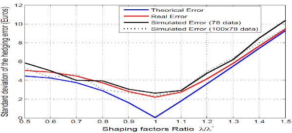
(a) $K=0,8X_{T}$

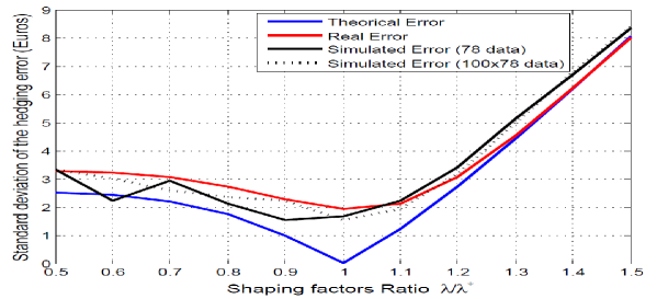
(b) $K=X_{T}$

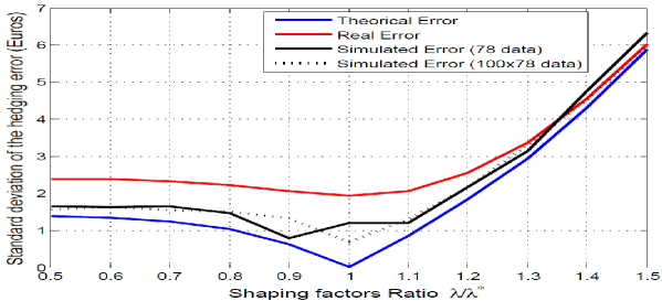
(c) $K=1.2X_{T}$

Figure 1: Standard deviation of the hedging error as a function of the ratio between the shaping factor used in the hedging strategy $\lambda$ and the real shaping factor $\lambda^{*}$ impacting the historical scenarios.

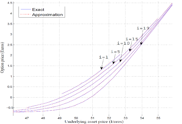
(a) Value function $x\mapsto u_{s}(x)$ with $p=0.1$ Euros and time steps $i=\in\{1,5,10,15,19\}$.

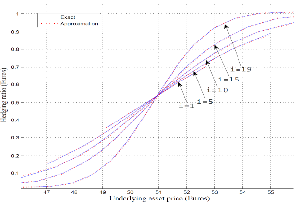
(b) Optimal strategy $x\mapsto\nu(t,x,p)$ for $p=0.1$ Euros and time steps $i\in\{1,5,10,15,19\}$.

Figure 2: Comparison between the numerical solution and the explicit formula.

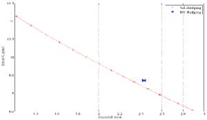
(a) $K=0,85X(t_{0})$

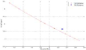
(b) $K=0,90X(t_{0})$

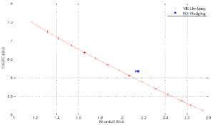
(c) $K=0,95X(t_{0})$

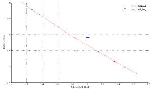
(d) $K=X(t_{0})$

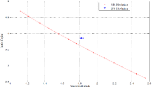
(e) $K=1,05X(t_{0})$

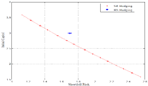
(f) $K=1,10X(t_{0})$

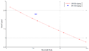
(g) $K=1,15X(t_{0})$

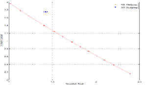
(h) $K=1,15X(t_{0})$

Figure 3: Initial capital w.r.t. the associated Shortfall Risk of the Black-Scholes strategy (blue) and the Shortfall strategy (red) with 95 % confidence interval (in dotted lines).

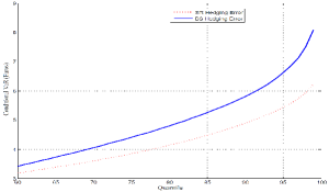
(a) $K=0,85X(t_{0})$

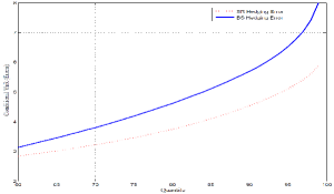
(b) $K=0,90X(t_{0})$

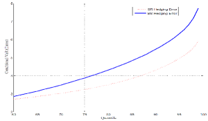
(c) $K=0,95X(t_{0})$

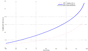
(d) $K=X(t_{0})$

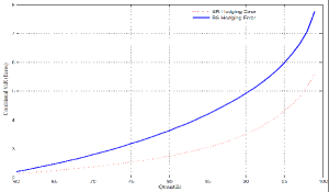
(e) $K=1,05X(t_{0})$

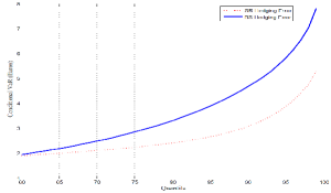
(f) $K=1,10X(t_{0})$

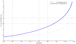
(g) $K=1,15X(t_{0})$

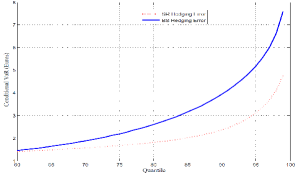
(h) $K=1,15X(t_{0})$

Figure 4: CVaR value w.r.t. the quantile level of the the strategies BS (blue) and SR (red).

Appendix: Geometric Dynamic Principle and HJB equation

In what follows, we put ourselves in the Brownian filtration setting of [21] and [5], which encompasses our framework. We omit the presence of $\Lambda$ by assuming $\mathbb{P}\left[{\Lambda=1}\right]=1$ and place ourselves on the interval $[0,T^{*}]$. We provide one side of the GDP used to derive the supersolution property.

Theorem 1 (Th 3.1, [21]).

Fix $(t,x,p,y)\in{\mathbf{S}}\times[-\kappa,\infty)$ such that $y>V(t,x,p)$ and a family of stopping times $\left\{\theta^{\nu,\alpha}\leavevmode\nobreak\ :\leavevmode\nobreak\ (\nu,\alpha)\in{\cal U}_{t,y}\times{\cal A}_{t,p}\right\}$. Then there exists $(\nu,\alpha)\in{\cal U}_{t,y}\times{\cal A}_{t,p}$ such that

$$Y^{t,x,y,\nu}_{\theta^{\nu,\alpha}}\geq V(\theta^{\nu,\alpha},X^{t,x}_{\theta^{\nu,\alpha}},P_{\theta^{\nu,\alpha}}^{t,p,\alpha})\ \mathbb{P}-\mbox{a.s.}$$

and $Y^{t,x,y,\nu}_{s\wedge\theta^{\nu,\alpha}}\geq-\kappa$ for all $s\in[t,T^{*}]$ $\mathbb{P}-\mbox{a.s.}$

Let $V_{*}$ be defined by $V_{*}(t,x,p):=\liminf\left\{V(t^{\prime},x^{\prime},p^{\prime})\leavevmode\nobreak\ :\leavevmode\nobreak\ B\ni(t^{\prime},x^{\prime},p^{\prime})\to(t,x,p)\right\}$ where $B$ denotes an open subset of $[0,T^{*}]\times{\mathbb{R}}^{*}_{+}\times{\mathbb{R}}^{*}_{-}$ with $(t,x,p)\in{\rm cl}(B)$. We assume that $V$ is locally bounded on ${\mathbf{S}}$, so that $V_{*}$ is finite. In what follows, we introduce only the supersolution property for $V_{*}$, deriving from Theorem 1, in the special case given by dynamics (1),(3) and (11).

For $\varepsilon\geq 0$, we introduce the relaxed operator $\Theta\mapsto\bar{F}_{\varepsilon}(\Theta)$ for the variable

$$\Theta=(t,x,p,d,d_{x},d_{p},d_{xx},d_{pp},d_{xp})\in{\mathbf{S}}\times{\mathbb{R}}^{6}$$

given by

$$\bar{F}_{\varepsilon}(\Theta):=\sup\limits_{(u,a)\in{\cal N}_{\varepsilon}(\Theta)}\left\{\left(u-d_{x}\right)\mu(t,x)-\frac{1}{2}\left(\sigma^{2}(t,x)d_{xx}+a^{2}p^{2}d_{pp}+2ap\sigma(t,x)d_{xp}\right)\right\}$$ (63)

with

$${\cal N}_{\varepsilon}(\Theta):=\left\{(u,a)\in{\mathbb{R}}^{2}\leavevmode\nobreak\ :\leavevmode\nobreak\ \left|\sigma(t,x)\left(u-d_{x}\right)-apd_{p}\right|\leq\varepsilon\right\}\;.$$ (64)

to finally introduce $\bar{F}^{*}(\Theta):=\limsup\left\{\bar{F}_{\varepsilon}(\Theta^{\prime})\leavevmode\nobreak\ :\leavevmode\nobreak\ \varepsilon\searrow 0,\Theta^{\prime}\rightarrow\Theta\right\}$. We adopt the convention $\sup\emptyset=-\infty$ and

$$\bar{F}^{*}\varphi=\bar{F}^{*}(t,x,p,\varphi(x,p),\varphi_{x}(t,x),\varphi_{p}(t,x),\varphi_{xx}(t,x),\varphi_{pp}(t,x),\varphi_{xp}(t,x))$$

for a smooth function $\varphi$. We hence formulate the supersolution property of $V_{*}$. For definitions and use of viscosity solutions, we refer to [11]. The supersolution property inside the domain is given by Theorem 2.1 and Corollary 3.1 in [5]. The boundary condition at $t=T^{*}$ is given by Theorem 2.2 in [5]. In our case, by assuming the concavity of $\Psi$ in $y$, we have the convexity of $\Psi^{-1}$ in the $p$ variable. We also have ${\cal N}_{0}(\Theta)\neq\emptyset$ for any $\Theta$. According to these two properties, the terminal condition takes a much more simple form. Altogether, we obtain the following.

Theorem 2 (Th. 2.1-2.2, [5]).

The function $V_{*}$ is a viscosity supersolution of

$$\left\{\begin{array}[]{ll}-\varphi_{t}(t,x,p)+\bar{F}^{*}\varphi(t,x,p)=0&\text{on }[0,T^{*})\times{\mathbb{R}}^{*}_{+}\times{\mathbb{R}}^{*}_{-}\\ V_{*}(T,x,p)\geq\Psi^{-1}(x,p)&\text{on }{\mathbb{R}}^{*}_{+}\times{\mathbb{R}}^{*}_{-}\end{array}\right.\;.$$ (65)

There is a special Cauchy boundary problem for $p=0$ we elude here. In our case, since $\Psi(0)=0$, the stochastic target problem reduces to the superhedging problem. The target must be reached ${\mathbb{P}}$-almost surely and we obtain directly the HJB equation of [21]. In our complete market framework, it straightly provides the Black-Scholes equation (24) to which $V_{*}(.,0)$ is also a viscosity solution.

References

- [1] Becherer, D. Rational hedging and valuation with utility-based preferences Universitätsbibliothek, Technischen Universität Berlin, 2001.
- [2] Benth, F. and Koekebakker, S. Stochastic modeling of financial electricity contracts. Journal of Energy Economics, 30, 1116-1157, 2007.
- [3] Bouchard, B. and Dang, N. Generalized stochastic target problems for pricing and partial hedging under loss constraints -Application in optimal book liquidation. Finance and Stochastics, 17(1), 31–72, 2011.
- [4] Bouchard, B. and Dang, N. Optimal Control versus Stochastic Target problems: An Equivalence Result. Systems & Control Letters, 61 (2), 343–346, 2012.
- [5] Bouchard, B., Elie, R and Touzi, N. Stochastic target problems with controlled loss. SIAM Journal on Control and Optimization, 48, 3123–3150, 2009.
- [6] Bouchard, B., Moreau, L. and Nutz, M. Stochastic target games with controlled loss. arXiv preprint arXiv:1206.6325. 2012.
- [7] Bouchard, B., Moreau, L., and Soner, M. H. Hedging under an expected loss constraint with small transaction costs. arXiv preprint arXiv:1309.4916. 2013.
- [8] Bouchard, B. and Nutz, M. Weak dynamic programming for generalized state constraints. SIAM Journal on Control and Optimization, 50(6), 3344–3373, 2012.
- [9] Bouchard, B. and Vu, T. The obstacle version of the geometric dynamic programming principle: Application to the pricing of american options under constraints. Applied Mathematics & Optimization, 61, 235–265, Springer, 2010.
- [10] Broadie, M. and Glasserman, P. Estimating security price derivatives using simulation. Management science, JSTOR, 269–285, 1996.
- [11] Crandall, M. G., Ishii, H. and Lions, P. L. User’s guide to viscosity solutions of second order partial differential equations. Bulletin of the American Mathematical Society, 27(1), 1–67, 1992.
- [12] Cvitanic, J. Minimizing expected loss of hedging in incomplete and constrained markets. SIAM Journal on Control and Optimization, 38(4), 1050–1066, 2000.
- [13] Eichhorn, A., Romisch, W. and Wegner, I. Mean-risk optimization of electricity portfolios using multiperiod polyhedral risk measures. Power Tech, 2005 IEEE Russia, 1–7, 2005.
- [14] Föllmer, H. and Leukert, P. Quantile hedging. Finance and Stochastics, 3(3), 251–273, 1999.
- [15] Föllmer, H. and Leukert, P. Efficient hedging: cost versus shortfall risk. Finance and Stochastics, 4, 117–146, 2000.
- [16] Föllmer, H. and Penner, I. Convex risk measures and the dynamics of their penalty functions. Statistics & Decisions, Oldenbourg Wissenschaftsverlag GmbH, 24, 61–96, 2006.
- [17] Janson, S. and Tysk, J. Feynman-Kac formulas for Black-Scholes type operators. Bull. London Math. Soc., 38 (2), 262–289, 2006.
- [18] Lindell, A. and Raab, M. Strips of hourly power options–Approximate hedging using average-based forward contracts. Energy Economics, Elsevier, 31, 348–355, 2009.
- [19] Moreau, L. Stochastic target problems with controlled loss in jump diffusion models. SIAM Journal on Control and Optimization, 49, 2577–2607, 2011.
- [20] Soner, H. and Touzi, N. Dynamic programming for stochastic target problems and geometric flows. Journal of the European Mathematical Society, 4, 201–236, Springer, 2002.
- [21] Soner, H Mete and Touzi, Nizar. Stochastic target problems, dynamic programming, and viscosity solutions. SIAM Journal on Control and Optimization, 41(2), 404–424, 2002.
- [22] Verschuere, M. and Von Grafenstein, L. Futures hedging in power markets: Evidence from the EEX. Working paper, 2003.