On the similarity of meshless discretizations of Peridynamics and Smooth-Particle Hydrodynamics

Abstract

This paper discusses the similarity of meshless discretizations of Peridynamics and Smooth-Particle-Hydrodynamics (SPH), if Peridynamics is applied to classical material models based on the deformation gradient. We show that the discretized equations of both methods coincide if nodal integration is used. This equivalence implies that Peridynamics reduces to an old meshless method and all instability problems of collocation-type particle methods apply. These instabilities arise as a consequence of the nodal integration scheme, which causes rank-deficiency and leads to spurious zero-energy modes. As a result of the demonstrated equivalence to SPH, enhanced implementations of Peridynamics should employ more accurate integration schemes.

1 Introduction

The Peridynamic theory, originally devised by Silling [1], is a nonlocal extension of classical continuum mechanics, which is based on partial differential equations. Since partial derivatives do not exist on crack surfaces and other singularities, the classical equations of continuum mechanics cannot be applied directly when such features are present. In contrast, the Peridynamic balance of linear momentum is formulated as an integral equation, which remains valid in the presence of material discontinuities. Therefore, the Peridynamic theory can be applied directly to modelling both bulk and interface properties, using the same mathematical model. Additionally, Peridynamics is readily implemented in a meshless formulation, which facilitates the simulation of large deformations when compared to the traditional mesh-based Finite-Element method used for simulating solid mechanics in the classical continuum theory [2].

With these desirable features, Peridynamics has received considerable attention by researchers interested in numerically describing fundamental crack growth and failure effects in brittle materials [3, 4, 5, 6]. However, the scope of the original Peridynamic formulation included only so-called bond-based models [7] which were limited to a fixed Poisson ratio for linear isotropic materials and could not describe true plastic yielding. Further development of the theory led to state-based models [8], which can, in principle, describe all classic material behaviour. In particular, the state-based theory offers a route to approximating the classical deformation gradient, which can be used to obtain a classical stress tensor. The stress tensor can then be converted into nodal forces using a Peridynamic integral equation. This promising situation, i.e., the ability to use classical material models with a method that remains valid at material discontinuities, has prompted a number of studies where plastic yielding, damage, and failure was simulated using this new meshless method [9, 10].

However, there exists a demand for studies which compare Peridynamics to other meshless methods. While the theoretical correspondence of Peridynamics with classical elasticity theory has been established [11], no information is available on the accuracy of the discretized Peridynamic expression suitable for computer implementation. Relevant questions that need to be addressed include, but are not limit to, whether linear fields can be exactly reproduced by the discretized theory, and what the the order of convergence is when Peridynamic solutions are compared against exact results. Little is known about how common problems encountered with other meshless methods, e.g., the tensile instability [12] or the rank deficiency problem [13] affect Peridynamics. As an exception to this general observation, Bessa et al [14] have published a study which demonstrates the equivalence of state-based Peridynamics and the reproducing Kernel Particle Method (RKPM), if nodal integration is used. However, no published studies are available to the best of this author’s knowledge, which compare Peridynamics to other meshless methods.

The goal of our paper is to elucidate on some properties of Peridynamics with respect to other meshless methods. In particular, we establish that the discrete equations of the Peridynamic formulation using classical material models is identical to a very well-known meshless technique: Smooth Particle Hydrodynamics (SPH) in the Total-Lagrangian formulation. This equivalence facilitates understanding of Peridynamics using the large body of literature already published for other meshless methods, see e.g. [15] and [16]. The key observations of our work address two issues: (i) Discretizations of Peridynamics directly arrive at correct equations which conserve linear and angular momentum. These features can only be obtained in SPH by assuming ad hoc corrections such as explicict symmetrization. (ii) All of the problems that apply to collocation-type particle methods also apply to Peridynamics if this theory is discretized using nodal integration.

The remainder of this paper is organized as follows: we begin by deriving the fundamental expressions of the SPH approximation including the most important corrections for this method, which allow it to be used with the minimal level of accuracy required for solid mechanics simulations. Then, the essential Peridynamic expressions required for simulating classical material models are derived. Building on this foundation, the equivalence of SPH and this particular variant of Peridynamics is shown. Finally, the implications of this observation are discussed and Peridynamics (with classical material models) is characterized using the established terminology encountered in the SPH literature.

2 Total Lagrangian SPH

Smooth Particle Hydrodynamics [17] was originally devised as a Lagrangian particle method with the smoothing kernel moving with the particle, thus redefining the interaction neighbourhood for every new position the particle attains. In this sense, the kernel of the original SPH formulation has Eulerian character, as other particles move through the interaction neighbourhood. The tensile instability [12] encountered in SPH, where particles clump together under negative pressure conditions, has been found to be caused by the Eulerian kernel functions [13]. Consequently, Total Lagrangian formulations were developed [18, 19, 20], which use a constant reference configuration for defining the interaction neighborhood of the particles. see Typically, the initial, undeformed configuration is taken for this purpose. In the following, this concept and the associated nomenclature is briefly explained with the limited scope of obtaining SPH expressions that are to be compared with the Peridynamic expressions. For a more detailed derivation, the reader is referred to the works cited above.

2.1 Total Lagrangian formulation

In the total Lagrangian formulation, conservation and constitutive equations are expressed in terms of the material coordinates $\bm{X}$, which are taken to be the coordinates of the initial, undeformed reference configuration. A mapping between the current coordinates, and the reference coordinates describes the body motion at time $t$:

$$\bm{x}=\phi(\bm{X},t),$$ (1)

Here, $\bm{x}$ are the current, deformed coordinates and $\bm{X}$ the reference (Lagrangian) coordinates. The displacement $\bm{u}$ is given by

$$\bm{u}=\bm{x}-\bm{X},$$ (2)

The conservation equations for mass, impulse, and energy in the total Lagrangian formulation are given by

$$\rho J=\rho_{0}J_{0}$$ (3)

$$\ddot{u}=\frac{1}{\rho_{0}}\bm{\nabla}_{0}\cdot\bm{P}$$ (4)

$$\dot{e}=\frac{1}{\rho_{0}}\dot{\bm{F}}:\bm{P}^{T},$$ (5)

where $J$ and $J_{0}$ are the current and initial Jacobian determinants. $\rho$ is the current mass density and $\rho_{0}$ is the initial mass density, $\bm{P}$ is the nominal stress tensor (the transpose of the first Piola-Kirchhoff stress tensor), $e$ is the internal energy, $\bm{\nabla}_{0}$ is the gradient or divergence operator expressed in the material coordinates, and $\bm{F}$ denotes the deformation gradient,

$$\bm{F}=\frac{\mathrm{d}\bm{x}}{\mathrm{d}\bm{X}}=\frac{\mathrm{d}\bm{u}}{\mathrm{d}\bm{X}}+\bm{I},$$ (6)

2.2 The SPH Approximation

The SPH approximation for a scalar function $f$ in terms of the Lagrangian coordinates can be written as

$$f(\bm{X_{i}})=\sum\limits_{j\in\mathcal{S}}V_{j}^{0}f(\bm{X_{j}})W_{i}\left(X_{ij}\right)$$ (7)

The sum extends over all particles within the range of a scalar weight function $W_{i}$, which is centered at position $\bm{X_{i}}$ and depends on the distance between coordinates $\bm{X}_{i}$ and $\bm{X}_{j}$, $X_{ij}=\lVert\bm{X_{j}}-\bm{X_{i}}\rVert$. $V^{0}$ is the volume associated with a particle in the reference configuration. The weight function is typically chosen to be radially symmetric and have compact support, i.e., it includes only neighbors within a certain radial distance. This domain of influence is denoted $S$.

The SPH approximation of a derivative of $f$ is obtained by operating directly with the gradient operator on the kernel functions,

$$\bm{\nabla}f(\bm{X_{i}})=\sum\limits_{j\in\mathcal{S}}V_{j}^{0}f(\bm{X_{j}})\bm{\nabla}W_{i}\left(X_{ij}\right),$$ (8)

where the gradient of the kernel function is defined as follows:

$$\bm{\nabla}W_{i}(X_{ij})=\left(\frac{\mathrm{d}W(X_{ij})}{\mathrm{d}X_{ij}}\right)\frac{\bm{X}_{j}-\bm{X}_{i}}{X_{ij}}$$ (9)

The conditions for the zeroth- and first-order completeness of the SPH approximation are stated as follows:

$$\sum\limits_{j\in\mathcal{S}}V_{j}^{0}W_{i}\left(X_{ij}\right)=1$$ (10)

$$\sum\limits_{j\in\mathcal{S}}V_{j}^{0}\bm{\nabla}W_{i}\left(X_{ij}\right)=0$$ (11)

In the simple form as stated here, neither of the completeness conditions are fulfilled by the SPH approximation. An ad-hoc improvement consists in adding eqn. (11) to eqn. 8, such that a symmetrized approximation for the derivative of a function is obtained,

$$\bm{\nabla}f(\bm{X_{i}})=\sum\limits_{j\in\mathcal{S}}V_{j}^{0}\left(f(\bm{X_{j}})-f(\bm{X_{i}})\right)\bm{\nabla}W_{i}\left(X_{ij}\right)$$ (12)

The symmetrization does not result in first-order completeness, however, it yields zeroth-order completeness for the derivatives of a function.

2.3 Restoring First-Order Completeness

In order to fulfill first-order completeness, the SPH approximation has to reproduce the constant gradient of a linear field. A number of correction techniques [21, 22, 23] exploit this condition as the basis for correcting the gradient of the SPH weight function,

$$\sum\limits_{j\in\mathcal{S}}V_{j}^{0}(\bm{X}_{j}-\bm{X_{i}})\otimes\bm{\nabla}W_{i}(X_{ij})\overset{!}{=}\bm{I},$$ (13)

where $\bm{I}$ is the diagonal unit matrix. Based on this expression, a corrected kernel gradient can be defined:

$$\tilde{\bm{\nabla}}W_{i}(X_{ij})=\bm{L}_{i}^{-1}\bm{\nabla}W_{i}(X_{ij}),$$ (14)

which uses the correction matrix $\bm{L}$, defined as:

$$\bm{L}_{i}=\sum\limits_{j\in\mathcal{S}}V_{j}^{0}\bm{\nabla}W_{i}(X_{ij})\otimes(\bm{X}_{j}-\bm{X_{i}}).$$ (15)

By construction, the corrected kernel gradient now satisfies eqn. (13),

$$\sum\limits_{j\in\mathcal{S}}V_{j}^{0}(\bm{X}_{j}-\bm{X_{i}})\otimes\bm{L}_{i}^{-1}\bm{\nabla}W_{i}(X_{ij})=\bm{I},$$ (16)

2.4 Corrected SPH expressions for Solid Mechanics

For calculating the internal forces of a solid body subjected to a deformation, expressions are required for (i) the deformation gradient, (ii) a constitutive equation which provides a stress tensor as function of the deformation gradient, and (iii) an expression for transforming the stresses into forces acting on the nodes which serve as the discrete representation of the body.

The deformation gradient is obtained by calculating the derivative of the displacement field, i.e., by using the symmetrized SPH derivative approximation, eqn. (12), for eqn. (6):

$$\bm{F}_{i}^{SPH}=\sum\limits_{j\in\mathcal{S}}V_{j}^{0}(\bm{u}_{j}-\bm{u_{i}})\otimes\bm{L}_{i}^{-1}\bm{\nabla}W_{i}(X_{ij})+\bm{I}.$$ (17)

Note that in the above equation, the corrected kernel gradient has been introduced via the matrix $\bm{L}_{i}^{-1}$. The SPH approximation of the stress divergence, eqn. (4), is not so clear. Depending on how it is performed, several different approximations can be obtained [24]. The most frequently used form, which is variationally consistent with respect to an energy minimization principle [22], is the following:

$$\bm{f}_{i}=\sum\limits_{j\in\mathcal{S}}V_{i}^{0}V_{j}^{0}\left(\bm{P}_{j}+\bm{P}_{i}\right)\bm{\nabla}W_{i}(X_{ij}).$$ (18)

For a radially symmetric kernel which depends only on distance, the antisymmetry property $\bm{\nabla}W_{i}(X_{ij})=-\bm{\nabla}W_{j}(X_{ji})$ holds. Therefore, the above force expression will conserve linear momentum exactly, as $\bm{f}_{ij}=-\bm{f}_{ji}$. We use the antisymmetry property of the kernel gradient to rewrite the force approximation as follows:

$$\bm{f}_{i} = \sum\limits_{j\in\mathcal{S}}V_{i}^{0}V_{j}^{0}\left(\bm{P}_{i}\bm{\nabla}W_{i}(X_{ij})+\bm{P}_{j}\bm{\nabla}W_{i}(X_{ij})\right)$$ (19)

$$= \sum\limits_{j\in\mathcal{S}}V_{i}^{0}V_{j}^{0}\left(\bm{P}_{i}\bm{\nabla}W_{i}(X_{ij})-\bm{P}_{j}\bm{\nabla}W_{j}(X_{ji})\right).$$ (20)

Replacing the uncorrected kernel gradient with the corrected gradient (c.f. eqn. (14), the following expression is obtained:

$$\bm{f}_{i}=\sum\limits_{j\in\mathcal{S}}V_{i}^{0}V_{j}^{0}\left(\bm{P}_{i}\bm{L}_{i}^{-1}\bm{\nabla}W_{i}(X_{ij})-\bm{P}_{j}\bm{L}_{j}^{-1}\bm{\nabla}W_{j}(X_{ji})\right)$$ (21)

This corrected force evaluation conserves linear momentum due to its antisymmetry with respect to interchange of the particle indices $i$ and $j$, i.e., $\bm{f}_{ij}=-\bm{f}_{ji}$. The here constructed antisymmetric force expression is usually not seen in the literature. In contrast, it seems to be customary [21, 22, 23] to directly insert the corrected kernel gradient into eqn. (18), which destroys the local conservation of linear momentum. We note that the above construction of the SPH expression that conserves linear momentum is arbitrary, and in similar spirit to the ad-hoc symmetrization procedure encountered in eqn. (12).

3 Peridynamics for classical material models

This section provides a concise derivation of the Peridynamic approximation of the deformation gradient and the forces acting on particles. In contrast to the preceding section, where this quantities have been derived for SPH, we employ a different nomenclature here, which is consistent with the most relevant Peridynamic literature. In Peridynamics, each particle defines the origin of an influence domain, termed neighborhood $\mathcal{H}$, of radius $\delta$. Within this neighborhood, vectors $\bm{\xi}$ from the origin to any point in $\mathcal{H}$ exist, see the following figure.

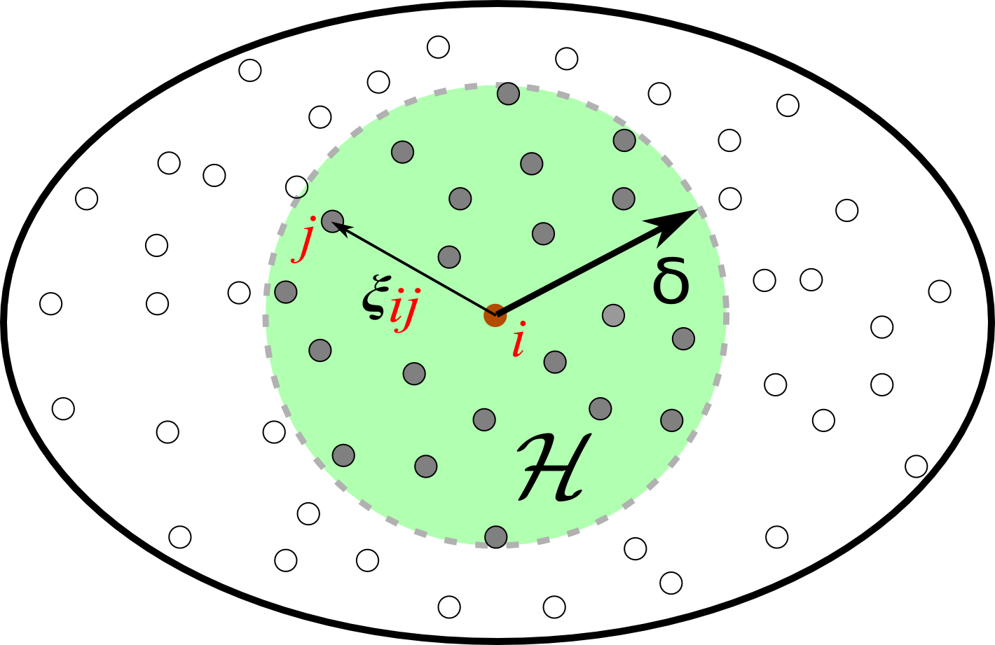
Figure 1: In the meshless Peridynamic method, particle interactions are defined in a reference configuration which is shown here. A region of influence termed $\mathcal{H}$ is defined by a radial cutoff $\delta$ around a particle $i$. Bonds exist between $i$ and all particles $j$ within $\mathcal{H}$. These bonds are denoted here by $\bm{\xi}_{ij}$, of which only one is shown above. Note that this representation already employs discrete particle locations whereas the Peridynamic theory assumes a continuum of points.

3.1 Vector states

Central to the state-based Peridynamic theory is the concept of states. States are functions that act on on vectors. This is written in the following way,

$$\underline{\bm{A}}\left<\bm{\xi}\right>=\bm{\xi}^{\prime},$$ (22)

where the state $\underline{\bm{A}}$ has acted on the vector $\bm{\xi}$ to produce a different vector $\bm{\xi}^{\prime}$. Angular brackets indicate which vector the state acts upon. The mapping results produce tensors of different order, depending on the nature of the state. Vector states of order one map a vector to a different vector. Scalar states of order zero produce a scalar for every vector they act on. For the purpose of this paper we only need to be concerned with the following states:

The reference position vector state $\underline{\bm{X}}$ returns the original bond vector.

$$\underline{\bm{X}}\left<\bm{\xi}\right>=\bm{\xi}\in\mathbb{R}^{3}$$ (23)

The deformation state $\underline{\bm{Y}}$ returns the deformed image of the original bond vector. Let the original vector go from $\bm{X}$ to $\bm{X^{\prime}}$, i.e., $\bm{\xi}=\bm{X^{\prime}}-\bm{X}$. Upon deformation, the coordinates of these two points change to $\bm{x}$ and $\bm{x^{\prime}}$. The deformation state vector returns the deformed image of the original vector, i.e.,

$$\underline{\bm{Y}}\left<\bm{\xi}\right>=\bm{x^{\prime}}-\bm{x}$$ (24)

The influence function $\underline{\omega}$ is a scalar state that returns a number $w$ that depends only on the magnitude of $\bm{\xi}$.

$$\underline{\omega}\left<\xi\right>=w\in\mathbb{R}^{+}$$ (25)

Vector and scalar states can be combined using the usual mathematical operations addition, subtraction, multiplication, etc. The conventions are detailed in [8]. Here, we only need the definition of the tensor product between two vector states $\underline{\bm{A}}$ and $\underline{\bm{B}}$,

$$\underline{\bm{A}}*\underline{\bm{B}}=\int\limits_{\mathcal{H}}\underline{\omega}\left<\xi\right>\underline{\bm{A}}\left<\bm{\xi}\right>\otimes\underline{\bm{B}}\left<\bm{\xi}\right>\mathrm{d}V_{\bm{\xi}}$$ (26)

This tensor product is required for the following Peridynamic concepts. Firstly, the shape tensor is defined:

$$\mathbf{K}=\underline{\bm{X}}*\underline{\bm{X}}=\int\limits_{\mathcal{H}}\underline{\omega}\left<\xi\right>\bm{\xi}\otimes\bm{\xi}\mathrm{d}V_{\bm{\xi}}$$ (27)

$\bm{K}$ is symmetric and real and thus positive-definite, implying that it can be inverted. The shape tensor is then used in the concept of tensor reduction, which is an operation that produces a second order tensor from two vector states:

$$\mathbf{C}=\left(\underline{\bm{A}}*\underline{\bm{B}}\right)\bm{K}^{-1}=\left(\int\limits_{\mathcal{H}}\underline{\omega}\left<\xi\right>\underline{\bm{A}}\left<\bm{\xi}\right>\otimes\underline{\bm{B}}\left<\bm{\xi}\right>\mathrm{d}V_{\bm{\xi}}\right)\bm{K}^{-1}$$ (28)

3.2 Calculation of the deformation gradient tensor in Peridynamics

The deformation gradient tensor may be approximated as a tensor reduction of deformation vector state and reference position vector state according to eqn. (134) in [8]:

$$\bm{F}\approx(\underline{\bm{Y}}*\underline{\bm{X}})\bm{K}^{-1}$$ (29)

The necessary Peridynamic calculus for evaluating this quantity has been presented above. We now make the transition from the continuum representation to a discrete nodal, or particle representation, converting integrals to sums. A piecewise constant discretization of the integrals defined above yields the discrete shape tensor as

$$\bm{K}_{i}=\sum\limits_{j\in\mathcal{H}_{i}}V_{j}^{0}\underline{\omega}\left<\xi_{ij}\right>\bm{\xi}_{ij}\otimes\bm{\xi}_{ij}$$ (30)

Here, the sum includes all particles $j$ within the neighborhood $\mathcal{H}_{i}$ of $i$ and $V_{j}^{0}$ is the volume of particle $j$. The discrete expression for the approximate deformation gradient is obtained as:

$$\bm{F}_{i}^{PD}=\left(\sum\limits_{j\in\mathcal{H}_{i}}V_{j}^{0}\underline{\omega}\left<\xi_{ij}\right>\bm{x}_{ij}\otimes\bm{\xi}_{ij}\right)\bm{K}_{i}^{-1}=\left(\sum\limits_{j\in\mathcal{H}_{i}}V_{j}^{0}\underline{\omega}\left<\xi_{ij}\right>\bm{u}_{ij}\otimes\bm{\xi}_{ij}\right)\bm{K}_{i}^{-1}+\bm{I}$$ (31)

3.3 The Peridynamic force expression obtained from a classical stress tensor

The fundamental equation of Peridynamics is an integral equation of force densities (force per volume) which ensures local conservation of impulse, see eqn. (28). in [8]:

$$\bm{f}^{PD}=V_{\bm{X}}\int\limits_{\mathcal{H}_{X}}\left\{\underline{\bm{T}}[\bm{X}]\left<\bm{X}^{\prime}-\bm{X}\right>-\underline{\bm{T}}[\bm{X}^{\prime}]\left<\bm{X}-\bm{X^{\prime}}\right>\right\}\mathrm{d}V_{X^{\prime}}$$ (32)

Here, $\bm{T}[\bm{X}]$ is a vector state, which operates on the bond $\bm{\xi}=\bm{X}^{\prime}-\bm{X}$ in order to yield a contribution to the force density at $\bm{X}$. The antisymmetric counterpart $\bm{T}[\bm{X}^{\prime}]$ ensures balance of linear momentum and $V_{\bm{X}}$ is the volume associated with the coordinate $\bm{X}$. The vector state $\bm{T}$ is related the classical stress tensor, which can be computed using the deformation gradient and a classical material model. Specifically, this relation is stated as follows, see eqn. (142). in [8]:

$$\underline{\bm{T}}[\bm{X}]\left<\bm{\xi}\right>=\underline{\omega}\left<\xi\right>\bm{P}_{\bm{X}}\bm{K}^{-1}_{\bm{X}}\bm{\xi}$$ (33)

The stress tensor $\bm{P}$ above is the nominal stress tensor which applies here as the stress is expressed in the reference configuration. The dependence on $\bm{X}$ signifies that both stress and shape tensor have to be evaluated at coordinate $\bm{X}$. Converting to a discrete particle expression, one obtains:

$$\bm{f}_{i}^{PD} = \sum\limits_{j\in\mathcal{H}_{i}}V_{i}^{0}V_{j}^{0}\left\{\underline{\bm{T}}_{i}\left<\bm{\xi}_{ij}\right>-\underline{\bm{T}}_{j}\left<\bm{\xi}_{ji}\right>\right\}$$ (34)

$$= \sum\limits_{j\in\mathcal{H}_{i}}V_{i}^{0}V_{j}^{0}\left\{\underline{\omega}\left<\xi_{ij}\right>\bm{P}_{i}\bm{K}_{i}^{-1}\bm{\xi}_{ij}-\underline{\omega}\left<\xi_{ji}\right>\bm{P}_{j}\bm{K}_{j}^{-1}\bm{\xi}_{ji}\right\}$$ (35)

4 The Correspondence between Peridynamic and SPH expressions for deformation gradient and particle forces

The discrete Peridynamic approximation of both the deformation gradient and the particle forces arising from a classical stress tensor are equal to the Total-Lagrangian SPH expressions with linear kernel gradient correction. In order to show this equivalence, we introduce some changes in nomenclature:

$$\mathcal{H}_{i} = S_{i}$$ (36)

$$\bm{\xi}_{ij} = \bm{X}_{ij}$$ (37)

$$\underline{\omega}\left<\xi_{ij}\right> = \frac{1}{X_{ij}}\frac{\mathrm{d}W(X_{ij})}{\mathrm{d}X_{ij}}.$$ (38)

Note that the postulated equivalence in the last line above states that the derivative of the SPH weight function has to equal the Peridynamic weight function. However, no implications arise from this requirement, as suitable weight functions can be chosen which fulfills this requirement.

4.1 Equality of shape tensor and first-order correction matrix

With these changes, the Peridynamic shape tensor becomes equal to the correction matrix required for first-order consistent SPH:

$$\bm{K}_{i} = \sum\limits_{j\in\mathcal{H}_{i}}V_{j}^{0}\underline{\omega}\left<\xi_{ij}\right>\bm{\xi}_{ij}\otimes\bm{\xi}_{ij}$$ (39)

$$= \sum\limits_{j\in\mathcal{S}_{i}}V_{j}^{0}\frac{1}{X_{ij}}\frac{\mathrm{d}W(X_{ij})}{\mathrm{d}X_{ij}}\bm{X}_{ij}\otimes\bm{X}_{ij}$$ (40)

$$= \sum\limits_{j\in\mathcal{S}_{i}}V_{j}^{0}\bm{\nabla}W_{i}(X_{ij})\otimes(\bm{X}_{j}-\bm{X_{i}})$$

$$\therefore$$

$$\bm{K}_{i} = \bm{L}_{i}$$ (42)

4.2 Equality of the deformation gradient

In a similar manner, the Peridynamic expression of the deformation gradient can be shown to be equal to the SPH approximation:

$$\bm{F}_{i}^{PD} = \left(\sum\limits_{j\in\mathcal{H}_{i}}V_{j}^{0}\underline{\omega}\left<\xi_{ij}\right>\bm{u}_{ij}\otimes\bm{\xi}_{ij}\right)\bm{K}_{i}^{-1}+\bm{I}$$ (43)

$$= \left(\sum\limits_{j\in\mathcal{S}}V_{j}^{0}\frac{1}{X_{ij}}\frac{\mathrm{d}W(X_{ij})}{\mathrm{d}X_{ij}}\bm{u}_{ij}\otimes\bm{X}_{ij}\right)\bm{L}_{i}^{-1}+\bm{I}$$ (44)

$$= \sum\limits_{j\in\mathcal{S}}V_{j}^{0}\bm{u}_{ij}\otimes\left(\bm{L}_{i}^{-1}\frac{1}{X_{ij}}\frac{\mathrm{d}W(X_{ij})}{\mathrm{d}X_{ij}}\bm{X}_{ij}\right)+\bm{I}$$

$$\therefore$$

$$\bm{F}_{i}^{PD} = \bm{F}_{i}^{SPH}$$ (46)

Thus, the Peridynamic concept of reduction leads to the approximation of a tensor field, which is correct to first order.

4.3 Equality of particle forces

Using the same rules for changing the Peridynamic notation into SPH notation, one obtains from the Peridynamic force expression:

$$\bm{f}_{i}^{PD} = \sum\limits_{j\in\mathcal{H}}V_{i}^{0}V_{j}^{0}\left\{\underline{\omega}\left<\xi_{ij}\right>\bm{P}_{i}\bm{K}_{i}^{-1}\bm{\xi}_{ij}-\underline{\omega}\left<\xi_{ji}\right>\bm{P}_{j}\bm{K}_{j}^{-1}\bm{\xi}_{ji}\right\}$$ (47)

$$= \sum\limits_{j\in\mathcal{S}}V_{i}^{0}V_{j}^{0}\left\{\frac{1}{X_{ij}}\frac{\mathrm{d}W(X_{ij})}{\mathrm{d}X_{ij}}\bm{P}_{i}\bm{L}_{i}^{-1}\bm{X}_{ij}-\frac{1}{X_{ji}}\frac{\mathrm{d}W(X_{ji})}{\mathrm{d}X_{ji}}\bm{P}_{j}\bm{L}_{j}^{-1}\bm{X}_{ji}\right\}$$ (48)

$$= \sum\limits_{j\in\mathcal{S}}V_{i}^{0}V_{j}^{0}\left\{\bm{P}_{i}\bm{L}_{i}^{-1}\bm{\nabla}W_{i}(X_{ij})-\bm{P}_{j}\bm{L}_{j}^{-1}\bm{\nabla}W_{j}(X_{ji})\right\}$$

$$\therefore$$

$$\bm{f}_{i}^{PD} = \bm{f}_{i}^{SPH}$$ (50)

5 Implementation and numerical results

5.1 Implementation issues

The equality of Total-Lagrangian SPH and Peridynamic for classical material models with nodal integration raises some advantageous implementation issues. The first point concerns the weight function and its derivative, which is usually attributed great influence in SPH. In contrast, Peridynamic implementations typically use a constant unit weight function, i.e., $\xi_{ij}=1\,\forall\,j\,\in\mathcal{H}_{i}$. Using the Peridynamics to SPH translation, eqn. (38), this corresponds to a constant gradient for the SPH scheme. Such a constant implies that the associated weight function is apparently not a proper SPH weight function, i.e., it is certainly not normalized: $\int_{S}1\mathrm{d}V\neq 1$. This apparent contradiction is solved by the first-order correction scheme used here: The ansatz used for deriving the corrected gradient, eqn. (14) does not depend on any normalization factor as the multiplication the matrix inverse of $\bm{L}$ cancels any constant factor in the weight function. In fact, it can be shown that this route to a corrected kernel gradient represents a Moving Least Squares formulation with a linear basis [25, 26]. It can be concluded that the weight function (or indeed its derivative) can be chosen quite arbitrarily within this scheme. For the purpose of illustrating an implementation of the first-order corrected scheme, the uncorrected kernel gradient is simply defined as $W_{ij}\bm{X}_{ij}$. Algorithm 1 outlines an efficient implementation which moves the multiplication with the shape matrix outside of the inner loop (loop over neighbors $j$ of particle $i$), in order to save unnecessary calculations.

Algorithm 1 First-order corrected SPH or deformation-gradient based Peridynamics with nodal integration. Note that the constitutive law used here is expressed using the Green-Lagrange strain and the Lamé parameters $\lambda$ and $\mu$.

1:for all $i$ do

2:     $\bm{F}_{i}\leftarrow\bm{0}$ $\triangleright$ zero deformation gradient

3:     $\bm{L}_{i}\leftarrow\bm{0}$ $\triangleright$ zero shape matrix

4:     $\bm{f}_{i}\leftarrow\bm{0}$ $\triangleright$ zero force

5:

6:     for all $j\in\mathcal{S}_{i}$ do $\triangleright$ first loop over pairs $(i,j)$

7:         $\triangleright$ note that $W_{ij}\bm{X}_{ij}$ replaces the usual SPH kernel gradient

8:         $\bm{F}_{i}\leftarrow\bm{F}_{i}+V_{j}^{0}W_{ij}\bm{x}_{ij}\otimes\bm{X}_{ij}$ $\triangleright$ sum deformation gradient

9:         $\bm{L}_{i}\leftarrow\bm{L}_{i}+V_{j}^{0}W_{ij}\bm{X}_{ij}\otimes\bm{X}_{ij}$ $\triangleright$ sum shape matrix

10:     end for

11:

12:     $\bm{L}_{i}\leftarrow\bm{L}_{i}^{-1}$ $\triangleright$ invert shape matrix

13:     $\bm{F}_{i}\leftarrow\bm{F}_{i}\bm{L}_{i}$ $\triangleright$ compute corrected deformation gradient

14:

15:     $\triangleright$ compute stress using linear-elastic constitutive law

16:     $\bm{E}_{i}\leftarrow\frac{1}{2}\left(\bm{F}_{i}^{T}\bm{F}_{i}-\bm{I}\right)$ $\triangleright$ Green-Lagrange strain

17:     $\bm{S}_{i}\leftarrow\lambda\mathrm{Tr}\{\bm{E}_{i}\}+2\mu\bm{E}_{i}$ $\triangleright$ $2^{nd}$ Piola-Kirchhoff stress

18:     $\bm{P}_{i}\leftarrow\bm{F}_{i}\bm{S}_{i}$ $\triangleright$ $1^{st}$ Piola-Kirchhoff stress

19:     $\bm{P}_{i}\leftarrow\bm{P}_{i}\bm{L}_{i}$ $\triangleright$ multiply stress tensor with shape matrix

20:

21:     for all $j\in\mathcal{S}_{i}$ do $\triangleright$ second loop over pairs $(i,j)$

22:         $\bm{f}_{i}\leftarrow\bm{f}_{i}+V_{i}^{0}V_{j}^{0}W_{ij}\left(\bm{P}_{i}+\bm{P}_{j}\right)\bm{X}_{ij}$ $\triangleright$ sum force

23:     end for$\triangleright$ move particle $i$ according to time integration scheme

24:end for

This algorithm exhibits two main features: A first loop over all pairs of interacting particles is required to define the shape matrix and deformation gradient. Naive implementations might split up this loop into two independent loops and first calculate only the shape matrix. However, as the kernel gradient correction depends only on the shape matrix of particle $i$, c.f. eqn. (17), these operations can be combined and the correct deformation gradient obtained by post-multiplying with the shape matrix. With the corrected deformation gradient at hand, a stress tensor is computed using the constitutive law. Here, a finite-strain theory is employed, which provides a linear relationship between strain and stress, based on the Lamé parameters $\lambda$ and $\mu$. The stress measure obtained this way is the Second Piola-Kirchhoff stress, which is applicable to the reference configuration. This stress measure is pushed forward to the current configuration (First Piola-Kirchhoff stress), as forces are applied to the current particle positions. The calculation of the forces requires a second loop over all pairs of interacting particles. To avoid multiplication of the kernel gradients with the shape matrix inside the second loop, the shape matrices are multiplied with the stress tensors before entering this loop. Once the forces are computed, the particle positions can updated according to any chosen time-integration scheme.

5.2 Numerical examples

The aim of this work is to show the equivalence of first-order corrected Total-Lagrangian SPH and Peridynamics applied to classical material models in combination with nodal integration. While the equivalence has been mathematically proven in sec. (4), it is also of interest to demonstrate the effects of the instability which emerges if nodal integrations used. To this end, the implementation according to Algorithm 1, in combination with a unit weight function and a leap-frog time integrator is used. For comparison purposes, reference solutions which do not suffer from rank-deficiency due to nodal integration are shown which are obtained using a meshfree code that employs a stabilization technique based on higher-order derivatives, similar to [27].

5.2.1 Patch test and stability

The patch test can be regarded as the most basic test for a solid mechanics simulation code. A strip of some material that is discretized using several elements (or SPH / Peridynamic particles) is subjected to a uniform strain field and the stress is computed. Regardless of the discretization, the stress should be uniform everywhere. SPH / Peridynamics with first-order corrected kernel gradients is well-known to pass this test. Here, however, we are interested in the subsequent time-integration following such an initial perturbation. To this end, a random initial particle configuration is obtained by discretizing a square patch of edge length 1 m and uniform area mass density $\rho=1\mathrm{kg/m^{2}}$ into 444 quadliteral area elements using a stochastic algorithm based on triangular Voronoi tesselation and recombination of the triangles into quadliterals. Particle volumes and masses are obtained from the quadliteral area and the prescribed mass density. The kernel radius is adjusted individually for each particle such that approximately 12 neighbors are within the kernel range. While the patch test can be easily simulated with an ordered initial configuration of particles, a non-uniform particle configuration poses extreme stability challenges. Figure 2 shows the initial particle configuration. The material model is chosen as linear elastic with $E=1\>\mathrm{Pa}$ and $\nu=0.3$. The patch is uniformly stretched by 10% along both axes. After this initial perturbation, the system is integrated in time using a standard leap-frog algorithm with a CFL-stable timestep, resulting in a periodic contraction and expansion mode. Figure 3 compares plain first-order corrected Total-Lagrangian SPH (equivalent to Peridynamics with nodal integration) with a meshfree solution that is stabilized against the effects of rank-deficiency. In the unstabilized system, particle motion is not coherent and particle disorder is observed already after the first contraction. After eight contractions, particle disorder is very pronounced and the motion of the patch is entirely dominated by numerical artifacts. In contrast, the stabilized simulation exhibits a completely coherent particle motion which can can be continued for hundreds of oscillations.

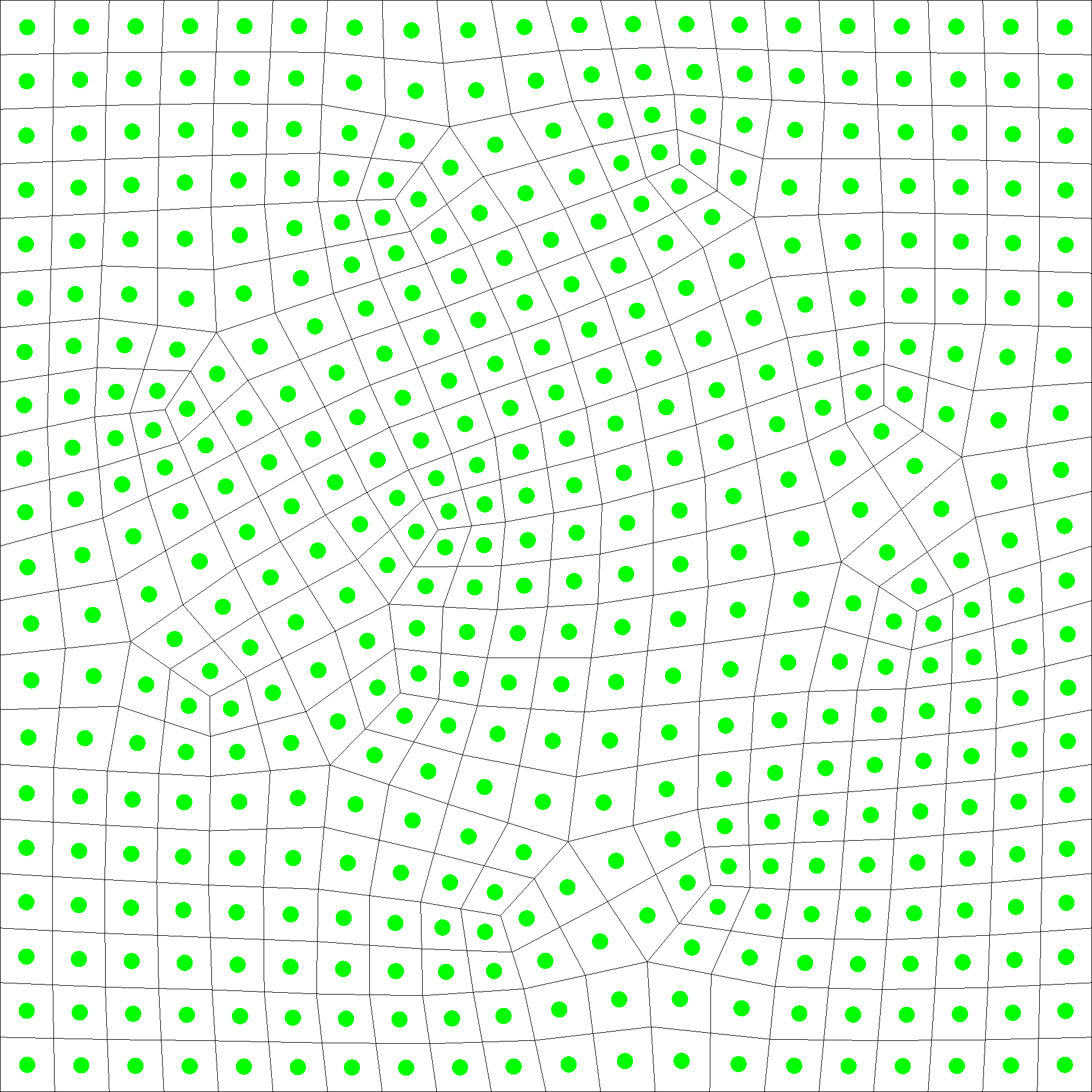
Figure 2: Initial particle arrangement for the patch test stability example. A random initial particle configuration is obtained by discretizing a square patch into 444 quadliteral area elements using a stochastic algorithm based on triangular Voronoi tesselation and recombination of the triangles into quadliterals. The particle coordinates are taken to be the quadliteral element centers and particle volumes are taken as the quadliteral area times a unit thickness.

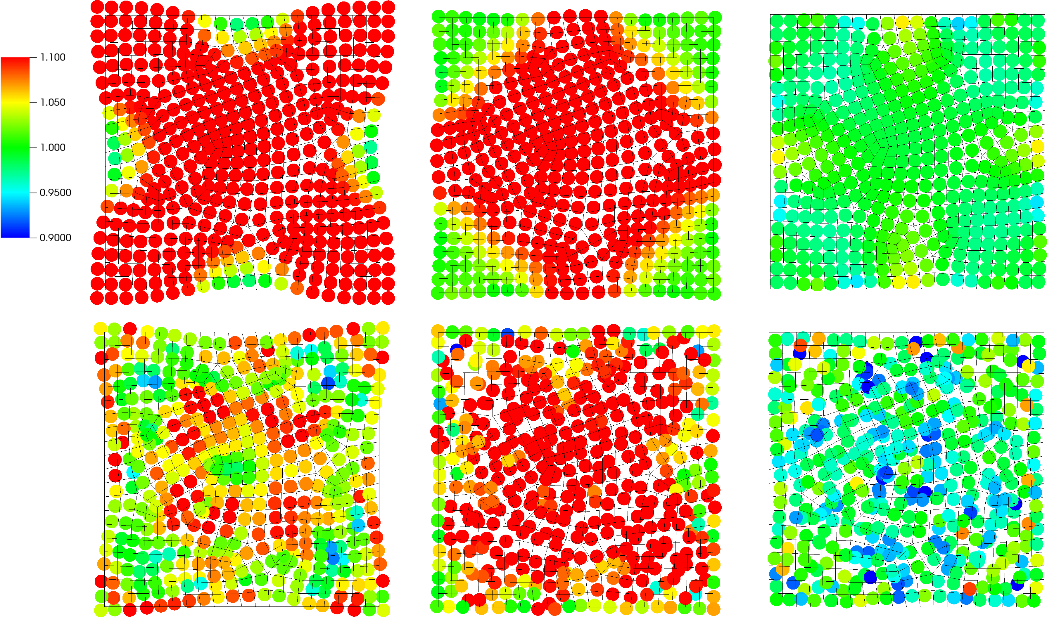
Figure 3: Simulation snapshots comparing unstabilized and stabilized trajectories. A 2d patch of an elastic material is perturbed by isotropic stretch of 10 % and integrated in time, resulting in a periodic contraction and expansion mode. The top row of images shows a stabilized solution during the first, third, and tenth contraction period. The bottom row shows corresponding snapshots from an unstabilized simulation. The mesh in the background serves as a guide to the eye.

5.3 Bending of a beam

This example considers a large deflection of a simply supported 2d beam with dimensions $8\,\mathrm{mm}\times 1\,\mathrm{mm}$, see Fig. 4. The material model of the beam is taken as linear elastic with Youngs modulus $E=100\,\mathrm{GPa}$ and $\nu=0.3$. A large boundary displacement of $u_{y}=8\,\mathrm{mm}$ is applied, and plain Total-Lagrangian SPH results (equivalent to Peridynamics with nodal integration) are qualitatively compared against a stabilized simulation code. Snapshots of the simulations corresponding to the same boundary displacements, are shown in Fig. 5. In the first snapshot at $u_{y}=4.8\,\mathrm{mm}$, no obvious difference between both simulations can be observed. For the second snapshot at $u_{y}=6.6\,\mathrm{mm}$, the unstabilized simulation shows a pattern where pairs of particles in the interior of the beam move together and do not follow the rotation of the beam’s neutral line. Clearly, the unstabilized system tries to minimize its elastic energy by assuming a configuration which is not in agreement with a linear displacement field. This leads to an obviously wrong particle configuration for the last snapshot at $u_{y}=8.0\,\mathrm{mm}$. In contrast, the stabilized system shows particle displacements which appear very reasonable and exhibit no instability.

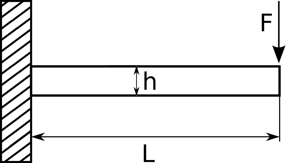
Figure 4: Sketch of the simply supported beam with dimensions $L=8\,\mathrm{mm}$ and $h=1\,\mathrm{mm}$.

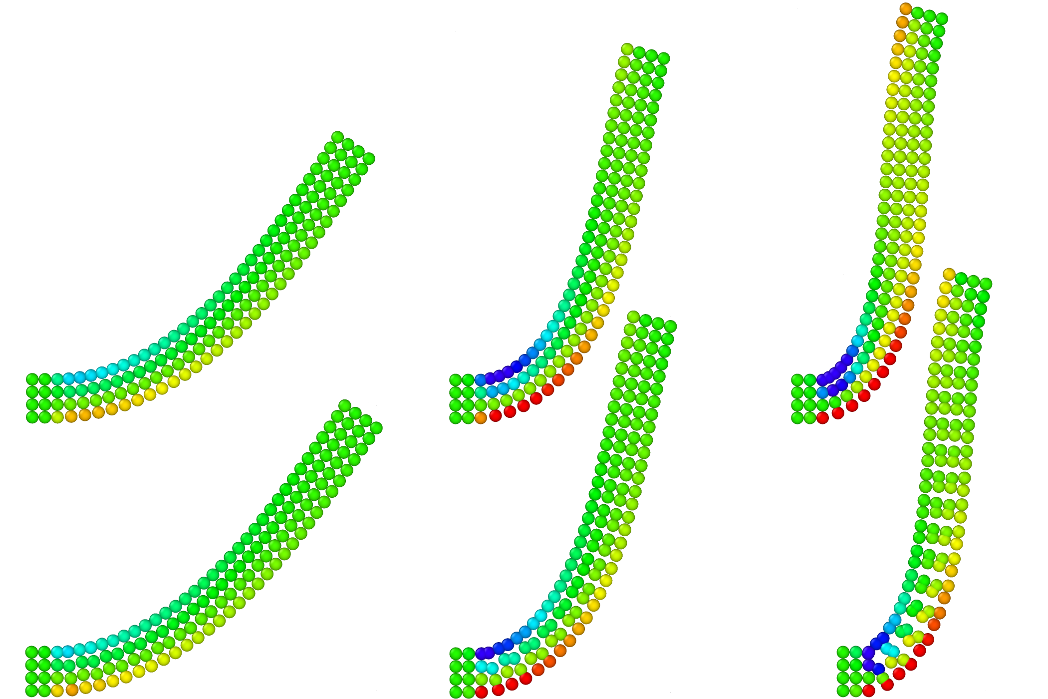
Figure 5: Comparison of stabilized (top) and unstabilized results for a large deflection simulation of the simply supported beam. The color coding represents the $xx$-component of the Second Piola-Kirchhoff stress tensor, with red signifying tension and blue compression.

We conclude this test case by noting that Total-Lagrangian SPH, or – equivalently – Peridynamics for classical material models based on the deformation gradient and with nodal integration, can become unstable for certain loading conditions even with perfectly uniform reference particle configurations. Hence, stabilization techniques, e.g. based on higher-order derivatives [27] are required to stabilize the solution.

6 Discussion

This work shows that Peridynamics – when used with classical material models based on the deformation gradient tensor and nodal integration as discretization technique – is equivalent to Total Lagrangian SPH with corrected gradients. This result allows to characterize this flavour of Peridynamics using the large body of studies published for SPH. SPH is a collocation method with nodal integration that suffers from two major problems: (i) the tensile instability, i.e., a numerical instability which results in particle clumping under conditions of negative pressure, and (ii) susceptibility to zero-energy modes which are caused by rank-deficiency due to nodal integration. Of these problems, the tensile instability is resolved by the Total-Lagrangian formulation [13, 19], and the rank-deficiency can be eliminated by using additional integration points [21]. Peridynamics with classical material models as presented here is a Total-Lagrangian method and therefore shows no tensile instability. However, if due to the use of nodal integration, it is still a rank-deficient method.

The rank-deficiency does usually not manifest itself until the reference configuration is updated. Such an update can be required as the Total-Lagrangian nature imposes restrictions on the magnitude of deformations that can be handled with the approximate deformation gradient. Alternatively, features of the material model, e.g. plasticity or failure, may require updates of the reference configuration. These updates result in zero-energy modes which need to be treated with dissipative mechanisms [27].

With the equivalence demonstrated in this work, Peridynamics applied to classical material models and in combination with nodal integration does not result in a new numerical method, but is instead a new derivation of an existing meshless method that is not free of problems. What are the implications of these findings for the other Peridynamic theories? The bond-based theory [7], which can be interpreted as an upscaling of the established meshless method Molecular Dynamics [28], does not require the calculation of a deformation gradient and thus does not suffer from the associated problems due to rank-deficiency. The state-based Peridynamic theory has also been formulated for some material models which are not based on the classical deformation gradient. If these unconventional material models, e.g., the linear Peridynamic solid [8], are discretized using nodal integration for computing dilatation and shear strain, rank deficiency problems are also likely to emerge.

Recently, work relating the reproducing Kernel Particle Method (RKPM) to state-based Peridynamics was published by Bessa et al [14]. In their work, the authors conclude that state-based Peridynamics is equivalent to RKPM if nodal integration, i.e., collocation, is used. These authors positively emphasize that the Peridynamic state-based approach is much faster compared to RKPM using more elaborate (cell based) integration techniques. These results are also understandable in light of this publication, because, it is known that RKPM with nodal integration is equivalent to Moving-Least-Squares SPH (MLSPH), which is known to be equivalent to SPH with corrected derivatives. For a comprehensive review on this equivalence, which also addresses the question as to how many really different meshless methods are known, see [29]. However, Bessa et al [14] disregard the unfortuitous implication of the equivalence of Peridynamics, SPH, and RKPM with nodal integration: we have learned from a number of SPH publications, that nodal integration causes problems, as it gives rise to zero-energy modes. Therefore the use of nodal integration for Peridynamics is a bad thing to do.

It is worthwhile to emphasize that the mathematical foundation of Peridynamics is clear and straightforward. Correct equations of motion emerge from this theory which conserve linear and angular momentum, and approximate linear fields accurately. All of these desirable features can only introduced into the SPH approximation by ad-hoc procedures. e.g. explicit symmetrization. Thus, if anything, the Peridynamic theory provides us with a better route to deriving meshless discretizations than the SPH method. If the simplest form of meshless discretization, namely nodal integration, is used, the advantages of Peridynamics over SPH vanish and the discrete expressions of both methods become equal. Stabilization schemes which address the rank-deficiency problem such as the scheme due to Vidal et al. [27] then need to be employed in order to keep the simulation stable. Future work should therefore address enhanced integration schemes for the Peridynamic theory.

References

- [1] S. A. Silling, Reformulation of elasticity theory for discontinuities and long-range forces, Journal of the Mechanics and Physics of Solids 48 (1) (2000) 175–209.
- [2] A. F. Bower, Applied Mechanics of Solids, CRC Press, 2011.
- [3] S. A. Silling, O. Weckner, E. Askari, F. Bobaru, Crack nucleation in a peridynamic solid, International Journal of Fracture 162 (1-2) (2010) 219–227.
- [4] Y. D. Ha, F. Bobaru, Studies of dynamic crack propagation and crack branching with peridynamics, International Journal of Fracture 162 (1-2) (2010) 229–244.
- [5] Y. D. Ha, F. Bobaru, Characteristics of dynamic brittle fracture captured with peridynamics, Engineering Fracture Mechanics 78 (6) (2011) 1156–1168.
- [6] A. Agwai, I. Guven, E. Madenci, Predicting crack propagation with peridynamics: a comparative study, International Journal of Fracture 171 (1) (2011) 65–78.
- [7] S. A. Silling, E. Askari, A meshfree method based on the peridynamic model of solid mechanics, Computers & Structures 83 (17–18) (2005) 1526–1535.
- [8] S. A. Silling, M. Epton, O. Weckner, J. Xu, E. Askari, Peridynamic states and constitutive modeling, Journal of Elasticity 88 (2) (2007) 151–184.
- [9] T. L. Warren, S. A. Silling, A. Askari, O. Weckner, M. A. Epton, J. Xu, A non-ordinary state-based peridynamic method to model solid material deformation and fracture, International Journal of Solids and Structures 46 (5) (2009) 1186–1195.
- [10] J. T. Foster, S. A. Silling, W. W. Chen, Viscoplasticity using peridynamics, Int J. Numer. Eng. 81 (10) (2010) 1242–1258.
- [11] S. A. Silling, R. B. Lehoucq, Convergence of peridynamics to classical elasticity theory, Journal of Elasticity 93 (1) (2008) 13–37.
- [12] J. W. Swegle, D. L. Hicks, S. W. Attaway, Smoothed particle hydrodynamics stability analysis, Journal of Computational Physics 116 (1) (1995) 123–134.
- [13] T. Belytschko, Y. Guo, W. Kam Liu, S. Ping Xiao, A unified stability analysis of meshless particle methods, International Journal for Numerical Methods in Engineering 48 (9) (2000) 1359–1400.
- [14] M. Bessa, J. Foster, T. Belytschko, W. Liu, A meshfree unification: reproducing kernel peridynamics, Computational Mechanics 53 (6) (2014) 1251–1264. doi:10.1007/s00466-013-0969-x.
- [15] V. P. Nguyen, T. Rabczuk, S. Bordas, M. Duflot, Meshless methods: a review and computer implementation aspects, Mathematics and computers in simulation 79 (3) (2008) 763–813.
- [16] T. Rabczuk, S. Bordas, G. Zi, On three-dimensional modelling of crack growth using partition of unity methods, Computers & structures 88 (23) (2010) 1391–1411.
- [17] L. B. Lucy, A numerical approach to the testing of the fission hypothesis, The Astronomical Journal 82 (1977) 1013–1024.
- [18] J. Bonet, S. Kulasegaram, Alternative total lagrangian formulations for corrected smooth particle hydrodynamics (CSPH) methods in large strain dynamic problems, Revue Europénne des Éléments 11 (7-8) (2002) 893–912.
- [19] T. Rabczuk, T. Belytschko, S. Xiao, Stable particle methods based on lagrangian kernels, Computer Methods in Applied Mechanics and Engineering 193 (12-14) (2004) 1035–1063.
- [20] R. Vignjevic, J. Reveles, J. Campbell, SPH in a total lagrangian formalism, Computer Modelling in Engineering and Sciences 146 (2) (3) (2006) 181–198.
- [21] P. Randles, L. Libersky, Smoothed Particle Hydrodynamics: Some recent improvements and applications, Computer Methods in Applied Mechanics and Engineering 139 (1) (1996) 375–408.
- [22] J. Bonet, T.-S. Lok, Variational and momentum preservation aspects of Smooth Particle Hydrodynamic formulations, Computer Methods in Applied Mechanics and Engineering 180 (1–2) (1999) 97–115.
- [23] R. Vignjevic, J. Campbell, L. Libersky, A treatment of zero-energy modes in the Smoothed Particle Hydrodynamics method, Computer Methods in Applied Mechanics and Engineering 184 (1) (2000) 67–85.
- [24] R. Gingold, J. Monaghan, Kernel estimates as a basis for general particle methods in hydrodynamics, Journal of Computational Physics 46 (3) (1982) 429–453.
-
[25]
M. Müller, R. Keiser, A. Nealen, M. Pauly, M. Gross, M. Alexa,
Point based animation of
elastic, plastic and melting objects, in: Proceedings of the 2004 ACM
SIGGRAPH/Eurographics Symposium on Computer Animation, SCA ’04, Eurographics
Association, Aire-la-Ville, Switzerland, Switzerland, 2004, pp. 141–151.
doi:10.1145/1028523.1028542.
URL http://dx.doi.org/10.1145/1028523.1028542 - [26] P. Lancaster, K. Salkauskas, Surfaces generated by moving least squares methods, Math. Comp. 37 (1981) 141 – 158.
- [27] Y. Vidal, J. Bonet, A. Huerta, Stabilized updated Lagrangian corrected SPH for explicit dynamic problems, International Journal for Numerical Methods in Engineering 69 (13) (2007) 2687–2710.
- [28] P. Seleson, M. L. Parks, M. Gunzburger, R. B. Lehoucq, Peridynamics as an upscaling of molecular dynamics, Multiscale Modeling & Simulation 8 (1) (2009) 204–227.
- [29] Y. Vidal, Mesh-free methods for dynamic problems – incompressibility and large strains, Ph.D. thesis, Universitat Politecnica de Catalunya, Barcelona, Spain (2004).