Post-Markovian quantum master equations from classical environment fluctuations

Abstract

In this paper we demonstrate that two commonly used phenomenological post-Markovian quantum master equations can be derived without using any perturbative approximation. A system coupled to an environment characterized by self-classical configurational fluctuations, the latter obeying a Markovian dynamics, defines the underlying physical model. Both Shabani-Lidar equation [A. Shabani and D. A. Lidar, Phys. Rev. A 71, 020101(R) (2005)] and its associated approximated integro-differential kernel master equation are obtained by tracing out two different bipartite Markovian Lindblad dynamics where the environment fluctuations are taken into account by an ancilla system. Furthermore, conditions under which the non-Markovian system dynamics can be unravelled in terms of an ensemble of measurement trajectories are found. In addition, a non-Markovian quantum jump approach is formulated. Contrary to recent analysis [L. Mazzola, E. M. Laine, H. P. Breuer, S. Maniscalco, and J. Piilo, Phys. Rev. A 81, 062120 (2010)], we also demonstrate that these master equations, even with exponential memory functions, may lead to non-Markovian effects such as an environment-to-system backflow of information if the Hamiltonian system does not commutate with the dissipative dynamics.

I Introduction

Contrary to Markovian Lindblad dynamics alicki ; breuerbook , the description of non-Markovian open quantum systems relies on density matrix evolutions defined by integro-differential equations haake . In these dynamics, the dependence of the system state on its previous history is weighted by a memory kernel function, which in turn may itself depend on each dissipative channel. Different theoretical approaches and physical situations had been analyzed by many authors in order to establish and characterize these equations stenholm ; classBu ; giraldi ; VacCol ; tanos ; wilkie ; salo ; cresser ; Lidar ; ManisPetru ; unMedio ; piilo ; grano ; LindbladRate ; vacchini ; SemiMarkov ; Kosa ; NoMeasure . The unravelling of the non-Markovian dynamics in terms of measurement trajectories has also been extensively studied diosi ; maniscalco ; petruccione ; barchielli ; BuJumpSMS ; OneChannel ; Embedding .

On the basis of a phenomenological measurement theory Shabani and Lidar introduced a non-Markovian dynamics Lidar , called post-Markovian equation, where a single kernel weights the memory effects. In the “stationary case” it is

$$\frac{d}{dt}\rho_{t}^{s}=\mathcal{C}_{s}\int_{0}^{t}dt^{\prime}k(t-t^{\prime})\exp[(t-t^{\prime})\mathcal{C}_{s}]\rho_{t^{\prime}}^{s},$$ (1)

where $\rho_{t}^{s}$ is the system density matrix and $\mathcal{C}_{s}$ is an arbitrary (diagonalized) Lindblad superoperator,

$$\mathcal{C}_{s}[\rho]=\frac{1}{2}\sum_{\alpha}\gamma_{\alpha}([V_{\alpha},\rho V_{\alpha}^{{\dagger}}]+[V_{\alpha}\rho,V_{\alpha}^{{\dagger}}]),\ \ \ \ \ \{\gamma_{\alpha}\}\geq 0.$$ (2)

The rates $\{\gamma_{\alpha}\}$ “measure” the weight of each dissipative Lindblad channel defined by the system operators $\{V_{\alpha}\}.$ As mentioned in Lidar , under the condition $||\mathcal{C}_{s}||\ll 1/t,$ the previous equation can be approximated as

$$\frac{d}{dt}\rho_{t}^{s}=\mathcal{C}_{s}\int_{0}^{t}dt^{\prime}k(t-t^{\prime})\rho_{t^{\prime}}^{s},$$ (3)

which shows the close relationship that exists between both types of non-Markovian evolutions, Eqs. (1) and (3).

Different analysis of both non-Markovian master equations can be found in literature ManisPetru ; unMedio ; piilo ; grano . In Ref. ManisPetru , by comparing the solutions of both equations for a qubit system, conditions on the limit of applicability of each dynamics were established. In Ref. unMedio , the completely positive condition alicki ; breuerbook of the solution maps was studied by assuming an exponential kernel. In that case, Eq. (1) always results in a completely positive solution map while Eq. (3) does not fulfill this condition, in general stenholm ; classBu . In Ref. piilo it was found that neither Eq. (1) nor Eq. (3) are able to induce “genuine” non-Markovian effects such as an environment-to-system backflow of information NoMeasure . A stringent constraint on the usefulness of these equations is established by this result. In addition, the hazards of using non-Markovian evolutions like Eq. (1) in systems containing a partially unitary dynamics were analyzed in Ref. grano .

In spite of the previous analysis ManisPetru ; unMedio ; piilo ; grano , consistently with its original formulation Lidar , the non-Markovian evolutions (1) and (3) rely on phenomenological ingredients such as the memory kernel $k(t).$ In fact, microscopic dynamics that lead to a given kernel are generally unknown. On the other hand, assuming that a continuous-in-time measurement process is performed over the system, it is not known which kind of stochastic trajectories plenio ; carmichaelbook ; carmichael ; barchiellibook ; bartano  may describe the conditional system dynamics diosi ; maniscalco ; petruccione ; barchielli ; BuJumpSMS ; OneChannel ; Embedding . The main goal of this paper is to answer these issues. In addition, we criticize and generalize some previous results ManisPetru ; unMedio ; piilo ; grano  about these non-Markovian dynamics.

Over the basis of single molecule spectroscopy arrangements SMS , in the present study we consider a system coupled to an environment characterized by (Markovian) classical self-fluctuations, which in turn modify or modulate the system dissipative dynamics. This situation can be described with a bipartite Lindblad evolution LindbladRate , where an auxiliary ancilla system takes into account the environment fluctuations SMSBudini . Under these assumptions, without introducing any perturbative approximation, by using projector techniques we demonstrate that Eqs. (1) and (3) describe the system dynamics for two alternative kinds of system-environment couplings. On the other hand, generalizing the results of Ref. OneChannel , we show that, under some particular conditions, a non-Markovian quantum jump approach can be consistently formulated for both non-Markovian master equations. In fact, under specific symmetries conditions, non-Markovian evolutions obtained from a partial trace over a bipartite Markovian dynamics can be unravelled in terms of a set of measurement trajectories whose dynamics can be written in the (single) system Hilbert space OneChannel .

We remark that in the present study the Lindblad superoperator (2) that defines both master equations (1) and (3) is not a “collisional” one Embedding , that is,

$$\mathcal{C}_{s}\neq\sum_{\alpha}V_{\alpha}\rho V_{\alpha}^{{\dagger}}-\mathrm{I}_{s},\ \ \ \ \ \ \ \ \ \ \sum_{\alpha}V_{\alpha}^{{\dagger}}V_{\alpha}=\mathrm{I}_{s},$$ (4)

where $\mathrm{I}_{s}$ is the identity matrix. When $\mathcal{C}_{s}=\sum_{\alpha}V_{\alpha}\rho V_{\alpha}^{{\dagger}}-\mathrm{I}_{s},$ the non-Markovian dynamics (3) can be unravelled in terms of a set of trajectories where the collisional superoperator $\mathcal{E}_{s}[\rho]=\sum_{\alpha}V_{\alpha}\rho V_{\alpha}^{{\dagger}}$ is applied at random times over the system state Embedding . As a consequence of the assumption (4), the results of Ref. Embedding do not apply in the present context.

The paper is structured as follows. In Sec. II, we present the basic bipartite Markovian model that describes the system-environment coupling. Both evolutions (1) and (3) are obtained by tracing out the configurational bath-fluctuations. In Sec. III, for each equation we develop a non-Markovian quantum jump approach that allows to unravel the dynamics in terms of a set of measurement trajectories. Conditions under which these results can be formulated are found in the Appendix. In Sec. IV we study an example that exhibits the main features of the present approach. Furthermore, the model shows that, even with an exponential memory kernel function, the analyzed post-Markovian quantum master equations may lead to the development of genuine non-Markovian effects. In Sec. V we provide the Conclusions.

II Classical environment fluctuations

We consider a system $S$ interacting with an environment that develops classical self-fluctuations between a set of “configurational bath-states” vanKampen . Each state corresponds to different Hilbert subspaces of the reservoir which are able to induce by themselves a different Markovian system dynamics. Hence, the transitions between them modulate the system evolution SMS ; SMSBudini .

The transitions between the reservoir-states are defined by a classical Pauli master equation vanKampen

$$\frac{d}{dt}p_{t}^{i}=\sum_{j}(\phi_{ij}p_{t}^{j}-\phi_{ji}p_{t}^{i}),$$ (5)

where $p_{t}^{i}$ is the probability that at time $t$ the environment is in the $i-$state $(i=0,1,\cdots i_{\max})$ while $\phi_{ij}$ are the transition rates $(\phi_{ij}\geq 0,$ $\phi_{ii}=0).$ The system density matrix $\rho_{t}^{s}$ is written as

$$\rho_{t}^{s}=\sum_{i}\rho_{t}^{i},$$ (6)

where each auxiliary state $\rho_{t}^{i}$ corresponds to the system state “given” that the environment is in the $i-$state LindbladRate . The weight of each bath-state is encoded as $p_{t}^{i}=\mathrm{Tr}_{s}\left[\rho_{t}^{i}\right].$ The initial conditions read $\{\rho_{0}^{i}=p_{0}^{i}\rho_{0}^{s}\}.$ The system dynamics is completely defined after introducing the time evolution of the states $\rho_{t}^{i}.$ We consider models where the bath-states modulate (modify) the system dissipative dynamics. In correspondence with Eqs. (1) and (3) two different cases are considered.

First case

In the first case, the evolution of the auxiliary states is given by the “Lindblad rate equation” LindbladRate

$$\frac{d}{dt}\rho_{t}^{i}=\mathcal{L}_{s}\rho_{t}^{i}+(1-\delta_{i0})\mathcal{C}_{s}\rho_{t}^{i}+\sum_{j}(\phi_{ij}\rho_{t}^{j}-\phi_{ji}\rho_{t}^{i}),$$ (7)

where $\delta_{ij}$ is the Kronecker delta function. The superoperator $\mathcal{L}_{s}$ defines the system unitary evolution, but may also include arbitrary Lindblad contributions. The action of $\mathcal{L}_{s}$ is independent of the environment state. On the other hand, the superoperator $\mathcal{C}_{s}$ is given by Eq. (2). Its action is modulated by the environment states. In fact, in Eq. (7), its influence is inhibited when the bath is in the state $i=0.$ In any other case $(i\neq 0),$ the system dynamics also includes the contribution $\mathcal{C}_{s}.$ The classical transitions between these regimes is introduced by the last term in Eq. (7), which in turn, from $p_{t}^{i}=\mathrm{Tr}_{s}\left[\rho_{t}^{i}\right],$ leads to the classical master equation (5).

Second case

The second dynamics is complementary to the previous one. The auxiliary states evolution is

$$\frac{d}{dt}\rho_{t}^{i}=\mathcal{L}_{s}\rho_{t}^{i}+\delta_{i0}\mathcal{C}_{s}\rho_{t}^{i}+\sum_{j}(\phi_{ij}\rho_{t}^{j}-\phi_{ji}\rho_{t}^{i}).$$ (8)

Therefore, here $\mathcal{C}_{s}$ is able to modify the system dynamics only when the environment is in the state $i=0.$ In any other case $(i\neq 0),$ it is inhibited. Notice that this “complementary bath action” is the unique difference with Eq. (7).

II.1 Bipartite representation

The system state (6) and the evolution defined by Eqs. (7) and (8) completely define the (non-Markovian) system dynamics. Nevertheless, their analysis is simplified if those dynamics are embedded in a bipartite Markovian dynamics LindbladRate , where an extra ancilla (auxiliary) system $(A)$ takes into account the environment fluctuations. The joint system-ancilla density matrix is denoted as $\rho_{t}^{sa}.$ From this object, the system state follows from a partial trace,

$$\rho_{t}^{s}=\mathrm{Tr}_{a}\left[\rho_{t}^{sa}\right]=\sum_{i}\left\langle a_{i}\right|\rho_{t}^{sa}\left|a_{i}\right\rangle,$$ (9)

where $\{\left|a_{i}\right\rangle\},$ $i=0,1\cdots(\dim\mathcal{H}_{a}-1)=i_{\max},$ is a complete normalized basis in the ancilla Hilbert space $\mathcal{H}_{a}.$ Each state $\left|a_{i}\right\rangle$ corresponds to each configurational bath-state. Hence, the auxiliary system states [Eq. (6)] read

$$\rho_{t}^{i}=\left\langle a_{i}\right|\rho_{t}^{sa}\left|a_{i}\right\rangle,$$ (10)

while the ancilla populations

$$p_{t}^{i}=\mathrm{Tr}_{s}\left[\rho_{t}^{i}\right]=\left\langle a_{i}\right|\mathrm{Tr}_{s}\left[\rho_{t}^{sa}\right]\left|a_{i}\right\rangle,$$ (11)

define the probability of each configurational bath-state. From now on we denote indistinctly the bath-states by their ancilla representation.

The time evolution of $\rho_{t}^{sa}$ is given by a Markovian equation that recovers the previous Lindblad rate equations. It is written as

$$\frac{d}{dt}\rho_{t}^{sa}=\mathcal{L}[\rho_{t}^{sa}]=(\mathcal{L}_{s}+\mathcal{L}_{a}+\mathcal{C}_{sa})\rho_{t}^{sa}.$$ (12)

The superoperator $\mathcal{L}_{s}$ is the same as before and only acts on the system Hilbert space. The contribution $\mathcal{L}_{a}$ gives the ancilla dynamics. It introduces the configurational bath-transitions. In correspondence with the classical evolution (5), it reads

$$\mathcal{L}_{a}[\rho]=\frac{1}{2}\sum_{i,j}\phi_{ij}([A_{ij},\rho A_{ij}^{{\dagger}}]+[A_{ij}\rho,A_{ij}^{{\dagger}}]).$$ (13)

The operators are $A_{ij}=\mathrm{I}_{s}\otimes\left|a_{i}\right\rangle\left\langle a_{j}\right|.$

The contribution $\mathcal{C}_{sa}$ is defined in different ways for each case. In the first case, it must be taken as

$$\mathcal{C}_{sa}[\rho]=\frac{1}{2}\sum\nolimits_{i,\alpha}^{{}^{\prime}}\gamma_{\alpha}([T_{\alpha i},\rho T_{\alpha i}^{{\dagger}}]+[T_{\alpha i}\rho,T_{\alpha i}^{{\dagger}}]),$$ (14)

where the Lindblad bipartite operators are

$$T_{\alpha i}=V_{\alpha}\otimes\left|a_{i}\right\rangle\left\langle a_{i}\right|.$$ (15)

Both the rates $\{\gamma_{\alpha}\}$ and system operators $\{V_{\alpha}\}$ are the same as in Eq. (2). With $\sum\nolimits_{i}^{{}^{\prime}}$ we denote a sum that runs over the states $\left|a_{i}\right\rangle,$ $i=1,\cdots(\dim\mathcal{H}_{a}-1),$ excluding the state $\left|a_{\mathrm{0}}\right\rangle.$ By using the definition of the auxiliary states, Eq. (10), from the bipartite dynamics (12), jointly with the definitions (13) and (14), it is simple to recover the Lindblad rate equation corresponding to the first case, Eq. (7). On the other hand, the second case, Eq. (8), follows by defining the contribution $\mathcal{C}_{sa}$ as

$$\mathcal{C}_{sa}[\rho]=\frac{1}{2}\sum_{\alpha}\gamma_{\alpha}([T_{\alpha 0},\rho T_{\alpha 0}^{{\dagger}}]+[T_{\alpha 0}\rho,T_{\alpha 0}^{{\dagger}}]),$$ (16)

where the operators $\{T_{\alpha 0}\}$ are

$$T_{\alpha 0}=V_{\alpha}\otimes\left|a_{\mathrm{0}}\right\rangle\left\langle a_{\mathrm{0}}\right|.$$ (17)

Notice that in this case [Eq. (16)] an addition over the ancilla states [Eq. (14)] is not necessary.

II.2 Non-Markovian system dynamics

By using projector techniques breuerbook ; haake , from the bipartite reformulation [Eq. (12)] it is possible to obtain the system density matrix evolution. Let introduce the projectors $\mathcal{P}$ and $\mathcal{Q}$,

$$\mathcal{P}\rho_{t}^{sa}=\mathrm{Tr}_{a}\left[\rho_{t}^{sa}\right]\otimes\left|a_{\mathrm{0}}\right\rangle\left\langle a_{\mathrm{0}}\right|,\ \ \ \ \ \ \ \ \mathcal{P}+\mathcal{Q}=\mathrm{I}_{sa},$$ (18)

where $\mathrm{I}_{sa}$ is the identity matrix in the bipartite system-ancilla Hilbert space. As usual breuerbook ; haake , the bipartite evolution (12) can be projected in relevant and irrelevant contributions

$$\frac{d}{dt}\mathcal{P}\rho_{t}^{sa} = \mathcal{PL(P}+\mathcal{Q})\rho_{t}^{sa},$$ (19)

$$\frac{d}{dt}\mathcal{Q}\rho_{t}^{sa} = \mathcal{QL(P}+\mathcal{Q})\rho_{t}^{sa}.$$ (20)

On the other hand, as an initial condition we consider a separable bipartite state

$$\rho_{0}^{sa}=\rho_{0}^{s}\otimes\Pi_{\mathrm{0}}=\rho_{0}^{s}\otimes\left|a_{\mathrm{0}}\right\rangle\left\langle a_{\mathrm{0}}\right|,$$ (21)

where $\rho_{0}^{s}$ is an arbitrary system state. Hence, the ancilla begins in the pure state $\Pi_{\mathrm{0}}=\left|a_{\mathrm{0}}\right\rangle\left\langle a_{\mathrm{0}}\right|,$ which in turn implies that the initial bath-state is $i=0$ $[p_{0}^{i}=\delta_{i0}$ in Eq. (5)].

Given the initial bipartite state (21), it follows that $\mathcal{Q}\rho_{0}^{sa}=0.$ Therefore, Eq. (20) can be integrated as $\mathcal{Q}\rho_{t}^{sa}=\int_{0}^{t}dt^{\prime}\exp[\mathcal{QL}(t-t^{\prime})]\mathcal{QLP}\rho_{t^{\prime}}^{sa},$ which in turn, after replacing in Eq. (19), leads to the convoluted evolution haake

$$\frac{d}{dt}\mathcal{P}\rho_{t}^{sa}=\mathcal{PLP}\rho_{t}^{sa}+\mathcal{PL}\int_{0}^{t}dt^{\prime}\exp[\mathcal{QL}(t-t^{\prime})]\mathcal{QLP}\rho_{t^{\prime}}^{sa}.$$ (22)

An explicit system density matrix evolution can be obtained from this general expression. Its structure depends on each case.

First case

The bipartite superoperator $\mathcal{L}$ is defined by Eq. (12). Taking into account Eq. (14) it can be written as

$$\mathcal{L}[\bullet] = (\mathcal{L}_{s}+\mathcal{L}_{a})[\bullet]-\frac{1}{2}\sum\nolimits_{\alpha i}^{{}^{\prime}}\gamma_{\alpha}\{V_{\alpha}^{{\dagger}}V_{\alpha}\otimes\Pi_{i},\bullet\}_{+}$$ (23)

$$+\sum\nolimits_{\alpha i}^{{}^{\prime}}\gamma_{\alpha}V_{\alpha}\left\langle a_{i}\right|\bullet\left|a_{i}\right\rangle V_{\alpha}^{{\dagger}}\otimes\Pi_{i},$$

where $\Pi_{i}\equiv\left|a_{i}\right\rangle\left\langle a_{i}\right|,$ and $\{.,.\}_{+}$ denotes an anticommutator operation. With this expression it is possible to evaluate all contributions in Eq. (22). We get

$$\mathcal{PL}[\bullet]=\{\mathcal{L}_{s}(\mathrm{Tr}_{a}\left[\bullet\right])+\mathcal{C}_{s}[\sum\nolimits_{i}^{{}^{\prime}}\left\langle a_{i}\right|\bullet\left|a_{i}\right\rangle]\}\otimes\Pi_{\mathrm{0}},$$ (24)

where $\mathcal{C}_{s}$ is given by Eq. (2). Hence, it follows the result $\mathcal{PLP}\rho_{t}^{sa}=\mathcal{L}_{s}\rho_{t}^{s}\otimes\Pi_{\mathrm{0}}.$ Furthermore, $\mathcal{QLP}\rho_{t^{\prime}}^{sa}=\rho_{t^{\prime}}^{s}\otimes\mathcal{L}_{a}[\Pi_{\mathrm{0}}].$ Using the classicality of the ancilla dynamics, Eq. (13), $\left\langle a_{i}\right|\mathcal{L}_{a}[\rho_{t}]\left|a_{i}\right\rangle=\left\langle a_{i}\right|\mathcal{L}_{a}[\sum_{j}\left\langle a_{j}\right|\rho_{t}\left|a_{j}\right\rangle\otimes\Pi_{j}]\left|a_{i}\right\rangle$ (populations are only coupled to populations), it is also possible to obtain $(\mathcal{QL})^{n}(\rho_{t^{\prime}}^{s}\otimes\mathcal{L}_{a}[\Pi_{\mathrm{0}}])=(\mathcal{L}_{s}+\mathcal{C}_{s}+\mathcal{L}_{a})^{n}(\rho_{t^{\prime}}^{s}\otimes\mathcal{L}_{a}[\Pi_{\mathrm{0}}]),$ with $n=1.$ The validity of this expression for $n=2,3,\cdots$ can be demonstrated by using the mathematical principle of induction. Hence, we get

$$\exp[\mathcal{QL}t]\mathcal{QLP}\rho_{t^{\prime}}^{sa}=\exp[(\mathcal{L}_{s}+\mathcal{C}_{s}+\mathcal{L}_{a})t](\rho_{t^{\prime}}^{s}\otimes\mathcal{L}_{a}[\Pi_{\mathrm{0}}]).$$ (25)

After introducing the previous results in Eq. (22) we obtain the non-Markovian master equation

$$\frac{d}{dt}\rho_{t}^{s}\!=\!\mathcal{L}_{s}\rho_{t}^{s}+\mathcal{C}_{s}\int_{0}^{t}dt^{\prime}k_{\mathrm{I}}(t-t^{\prime})\{\exp[(t-t^{\prime})(\mathcal{L}_{s}+\mathcal{C}_{s})]\rho_{t^{\prime}}^{s}\},$$ (26)

where the kernel function is defined in terms of the ancilla dynamics

$$k_{\mathrm{I}}(t) = \sum\nolimits_{i}^{{}^{\prime}}\left\langle a_{i}\right|\exp(t\mathcal{L}_{a})\mathcal{L}_{a}[\Pi_{\mathrm{0}}]\left|a_{i}\right\rangle,$$ (27a)

$$= \frac{d}{dt}\sum\nolimits_{i}^{{}^{\prime}}\left\langle a_{i}\right|\exp(t\mathcal{L}_{a})[\Pi_{\mathrm{0}}]\left|a_{i}\right\rangle.$$ (27b)

The trace preservation condition $$\sum_{i}\left\langle a_{i}\right|\mathcal{L}_{a}(\bullet)\left|a_{i}\right\rangle=0 (d/dt)\sum\nolimits_{i}p_{t}^{i}=0. \sum_{i}\left\langle a_{i}\right|\mathcal{L}_{a}(\bullet)\left|a_{i}\right\rangle=\left\langle a_{\mathrm{0}}\right|\mathcal{L}_{a}(\bullet)\left|a_{\mathrm{0}}\right\rangle+\sum_{i}^{\prime}\left\langle a_{i}\right|\mathcal{L}_{a}(\bullet)\left|a_{i}\right\rangle,$$ is consistent with Therefore, which leads to the equivalent expression

$$k_{\mathrm{I}}(t)=-\frac{d}{dt}\left\langle a_{\mathrm{0}}\right|\exp(t\mathcal{L}_{a})[\Pi_{\mathrm{0}}]\left|a_{\mathrm{0}}\right\rangle=-\frac{d}{dt}p_{t}^{0}.$$ (28)

Eq. (26) is one of the main results of this section. It provides a natural extension of Shabani-Lidar proposal. In fact, when the condition $[\mathcal{L}_{s},\mathcal{C}_{s}]=0$ is satisfied, in an “interaction representation” with respect to $\mathcal{L}_{s}$ it follows Eq. (1) with $k(t)\rightarrow k_{\mathrm{I}}(t).$ By construction (partial trace over a Lindblad dynamics) Eq. (26) is a completely positive evolution, generalizing in this way the results of Ref. unMedio . Notice that after defining the “system-reservoir” dynamics [Eq. (7)], we have not introduced any extra approximation in the derivation of this result. On the other hand, in the present approach the kernel function is completely determined by the dynamics of the classical environment fluctuations. In fact, given the initial condition Eq. (21), in Eq. (28) $p_{t}^{0}$ corresponds to the survival probability of the $i=0$ bath-state $[p_{0}^{i}=\delta_{i0}]$ that follows from Eq. (5). Notice that any kernel $k_{\mathrm{I}}(t)$ arising from this classical structure guarantees the completely positive condition of the solution map, $\rho_{0}^{s}\rightarrow\rho_{t}^{s}.$ If the bath transitions rates depend explicitly on time, $\{\phi_{ij}\}\rightarrow\{\phi_{ij}(t)\},$ the kernel becomes non-stationary, $k_{\mathrm{I}}(t)\rightarrow k_{\mathrm{I}}(\tau,t)$ Lidar . The corresponding master equation can be worked out in a similar way.

Second case

In the second case, taking into account the superoperator (16), the bipartite superoperator $\mathcal{L}$ [Eq. (12)] reads

$$\mathcal{L}[\bullet] = (\mathcal{L}_{s}+\mathcal{L}_{a})[\bullet]-\frac{1}{2}\sum_{\alpha}\gamma_{\alpha}\{V_{\alpha}^{{\dagger}}V_{\alpha}\otimes\Pi_{\mathrm{0}},\bullet\}_{+}$$ (29)

$$+\sum_{\alpha}\gamma_{\alpha}V_{\alpha}\left\langle a_{\mathrm{0}}\right|\bullet\left|a_{\mathrm{0}}\right\rangle V_{\alpha}^{{\dagger}}\otimes\Pi_{\mathrm{0}}.$$

From here, we obtain

$$\mathcal{PL}[\bullet]=\{\mathcal{L}_{s}(\mathrm{Tr}_{a}\left[\bullet\right])+\mathcal{C}_{s}[\left\langle a_{\mathrm{0}}\right|\bullet\left|a_{\mathrm{0}}\right\rangle]\}\otimes\Pi_{\mathrm{0}}.$$ (30)

Hence, it follows $\mathcal{PLP}\rho_{t}^{sa}=(\mathcal{L}_{s}+\mathcal{C}_{s})\rho_{t}^{s}\otimes\Pi_{\mathrm{0}},$ and $\mathcal{QLP}\rho_{t^{\prime}}^{sa}=\rho_{t^{\prime}}^{s}\otimes\mathcal{L}_{a}[\Pi_{\mathrm{0}}].$ As in the previous case, using the classicality of $\mathcal{L}_{a}$ it is also possible to obtain $\mathcal{QL}(\rho_{t^{\prime}}^{s}\otimes\mathcal{L}_{a}[\Pi_{\mathrm{0}}])=(\mathcal{L}_{s}+\mathcal{L}_{a})(\rho_{t^{\prime}}^{s}\otimes\mathcal{L}_{a}[\Pi_{\mathrm{0}}]),$ which by induction leads to

$$\exp[\mathcal{QL}t]\mathcal{QLP}\rho_{t^{\prime}}^{sa}=\exp[(\mathcal{L}_{s}+\mathcal{L}_{a})t](\rho_{t^{\prime}}^{s}\otimes\mathcal{L}_{a}[\Pi_{\mathrm{0}}]).$$ (31)

By introducing these results in Eq. (22) we get

$$\frac{d}{dt}\rho_{t}^{s}=(\mathcal{L}_{s}+\mathcal{C}_{s})\rho_{t}^{s}-\mathcal{C}_{s}\int_{0}^{t}dt^{\prime}k_{\mathrm{I}}(t-t^{\prime})\{\exp[(t-t^{\prime})\mathcal{L}_{s}]\rho_{t^{\prime}}^{s}\},$$

where $k_{\mathrm{I}}(t)$ is given by Eq. (28). This master equation can trivially be rewritten as

$$\frac{d}{dt}\rho_{t}^{s}=\mathcal{L}_{s}\rho_{t}^{s}+\mathcal{C}_{s}\int_{0}^{t}dt^{\prime}k_{\mathrm{II}}(t-t^{\prime})\{\exp[(t-t^{\prime})\mathcal{L}_{s}]\rho_{t^{\prime}}^{s}\}.$$ (32)

where the kernel function is $k_{\mathrm{II}}(t)=\delta(t)-k_{\mathrm{I}}(t).$ Hence,

$$k_{\mathrm{II}}(t) = \delta(t)+\frac{d}{dt}\left\langle a_{\mathrm{0}}\right|\exp(t\mathcal{L}_{a})[\Pi_{\mathrm{0}}]\left|a_{\mathrm{0}}\right\rangle,$$ (33a)

$$= \delta(t)+\frac{d}{dt}p_{t}^{0}.$$ (33b)

If $$[\mathcal{L}_{s},\mathcal{C}_{s}]=0, \mathcal{L}_{s}, k(t)\rightarrow k_{\mathrm{II}}(t).$$ in an interaction representation with respect to from Eq. (32) it follows Eq. (3) with Therefore, that equation is obtained, without introducing any approximation, from the alternative system-environment coupling defined by Eq. (8). This is the second main result of this section.

Contrary to the previous case [Eq. (28)], in this one the kernel includes a delta term, which in turn leads to a local in time contribution in the evolution (32). The presence of this term can be explained directly from Eq. (8). In fact, in the limit where the bath does not fluctuate, $\phi_{ij}\rightarrow 0,$ taking into account the initial condition (21), a Markovian Lindblad dynamics defined by $(\mathcal{L}_{s}+\mathcal{C}_{s})$ is recovered.

When the condition (4) is not satisfied, Eq. (32) can also be derived from a different underlying dynamics that gives an alternative expression for the memory kernel Embedding . As the present approach relies on condition (4), it provides an alternative basis for the derivation of Eq. (32), which in consequence can be applied in a larger range of dissipative dynamics.

II.3 Exponential kernels

Different analysis of Eqs. (1) and (3) were performed after assuming an exponential kernel ManisPetru ; unMedio ; piilo . In the present approach, this particular case arises when the environment has only two different configurational states, that is, the ancilla Hilbert space is defined by only two states, $\left|a_{\mathrm{0}}\right\rangle$ and $\left|a_{1}\right\rangle.$ The classical master equation (5) becomes

$$\frac{d}{dt}p_{t}^{0}=-\phi p_{t}^{0}+\varphi p_{t}^{1},\ \ \ \ \ \ \ \ \ \ \ \frac{d}{dt}p_{t}^{1}=-\varphi p_{t}^{1}+\phi p_{t}^{0}.$$ (34)

Here, the bath transition rates are denoted by $\phi$ and $\varphi.$ For normalized initial conditions $p_{0}^{0}+p_{0}^{1}=1,$ with $p_{0}^{0}=1,$ and $p_{0}^{1}=0$ [Eq. (21)] the solutions are

$$p_{t}^{0} = \frac{\varphi}{\phi+\varphi}+\exp[-t(\phi+\varphi)]\frac{\phi}{\phi+\varphi},$$ (35a)

$$p_{t}^{1} = \frac{\phi}{\phi+\varphi}-\exp[-t(\phi+\varphi)]\frac{\phi}{\phi+\varphi}.$$ (35b)

Thus, the kernel (28) reads

$$k_{\mathrm{I}}(t)=\phi\exp[-t(\phi+\varphi)],$$ (36)

while in the second case, Eq. (33), it follows

$$k_{\mathrm{II}}(t)=\delta(t)-\phi\exp[-t(\phi+\varphi)].$$ (37)

In this way, our formalism associates a very simple environment structure to these kinds of kernels. Notice that in the second case, Eq. (37), the exponential contribution is accompanied by a local in time contribution. In fact, as well known stenholm ; classBu , Eq. (3) with a single exponential kernel does not lead in general to a completely positive dynamics ManisPetru ; unMedio . Hence, the delta contribution avoids the lack of the completely positive condition of the solution map. On the other hand, both kernels, as well as the underlying physical dynamics, are well defined for any value of the parameters. In particular when $\varphi=0.$

II.4 Extension to non-interacting bipartite systems

In Ref. grano the authors analyzed a generalization of Eq. (1) for two systems, where one of them obeys a unitary evolution. That situation can be easily described in the present frame. Apart from the system $S,$ we consider another system $S^{\prime}.$ The single evolution of $S^{\prime}$ is local in time (Markovian) and defined by a superoperator $\mathcal{L}_{s^{\prime}}.$ Then, we ask about the evolution of the bipartite density matrix $\rho_{t}^{ss^{\prime}}$ associated to both systems. This question can be straightforwardly answered from Eq. (26) by taking as system the bipartite extension $S\otimes S^{\prime}.$ Therefore, under the replacements $\rho_{t}^{s}\rightarrow\rho_{t}^{ss^{\prime}}$ and $\mathcal{L}_{s}\rightarrow(\mathcal{L}_{s}+\mathcal{L}_{s^{\prime}}),$ $\mathcal{C}_{s}\rightarrow\mathcal{C}_{s}\otimes\mathrm{I}_{s^{\prime}},$ where $\mathrm{I}_{s^{\prime}}$ is the identity matrix, it follows

$$\frac{d}{dt}\rho_{t}^{ss^{\prime}}=(\mathcal{L}_{s}+\mathcal{L}_{s^{\prime}})\rho_{t}^{ss^{\prime}}+\mathcal{C}_{s}\int_{0}^{t}dt^{\prime}k_{\mathrm{I}}(t^{\prime})e^{t^{\prime}(\mathcal{L}_{s}+\mathcal{L}_{s^{\prime}}+\mathcal{C}_{s})}\rho_{t-t^{\prime}}^{ss^{\prime}}.$$ (38)

Assuming a separable initial bipartite state, $\rho_{0}^{ss^{\prime}}=\rho_{0}^{s}\otimes$ $\rho_{0}^{s^{\prime}},$ the solution of Eq. (38) can be written as $\rho_{t}^{ss^{\prime}}=\rho_{t}^{s}\otimes\rho_{t}^{s^{\prime}},$ where $\rho_{t}^{s}$ obey Eq. (26), while the evolution of $\rho_{t}^{s^{\prime}}$ is local in time and defined by the superoperator $\mathcal{L}_{s^{\prime}},$ that is, $(d/dt)\rho_{t}^{s^{\prime}}=\mathcal{L}_{s^{\prime}}\rho_{t}^{s^{\prime}}.$ The evolution proposed in Ref. grano is recovered by taking $[\mathcal{L}_{s},\mathcal{C}_{s}]=0$ in Eq. (38), that is, when $\exp[t(\mathcal{L}_{s}+\mathcal{C}_{s})]=\exp[t\mathcal{C}_{s}]\exp[t\mathcal{L}_{s}].$ On the other hand, the same kind of bipartite extension applies to Eq. (32).

III Measurement trajectories

In this section we analyze the situation in which the system is subjected to a continuous-in-time measurement action. Provided that the joint dynamics of the system and the environment transitions admits a Markovian representation in a bipartite Hilbert space, a standard (Markovian) quantum jump approach plenio ; carmichaelbook  can be formulated for the description of this problem. In fact, it is possible to define a stochastic density matrix $\rho_{\mathrm{st}}^{sa}(t)$ whose ensemble of (measurement) realizations recovers the dynamics of the bipartite state $\rho_{t}^{sa},$ Eq. (12), that is, $\overline{\rho_{\mathrm{st}}^{sa}}(t)=\rho_{t}^{sa},$ where the overbar denotes the ensemble average. Nevertheless, in general it is not possible to write down a “closed dynamics” for the realizations projected over the system Hilbert space OneChannel , $\rho_{\mathrm{st}}^{s}(t)=\mathrm{Tr}_{a}[\rho_{\mathrm{st}}^{sa}(t)].$ In fact, generally the evolution of $\rho_{\mathrm{st}}^{s}(t)$ cannot be written without involving explicitly the ancilla state. In the Appendix, “over the basis” of the bipartite representation, we demonstrate that Eq. (26) can be unravelled in terms of an ensemble of realizations with a closed evolution only when the measurement process is a renewal one barchiellibook ; plenio ; carmichaelbook ; carmichael ; bartano and the ancilla Hilbert space is bidimensional. On the other hand, for Eq. (32) the renewal property is also necessary. Nevertheless, the ancilla Hilbert space may be arbitrary.

Note that the previous conditions rely on two central ingredients, that is, the system dynamics admits a Markovian representation in a higher Hilbert space and the system realizations have the same structure than in the Markovian case OneChannel . Hence, they do not depend explicitly on the configurational bath degrees of freedom. It is possible to conjecture that more (unknown) general formalisms based on different hypothesis could lead to different unravelling conditions.

After introducing a set of system operators that lead to renewal measurement processes, over the basis of the non-Markovian master equations (26) and (32) we derive their corresponding ensemble of measurement realizations.

Renewal measurements processes

In renewal measurement processes, the information about the system state is completely lost after a detection event barchiellibook ; plenio ; carmichaelbook ; carmichael ; bartano . This property is induced by the operators $\{V_{\alpha}\}$ that define $\mathcal{C}_{s},$ Eq. (2). We assume that

$$V_{\alpha}=\left|r_{\alpha}\right\rangle\left\langle u\right|,$$ (39)

where $\left|r_{\alpha}\right\rangle$ and $\left|u\right\rangle$ are system states. For establishing the subsequent notation, we rewrite $\mathcal{C}_{s}$ as

$$\mathcal{C}_{s}=\mathcal{D}_{s}+\mathcal{J}_{s}.$$ (40)

The superoperator $\mathcal{D}_{s}$ reads

$$\mathcal{D}_{s}[\rho]=-\frac{1}{2}\sum_{\alpha}\gamma_{\alpha}\{V_{\alpha}^{{\dagger}}V_{\alpha},\rho\}_{+}=-\frac{1}{2}\gamma\{\left|u\right\rangle\left\langle u\right|,\rho\}_{+},$$ (41)

where the rate is $\gamma=\sum_{\alpha}\gamma_{\alpha}.$ The “jump” superoperator $\mathcal{J}_{s}$ is

$$\mathcal{J}_{s}[\rho]=\sum_{\alpha}\gamma_{\alpha}V_{\alpha}\rho V_{\alpha}^{{\dagger}}=\gamma\bar{\rho}_{s}\left\langle u\right|\rho\left|u\right\rangle,$$ (42)

where the system “resetting state” $\bar{\rho}_{s}$ is

$$\bar{\rho}_{s}=\sum_{\alpha}p_{\alpha}\left|r_{\alpha}\right\rangle\left\langle r_{\alpha}\right|,\ \ \ \ \ \ \ \ \ \ \ p_{\alpha}=\frac{\gamma_{\alpha}}{\sum_{\alpha^{\prime}}\gamma_{\alpha^{\prime}}}.$$ (43)

Given the operators (39), it is simple to realize that $\mathcal{J}_{s}$ can be rewritten as

$$\mathcal{J}_{s}[\rho]=\bar{\rho}_{s}\mathrm{Tr}_{s}[\mathcal{J}_{s}\rho].$$ (44)

Assuming that the measurement apparatus is sensitive to all system transitions $(\left|u\right\rangle\rightsquigarrow\left|r_{\alpha}\right\rangle)$ introduced by the operators $V_{\alpha}$ [Eq. (39)], the measurement transformation associated to each detection event reads breuerbook

$$\mathcal{M}[\rho]=\frac{\mathcal{J}_{s}\rho}{\mathrm{Tr}_{s}[\mathcal{J}_{s}\rho]}=\bar{\rho}_{s}.$$ (45)

Therefore, after a detection event all information about the pre-measurement state is lost, and the system collapses to the state $\bar{\rho}_{s}$ plenio ; carmichaelbook ; carmichael ; bartano . Below, starting from the corresponding non-Markovian master equations, we formulate a quantum jump approach for each case.

First case

The solution of the convoluted evolution (26) can be written in the Laplace domain $[\hat{f}(u)\equiv\int_{0}^{\infty}dte^{-ut}f(t)]$ as

$$\hat{\rho}_{u}^{s}=\mathcal{\hat{G}}(u)[\rho_{0}^{s}]=\frac{1}{u-\mathcal{L}_{s}-\mathcal{C}_{s}\hat{k}_{\mathrm{I}}(u-\mathcal{L}_{s}-\mathcal{C}_{s})}\rho_{0}^{s}.$$ (46)

In agreement with the results of the Appendix, we assume an exponential kernel, Eq. (36). Hence,

$$\hat{k}_{\mathrm{I}}(u)=\frac{\phi}{u+\phi+\varphi}.$$ (47)

In Eq. (46) we used the consistent notation $\hat{f}(u-\mathcal{O})\equiv\int_{0}^{\infty}dte^{-ut}f(t)\exp(t\mathcal{O}),$ where $\mathcal{O}$ is an arbitrary superoperator. For simplifying the next calculations steps we also introduce the superoperators

$$\mathcal{\hat{D}}_{s}(u) = \mathcal{D}_{s}\hat{k}_{\mathrm{I}}(u-\mathcal{L}_{s}-\mathcal{D}_{s}),$$ (48a)

$$\mathcal{\hat{J}}_{s}(u) = \mathcal{J}_{s}\hat{k}_{\mathrm{I}}(u-\mathcal{L}_{s}-\mathcal{D}_{s}).$$ (48b)

Notice that $$\mathcal{\hat{D}}_{s}(u)+\mathcal{\hat{J}}_{s}(u)\neq\mathcal{C}_{s}\hat{k}_{\mathrm{I}}(u-\mathcal{L}_{s}-\mathcal{C}_{s}).$$ Furthermore, it is introduced the “unnormalized conditional propagator”

$$\mathcal{\hat{T}}(u)=\frac{1}{u-\mathcal{L}_{s}-\mathcal{\hat{D}}_{s}(u)}.$$ (49)

After some tedious but standard calculations steps, Eq. (46) can be rewritten as

$$\hat{\rho}_{u}^{s}=\mathcal{\hat{T}}(u)\rho_{0}^{s}+\mathcal{\hat{G}}^{\prime}(u)\mathcal{\hat{J}}_{s}(u)\mathcal{\hat{T}}(u)\rho_{0}^{s},$$ (50)

where the additional propagator $\mathcal{\hat{G}}^{\prime}(u)$ reads

$$\mathcal{\hat{G}}^{\prime}(u)=\frac{1}{u-\mathcal{L}_{s}-\mathcal{C}_{s}\hat{k}_{\mathrm{II}}^{\prime}(u-\mathcal{L}_{s})}.$$ (51)

Its associated kernel $\hat{k}_{\mathrm{II}}^{\prime}(u)$ is

$$\hat{k}_{\mathrm{II}}^{\prime}(u)=1-\frac{\varphi}{u+\phi+\varphi}.$$ (52)

Therefore, in the time domain it reads $k_{\mathrm{II}}^{\prime}(t)=\delta(t)-\varphi\exp[-t(\phi+\varphi)].$ We remark that Eq. (50) was obtained after assuming an exponential kernel. On the other hand, $\mathcal{\hat{G}}^{\prime}(u)$ corresponds to the propagator of the evolution (32) after interchanging the role of the environment states $\left|0\right\rangle\leftrightarrow\left|1\right\rangle,$ which implies the interchange of the corresponding transition bath rates $\phi\leftrightarrow\varphi.$ This property is evident in the definition of $\hat{k}_{\mathrm{II}}^{\prime}(u)$ [compare Eq. (37) in the Laplace domain with Eq. (52)]. While the derivation of Eq. (50) is only valid for exponential kernels, the following calculation steps do not rely on that assumption.

Using the renewal property (44), from Eq. (48) it follows the property $\mathcal{\hat{J}}_{s}(u)[\rho]=\bar{\rho}_{s}\mathrm{Tr}_{s}[\mathcal{\hat{J}}_{s}(u)\rho].$ Hence, Eq. (50) can be rewritten as

$$\hat{\rho}_{u}^{s}=\mathcal{\hat{T}}(u)\rho_{0}^{s}+\mathcal{\hat{G}}^{\prime}(u)\bar{\rho}_{s}\mathrm{Tr}_{s}[\mathcal{\hat{J}}_{s}(u)\mathcal{\hat{T}}(u)\rho_{0}^{s}].$$ (53)

On the other hand, the propagator $\mathcal{\hat{G}}^{\prime}(u)$ [Eq. (51)] can be rewritten in terms of a series expansion as

$$\mathcal{\hat{G}}^{\prime}(u)=\mathcal{\hat{T}}^{\prime}(u)\sum_{n=0}^{\infty}[\mathcal{\hat{J}}_{s}^{\prime}(u)\mathcal{\hat{T}}^{\prime}(u)]^{n},$$ (54)

where the propagator $\mathcal{\hat{T}}^{\prime}(u)$ is

$$\mathcal{\hat{T}}^{\prime}(u)=\frac{1}{u-\mathcal{L}_{s}-\mathcal{\hat{D}}_{s}^{\prime}(u),}.$$ (55)

The superoperators $\mathcal{\hat{D}}_{s}^{\prime}(u)$ and $\mathcal{\hat{J}}_{s}^{\prime}(u)$ are

$$\mathcal{\hat{D}}_{s}^{\prime}(u) = \mathcal{D}_{s}\hat{k}_{\mathrm{II}}^{\prime}(u-\mathcal{L}_{s}),$$ (56a)

$$\mathcal{\hat{J}}_{s}^{\prime}(u) = \mathcal{J}_{s}\hat{k}_{\mathrm{II}}^{\prime}(u-\mathcal{L}_{s}).$$ (56b)

From the property (44), the expansion (54) becomes

$$\mathcal{\hat{G}}^{\prime}(u)[\bar{\rho}_{s}]=\mathcal{\hat{T}}^{\prime}(u)\bar{\rho}_{s}\sum_{n=0}^{\infty}\hat{w}^{n}(u),$$ (57)

which introduced in Eq. (53) leads to

$$\hat{\rho}_{u}^{s}=\mathcal{\hat{T}}(u)\rho_{0}^{s}+\mathcal{\hat{T}}^{\prime}(u)\bar{\rho}_{s}\sum_{n=0}^{\infty}\hat{w}^{n}(u)\hat{w}_{\mathrm{in}}(u).$$ (58)

Here, the “waiting time probability density” $\hat{w}(u)$ is

$$\hat{w}(u)=\mathrm{Tr}_{s}[\mathcal{\hat{J}}_{s}^{\prime}(u)\mathcal{\hat{T}}^{\prime}(u)\bar{\rho}_{s}],$$ (59)

where $\bar{\rho}_{s}$ is the resetting state (43). The “initial waiting time probability density” $\hat{w}_{\mathrm{in}}(u)$ is

$$\hat{w}_{\mathrm{in}}(u)=\mathrm{Tr}_{s}[\mathcal{\hat{J}}_{s}(u)\mathcal{\hat{T}}(u)\rho_{0}^{s}].$$ (60)

Finally, from Eq. (58), by using the resetting property of the measurement transformation $\mathcal{M}$, Eq. (45), the system density matrix $\rho_{t}^{s}$ can be written as

$$\rho_{t}^{s}=\sum_{n=0}^{\infty}\rho_{t}^{(n)},$$ (61)

where each contribution $\rho_{t}^{(n)}$ reads

$$\rho_{t}^{(n)}\! = \!\int_{0}^{t}dt_{n}\cdots\!\int_{0}^{t_{2}}dt_{1}\ P_{n}[t,\{t_{i}\}_{1}^{n}]$$

$$\times\mathcal{T}_{c}^{\prime}(t-t_{n})\mathcal{M}\cdots\mathcal{T}_{c}^{\prime}(t_{2}-t_{1})\mathcal{MT}_{c}(t_{1})\rho_{0}^{s},\ \ \ \ \ \ \$$

$(n\geq 1)$ and $\rho_{t}^{(0)}=P_{0}^{\mathrm{in}}(t)\mathcal{T}_{c}(t)\rho_{0}^{s}.$ The “conditional normalized propagators” $\mathcal{T}_{c}(t)$ and $\mathcal{T}_{c}^{\prime}(t)$ are

$$\mathcal{T}_{c}(t)[\rho]=\frac{\mathcal{T}(t)\rho}{\mathrm{Tr}_{s}[\mathcal{T}(t)\rho]},\ \ \ \ \ \ \ \ \ \mathcal{T}_{c}^{\prime}(t)[\rho]=\frac{\mathcal{T}^{\prime}(t)\rho}{\mathrm{Tr}_{s}[\mathcal{T}^{\prime}(t)\rho]},$$ (63)

where $\mathcal{T}(t)$ and $\mathcal{T}^{\prime}(t)$ are defined by their Laplace transform (49) and (55) respectively.

As in the Markovian case plenio ; carmichaelbook , Eqs. (61) and (III) allow us to associate to the system density matrix evolution an ensemble of stochastic realizations that can be put in one-to-one correspondence with the successive detections of the measurement apparatus. This is the main result of this section. Each state $\rho_{t}^{(n)}$ corresponds to the realizations with $n$-measurement events up to time $t.$ In fact, $\rho_{t}^{(n)}$ consists on successive non-unitary dynamics interrupted by the collapses introduced by $\mathcal{M}.$ Notice that until the first event the conditional dynamics is given by $\mathcal{T}_{c}(t)$ while in the posteriori intervals it is given by $\mathcal{T}_{c}^{\prime}(t).$

In Eq. (III), the probability density of the each realization, $P_{n}[t,\{t_{i}\}],$ is given by

$$P_{n}[t,\{t_{i}\}]=P_{0}(t-t_{n})\prod_{j=2}^{n}w(t_{j}-t_{j-1})w_{\mathrm{in}}(t_{1}),$$ (64)

where $0<t_{1}<\cdots<t_{n}<t,$ can be read as the detection times. The “waiting time densities” $w(t)$ and $w_{\mathrm{in}}(t)$ are defined by Eqs. (59) and (60) respectively. Eq. (64) explicitly shows the renewal property of the measurement process. $w(t)$ gives the statistics of the time interval between successive detection events, while $w_{\mathrm{in}}(t)$ gives the statistics of the first time interval. The “survival probabilities” $P_{0}(t)$ and $P_{0}^{\mathrm{in}}(t)$ give the probability of not happening any measurement event in a given interval. $P_{0}^{\mathrm{in}}(t)$ only applies in the first detection interval, $P_{n}[t,\{t_{i}\}]|_{n=0}=P_{0}^{\mathrm{in}}(t).$ They read

$$P_{0}(t)=\mathrm{Tr}_{s}[\mathcal{T}^{\prime}(t)\bar{\rho}_{s}],\ \ \ \ \ \ \ \ \ \ P_{0}^{\mathrm{in}}(t)=\mathrm{Tr}_{s}[\mathcal{T}(t)\rho_{0}^{s}].$$ (65)

Consistently, it is possible to check that the relations $(d/dt)P_{0}(t)=-w(t)$ and $(d/dt)P_{0}^{\mathrm{in}}(t)=-w_{\mathrm{in}}(t)$ are fulfilled.

As well known plenio ; OneChannel , the survival probabilities (65) allow us to formulate an explicit algorithm for generating the stochastic system state $\rho_{\mathrm{st}}^{s}(t).$ Its average over realizations recovers the system density matrix,

$$\rho_{t}^{s}=\overline{\rho_{\mathrm{st}}^{s}}(t).$$ (66)

The first time interval follows from $P_{0}^{\mathrm{in}}(t_{1})=r,$ while the successive random intervals follow by solving $P_{0}(t)=r,$ where $r$ is a random number in the interval $(0,1).$ The conditional dynamics between the initial time $(t=0)$ and the first event at time $t_{1}$ is given by $\mathcal{T}_{c}(t)$ [Eq. (63)]. Notice that the unnormalized propagator $\mathcal{T}(t)$ also defines the probability density of the first event, $w_{\mathrm{in}}(t_{1}).$ The posterior conditional dynamics between successive events is given by $\mathcal{T}_{c}^{\prime}(t)$ [Eq. (63)]. Their probability density, $w(t),$ is also defined by the propagator $\mathcal{T}^{\prime}(t).$ Each time interval ends with the abrupt collapse defined by $\mathcal{M},$ Eq. (45).

The change of propagator $\mathcal{T}(t)\rightarrow\mathcal{T}^{\prime}(t)$ in the previous algorithm can be easily understood from the underlying Lindblad rate evolution Eq. (7). In fact, given the initial condition (21), after the first event the dynamics is completely equivalent to that defined by Eq. (8) after interchanging the role of the environment (ancilla) states $\left|0\right\rangle\leftrightarrow\left|1\right\rangle.$ Consistently, notice that $\mathcal{T}^{\prime}(t)$ arises from $\mathcal{G}^{\prime}(t),$ which in fact corresponds to the propagator of the evolution (32) under the previous interchange. We remark that these dynamical features are not covered by the formalism developed in Ref. OneChannel .

Second case

The solution of the second non-Markovian master evolution (32) reads

$$\hat{\rho}_{u}^{s}=\mathcal{\hat{G}}(u)[\rho_{0}^{s}]=\frac{1}{u-\mathcal{L}_{s}-\mathcal{C}_{s}\hat{k}_{\mathrm{II}}(u-\mathcal{L}_{s})}\rho_{0}^{s}.$$ (67)

As demonstrated in the Appendix, in this case the formulation of a “closed” quantum jump approach is valid for arbitrary kernels $\hat{k}_{\mathrm{II}}(u),$ or equivalently, for an arbitrary number of environment states.

Similarly to the previous case, we introduce the superoperators

$$\mathcal{\hat{D}}_{s}(u)=\mathcal{D}_{s}\hat{k}_{\mathrm{II}}(u-\mathcal{L}_{s}),\ \ \ \ \ \ \ \ \mathcal{\hat{J}}_{s}(u)=\mathcal{J}_{s}\hat{k}_{\mathrm{II}}(u-\mathcal{L}_{s}),$$ (68)

and the unnormalized conditional propagator

$$\mathcal{\hat{T}}(u)=\frac{1}{u-\mathcal{L}_{s}-\mathcal{\hat{D}}_{s}(u)}.$$ (69)

Notice that here the relation $\mathcal{\hat{D}}_{s}(u)+\mathcal{\hat{J}}_{s}(u)=\mathcal{C}_{s}\hat{k}_{\mathrm{II}}(u-\mathcal{L}_{s})$ is fulfilled. By writing the solution (67) as $\hat{\rho}_{u}^{s}=[\mathcal{\hat{G}}(u)\mathcal{\hat{T}}^{-1}(u)]\mathcal{\hat{T}}(u)\rho_{0}^{s},$ and using that $\mathcal{\hat{G}}(u)\mathcal{\hat{T}}^{-1}(u)=1+\mathcal{\hat{G}}(u)\mathcal{\hat{J}}_{s}(u),$ we get

$$\hat{\rho}_{u}^{s}=\mathcal{\hat{T}}(u)\rho_{0}^{s}+\mathcal{\hat{G}}(u)\mathcal{\hat{J}}_{s}(u)\mathcal{\hat{T}}(u)\rho_{0}^{s}.$$ (70)

Under the replacement $\mathcal{\hat{G}}^{\prime}(u)\rightarrow\mathcal{\hat{G}}(u)$ Eq. (50) is equivalent to this expression. It is not difficult to check that all posterior calculations to that equation are valid in the present case under the replacements $\mathcal{\hat{T}}^{\prime}(u)\rightarrow\mathcal{\hat{T}}(u),$ Eq. (69), $\mathcal{\hat{D}}_{s}^{\prime}(u)\rightarrow\mathcal{\hat{D}}_{s}(u),$ $\mathcal{\hat{J}}_{s}^{\prime}(u)\rightarrow\mathcal{\hat{J}}_{s}(u),$ Eq. (68), and $\hat{k}_{\mathrm{II}}^{\prime}(u)\rightarrow\hat{k}_{\mathrm{II}}(u),$ where $\hat{k}_{\mathrm{II}}(u)$ is an arbitrary kernel that has the structure (33). Therefore, under the previous replacements, the ensemble of realizations characterized by Eqs. (61) to (66) unravels the non-Markovian dynamics defined by Eq. (32) (renewal measurement processes).

The solution (67) jointly with the definitions (68) allows us to write $u\hat{\rho}_{u}^{s}-\rho_{0}^{s}=[\mathcal{L}_{s}+\mathcal{\hat{D}}_{s}(u)+\mathcal{\hat{J}}_{s}(u)]\hat{\rho}_{u}^{s}.$ By using the property (44), which leads to $\mathcal{\hat{J}}_{s}(u)[\rho]=\bar{\rho}_{s}\mathrm{Tr}_{s}[\mathcal{\hat{J}}_{s}(u)\rho],$ the density matrix evolution, in the time domain, can be rewritten as

$$\frac{d\rho_{t}^{s}}{dt}=\mathcal{L}_{s}\rho_{t}^{s}+\int_{0}^{t}\!\!dt^{\prime}\mathcal{D}_{s}(t-t^{\prime})\rho_{t^{\prime}}^{s}-\bar{\rho}_{s}\int_{0}^{t}\!\!dt^{\prime}\mathrm{Tr}_{s}[\mathcal{D}_{s}(t-t^{\prime})\rho_{t^{\prime}}^{s}].$$

This evolution has the structure predicted in Ref. OneChannel for non-Markovian renewal measurement processes. Notice that Eq. (26), even with an exponential kernel cannot be rewritten with this structure. This feature follows from the change of conditional evolution described previously.

IV Example

Here, we study a dynamics that shows the main features of the developed approach. As a system we consider a two-level optical transition whose Hamiltonian reads $H_{s}=\hbar\omega_{s}\sigma_{z}/2,$ where $\omega_{s}$ is the transition frequency between its eigenstates, denoted as $\left|\pm\right\rangle,$ while $\sigma_{z}$ is the $z$-Pauli matrix. The system is coupled to an external resonant laser field breuerbook . On the other hand, the environment fluctuates between two configurational states. Hence, the ancilla also is a two-level system, whose states are denoted as $\{\left|a_{\mathrm{0}}\right\rangle,\left|a_{1}\right\rangle\}.$

The system decay is conditioned to the bath-state, Fig. 1. Both dynamics studied in the previous sections are considered. In the first case, Fig. 1(a), the system decay is inhibited when the bath is in the state $\left|a_{\mathrm{0}}\right\rangle,$ while in the second case, Fig. 1(b), it is inhibited in the state $\left|a_{1}\right\rangle.$

In an interaction representation with respect to $H_{s}$ the evolution of the bipartite state $\rho_{t}^{sa}$ [Eq. (12)] reads

$$\frac{d\rho_{t}^{sa}}{dt} = \frac{-i\Omega}{2}[\sigma_{x}\otimes\mathrm{I}_{a},\rho_{t}^{sa}]+\frac{\gamma}{2}([T,\rho_{t}^{sa}T^{\dagger}]+[T\rho_{t}^{sa},T^{\dagger}])$$

$$+\frac{\phi}{2}([A,\rho_{t}^{sa}A^{\dagger}]+[A\rho_{t}^{sa},A^{\dagger}])$$

$$+\frac{\varphi}{2}([A^{\dagger},\rho_{t}^{sa}A]+[A^{\dagger}\rho_{t}^{sa},A]).$$

The first unitary contribution introduces the system-laser coherent coupling. It is written in terms of the $x$-Pauli matrix $\sigma_{x}.$ $\mathrm{I}_{a}$ is the identity matrix in the ancilla Hilbert space. The (ancilla) operator $A$ reads

$$A=\mathrm{I}_{s}\otimes\left|a_{1}\right\rangle\left\langle a_{\mathrm{0}}\right|,$$ (72)

where $\mathrm{I}_{s}$ is the system identity matrix. With this definition, from Eqs. (10) and (11) it is simple to check that in Eq. (IV) the Lindblad contributions proportional to the rates $\phi$ and $\varphi$ lead to the classical master equation (34). Hence, they take into account the environment fluctuations.

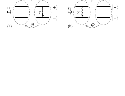
Figure 1: Schemes corresponding to the system energy levels and environment states. (a) First case, Eq. (7). (b) Second case, Eq. (8). In both schemes, $\Omega$ measures the system-laser coupling, $\gamma$ is the system decay rate, while $\phi$ and $\varphi$ are the transitions rates between the two bath-states $\left|a_{\mathrm{0}}\right\rangle$ and $\left|a_{1}\right\rangle.$

The operator $T$ introduces the natural decay of the system $(\left|+\right\rangle\rightsquigarrow\left|-\right\rangle)$ taking into account its dependence on the bath-states. In the first case [Eq. (7)] it reads

$$T=\sigma\otimes\left|a_{1}\right\rangle\left\langle a_{1}\right|,$$ (73)

while in the second case [Eq. (8)] becomes

$$T=\sigma\otimes\left|a_{\mathrm{0}}\right\rangle\left\langle a_{\mathrm{0}}\right|.$$ (74)

Consistently, the lowering system operator reads $\sigma=\left|-\right\rangle\left\langle+\right|.$ The decay rate is $\gamma.$

Figure 2: Waiting time distributions $w_{\mathrm{in}}(t)$ [Eq. (60)] (solid black line) and $w(t)$ [Eq. (59)] (dotted black line) corresponding to Fig. 1(a) (first case). The inset shows the associated survival probabilities $P_{0}^{\mathrm{in}}(t)$ and $P_{0}(t)$ respectively, Eq. (65). The parameters are $\Omega/\gamma=0.15,$ and $\phi/\gamma=\varphi/\gamma=0.01.$ The initial system state is $\rho_{0}^{s}=\left|-\right\rangle\left\langle-\right|.$ For the same parameter values, the statistical objects of the second case, Fig. 1(b), are given by the plots of $w(t)$ and $P_{0}(t).$

We remark that in both cases, the evolution defined by Eq. (IV) cannot be mapped with the example worked out in Ref. OneChannel . In fact, although the Lindblad contributions are similar, in that case the system-ancilla coupling is Hamiltonian. Hence, the ancilla dynamics is quantum while here it is classical (ancilla populations and coherences are not coupled).

IV.1 Non-Markovian density matrix evolution

In agreement with the previous analysis, the initial condition is taken as [Eq. (21)]

$$\rho_{0}^{sa}=\rho_{0}^{s}\otimes\left|a_{\mathrm{0}}\right\rangle\left\langle a_{\mathrm{0}}\right|,$$ (75)

where $\rho_{0}^{s}$ is an arbitrary system state. Hence, the ancilla begins in its lower state. Taking into account the previous definitions and the results of Sec. II it is straightforward to write down the non-Markovian system density matrix evolution. In the first case, it is given by the non-Markovian master equation (26) defined with the exponential kernel (36), while in the second case, Eq. (32) with the kernel (37). In both cases the superoperator $\mathcal{L}_{s}$ and $\mathcal{C}_{s}$ follows from Eq. (IV). $\mathcal{L}_{s}$ reads

$$\mathcal{L}_{s}[\rho]=-i\frac{\Omega}{2}[\sigma_{x},\rho],$$ (76)

while dissipative effects are introduced by

$$\mathcal{C}_{s}[\rho]=\frac{\gamma}{2}([\sigma,\rho\sigma^{\dagger}]+[\sigma\rho,\sigma^{\dagger}]).$$ (77)

By writing $(d/dt)\rho_{t}^{s}=(\mathcal{L}_{s}+\mathcal{C}_{s})\rho_{t}^{s}$ these superoperators recover the dynamics of a Markovian fluorescent two-level system carmichaelbook ; breuerbook . The dependence of the decay rate $\gamma$ on the bath-states (Fig. 1) introduce the non-Markovian effects that lead to the evolutions (26) and (32). Notice that in the first case the Markovian dynamics is recovered for $\phi\rightarrow\infty,$ $\varphi=0,$ while in the second case for $\phi\rightarrow 0,$ and any $\varphi$ (see Fig. 1). It is simple to cheek that these Markovian limits are achieved by the non-Markovian evolutions (26) and (32) after taking into account the kernel definitions Eqs. (36) and (37) respectively.

IV.2 Measurement realizations

In concordance with the dissipative structure (77), we assume that the measurement apparatus detects the optical transitions of the system. It is simple to check that $\mathcal{C}_{s}$ has the renewal structure corresponding to Eqs. (39) and (40). The post measurement state [Eq. (45)] is $\mathcal{M}[\rho]=\left|-\right\rangle\left\langle-\right|.$ Hence, after each detection event the system collapses to its ground state.

In the first case, the statistics of the time interval between detection events is defined by the waiting time densities $w_{\mathrm{in}}(t)$ [Eq. (60)] and $w(t)$ [Eq. (59)]. In Fig. 2 we plotted these objects and their associated survival probabilities $P_{0}^{\mathrm{in}}(t)$ and $P_{0}(t)$ respectively, Eq. (65). All these statistical objects can be obtained in an exact analytical way in the Laplace domain. Nevertheless, contrary to the Markovian case carmichael ; bartano , here the time dependence can only be obtained with numerical methods. In fact, Laplace inversion via Cauchy’s residue theorem, for arbitrary parameter values, involves roots of a sextic polynomial (degree 6) in the Laplace variable $u.$ This feature is induced by the underlying classical transitions of the bath-states, which in turn lead to dynamical behaviors that depart from the Markovian case.

In the Markovian limit described previously, for $\rho_{0}^{s}=\left|-\right\rangle\left\langle-\right|,$ follows the analytical results $w_{\mathrm{in}}(t)=w(t)=4\gamma\Omega^{2}\exp(-\gamma t/2)[\sinh(\Phi t/4)/\Phi]^{2},$ with the “frequency” $\Phi\equiv\sqrt{\gamma^{2}-4\Omega^{2}}.$ This analytical expression was obtained previously in Refs. carmichael ; bartano . For $\Omega^{2}>\gamma^{2}/4,$ $w_{\mathrm{in}}(t)$ develops an oscillatory behavior. Nevertheless, in the non-Markovian case corresponding to Fig. 2, $w_{\mathrm{in}}(t)$ develops oscillations even when $\Omega^{2}<\gamma^{2}/4.$ This feature occurs because here the system is able to perform Rabi oscillations before the first bath transition happens $\left|a_{\mathrm{0}}\right\rangle\overset{\phi}{\rightarrow}\left|a_{1}\right\rangle$ (see Fig. 1), that is, oscillations in $w_{\mathrm{in}}(t)$ appear under the condition $\Omega>\phi.$ On the other hand, in Fig. 2 $w(t)$ does not oscillate and approach the Markovian solution carmichael ; bartano . This last feature occurs whenever the system is able to perform many optical transitions before the configurational bath change $\left|a_{1}\right\rangle\overset{\varphi}{\rightarrow}\left|a_{\mathrm{0}}\right\rangle$ happens. Hence, $w(t)$ approaches the Markovian solution when $\bar{\tau}^{-1}>\varphi,$ where $\bar{\tau}$ is the average time between consecutive emissions in the Markovian case, $\bar{\tau}^{-1}=\gamma\Omega^{2}/(\gamma^{2}+2\Omega^{2})$ plenio ; carmichaelbook . For the parameters of Fig. 2 it follows $\bar{\tau}^{-1}/\varphi\simeq 2.15>1.$ In general, for arbitrary parameters values, $w(t)$ cannot be related to the waiting time density of the Markovian case.

For the chosen parameter values, $\phi=\varphi,$ and initial condition, $\rho_{0}^{s}=\left|-\right\rangle\left\langle-\right|,$ it is simple to realize that the statistics corresponding to the second case is completely determined by the waiting time density $w(t)$ and survival probability $P_{0}(t)$ corresponding to the first case (Fig. 2).

Figure 3: Stochastic realizations corresponding to the first (a) and second case (b). The parameters are the same than in Fig. 2.

On the basis of the survival probabilities it is possible to generate the measurements realizations corresponding to $\rho_{\mathrm{st}}^{s}(t),$ Eq. (66). In Fig. 3, we show a realization of $\left\langle+\right|\rho_{\mathrm{st}}^{s}(t)\left|+\right\rangle.$ Each detection event corresponds to the collapse to zero of this population. In agreement with previous analysis, in the first case [Fig. 3(a)] the conditional dynamics of the first event [Eqs. (63) and (49)] is different of the subsequent ones [Eqs. (63) and (55)]. In contrast, in the realizations of the second case [Fig. 3(b)] the conditional dynamics is always the same. Due to the chosen parameter values $(\phi=\varphi)$ it also corresponds to the conditional dynamics of the first case after the first event.

In Fig. 4 we plot the upper population $\left\langle+\right|\rho_{t}^{s}\left|+\right\rangle$ obtained from the non-Markovian evolutions Eqs. (26) and (32) with the kernels (36) and (37) respectively. Furthermore, we plotted the behavior of $\left\langle+\right|\bar{\rho}_{\mathrm{st}}^{s}(t)\left|+\right\rangle$ obtained by averaging $3\times 10^{2}$ realizations shown in Fig. 3. Consistently, in both cases the master equations fit the average ensemble behavior. This fact shows the consistence of the non-Markovian quantum jump approach developed in Sec. III. Furthermore, we checked that the same analytical (Laplace domain) and numerical results (Fig. 2 to Fig. 4) are obtained by tracing out the bipartite Markovian representation (see Appendix).

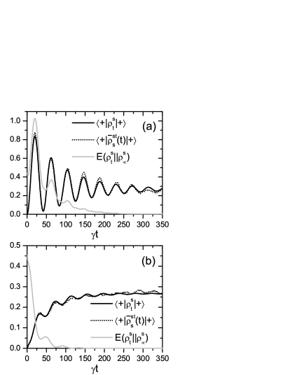
Figure 4: Exact solution (black full line) for the upper population $\left\langle+\right|\rho_{t}^{s}\left|+\right\rangle.$ The dotted (noisy) line correspond to an average over $3\times 10^{2}$ realizations of $\left\langle+\right|\rho_{\mathrm{st}}^{s}(t)\left|+\right\rangle$ shown in Fig. 3. The solid gray line corresponds to the relative entropy $E(\rho_{t}^{s}||\rho_{\infty}^{s}),$ Eq. (78). (a) First case, defined by the master Eq. (26) with the exponential kernel (36). (b) Second case, master Eq. (32) with the kernel (37).

IV.3 Environment-to-system backflow of information

In Ref. piilo it was found that both dynamics (1) and (3) do not lead to “genuine” non-Markovian effects such as an environment-to-system backflow of information NoMeasure . In the present approach, that result is completely expectable. In fact, when $[\mathcal{L}_{s},\mathcal{C}_{s}]=0,$ from Eqs. (7) and (8) (take $\mathcal{L}_{s}\rightarrow 0)$ it is simple to realize that the different environment states only turn-on and turn-off the Markovian dynamics defined by $\mathcal{C}_{s}.$ Thus, it is impossible to get an information backflow. In the example of this section that situation corresponds to take $\Omega=0$ in Fig. 1. Nevertheless, when $[\mathcal{L}_{s},\mathcal{C}_{s}]\neq 0,$ the bath fluctuations lead to a switching between two “different” Markovian dynamics. Below we show that this underlying effect may lead to a backflow of information in the generalized dynamics defined by Eqs. (7) and (8).

For simplicity, as a witness or detector of the backflow of information we consider the relative entropy with respect to the stationary state NoMeasure

$$E(\rho_{t}^{s}||\rho_{\infty}^{s})=\mathrm{Tr}_{s}[\rho_{t}^{s}(\ln_{2}\rho_{t}^{s}-\ln_{2}\rho_{\infty}^{s})],$$ (78)

where $\rho_{\infty}^{s}=\lim_{t\rightarrow\infty}\rho_{t}^{s}.$ Hence, the backflow of information occurs if there exist times $t_{2}>t_{1}$ such that $E(\rho_{t_{2}}^{s}||\rho_{\infty}^{s})>E(\rho_{t_{1}}^{s}||\rho_{\infty}^{s})$ OneChannel ; Embedding .

By working in a Laplace domain, the stationary states corresponding to the schemes of Fig. 1 can be obtained in an exact way. As $\rho_{\infty}^{s}$ does not depend on the (system-bath) initial condition, it follows the property $\rho_{\infty}^{s}(\phi,\varphi)|_{\mathrm{I}}=\rho_{\infty}^{s}(\varphi,\phi)|_{\mathrm{II}},$ where $\rho_{\infty}^{s}(\phi,\varphi)|_{\mathrm{I}}$ is the stationary state of the first case with parameters $(\phi,\varphi),$ while $\rho_{\infty}^{s}(\varphi,\phi)|_{\mathrm{II}}$ is the stationary of the second case where the role of the parameters is interchanged, that is, $\varphi\leftrightarrow\phi.$

For each case, in Fig. 4 we also plotted the relative entropy (78) (solid gray lines). $E(\rho_{t}^{s}||\rho_{\infty}^{s})$ develops “revivals” showing that in both cases the dynamics lead to a backflow of information. Consistently with the analysis of Ref. piilo this phenomenon only appears if $\Omega\neq 0,$ that is, when the dissipative and unitary contributions do not commutate.

V Summary and conclusions

In this paper we established a solid physical basis for an alternative derivation and understanding of two extensively studied non-Markovian master equations. As underlying “microscopic dynamics” we utilized a system coupled to an environment that is able to develop classical self-fluctuations which in turn modify the system dissipative dynamics, Eqs. (7) and (8). From a bipartite system-ancilla representation, Eq. (12), and by means of a projector technique, we obtained the non-Markovian master equations (26) and (32), which represent one of the main results of this work. If the unitary and dissipative superoperators commutate, Shabani-Lidar equation, Eq. (1), and its associated evolution, Eq. (3), are recovered respectively.

In contrast with phenomenological approaches, here the statistical behavior of the environment fluctuations completely determine the memory functions, Eqs. (28) and (33). The paradigmatic case of exponential kernels arises when the environment has only two configurational states, Eqs. (36) and (37). By construction, kernels associated to an arbitrary number of bath-states, Eq. (5), also guaranty the completely positive condition of the solution map for any value of the underlying characteristic parameters.

On the basis of the bipartite representation, we found the conditions under which the system dynamics can be unravelled in terms of an ensemble of measurement realizations whose dynamics can be written in a closed way, that is, without involving explicit information about the configurational bath-states. Eq. (26) can be unravelled when the bath has two configurational states, while for Eq. (32) this condition is not necessary. Nevertheless, in both cases a renewal condition is required. As in the standard Markovian case, the realizations consist of periods where the evolution is smooth and non-unitary, while at the detection times the system suddenly collapses to the same resetting state. The non-Markovian features of the dynamics are present in the conditional dynamics between jumps, which in turn may be different from the first interval. The unravelling of the system dynamics in terms of (closed) measurement trajectories remains as an open problem when the previous conditions are not satisfied.

The consistence of the previous findings has been explicitly demonstrated by studying the dynamics of a two-level system whose decay is modulated by the environment states. This example allowed us to show that a backflow of information from the environment to the system appears in both master equations. Therefore, the absence of this phenomenon for the particular situation analyzed in Ref. piilo is not a general property of the dynamics. In fact, we demonstrated that the backflow of information may occurs only when the system unitary dynamics does not commutate with the dissipative one.

In summary, the formalism presented here gives a clear physical interpretation of some phenomenological aspects that appears in the formulation of the studied non-Markovian quantum master equations. These results are of help for understanding and modeling the great variety of phenomena emerging in presence of memory effects.

Appendix A Quantum jumps from the bipartite representation

The properties of the non-Markovian quantum jump approach developed in Sec. III can be derived from a standard Markovian quantum jump approach formulated on the basis of the bipartite dynamics (12).

A.1 Conditions for getting a closed measurement ensemble

Firstly, we derive the conditions under which the non-Markovian dynamics (26) and (32) can be unravelled in terms of an ensemble of trajectories whose dynamics can be written in a closed form, that is, without involving in an explicit way the ancilla (bath) states. As mentioned in Section III, these results rely on the bipartite representation of the non-Markovian system dynamics.

As demonstrated in Ref. OneChannel , a “closed quantum jump approach” can be formulated for the system of interest if the bipartite dynamics Eq. (12) fulfill the conditions

$$\mathrm{Tr}_{a}[\mathbb{M}\rho_{sa}]=\mathcal{M}[\mathrm{Tr}_{a}(\rho_{sa})],\ \ \ \ \ \ \ \ \ \ \ \ \mathrm{Tr}_{s}[\mathbb{M}\rho_{sa}]=\bar{\rho}_{a}.$$ (79)

Here, $\mathbb{M}$ is the bipartite transformation associated to each detection event and $\bar{\rho}_{a}$ is an arbitrary ancilla state. The first condition guarantees that each measurement event in the bipartite space can also be read as a measurement transformation $\mathcal{M}$ in the system Hilbert space. The second condition guarantees that the conditional system dynamics between detection events does not depend explicitly on the ancilla state OneChannel . Therefore, under the previous conditions, the system measurement dynamics has the same structure (non-unitary conditional dynamics followed by state collapses) than in the Markovian case.

Assuming that the measurement apparatus is sensitive to all system transitions defined by the operators $V_{\alpha}$ [Eq. (2)], it follows breuerbook

$$\mathcal{M}[\rho]=\frac{\sum\nolimits_{\alpha}\gamma_{\alpha}V_{\alpha}\rho V_{\alpha}^{{\dagger}}}{\mathrm{Tr}_{s}[\sum\nolimits_{\alpha}\gamma_{\alpha}V_{\alpha}^{{\dagger}}V_{\alpha}\rho]}.$$ (80)

In the first case, from Eqs. (12) and (14), the bipartite transformation $\mathbb{M}$ reads

$$\mathbb{M}[\rho]=\frac{\sum\nolimits_{\alpha,i}^{{}^{\prime}}\gamma_{\alpha}T_{\alpha i}\rho T_{\alpha i}^{{\dagger}}}{\mathrm{Tr}_{sa}[\sum\nolimits_{\alpha,i}^{{}^{\prime}}\gamma_{\alpha}T_{\alpha i}^{{\dagger}}T_{\alpha i}\rho]},$$ (81)

where $T_{\alpha i}=V_{\alpha}\otimes\left|a_{i}\right\rangle\left\langle a_{i}\right|,$ Eq. (15). On the other hand, in the second case, from Eqs. (12) and (16), it becomes

$$\mathbb{M}[\rho]=\frac{\sum\nolimits_{\alpha}\gamma_{\alpha}T_{\alpha 0}\rho T_{\alpha 0}^{{\dagger}}}{\mathrm{Tr}_{sa}[\sum\nolimits_{\alpha}\gamma_{\alpha}T_{\alpha 0}^{{\dagger}}T_{\alpha 0}\rho]},$$ (82)

where $T_{\alpha 0}=V_{\alpha}\otimes\left|a_{\mathrm{0}}\right\rangle\left\langle a_{\mathrm{0}}\right|,$ Eq. (17). For arbitrary set of operators $\{V_{\alpha}\},$ neither Eq. (81) nor Eq (82) fulfill the conditions (79).

When the operators $\{V_{\alpha}\}$ lead to a renewal measurement process [Eq. (39)], Eq. (81) becomes

$$\mathbb{M}[\rho]=\bar{\rho}_{s}\otimes\frac{\sum\nolimits_{i}^{{}^{\prime}}\left\langle ua_{i}\right|\rho\left|ua_{i}\right\rangle\Pi_{i}}{\sum\nolimits_{i}^{{}^{\prime}}\left\langle ua_{i}\right|\rho\left|ua_{i}\right\rangle}.$$ (83)

This structure does not satisfy the condition (79). Nevertheless, when the ancilla Hilbert space is bidimensional, $i=0,1,$ given that $\sum\nolimits_{i}^{{}^{\prime}}$ excludes the contribution $i=0,$ it follows

$$\mathbb{M}[\rho]=\bar{\rho}_{s}\otimes\Pi_{1},$$ (84)

which evidently satisfies Eq. (79). $\bar{\rho}_{s}$ is given by Eq. (43). Therefore, only when the kernel is an exponential one, Eq. (36), a closed system (renewal) measurement dynamics can be associated with the non-Markovian evolution (26).

In the second case, Eq. (82) with the operators (39) becomes

$$\mathbb{M}[\rho] = \mathcal{M}[\left\langle a_{\mathrm{0}}\right|\rho_{sa}\left|a_{\mathrm{0}}\right\rangle]\otimes\Pi_{0},$$ (85a)

$$= \bar{\rho}_{s}\otimes\Pi_{0}.$$ (85b)

Independently of the ancilla dimension the closure conditions (79) are satisfied. Thus, under the renewal condition the non-Markovian evolution (32) can be unravelled independently of the ancilla dynamics, that is, for arbitrary kernels with the structure defined by Eq. (33).

A.2 Conditional dynamics

In the bipartite description, the non-Markovian conditional system dynamic can be obtained by tracing out the joint system-ancilla dynamics. Therefore, it is possible to obtain alternative expressions for the system conditional propagators written in terms of the bipartite dynamics.

In the first case, the conditional propagator $\mathcal{\hat{T}}(u),$ Eq. (49), from Eqs. (12) and (14) can also be written as

$$\mathcal{\hat{T}}(u)[\rho]=\mathrm{Tr}_{a}\Big{[}\frac{1}{u-(\mathcal{L}_{s}+\mathcal{L}_{a}+\mathbb{D)}}(\rho\otimes\Pi_{\mathrm{0}})\Big{]},$$ (86)

where the bipartite initial condition (21) was taken into account. The propagator $\mathcal{\hat{T}}^{\prime}(u),$ Eq. (55), taking into account the resetting state (84) becomes

$$\mathcal{\hat{T}}^{\prime}(u)[\rho]=\mathrm{Tr}_{a}\Big{[}\frac{1}{u-(\mathcal{L}_{s}+\mathcal{L}_{a}+\mathbb{D)}}(\rho\otimes\Pi_{\mathrm{1}})\Big{]}.$$ (87)

Therefore, the difference between both propagators arises from a different ancilla initial condition. In the previous two equations, the bipartite superoperator $\mathbb{D}$ is defined by the expression $\mathcal{C}_{sa}=\mathbb{D}+\mathbb{J},$ where $\mathcal{C}_{sa}$ is given by Eq. (14) and $\mathbb{J}$ defines the bipartite measurement transformation $\mathbb{M}[\rho]=\mathbb{J}[\rho]/\mathrm{Tr}_{sa}[\mathbb{J}\rho],$ Eq. (81). Therefore, it reads

$$\mathbb{D}[\rho] = -\frac{1}{2}\sum\nolimits_{i,\alpha}^{{}^{\prime}}\gamma_{\alpha}\{T_{\alpha i}^{{\dagger}}T_{\alpha i},\rho\}_{+},$$ (88a)

$$= -\frac{1}{2}\sum\nolimits_{\alpha}\gamma_{\alpha}\{V_{\alpha}^{{\dagger}}V_{\alpha}\otimes\Pi_{\mathrm{1}},\rho\}_{+}.$$ (88b)

In the second line, as well as in the previous two equations for $$\mathcal{\hat{T}}(u) \mathcal{\hat{T}}^{\prime}(u),$$ and we used that the configurational bath space is two-dimensional.

In the second case, both propagators are the same, $\mathcal{\hat{T}}^{\prime}(u)=\mathcal{\hat{T}}(u).$ From Eqs. (12) and (16), $\mathcal{\hat{T}}(u)$ can be written as in Eq. (86) with the superoperator $\mathbb{D}$ defined by the expression

$$\mathbb{D}[\rho] \mathbb{=} -\frac{1}{2}\sum\nolimits_{\alpha}\gamma_{\alpha}\{T_{\alpha 0}^{{\dagger}}T_{\alpha 0},\rho\}_{+},$$ (89a)

$$= -\frac{1}{2}\sum\nolimits_{\alpha}\gamma_{\alpha}\{V_{\alpha}^{{\dagger}}V_{\alpha}\otimes\Pi_{\mathrm{0}},\rho\}_{+}.$$ (89b)

In this case, this definition is valid for an arbitrary number of bath-states.

The previous expressions for the conditional propagators can be solved in an exact way in the Laplace domain. They also provide an alternative and equivalent way for getting statistical objects such as the survival probabilities Eq. (65), or equivalently their associated waiting time densities, Eqs. (59) and (60).

References

• (1) R. Alicki and K. Lendi, Quantum Dynamical Semigroups and Applications, Lecture Notes in Physics 286 (Springer, Berlin, 1987).
• (2) H. P. Breuer and F. Petruccione, The theory of open quantum systems, Oxford University press (2002).
• (3) F. Haake, in Statistical Treatment of Open Systems by Generalized Master Equations, (Springer, 1973).
• (4) S. M. Barnett and S. Stenholm, Phys. Rev. A 64, 033808 (2001).
• (5) A. A. Budini, Phys. Rev. A 69, 042107 (2004); A. A. Budini and P. Grigolini, Phys. Rev. A 80, 022103 (2009).
• (6) F. Giraldi and F. Petruccione, Open Syst. Inf. Dyn. 19, 1250011 (2012); C. Pellegrini and F. Petruccione, J. Phys. A Math. Theor. 42, 425304 (2009).
• (7) B. Vacchini, Phys. Rev. A 87, 030101(R) (2013).
• (8) F. Ciccarello, G. M. Palma, and V. Giovanneti, Phys. Rev. A 87, 040103(R) (2013); F. Ciccarello and V. Giovannetti, Phys. Scr. T153, 014010 (2013); T. Rybar, S. N. Filippov, M. Ziman, and V. Buzek, J. Phys. B 45, 154006 (2012).
• (9) J. Wilkie, Phys. Rev. E 62, 8808 (2000); J. Wilkie, J. Chem. Phys. 114, 7736 (2001); ibid 115, 10335 (2001); J. Wilkie and Y. M. Wong, J. Phys. A 42, 015006 (2008).
• (10) J. Salo, S. M. Barnett, and S. Stenholm, Op. Comm. 259, 772 (2006).
• (11) S. Daffer, K. Wodkiewicz, J. D. Cresser, and J. K. McIver, Phys. Rev. A 70, 010304(R) (2004); E. Anderson, J. D. Cresser, and  M. J. V. Hall, J. Mod. Optics 54, 1695 (2007).
• (12) A. Shabani and D. A. Lidar, Phys. Rev. A 71, 020101(R) (2005).
• (13) S. Maniscalco and F. Petruccione, Phys. Rev. A 73, 012111 (2006); 75, 059905 (2007).
• (14) S. Maniscalco, Phys. Rev. A 75, 062103 (2007).
• (15) L. Mazzola, E. M. Laine, H. P. Breuer, S. Maniscalco, and J. Piilo, Phys. Rev. A 81, 062120 (2010).
• (16) S. Campbell, A. Smirne, L. Mazzola, N. Lo Gullo, B. Vacchini, Th. Busch, and M. Paternostro, Phys. Rev. A 85, 032120 (2012).
• (17) A. A. Budini, Phys. Rev. A 74, 053815 (2006); Phys. Rev. E 72, 056106 (2005); A. A. Budini and H. Schomerus, J. Phys. A 38, 9251, (2005).
• (18) B. Vacchini, Phys. Rev. A 78, 022112 (2008).
• (19) H. P. Breuer and B. Vacchini, Phys. Rev. Lett. 101, 140402 (2008); H. P. Breuer and B. Vacchini, Phys. Rev. E 79, 041147 (2009).
• (20) D. Chruscinski and A. Kossakowski, Phys. Rev. Lett. 104, 070406 (2010); A. Kossakovski and R. Rebolledo, Open Systems & Information Dynamics 14, 265 (2007); ibid, 15, 135 (2008); D. Chruscinski, A. Kossakowski, and S. Pascazio, Phys. Rev. A 81, 032101 (2010).
• (21) H. P. Breuer, E. M. Laine, and J. Piilo, Phys. Rev. Lett. 103, 210401 (2009); E. M. Laine, J. Piilo, and H. P. Breuer, Phys. Rev. A 81, 062115 (2010); D. Chruscinski, A. Kossakowski, and A. Rivas, Phys. Rev. A 83, 052128 (2011); B. Vacchini, A. Smirne, E. M. Laine, J. Piilo, and H. P. Breuer, New J. Phys. 13, 093004 (2011); B. Vacchini, J. Phys. B 45, 154007 (2012); C. Addis, P. Haikka, S. McEndoo, C. Macchiavello, and S. Maniscalco, Phys. Rev. A 87, 052109 (2013).
• (22) L. Diosi, Phys. Rev. Lett. 100, 080401 (2008); H. M. Wiseman and J. M. Gambetta, Phys. Rev. Lett. 101, 140401 (2008).
• (23) J. Piilo, S. Maniscalco, K. Härkönen, and K. A. Suominen, Phys. Rev. Lett. 100, 180402 (2008); K. Luoma, K. Härkönen, S. Maniscalco, K. A. Suominen, and J. Piilo, Phys. Rev. A 86, 022102 (2012); E. M. Laine, K. Luoma, and J. Piilo, J. Phys. B 45, 154004 (2012); J. Piilo, K. Härkönen, S. Maniscalco, and K. A. Suominen, Phys. Rev. E 79, 062112 (2009).
• (24) A. A. Budini, Phys. Rev. A 73, 061802(R) (2006); J. Chem. Phys. 126, 054101 (2007); Phys. Rev. A 76, 023825 (2007); J. Phys. B 40, 2671 (2007).
• (25) M. Moodley and F. Petruccione, Phys. Rev. A 79, 042103 (2009); X. L. Huang, H. Y. Sun, and X. X. Yi, Phys. Rev. E 78, 041107 (2008).
• (26) A. Barchielli, C. Pellegrini, and F. Petruccione, Phys. Rev. A 86, 063814 (2012); A. Barchielli, C. Pellegrini, J. Math. Phys. 51, 112104 (2010); A. Barchielli and M. Gregoratti, Phil. Trans. R. Soc. A 370, 5364 (2012); A. Barchielli, C. Pellegrini, and F. Petruccione, Eur. Phys. Lett. 91, 24001 (2010).
• (27) A. A. Budini, Phys. Rev. A 88, 012124 (2013).
• (28) A. A. Budini, Phys. Rev. A 88, 032115 (2013).
• (29) A. Barchielli and M. Gregoratti, Quantum Trajectories and Measurements in Continuous time—The diffusive case, Lectures Notes in Physics Vol. 782 (Springer, Berlin, 2009).
• (30) M. B. Plenio and P. L. Knight, Rev. Mod. Phys. 70, 101 (1998).
• (31) H. J. Carmichael, An Open Systems Approach to Quantum Optics, Vol. M18 of Lecture Notes in Physics (Springer, Berlin, 1993).
• (32) H. J. Carmichael, S. Singh, R. Vyas, and P. R. Rice, Phys. Rev. A 39, 1200 (1989); G. C. Hegerfeldt, Phys. Rev. A 47, 449 (1993).
• (33) A. Barchielli, Some stochastic differential equations in quantum optics and measurement theory: the case of counting processes. In L. Diòsi, B. Lukàcs (eds.), Stochastic Evolution of Quantum States in Open Systems and in Measurement Processes (World Scientific, Singapore, 1994), pp. 1–14.
• (34) E. Barkai, Y. Jung, and R. Silbey, Annu. Rev. Phys. Chem. 55, 457 (2004); M. Lippitz, F. Kulzer, and M. Orrit, Chem. Phys. Chem. 6, 770 (2005); Y. Jung, E. Barkai, and R.J. Silbey, J. Chem. Phys. 117, 10980 (2002).
• (35) A. A. Budini, Phys. Rev. A 79, 043804 (2009); J. Phys. B 43, 115501 (2010).
• (36) N. G. van Kampen, Stochastic Processes in Physics and Chemistry, (North-Holland, Amsterdam, 1992), Chap. XVII, Sect. 7 (internal noise).