Scalable Rejection Sampling for Bayesian Hierarchical Models

Abstract

Bayesian hierarchical modeling is a popular approach to capturing unobserved heterogeneity across individual units. However, standard estimation methods such as Markov chain Monte Carlo (MCMC) can be impracticable for modeling outcomes from a large number of units. We develop a new method to sample from posterior distributions of Bayesian models, without using MCMC. Samples are independent, so they can be collected in parallel, and we do not need to be concerned with issues like chain convergence and autocorrelation. The algorithm is scalable under the weak assumption that individual units are conditionally independent, making it applicable for large datasets. It can also be used to compute marginal likelihoods.

Forthcoming in Marketing Science
Special Issue on Big Data: Integrating Marketing, Statistics and Computer Science

1 Introduction

In 1970, John D. C. Little famously wrote: “The big problem with management science models is that managers practically never use them. There have been a few applications, of course, but the practice is a pallid picture of the promise” [29]. The same may be true today about Bayesian estimation of hierarchical probability models. The impact Bayesian methods have had on academic research across multiple disciplines in the managerial, social and natural sciences is undeniable. Marketing, in particular, has benefited from Bayesian methods because of their natural suitability for capturing heterogeneity in customer types and tastes [38]. But further diffusion of Bayesian methods is constrained by a scalability problem. As the size and complexity of data sources for both research and commercial purposes grows, the impracticality of simulation-based Bayesian methods for estimating parameters of a general class of hierarchical models becomes increasingly salient [1].

The problem is not with the Bayesian approach itself, but with the most familiar methods of simulating from the posterior distributions of the parameters. Without question, the resurgence of Bayesian ideas is due to the popularity of Markov chain Monte Carlo (MCMC), which was introduced to statistical researchers by [21] via the Gibbs sampler. MCMC estimation involves iteratively sampling from the marginal posterior distributions of blocks of parameters. Only after some unknown (and theoretically infinite) number of iterations will the algorithm generate samples from the correct distributions; earlier samples are discarded. The Bayesian computational literature has exploded with numerous methods for generating valid and efficient MCMC algorithms. It would be difficult to list all of them here, so we refer the reader to [23, 11, 39] and [9], and the hundreds of references therein.

Despite the justifiable success MCMC has enjoyed, there remains the question of whether a particular chain has run long enough that we can start collecting samples for estimation (or, colloquially, whether the chain has “converged” to the target distribution). This is a particular problem for hierarchical models in which each heterogeneous unit is characterized by its own set of parameters. For example, each household in a customer dataset might have its own preferences for product attributes. Both the number of parameters and the cycle time for each MCMC iteration grow with the size of the dataset. Also, if the data represent outcomes of multiple interdependent processes (such as the timing and magnitude of purchases), both the posterior parameters and successive MCMC samples tend to be correlated, requiring a larger, yet unknown, number of iterations. We believe that the most important reason Bayesian methods have not been embraced “in the field” nearly as much as classical approaches is that they are difficult and expensive to implement routinely using MCMC, even with semi-automated software procedures. Practitioners simply do not have an academician’s luxury of letting an MCMC chain run for days or weeks with no guarantee that the chain has converged to produce “correct” answers at the end of the process.

With recent developments in multiple core processing and distributed computing systems, it is reasonable to look to parallel computing technology as a solution to the convergence problem. However, each MCMC cycle depends on the outcome of the previous one, so we cannot collect posterior samples in parallel by allocating the work across distributed processing cores. Using parallel processors to generate one draw from a target distribution, or running several MCMC chains in parallel, is not the same as generating all the required independent samples in parallel. Hence, extant parallel MCMC methods are also subject to the same pesky question of convergence; indeed, now one has to ensure that all of the parallel chains have converged. On the other hand, non-MCMC methods like rejection sampling have the advantage of being able to generate samples from the correct target posterior in parallel, but these methods are beset with their own set of implementation issues. For instance, the inability to find efficient “envelope” distributions renders standard rejection sampling almost impractical for all but the smallest problems.

In this paper, we propose a solution to sample from Bayesian parametric, hierarchical models that is inspired by two pre-MCMC approaches: rejection sampling, and sampling from a multivariate normal (MVN) approximation around the posterior mode. Our contribution is an algorithm that recasts traditional rejection sampling in a way that circumvents the difficulties associated with these two approaches. The algorithm requires that one be able to compute the unnormalized log posterior of the parameters (or a good approximation of it); that the posterior distribution is bounded from above over the parameter space; and that available computing resources can locate any local maxima of the log posterior. There is no need to derive conditional posterior distributions (as with blockwise Gibbs sampling), and there are no conjugacy requirements.

We present the details of our method in Section 2, and in Section 3, we share some examples that demonstrate the method’s effectiveness. In broad strokes, the method involves scaling an MVN distribution around the mode, and using that distribution as the source of proposal draws for the modified rejection algorithm. At first glance, one might think that finding the posterior mode, and sampling from an MVN, are themselves intractable tasks in large dimensions. After all, the Hessian of the log posterior density, which grows quadratically with the number of parameters, is an important determinant of the efficiency of both MVN sampling and nonlinear optimization. Fortunately, several independent software development projects have spawned novel, freely available numerical computation tools that, when used together, allow our method to scale. In Section 4, we explain how to manage this scalability issue, and show that the complexity of our method scales approximately linearly with the number of heterogeneous units.

Another complication of Bayesian methods is the estimation of the marginal likelihood of the data. The marginal likelihood is the probability of observing the data under the proposed model, which can be used as a metric for model comparison. Except in rare special cases, computing the marginal likelihood involves numerically integrating over all of the prior parameters; note that we consider hyperpriors to be part of the data in this case. In Section 5, we explain how to estimate the marginal likelihood as a by-product of our method.

In Section 6, we discuss key implementation issues, and identify some relevant software tools. We also discuss limitations of our approach. We are not claiming that our method should replace MCMC in all cases. It may not be practical for models with discrete parameters, a very large number of modes, or for which computing the log posterior density itself is difficult. The method does not require that the model be hierarchical, or that the conditional independence assumption holds, but without those assumptions, it will not be as scalable. Nevertheless, many models of the kind researchers encounter could be properly estimated using our method, at least relative to the effort involved in using MCMC. Like MCMC and other non-MCMC methods, our method is another useful algorithm in the researcher’s and practitioner’s toolkits.

2 Method details

2.1 Theoretical basis

The goal is to sample a parameter vector $\theta$ from a posterior density $\pi(\theta|y)$, where $\pi(\theta)$ is the prior on $\theta$, $f(y|\theta)$ is the data likelihood conditional on $\theta$, and $\mathcal{L}(y)$ is the marginal likelihood of the data. Therefore,

$$\pi(\theta|y)=\frac{f(y|\theta)\pi(\theta)}{\mathcal{L}(y)}=\frac{\mathcal{D}(\theta,y)}{\mathcal{L}(y)}$$ (1)

where $\mathcal{D}(\theta,y)$ is the joint density of the data and the parameters (of the unnormalized posterior density). In a marketing research context, under the conditional independence assumption, the likelihood can be factored as

$$f(y|\theta)=\prod_{i=1}^{N}f_{i}\left(y_{i}|\beta_{i},\alpha\right)$$ (2)

where $i$ indexes households. Each $y_{i}$ is a vector of observed data, each $\beta_{i}$ is a vector of heterogeneous parameters, and $\alpha$ is a vector of homogeneous population-level parameters. The $\beta_{i}$ are distributed across the population of households according to a mixing distribution $\pi(\beta_{i}|\alpha)$, which also serves as the prior on each $\beta_{i}$. The elements of $\alpha$ may influence either the household-level data likelihoods, or the mixing distribution (or both). In this example, $\theta$ includes all $\beta_{1}\mathellipsis\beta_{N}$ and all elements of $\alpha$. The prior itself can be factored as

$$\pi(\theta)=\prod_{i=1}^{N}\pi_{i}(\beta_{i}|\alpha)\times\pi(\alpha).$$ (3)

Let $\theta^{*}$ be the mode of $\mathcal{D}(\theta,y)$, which is also the mode of $\pi(\theta|y)$, since $\mathcal{L}(y)$ is a constant that does not depend on $\theta$. One will probably use some kind of iterative numerical optimizer to find $\theta^{*}$, such as a quasi-Newton line search or trust region algorithm. Define $c_{1}=\mathcal{D}(\theta^{*},y)$, and choose a proposal distribution $g(\theta)$ that also has its mode at $\theta^{*}$. Define $c_{2}=g(\theta^{*})$, and define the function

$$\Phi(\theta|y)=\displaystyle\frac{f(y|\theta)\pi(\theta)\cdot c_{2}}{g(\theta)\cdot c_{1}}$$ (4)

Through substitution and rearranging terms, we can write the target posterior density as

$$\pi(\theta|y)=\Phi(\theta|y)\cdot g(\theta)\cdot\frac{c_{1}}{c_{2}\cdot\mathcal{L}(y)}$$ (5)

An important restriction on the choice of $g(\theta)$ is that the inequality $0\leq\Phi(\theta|y)\leq 1$ must hold, at least for any $\theta$ with a non-negligible posterior density. We discuss this restriction, along with the choice of $g(\theta)$, in more detail a little later.

Next, let $u|\theta,y$ be an auxiliary variable that is distributed uniformly on $\left(0,\displaystyle\frac{\Phi(\theta|y)}{\pi(\theta|y)}\right)$, so that $p(u|\theta,y)=\displaystyle\frac{\pi(\theta|y)}{\Phi(\theta|y)}=\frac{c_{1}}{c_{2}\mathcal{L}(y)}g(\theta)$. Then construct a joint density of $\theta|y$ and $u|\theta,y$, where

$$p(\theta,u|y) =\frac{\pi(\theta|y)}{\Phi(\theta|y)}\mathbb{1}\left[u<\Phi(\theta|y)\right]$$ (6)

By integrating Equation 6 over $u$, the marginal density of $\theta|y$ is

$$p(\theta|y) =\frac{\pi(\theta|y)}{\Phi(\theta|y)}\int_{0}^{\Phi(\theta|y)}~{}du=\pi(\theta|y)$$ (7)

Simulating from $p(\theta|y)$ is now equivalent to simulating from the target posterior $\pi(\theta|y)$.

Using Equations 5 and 6, the marginal density of $u|y$ is

$$p(u|y) =\int_{\theta}\frac{\pi(\theta|y)}{\Phi(\theta|y)}\mathbb{1}\left[u<\Phi(\theta|y)\right]d\theta$$ (8)

$$=\frac{c_{1}}{c_{2}\mathcal{L}(y)}\int_{\theta}\mathbb{1}\left[u<\Phi(\theta|y)\right]g(\theta)~{}d\theta$$ (9)

$$=\frac{c_{1}}{c_{2}\mathcal{L}(y)}q(u)$$ (10)

where $q(u)=\int_{\theta}\mathbb{1}\left[u<\Phi(\theta|y)\right]g(\theta)~{}d\theta$ . This $q(u)$ function is the probability that any candidate draw from $g(\theta)$ will satisfy $\Phi(\theta|y)>u$. The sampler comes from recognizing that $p(\theta,u|y)$ can be written differently from, but equivalently to, Equation 6.

$$p(\theta,u|y) =p(\theta|u,y)~{}p(u|y)$$ (11)

The method involves sampling a $u$ from an approximation to $p(u|y)$, and then sampling from $p(\theta|u,y)$. Using the definitions in Equations 4, 5, and 6, we get

$$p(\theta|u,y) =\frac{p(\theta,u|y)}{p(u|y)}$$ (12)

$$=\frac{c_{1}}{c_{2}\mathcal{L}(y)p(u|y)}\mathbb{1}[u<\Phi(\theta|y)]~{}g(\theta)$$ (13)

To sample directly from $p(\theta,u|y)$, one needs only to sample from $p(u|y)$ and then sample repeatedly from $g(\theta)$ until $\Phi(\theta|y)>u$. The samples of $\theta$ form the marginal distribution $p(\theta|y)$, and since sampling from $p(\theta|y)$ is equivalent to sampling from $\pi(\theta|y)$, they form an empirical estimate of the target posterior density.

2.2 Implementation

But how does one simulate from $p(u|y)$? In Equation 8, we see that $p(u|y)$ is proportional to the function $q(u)$. [43] sample from a similar kind of density by first taking $M$ proposal draws from the prior to construct an empirical approximation to $q(u)$, and then approximating that continuous density using Bernstein polynomials. However, in high-dimensional models, this approximation tends to be a poor one at the endpoints, even with an extremely large number of Bernstein polynomial components.

Our approach is similar in that we effectively trace out an empirical approximation to $q(u)$ by repeatedly sampling from $g(\theta)$, and computing $\Phi(\theta|y)$ for each of those proposal draws. To avoid the endpoint problem in the [43] method, we instead sample a transformed variable $v=-\log u$. Applying a change of variables, $q_{v}(v)=q(u)\exp(-v)$. With $q_{v}(v)$ denoting the “true” CDF of $v$, let $\widehat{q}_{v}(v)$ be the empirical CDF of $v$ after taking $M$ proposal draws from $g(\theta)$, and ordering the proposals $0<v_{1}<v_{2}<\mathellipsis<v_{M}<\infty$. To be clear, $\widehat{q}_{v}(v)$ is the proportion of samples that are strictly less than $v$. As $M$ becomes large, the empirical approximation becomes more accurate.

Because $\widehat{q}_{v}(v)$ is discrete, we can sample from a density proportional to $q(u)\exp(-v)$ by partitioning the domain into $M+1$ segments with the break point of each partition at each $v_{i}$. The probability of sampling a new $v$ that falls between $v_{i}$ and $v_{i+1}$ is now

$$\varpi_{i}=\widehat{q}_{v}(v)\left[\exp(-v_{i})-\exp(-v_{i+1})\right],$$ (14)

so we can sample an interval bounded by $v_{i}$ and $v_{i+1}$ from a multinomial density with weights proportional to $\varpi_{i}$. Once we have the $i$ that corresponds to that interval, we can sample the continuous $v$ by sampling $\epsilon$ from a standard exponential density, truncated on the right at $v_{i+1}-v_{i}$, and setting $v=v_{i}+\epsilon$. Thus, we can sample $v$ by first sampling $i$ with weight $\varpi_{i}$, then sampling a standard uniform random variable $\eta$, and finally setting

$$v=v_{i}-\log\left[1-\eta\left(1-\exp(v_{i}-v_{i+1}\right)\right].$$ (15)

To sample $R$ independent draws from the target posterior, we need $R$ “threshold” draws of $v$. Then, for each $v$, we repeatedly sample from $g(\theta)$ until $-\log(\Phi(\theta|y))<v$. Once we have a $\theta$ that meets this criterion, we save it as a valid sample from $\pi(\theta|y)$. The complete algorithm is summarized as Algorithm 1.

Algorithm 1 Algorithm to collect $R$ samples from $\pi(\theta|y)$

1:  $R\leftarrow$ number of required samples from $\pi(\theta|y)$

2:  $M\leftarrow$ number of proposal draws for estimating $\widehat{q}_{v}(v)$.

3:  $\theta^{*}\leftarrow$ mode of $\mathcal{D}(\theta,y)$

4:  $c_{1}\leftarrow\mathcal{D}(\theta^{*},y)$

5:  FLAG$\leftarrow$ TRUE

6:  while FLAG do

7:     Choose new proposal distribution $g(\theta)$

8:     FLAG$\leftarrow$FALSE

9:     $c_{2}\leftarrow g(\theta^{*})$.

10:     for $m:=1$ to $M$ do

11:        Sample $\theta_{m}\sim g(\theta)$.

12:        $\log\Phi(\theta_{m}|y)\leftarrow\log\mathcal{D}(\theta_{m},y)-\log g(\theta_{m})-\log c_{1}+\log c_{2}$.

13:        $v_{m}=-\log\Phi(\theta_{m}|y)$

14:        if $\log\Phi(\theta_{m}|y)>0$ then

15:           FLAG$\leftarrow$ TRUE

16:           break

17:        end if

18:     end for

19:  end while

20:  Reorder elements of $v$, so $0<v_{1}<v_{2}<\mathellipsis<v_{M}<\infty$. Define $v_{M+1}:=\infty$

21:  for $i:=1$ to $M$ do

22:     $\widehat{q}_{v}(v_{i})\leftarrow\sum_{j=1}^{M}\mathbb{1}\left[v_{j}<v_{i}\right]$.

23:      $\varpi_{i}\leftarrow\widehat{q}_{v}(v_{i})\left[\exp(-v_{i})-\exp(-v_{i+1})\right]$.

24:  end for

25:  for $r=1$ to $R$ do

26:     Sample $j\sim$ Multinomial$(\varpi_{1}\mathellipsis\varpi_{M})$.

27:     Sample $\eta\sim$ Uniform(0,1).

28:     $v^{*}\leftarrow v_{j}-\log\left[1-\eta\left(1-\exp\left(v_{j}-v_{j+1}\right)\right)\right]$.

29:     $p\leftarrow 0$

30:     $n_{r}\leftarrow 0$. {Counter for number of proposals}

31:     while $p>v^{*}$ do

32:        Sample $\theta_{r}\sim g(\theta)$.

33:        $p\leftarrow-\log\Phi\left(\theta_{r}|y\right)$.

34:        $n_{r}\leftarrow n_{r}+1$.

35:     end while

36:  end for

37:  return  $\theta_{1}\mathellipsis\theta_{R}$ (plus $n_{1}\mathellipsis n_{R}$ and $v_{1}\mathellipsis v_{M}$ if computing a marginal likelihood).

2.3 The proposal distribution

The only restriction on $g(\theta)$ is that the inequality $0\leq\Phi(\theta|y)\leq 1$ must hold, at least for any $\theta$ with a non-negligible posterior density. Because $v>0$, we must have $u<1$. Thus, any $\theta$ for which $\Phi(\theta|y)>1$ would always be accepted, no matter how small $\pi(\theta|Y)$ might be. By construction, $\Phi(\theta^{*}|y)=1$, meaning that no candidate $\theta$ will have a higher acceptance probability than the $\theta$ with the highest posterior density. This is an intuitively appealing property.

In principle, it is up to the researcher to choose $g(\theta)$, and some choices may be more efficient than others. We have found that a multivariate normal (MVN) proposal distribution, with mean at $\theta^{*}$, works well for the kinds of continuous posterior densities that marketing researchers typically encounter. The MVN density, with a covariance matrix equal to the negative inverse Hessian of the log posterior at $\theta^{*}$, is an asymptotic approximation (specifically, a second-order Taylor series) to the posterior density itself [10, sec. 5.2]. By multiplying that covariance matrix by a scaling constant $s$, we can derive a proposal distribution that has the general shape of the target posterior near its mode. That proposal distribution will be valid as long as $s$ is large enough so that $\Phi(\theta|y)$ is between 0 and 1 for any plausible value of $\theta$, and that the mode of $g(\theta)$ is at $\theta^{*}$.

We illustrate the idea of scaling the proposal density in Figure 1. The solid line (the same in all three panels) is a “target” posterior density. The dotted lines plot potential normal proposal densities, multiplied by the corresponding $c_{2}/c_{1}$ ratio. The covariance of the proposal density in the left panel is the negative inverse Hessian of the log posterior density. Samples from the left tail of the posterior distribution will have $\Phi(\theta|y)>1$. In the middle and right panels, the covariance is the same as in the left panel, but multiplied by 1.4 and 1.8, respectively. As the covariance increases, more of the posterior support will have $\Phi(\theta|y)\leq 1$.

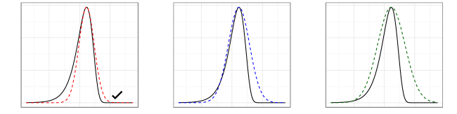
Figure 1: A "target" posterior density (solid line, same in all panels), and three scaled normal densities (dotted lines, increasing in covariance from left to right).

It is possible that $g(\theta)$ could under-sample values of $\theta$ in the tails of the posterior. However, if $M$ is sufficiently large, and $\Phi(\theta|y)\leq 1$ for all $M$ proposals, then it is unlikely that we would see $\Phi(\theta|y)>1$ in the rejection sampling phase of the algorithm. If that were to happen, we can stop, rescale, and try again. Any values of $\theta$ that we might miss would have such low posterior density that there would be little meaningful effect on inferences we might make from the output.

We believe that the potential cost from under-sampling the tails is dwarfed by our method’s relative computational advantage, we recognize that there may be some applications for which sampling extreme values of $\theta$ may be important. In that case, this may not be the best estimation method for those applications. Otherwise, there is nothing special about using the MVN for $g(\theta)$. It is straightforward to implement with manual adaptive selection of $s$. This is similar, in spirit, to the concept of tuning a Metropolis-Hastings algorithm. Heavier-tailed proposals, such as the multivariate-t distribution, can fail because of high kurtosis at the mode.

2.4 Comparison to Other Methods

2.4.1 Rejection Sampling

At first glance, our method looks quite similar to standard rejection sampling. With rejection sampling, one repeatedly samples both a threshold value from a standard uniform distribution ($p(u)=1$), and a proposal from $g(\theta)$ until $\pi(\theta|y)/g(\theta)\geq Ku$, where $K$ is a positive constant. This is different from our method, for which the threshold values are sampled from a posterior $p(u|y)$, and $K$ is specifically defined as the ratio of modal densities of the posterior to the proposal. The advantages that rejection sampling has over our approach is that the distribution of $u$ is exact, and that the proposal density does not have to dominate the target density for all values of $\theta$. However, for any model with more than a few dimensions, the critical ratio can be extremely small for even small deviations of $\theta$ away from the mode. Thus, the acceptance probabilities are virtually nil. In contrast, we accept a discrete approximation of $p(u|y)$ in exchange for higher acceptance probabilities.

2.4.2 Direct Sampling

[43] introduced and demonstrated the merits of a non-MCMC approach called Direct Sampling for conducting Bayesian inference. Like our method, Direct Sampling removes the need to concern oneself with issues like chain convergence and autocorrelation, and generates independent samples from a target posterior distribution in parallel. [43] also prove that the sample acceptance probabilities using Direct Sampling are better than those from standard rejection algorithms. Put simply, for many common Bayesian models, they demonstrate improvement over MCMC in terms of efficiency, resource demands and ease of implementation.

However, Direct Sampling suffers from some important shortcomings that limit its broad applicability. One is the failure to separate the specification of the prior from the specifics of the estimation algorithm. Another is an inability to generate accepted draws for even moderately sized problems; the largest number of parameters that Walker et al. consider is 10. Our method allows us to conduct full Bayesian inference on hierarchical models in high dimensions, with or without conjugacy, without MCMC.

Although we share some important features with Direct Sampling, our method differs in several respects. While Direct Sampling focuses on the shape of the data likelihood alone, we are concerned with the characteristics of the entire posterior density. Our method bypasses the need for Bernstein polynomial approximations, which are integral to the Direct Sampling algorithm. Finally, while Direct Sampling takes proposal draws from the prior (which may conflict with the data), our method samples proposals from a separate density that is ideally a good approximation to the target posterior density itself.

2.4.3 Markov chain Monte Carlo

We have already mentioned the key advantage of our method over traditional MCMC: generating independent samples that can be collected in parallel. We do not need to be concerned with issues like autocorrelation, convergence of estimation chains, and so forth. Without delving into a discussion of all possible variations and improvements to MCMC that have been proposed in the last few decades, there have been some attempts to parallelize MCMC that deserve some mention. For a deeper analysis, see [41].

It is possible to run multiple independent MCMC chains that start from different starting points. Once all of those chains have converged to the posterior distribution, we can estimate the posterior by combining samples from all of the chains. The numerical efficiency of that approximation should be higher than if we used only one chain, because there should be no correlation between samples collected in different chains. However, each chain still needs to converge to the posterior independently, and only after that convergence could we start collecting samples. If it takes a long time for one chain to converge, it will take at least that long for all chains to converge. Thus, the potential for parallelization is much greater for our method than for MCMC.

Another approach to parallelization is to exploit parallel processing power for individual steps in an algorithm. One example is a parallel implementation of a multivariate slice sampler (MSS), as in [42]. The benefits of parallelizing the MSS come from parallel evaluation of the target density at each of the vertices of the slice, and from more efficient use of resources to execute linear algebra operations (e.g, Cholesky decompositions). But the MSS itself remains a Markovian algorithm, and thus will still generate dependent draws. Using parallel technology to generate a single draw from a distribution is not the same as generating all of the required draws themselves in parallel. The sampling steps of our method can be run in their entirety in parallel.

Another attractive feature of our method is that the model is fully specified by the log posterior, and possibly its gradient and Hessian. The tools that we discuss in Section 4 are components of a reusable infrastructure. Only the function that returns the log posterior changes from model to model. This feature is unlike a blockwise Gibbs sampler, for which we need to derive and implement a set of conditional densities for each model. A small change in the model specification can require a substantial change in the sampling strategy. For example, a change to a prior might mean that the sampler is no longer conditionally conjugate. So while it might be possible to construct a highly efficient Gibbs sampler for a particular model (e.g., through blocking, data augmentation, or parameter transformation), there can be considerable upfront investment in doing so.

3 Examples

We now provide three examples of our method in action. In the first example, we simulate data from a basic, conditionally conjugate model, and compare the marginal posterior distributions that were generated by our method with those from a Gibbs sampler. The second example is a non-conjugate hierarchical model of store-level retail sales. In that example, we compare estimates from our method with those from Hamiltonian Monte Carlo (HMC), using the Stan software package [40]. For these first two examples, the MCMC methods are efficient, so it is likely that they generate good estimates of the true posterior densities. Thus, we can use those estimates as benchmarks against which we can assess the accuracy of our method. The third example is a more complicated model for which MCMC performs poorly. We use this example to not only assess the accuracy of our method (for those parameters for which we think the MCMC estimates are reasonable), but to illustrate some of the computational problems that are inherent in MCMC methods. In all of our examples, we implemented our method using the bayesGDS package [5] for R.

3.1 Simulated data, conditionally conjugate model

In our first example, we simulated $T=10$ observations for each of $N=1500$ heterogeneous units. Each observation for unit $i=1\mathellipsis N$ is a sample from a normal distribution, with mean $\theta_{i}$ and standard deviation $\sigma=2$. The $\theta_{i}$ are normally-distributed across the population, with mean $\mu=-1$ and standard deviation $\tau=3$. We place uniform priors on $\mu$, $\log\sigma$ and $\tau$. There are 1,503 parameters in this model.

This model allows for a conditionally conjugate Gibbs sampler; the steps are described in [23]. In this case, the Gibbs sampler is sufficiently fast and efficient, so we have confidence that it does indeed sample from the correct posterior distributions. The Gibbs sampler was run for 2,000 iterations, including a 1,000-iteration burn-in. The process took about five minutes to complete. We then collected 360 independent samples using our method, after estimating $q_{v}(v)$ with $M=70,000$ proposals, and applying a scaling factor on the inverse Hessian of 1.02. To get those 360 proposals, we needed 381,507 proposals. Using a single core of a 2014-vintage Mac Pro, this process would take about 23 minutes. However, each draw can be collected in parallel. It took about five minutes to collect all 360 samples when using 12 processing cores. The mean number of proposals for each posterior sample was 1,060 (an acceptance rate of .0009), but the median was only 29. Ten of the 360 samples required more than 10,000 proposals.

Figure 2 shows the quantiles of samples in the estimated marginal posterior densities of the population-level parameters $\mu$, $\tau^{2}$, and $\sigma^{2}$, as well as the log of the unnormalized posterior density. We can see that both methods generate effectively the same estimated posterior distributions.

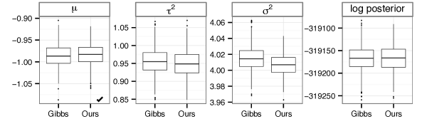
Figure 2: Quantiles of posterior densities from hierarchical model with conditional conjugacy, as estimated using our method, and with a Gibbs sampler.

3.2 Hierarchical model without conditional conjugacy

In the second example, we model weekly sales of sliced cheese in 88 retail stores. The data are available in the bayesm package for R [37], and were used in [4]. Under this model, mean sales for store $i$ in week $t$ has a gamma distribution with mean $\lambda_{it}$ and shape $r_{i}$. The mean is a log-linear function of price, and the percentage of “all category volume” on display in that week.

$$\log\lambda_{it}=\beta_{i1}+\beta_{i2}\log\text{PRICE}_{it}+\beta_{i3}\text{DISP}_{it}$$ (16)

The prior on each $r_{i}$ is a half-Cauchy distribution with a scale parameter of 5, and the prior on each $\beta_{i}$ is MVN with mean $\mu$ and covariance $\Omega$. The hyperparameters $\mu$ and $\Omega$ have weakly informative MVN and inverse Wishart priors, respectively. There are 361 parameters in this model.

This model does not allow for a conditionally conjugate Gibbs sampler. Instead, we use Hamiltonian Monte Carlo (HMC, [19, 31]), which uses the gradient of the log posterior to simulate a dynamic physical system. We selected HMC mainly because it is known to generate successive samples that are less serially correlated than draws that one might sample using other MCMC methods.

We implemented HMC using the Stan software package [40]. We ran 5 parallel chains for 800 iterations each, and discarding the first half of the draws. The chains appeared to display little autocorrelation, so we have confidence that the HMC samples form a good estimate of the true posterior distributions. We then estimated the model using our method with different numbers of proposal draws to estimate $q_{v}(v)$, and different scale factors on the covariance of the proposal density. In Figure 3, we compare the estimates densities for elements of $\mu$, the baseline and marginal effects on sales. We see that even with a relatively coarse estimate of $q_{v}(v)$, and an overly diffuse proposal density, our method generates estimates of the posterior densities that are not only comparable with each other, but also comparable those generated by Stan. The acceptance rates across different runs using our method was .0003. It took about 1.4 seconds to sample and evaluate a block of 1,000 proposals on a single processing core.

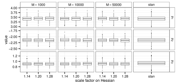
Figure 3: Estimated posterior densities of $\mu$ for the sliced cheese example.

3.3 Model with weakly identified parameters

Our third example concerns a non-conjugate heterogeneous hierarchical model, in which some parameters are only weakly identified. The data structure is described in [30]; we use the simulated data that are available in the bayesm package for R [37]. In this dataset, for each of 1,000 physicians, we observe weekly prescription counts for a single drug ($y_{it}$), weekly counts of sales visits from representatives of the drug manufacturer ($x_{it}$), and some time-invariant demographic information ($z_{i}$). Although one could model the purchase data as conditional on the sales visits, [30] argue that the rate of these contacts is determined endogenously, so that physicians who are expected to write more prescriptions, or who are more responsive to the sales visits, will receive visits more often.

In this model, $y_{it}$ is a random variable that follows a negative binomial distribution with shape $r$ and mean $\mu_{it}$, and $x_{it}$ is a Poisson-distributed random variable with mean $\eta_{i}$. The expected number of prescriptions per week depends in the number of sales visits, so we let $\log\mu_{it}=\beta_{i0}+\beta_{i1}x_{it}$, where $\beta_{i}$ is a vector of heterogeneous coefficients. We then model the contact rate so it depends on the physician-specific propensities to purchase, so $\log\eta_{i}=\gamma_{0}+\gamma_{1}\beta_{i0}+\gamma_{2}\beta_{i1}$. Define $z_{i}$ as a vector of four physician-specific demographics (including an intercept), and define $\Delta$ as a $2\times 4$ matrix of population-level coefficients. The mixing distribution for $\beta$ (i.e., the prior on each $\beta_{i}$), is MVN with mean $\Delta^{\prime}z_{i}$ and covariance $V$. We place weakly informative MVN priors on $\gamma$ and the rows of $\Delta$, an inverse Wishart prior on $V$, and a gamma prior on $r$. There are 2,015 distinct parameters to be estimated. This model differs slightly from the one in [30] only in that $\eta_{i}$ depends only on expected sales in the current period, and not the long-term trend. We made this change to make it easier to run the baseline MCMC algorithm.

As before, our baseline estimation algorithm is HMC, but instead of using Stan, we use the “double averaging” method to adaptively scale the step size [27], and we set the expected path length to 16. By implementing HMC ourselves, we can use the same computer code to compute the log posterior, and its gradient, that we use with our method. This allows the two methods to compete on a level playing field.

We ran four independent HMC chains for 700,000 iterations each, during a period of more than three weeks. Searching for the posterior mode is considered, in general, to be “good practice” for Bayesian inference, and especially with MCMC; see Step 1 of the “Recommended Strategy for Posterior Simulation” in Section 11.10 of [23]. Finding the mode of the log posterior is the first step of our method anyway, so we initialized one chain there, and the other three at randomly-selected starting values. Figure 4 is a trace plots of the log posterior density. The chains begin to approach each other only after about 500,000 iterations. The panels in Figure 5, are trace plots of the population-level parameters. Some parameter chains appear to have converged to each other, with little autocorrelation, but others seem to make no progress at all. Table 1, summarizes the effective sample sizes for estimates of the marginal posterior distributions of population-level parameters, using the final 100,000 samples of the HMC chains. Many of these parameters may require more than a million additional iterations to achieve an effective sample size large enough to make reasonable inferences.

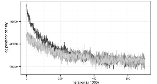
Figure 4: HMC trace plot of log posterior density for four chains. One chain was started at the mode, and the others started at random values. Every 500th iteration is plotted.

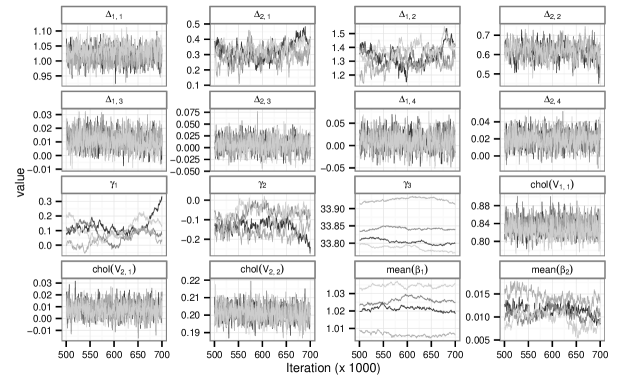
Figure 5: HMC trace plot for value of population-level parameters in hierarchical model example, starting at Iteration 500,000. Every 500th iteration is plotted.

	Chain						Chain
	1	2	3	4			1	2	3	4
$\Delta_{1,1}$	295	250	266	267		$\gamma_{1}$	3	4	6	2
$\Delta_{1,2}$	16	24	27	29		$\gamma_{2}$	10	33	22	22
$\Delta_{1,3}$	6	12	26	14		$\gamma_{3}$	3	15	3	3
$\Delta_{1,4}$	51	43	43	60		$\operatorname{Chol}(V)_{1,1}$	553	513	500	511
$\Delta_{2,1}$	4703	5933	5981	1444		$\operatorname{Chol}(V)_{2,1}$	7844	18761	13796	9852
$\Delta_{2,2}$	507	573	526	538		$\operatorname{Chol}(V)_{2,2}$	530	523	517	477
$\Delta_{2,3}$	407	445	400	407		mean($\beta_{1i}$)	6	5	12	12
$\Delta_{2,4}$	3708	4797	3680	4926		mean($\beta_{2i}$)	21	22	28	10

Table 1: Effective sample sizes for estimates of marginal posterior distributions of population-level parameters, using the final 100,000 samples of HMC chains.

The convergence problems are even worse when we consider that each of the 16 steps in the path length for iteration requires one evaluation for both the log posterior and its gradient. Using “reverse mode” automatic differentiation, which we discuss more in Section 4.1, the time to evaluate the gradient is about five times the time it takes to evaluate the log posterior, regardless of the number of variables [26]. Therefore, each HMC iteration requires resources that equate to 96 evaluations of the posterior. In other words, the computational cost of 700,000 HMC iterations is equivalent to more than 67 million evaluations of the log posterior. And this assumes that 700,000 iterations were sufficient to collect enough samples from the true posterior.

So how much more efficient is our sampling method? We estimated the marginal density $q_{v}(v)$ by taking $M=100,000$ proposal draws from an MVN distribution with the mean at the posterior mode $\theta^{*}$, and the covariance matrix equal the inverse of the Hessian at the mode, multiplied by a scaling factor of $s=1.3$. This value of $s$ is the smallest value for which $0\leq\Phi(\theta|y)\leq 1$ for all 100,000 samples from $g(\theta)$. We then collected 300 independent samples in parallel from the target posterior $\pi(\theta|y)$. The median number of proposals required for each posterior sample was just under 38,000, the total number of likelihood evaluations was about 16.5 million, and average acceptance rate was $1.8\times 10^{-5}$.

In absolute terms, the low acceptance rate appears to be unfavorable. However, the total run time is much lower than for MCMC. In our implementation (using a single core on a 2014-vintage Apple Mac Pro), the total time to compute the log posterior density of 1,000 proposal samples is about 8.7 seconds. The time to sample 1,000 proposals from an MVN distribution, and compute the MVN densities for each, is about .89 seconds. Therefore, to collect and evaluate 16.5 million proposal samples (to get 300 posterior draws) would take about 44 hours. But this is for a single processing core. Using all 12 cores on our Mac Pro, the sampling time is reduced to 220 minutes. We discuss the scalability of the component steps of the algorithm in Section 4.

Access to more processing nodes could reduce this time even further. It is the ability to collect posterior samples in parallel that gives our method its greatest advantage over MCMC methods. One could run multiple MCMC chains in parallel, but this involves waiting until all of the chains, individually, converge to the target posterior, before we could begin collecting samples for inference. Even then, there is no way to confirm that the chain has, in fact, converged.

We can draw inferences about the accuracy of our method by comparing the estimated marginal densities to those that we get from HMC. Note that the HMC estimates are accurate only if all of the chains converge to the target density, and we have a large-enough effective sample size. This condition clearly does not hold, but it is sufficiently close for the majority of the population-level parameters for us to use HMC samples as a baseline standard. Figure 6 is a comparison of the quantiles. For the elements of $\Delta$ and the Cholesky decomposition of $V$, our method’s estimated distributions are close to the HMC estimates. For other parameters, the convergence of the estimates is less clear. However, the parameters for which the densities are not aligned are the same parameters for which there is high autocorrelation, and little movement, in the HMC chains. Thus, we infer that our method compares with HMC well in terms of the marginal densities that it generates, with substantially computational effort.

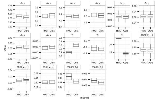
Figure 6: Estimated marginal distributions for population-level parameters using our method, and HMC.

4 Scalability and Sparsity

The ability for our method to generate independent samples in parallel already makes it an attractive alternative to MCMC. In this section, we present an argument in favor of our method’s scalability. Our criterion for scalability is that the cost of running the algorithm grows close to linearly in the number of households. Our analysis considers the fundamental computational tasks involved: computing the log posterior, its gradient and its Hessian; computing the Cholesky decomposition of the Hessian; and sampling from an MVN proposal distribution. We will show that scalability can be achieved because, under the conditional independence assumption, the Hessian of the log posterior is sparse, with a predictable sparsity pattern.

4.1 Computing Log Posteriors, Gradients and Hessians

Under the conditional independence assumption, the log posterior density is the sum of the logs of Equations 2 and 3, with a heterogeneous component

$$\sum_{i}^{N}\log f_{i}\left(y_{i}|\beta_{i},\alpha\right)+\log\pi_{i}(\beta_{i}|\alpha)$$ (17)

and a homogeneous component $\log\pi(\alpha)$. This homogeneous component is the hyperprior on the population-level parameters, so its computation does not depend on $N$, while each additional household adds another element to the summation in Equation 17. Therefore, computation of the log posterior grows linearly in $N$. In the subsequent text, let $k$ be the number of elements in each $\beta_{i}$ and let $p$ be the number of elements in $\alpha$. Using the notation from Section 2, $\theta$ is a vector that concatenates all of the $\beta_{i}$ together, along with $\alpha$.

There are two reasons why we might need to compute the gradient and Hessian of the log posterior, namely to use in a derivative-based optimization algorithm to find the posterior mode, and for estimating the precision matrix of an MVN proposal distribution. Ideally, we would derive the gradient and Hessian analytically, and write code to estimate it efficiently. For complicated models, the required effort for coding analytic gradients may not be worthwhile. An alternative would be numerical approximation through finite differencing. The fastest, yet least accurate, method for finite differencing for gradients, using either forward or backward differences, requires $Nk+p+1$ evaluations of the log posterior. Since the computational cost of the log posterior also grows linearly with $N$, computing the gradient this way will grow quadratically in $N$. The cost of estimating a Hessian using finite differencing grow even faster in $N$. Also, if the Hessian is estimated by taking finite differences of gradients, and those gradients themselves were finite-differences, the accumulated numerical error can be so large that the Hessian estimates are useless.

Instead, we can turn to automatic differentiation (AD, also sometimes known as algorithmic differentiation). A detailed explanation of AD is beyond the scope of this paper, so we refer the reader to [26], or Section 8.2 in [33]. Put simply, AD treats a function as a composite of subfunctions, and computes derivatives by repeatedly applying the chain rule. In practical terms, AD involves coding the log posterior using a specialized numerical library that keeps track of the derivatives of these subfunctions. When we compile the function that computes the log posterior, the AD library will “automatically” generate additional functions that return the gradient, the Hessian, and even higher-order derivatives.

The remarkable feature of AD is that computing the gradient of a scalar-valued function takes no more than five times as long as computing the log posterior, regardless of the number of parameters [26, p. xii]. If the cost of the log posterior grows linearly in $N$, so will the cost of the gradient.

In most statistical software packages, like R, the default storage mode for any matrix is in a “dense” format; each element in the matrix is stored explicitly, regardless of the value. For a model with $n$ variables, this matrix consists of $n^{2}$ numbers, each consuming eight bytes of memory at double precision. If we have a dataset in which $N=10000$, $k=5$ and $p$ is relatively small, the Hessian for this model with $50,000+p$ variables will consume more than 20GB of RAM. Furthermore, the computational effort for matrix-vector multiplication is quadratic in the number of columns, and matrix-matrix multiplication is cubic. To the extent that either of these operations is used in the mode-finding or sampling steps, the computational effort will grow much faster than the size of the dataset. Since multiplying a triangular matrix is roughly one-sixth as expensive as multiplying a full matrix, we could gain some efficiency by working with the Cholesky decomposition of the Hessian instead. However, the complexity of the Cholesky decomposition algorithm itself will still be cubic in $N$ [25, Ch. 1].

For our purposes, the source of scalability is in the sparsity of the Hessian. If the vast majority of elements in a matrix are zero, we do not need to store them explicitly. Instead, we need to store only the non-zero values, the row numbers of those values, and the index of the values that begin each column. Under the conditional independence assumption, the cross-partial derivatives between heterogeneous parameters across households are all zero. Thus, the Hessian becomes sparser as the size of the dataset increases.

To illustrate, suppose we have a hierarchical model with six households, two heterogeneous parameters per household, and two population-level parameters, for a total of 14 parameters. Figure 7 is a schematic of the sparsity structure of the Hessian; the vertical lines are the non-zero elements, and the dots are the zeros. There are 196 elements in this matrix, but only 169 are non-zero, and only 76 values are unique. Although the savings in RAM is modest in this illustration, the efficiencies are much greater when we add more households. If we had 1,000 households, with $k=3$ and $p=9$, there would be 3009 parameters, and more than nine million elements in the Hessian, yet no more than 63,000 are non-zero, of which about 34,500 are unique. As we add households, the number of non-zero elements of the Hessian grows only linearly in $N$.

 [1,] | | . . . . . . . . . . | |  [2,] | | . . . . . . . . . . | |  [3,] . . | | . . . . . . . . | |  [4,] . . | | . . . . . . . . | |  [5,] . . . . | | . . . . . . | |  [6,] . . . . | | . . . . . . | |  [7,] . . . . . . | | . . . . | |  [8,] . . . . . . | | . . . . | |  [9,] . . . . . . . . | | . . | | [10,] . . . . . . . . | | . . | | [11,] . . . . . . . . . . | | | | [12,] . . . . . . . . . . | | | | [13,] | | | | | | | | | | | | | | [14,] | | | | | | | | | | | | | |

Figure 7: Example of sparsity pattern under conditional independence.

The cost of estimating a dense Hessian using AD grows linearly with the number of variables [26]. When the Hessian is sparse, with a pattern similar to Figure 7, we can estimate the Hessian so that the cost is only a multiple of the cost of computing the log posterior. We achieve this by using a graph coloring algorithm to partition the variables into a small number of groups (or “colors” in the graph theory literature), such that a small change in the variable in one group does not affect the partial derivative of any other variable in the same group. This means we could perturb all of the variables in the same group at the same time, recompute the gradient, and after doing that for all groups, still be able to recover an estimate of the Hessian. Thus, the computational cost for computing the Hessian grows with the number of groups, not the number of parameters. Because the household-level parameters are conditionally independent, we do not need to add groups as we add households. For the Hessian sparsity pattern in Figure 7, we need only four groups: one for each of the heterogeneous parameters across all of the households, and one for each of the two population-level parameters. In the upcoming binary choice example in Section 4.4, for which $k=3$, there are $\frac{1}{2}\left(k^{2}+5k\right)=12$ groups, no matter how many households we have in the dataset.

[17] introduce the idea of reducing the number of evaluations to estimate sparse Jacobians. [34] describe how to partition variables into appropriate groups, and how to recover Hessian information through back-substitution. [13] show that the task of grouping the variables amounts to a classic graph-coloring problem. Most AD software applies this general principle to computing sparse Hessians. Alternatively, R users can use the sparseHessianFD package [6] to efficiently estimate sparse Hessians through finite differences of the gradient, as long as the sparsity pattern is known in advance, and as long as the gradient was not itself estimated through finite differencing. This package is an interface to the algorithms in [15] and [14].

4.2 Finding the posterior mode

For simple models and small datasets, standard default algorithms (like the optim function in R) are sufficient for finding posterior modes and estimating Hessians. For larger problems, one should choose optimization tools more thoughtfully. For example, many of the R optimization algorithms default to finite differencing of gradients when a gradient function is not provided explicitly. Even if the user can provide the gradient, many algorithms will store a Hessian, or an approximation to it, densely. Neither feature is attractive when the number of households is large.

For this section, let’s assume that the log posterior is twice-differentiable and unimodal. There are two approaches that one can take. The first is to use a “limited memory” optimization algorithm that approximates the curvature of the log posterior over successive iterations. Several algorithms of this kind are described in [33], and are available for many technical computing platforms. Once the algorithm finds the posterior mode, there remains the need to compute the Hessian exactly.

The second approach is to run a quasi-Newton algorithm, and compute the Hessian at each iteration explicitly, but store the Hessian in a sparse format. The trustOptim package for R [8] implements a trust region algorithm that exploits the sparsity of the Hessian. The user can supply a Hessian that is derived analytically, computed using AD, or estimated numerically using sparseHessianFD. Since memory requirements and matrix computation costs will grow only linearly in $N$, finding the posterior mode becomes feasible for large problems, compared to similar algorithms that ignore sparsity.

We should note that we cannot predict the time to convergence for general problems. Log posteriors with ridges or plateaus, or that require extensive computation themselves, may still take a long time to find the local optimum. Whether any mode-finding algorithm is “fast enough” depends on the specific application. However, if one optimization algorithm has difficulty finding a mode, another algorithm may do better.

4.3 Sampling from an MVN distribution

Once we find the posterior mode, and the Hessian at the mode, generating proposal samples from an MVN($\theta^{*},sH^{-1}$) distribution is straightforward. Let $\frac{1}{s}H=\Lambda\Lambda^{\prime}$ represent the Cholesky decomposition of the precision of the proposal, and let $z$ be a vector of $Nk+p$ samples from a standard normal distribution. To sample $\theta$ from an MVN, solve the triangular linear system $\Lambda^{\prime}\theta=x$, and then add $\theta^{*}$. Since $E(z)=0$, $E(\theta)=\theta^{*}$, and since $E(zz^{\prime})=I$, $\operatorname{cov}(\theta)=\Lambda^{\prime-1}\Lambda^{-1}=(\Lambda\Lambda^{\prime})^{-1}=sH^{-1}$.

Because $\Lambda$ is sparse, the costs of both solving the triangular system, and the premultiplication, grow linearly with the number of nonzero elements, which itself grows linearly in $N$ [18]. If $\Lambda$ were dense, then the cost of solving the triangular system would grow quadratically in $N$. Furthermore, computing the MVN density would involve premultiplying $z$ by a triangular matrix, whose cost is cubic in $N$ [25].

Computation of the Cholesky decomposition can also benefit from the sparsity of the Hessian. If $H$ were dense $Nk+p$ square, symmetric matrix, then, holding $k$ and $p$ constant, the complexity order of the Cholesky decomposition is $N^{3}$ [25]. There are a number of different algorithms that one can use for decomposing sparse Hessians [18]. The typical strategy is to first permute the rows and columns of $H$ to minimize the number of nonzero elements in $\Lambda$, and then compute the sparsity pattern. This part can be done just once. With the sparsity pattern in hand, the next step is to compute those nonzero elements in $\Lambda$. The time for this step grows with the sum of the squares of the number of nonzero elements in each column of $\Lambda$ [18]. Because each additional household adds $k$ columns to $\Lambda$, with an average of $p+\frac{1}{2}(k+1)$ nonzero elements per column, we can compute the sparse Cholesky decomposition in time that is linear in $N$. Software for sparse Cholesky decompositions is widely available.

4.4 Scalability Test

Next, we provide some empirical evidence of scalability through a simulation study. For a hypothetical dataset with $N$ households, let $y_{i}$ be the number of times household $i$ visits a store during a $T$ week period. The probability of a visit in a single week is $p_{i}$, where $\operatorname{logit}p_{i}=\beta_{i}^{\prime}x_{i}$, and $x_{i}$ is a vector of $k$ covariates. The distribution of $\beta_{i}$ across the population is MVN with mean $\bar{\beta}$ and covariance $\Sigma$. In all conditions of the test, we set $k=3$ and $T=52$, and vary the number of households by setting $N$ to one of 10 discrete values from 500 to 50,000. The “true” values of $\bar{\beta}$ are -10, 0 and 10, and the “true” $\Sigma$ is $0.1I$. We place weakly informative priors on both $\bar{\beta}$ and $\Sigma$.

In Figure 8, we plot the average time, across 100 replications, to compute the log posterior, the gradient, and the Hessian. As expected, each of these computations grows linearly in $N$. In Figure 9, we plot average times for the steps involved in sampling from an MVN: adding a vector to columns of a dense matrix, computing a sparse Cholesky decomposition, multiplying a sparse triangular matrix by a dense matrix, sampling standard normal random variates, and solving a sparse triangular linear system. Again, we see that the time for all of these steps is linear in $N$.

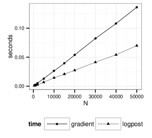
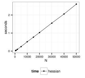
Figure 8: Average computation time for 100 evaluations of log posterior, gradient and Hessian.

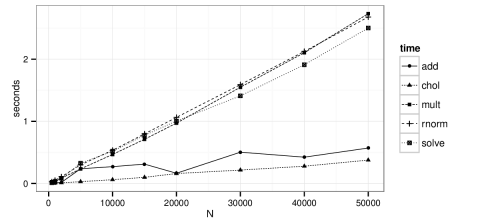
Figure 9: Computation time, averaged over 100 replications, for adding a vector to matrix columns (add); a sparse Cholesky decomposition (chol); multiplying a sparse triangular matrix by a dense matrix (mult); sampling standard normal random variates (rnorm); and solving a sparse triangular linear system (solve)

Table 2 summarizes the acceptance rates and scale factors when generating 50 samples from the posterior for different values of $N$. Although there is a weak trend of increasing acceptance rates with $N$,we cannot say with any certainty that acceptance rates will always be either larger or smaller for larger datasets. The acceptance rate could be influenced by using different scale factors on the Hessian for the MVN proposal density. However, we expect higher acceptance rates as the target posterior density approaches an MVN asymptotically. Since none of the steps in the algorithm grows faster than linearly in $N$, we are confident in the scalability of the overall algorithm.

N	500	1,000	2,000	5,000	10,000	15,000	20,000	30,000	40,000	50,000
scale factor	1.22	1.16	1.10	1.08	1.04	1.03	1.03	1.03	1.03	1.02
acc. rate ($\times 10^{-5}$)	2.1	1.5	2.6	0.7	2.9	2.6	3.6	3.9	2.7	3.3

Table 2: Acceptance rates for binary choice simulation. For each condition, $k=3$, so there are six population-level parameters and $3N$ heterogeneous parameters.

5 Estimating Marginal Likelihoods

Now, we turn to another advantage of our method: the ability to generate accurate estimates of the marginal likelihood of the data with little additional computation. A number of researchers have proposed methods to approximate the marginal likelihood, $\mathcal{L}(y)$ from MCMC output [22, 32, 12, 36], but none has achieved universal acceptance as being consistent, stable and easy to compute. In fact, [28] demonstrated that methods that depend solely on samples from the posterior density could suffer from a “pseudo-bias,” and he proposes an importance-sampling method to correct for it. This pseudo-bias arises because the convex hull of MCMC samples defines only a subset of the posterior support, while $\mathcal{L}(y)$ is defined as an integral of the data likelihood over the prior distribution. [28] demonstrates that his method dominates other popular methods, although with substantial computational effort. Thus, the estimation of the marginal likelihood remains a difficult problem in MCMC-based Bayesian statistics.

We estimate the marginal likelihood using quantities that we already collect during the course of the estimation procedure. Recall that $q(u)$ is the probability that, given a threshold value $u$, a proposal from $g(\theta)$ is accepted as a sample from $\pi(\theta|y)$. Therefore, after substituting in Equation 8, we can express the expected marginal acceptance probability for any one posterior sample as

$$\gamma =\int_{0}^{1}q(u)p(u|y)~{}du=\frac{c_{1}}{c_{2}\mathcal{L}(y)}\int_{0}^{1}q^{2}(u)~{}du$$ (18)

Applying a change of variables so $v=-\log u$, and then rearranging terms,

$$\mathcal{L}(y) =-\frac{c_{1}}{c_{2}\gamma}\int_{0}^{\infty}q^{2}(v)\exp(-v)~{}dv.$$ (19)

The values for $c_{1}$ and $c_{2}$ are immediately available from the algorithm. A reasonable estimator of $\gamma$ is $\hat{\gamma}$, the inverse of the mean of the observed average number of proposals per accepted sample. What remains is estimating the integral in Equation 19, for which we use the same proposal draws that we already collected for estimating $\widehat{q}_{v}(v)$. The empirical CDF of these draws is discrete, so we can partition the support of $q_{v}(v)$ at $v_{1}\mathellipsis v_{M}$. Also, since $\widehat{q}_{v}(v)$ is the proportion of proposal draws less than $v$, we have $q_{v}(v_{i})=i/M$. Therefore,

$$\int_{0}^{\infty}q^{2}(v)\exp(-v)dv \approx\sum_{i=1}^{M}\int_{v_{i}}^{v_{i+1}}\left(\frac{i}{M}\right)^{2}\exp(-v_{i})dv$$ (20)

$$=\frac{1}{M^{2}}\sum_{i=1}^{M}i^{2}\left[\exp(-v_{i})-\exp(-v_{i+1})\right]$$ (21)

$$=\frac{1}{M^{2}}\sum_{i=1}^{M}\left(2i-1\right)\exp(-v_{i})$$ (22)

Putting all of this together, we can estimate the marginal likelihood as

$$\mathcal{L}(y) \approx\frac{c_{1}}{M^{2}c_{2}\hat{\gamma}}\sum_{i=1}^{M}(2i-1)\exp(-v_{i})$$ (23)

As a demonstration of the accuracy of this estimator, we use the same linear regression example that [28] uses.

$$y_{it} \sim N(x_{i}^{\prime}\beta,\sigma^{2}),~{}i=1\mathellipsis n,t=1\mathellipsis T$$ (24)

$$\beta|\sigma \sim N(\beta_{0},\sigma^{2}V_{0})\qquad\sigma^{2}\sim IG(r,\alpha)$$ (25)

For this model, $\mathcal{L}(y)$ is a multivariate-t density (MVT), which we can compute analytically. This allows us to compare the estimates of $\mathcal{L}(y)$ with the “truth.” To do this, we conducted a simulation study for simulated datasets of different numbers of observations $n\in\{200,2000\}$ and numbers of covariates $k\in\{5,25,100\}$. For each $n,k$ pair, we simulated 25 datasets. For each dataset, each vector $x_{i}$ includes an intercept and $k$ iid samples from a standard normal density. Thus, there are $k+2$ parameters, corresponding to the elements of $\beta$, plus $\sigma$. The true intercept term is 5, and the remaining true $\beta$ parameters are linearly spaced from $-5$ to $5$. In all cases, there are $T=25$ observations per unit. Hyperpriors are set as $r=2$, $\alpha=1$, $\beta_{0}$ as a zero vector and $V_{0}=0.2\cdot I_{k}$.

For each dataset, we collected 250 samples from the posterior density, with different numbers of proposal draws ($M=1,000\text{ or }10,000$), and different scale factors ($s=0.5,0.6,0.7,\text{ or }0.8$) on the Hessian ($-sH$ is the precision matrix of the MVN proposal density, and lower scale factors generate more diffuse proposals). We excluded the $s=0.8$, $n=200$ case because the proposal density was not sufficiently diffuse to ensure that $\Phi(\theta|y)$ was between 0 and 1 across the $M$ proposal draws.

Table 3 presents the true log marginal likelihood (MVT), along with estimates using our method, the importance sampling method in Lenk (2009), and the harmonic mean estimator [32]. We also included the mean acceptance probabilities, and the standard deviations of the various estimates across the simulated datasets. We can see that our estimates for the log marginal likelihood are remarkably close to the MVT densities, and are robust when we use different scale factors. Accuracy appears to be better for larger datasets than smaller ones, while improving the approximation of $p(u|y)$ by increasing the number of proposal draws offers negligible improvement. Note that the performance of our method is comparable to that of Lenk, but is much better than the harmonic mean estimator. Our method is similar to Lenk’s in that it computes the probability that a proposal draw falls within the support of the posterior density. However, the inputs to the estimator of the marginal likelihood are intrinsically generated as the algorithm progresses. In contrast, the Lenk estimator requires an additional importance sampling run after the MCMC draws are collected.

				MVT		Ours		Lenk		HME		Mean
k	n	M	scale	mean	sd	mean	sd	mean	sd	mean	sd	Acc %
5	200	1000	0.5	-309	6.6	-309	6.6	-311	6.8	-287	7.1	22.1
5	200	1000	0.6	-309	6.6	-309	6.7	-310	6.9	-287	6.9	40.5
5	200	1000	0.7	-309	6.6	-309	6.7	-310	6.5	-287	6.3	57.1
5	200	10000	0.5	-309	6.6	-309	6.6	-311	6.7	-287	6.7	24.0
5	200	10000	0.6	-309	6.6	-309	6.6	-310	7.5	-287	6.8	40.9
5	200	10000	0.7	-309	6.6	-309	6.7	-310	7.0	-287	7.1	55.2
5	2000	1000	0.5	-2866	46.2	-2865	46.3	-2868	46.2	-2836	46.2	22.1
5	2000	1000	0.6	-2866	46.2	-2866	46.2	-2868	45.7	-2836	45.5	37.8
5	2000	1000	0.7	-2866	46.2	-2866	46.3	-2867	45.9	-2836	45.9	49.6
5	2000	1000	0.8	-2866	46.2	-2866	46.2	-2867	46.3	-2835	46.3	64.6
5	2000	10000	0.5	-2866	46.2	-2866	46.4	-2867	46.7	-2836	46.9	25.3
5	2000	10000	0.6	-2866	46.2	-2866	46.2	-2867	45.8	-2836	46.3	36.3
5	2000	10000	0.7	-2866	46.2	-2866	46.4	-2867	46.0	-2836	46.3	51.4
5	2000	10000	0.8	-2866	46.2	-2866	46.2	-2867	46.5	-2835	46.3	72.0
25	200	1000	0.5	-387	8.1	-385	8.2	-391	7.6	-292	8.5	2.8
25	200	1000	0.6	-387	8.1	-386	8.1	-390	9.5	-292	8.8	8.1
25	200	1000	0.7	-387	8.1	-386	8.3	-390	8.0	-292	8.8	16.2
25	200	10000	0.5	-387	8.1	-385	8.5	-390	8.2	-292	8.4	1.7
25	200	10000	0.6	-387	8.1	-385	8.2	-390	8.9	-292	8.8	6.2
25	200	10000	0.7	-387	8.1	-386	8.2	-390	8.7	-292	9.1	20.0
25	2000	1000	0.5	-2990	28.7	-2989	28.8	-2994	28.3	-2865	28.8	2.7
25	2000	1000	0.6	-2990	28.7	-2989	28.7	-2993	28.4	-2864	29.0	4.6
25	2000	1000	0.7	-2990	28.7	-2989	28.9	-2991	30.0	-2864	29.5	15.4
25	2000	1000	0.8	-2990	28.7	-2990	28.7	-2992	29.6	-2864	29.4	43.1
25	2000	10000	0.5	-2990	28.7	-2988	29.2	-2992	28.5	-2864	28.9	.8
25	2000	10000	0.6	-2990	28.7	-2989	29.1	-2993	29.4	-2864	28.9	3.7
25	2000	10000	0.7	-2990	28.7	-2990	29.0	-2993	28.9	-2864	28.9	17.1
25	2000	10000	0.8	-2990	28.7	-2990	28.6	-2993	28.2	-2865	28.2	43.3
100	200	1000	0.5	-660	6.7	-661	6.5	-683	8.8	-292	9.2	.3
100	200	1000	0.6	-660	6.7	-660	6.6	-678	8.5	-286	9.0	.3
100	200	1000	0.7	-660	6.7	-659	7.1	-673	7.8	-282	8.0	.4
100	200	10000	0.5	-660	6.7	-659	6.9	-682	9.1	-288	10.4	.1
100	200	10000	0.6	-660	6.7	-660	5.7	-678	8.8	-286	8.9	.1
100	200	10000	0.7	-660	6.7	-658	6.7	-674	7.3	-282	8.4	.1
100	2000	1000	0.5	-3364	24.4	-3364	24.8	-3370	27.5	-2871	27.1	.3
100	2000	1000	0.6	-3364	24.4	-3362	24.6	-3369	24.3	-2868	25.3	.6
100	2000	1000	0.7	-3364	24.4	-3361	23.9	-3371	25.6	-2870	25.4	1.1
100	2000	1000	0.8	-3364	24.4	-3362	23.9	-3370	26.0	-2868	26.1	3.2
100	2000	10000	0.5	-3364	24.4	-3362	24.0	-3372	25.3	-2870	25.2	.1
100	2000	10000	0.6	-3364	24.4	-3360	24.9	-3368	25.3	-2867	25.4	.1
100	2000	10000	0.7	-3364	24.4	-3360	24.6	-3370	25.5	-2869	25.5	.4
100	2000	10000	0.8	-3364	24.4	-3362	24.5	-3367	24.3	-2867	24.4	3.0

Table 3: Results of simulation study for effectiveness of estimator for log marginal likelihood.

6 Discussion of practical considerations and limitations

To those who have spent long work hours dealing with MCMC convergence and efficiency issues, the utility of an alternative algorithm is appealing. Ours allows for sampling from a posterior density in parallel, without having to worry about whether an MCMC estimation chain has converged. If heterogeneous units (like households) are conditionally independent, then the sparsity of the Hessian of the log posterior lets us construct a sampling algorithm whose complexity grows only linearly in the number of units. This method makes Bayesian inference more attractive to practitioners who might otherwise be put off by the inefficiencies of MCMC.

This is not to say that our method is guaranteed to generate perfect samples from the target posterior distribution. One area of potential concern is that the empirical distribution $\widehat{q}_{v}(v)$ is only a discrete approximation to $q_{v}(v)$. That discretization could introduce some error into the estimate of the posterior density. This error can be reduced by increasing $M$ (the number of proposal draws that we use to compute $\widehat{q}_{v}(v)$ ), at the expense of costlier computation of $\widehat{q}_{v}(v)$ and, possibly, lower acceptance rates. In our experience, and consistent with Figure 3, we have not found this to be a problem, but some applications for which this may be an issue might exist.

Like many other methods that collect random samples from posterior distributions, its efficiency depends in part on a prudent selection of the proposal density $g(\theta)$. For the examples in this paper, we use a MVN density that is centered at the posterior mode with a covariance matrix that is proportional to the inverse of the Hessian at the mode. One might then wonder if there is an optimal way to determine just how “scaled out” the proposal covariance needs to be. At this time, we think that manual search is the best alternative. If we start with a small $M$ (say, 100 draws), and find that $\Phi(\theta|y)>1$ for any of the $M$ proposals, we have learned that the proposal density is not valid, with little computational or real-time cost. We can then re-scale the proposal until $\Phi(\theta|y)<1$, and then gradually increase $M$ until we get a good approximation to $p(u)$. This is no different, in principle, than the tuning step in a Metropolis-Hasting algorithm. However, our method has the advantage that we can make these adjustments before the posterior sampling phase begins. In contrast, with adaptive MCMC methods an improperly tuned sampler might not be apparent until the chain has run for a substantial period of time. Also, even if an acceptance rate appears to be low, we can still collect draws in parallel, so the “clock time” remains much less than the time we spend trying to optimize selection of the proposal.

There are many popular models, such as multinomial probit, for which the likelihood of the observed data is not available in closed form. When direct numerical approximations to these likelihoods (e.g., Monte Carlo integration) are not tractable, MCMC with data augmentation is a possible alternative. Recent advances in parallelization using graphical processing units (GPUs) might make numerical estimation of integrals more practical than it was even 10 years ago [41]. If so, then our method could be a viable, efficient alternative to data augmentation in these kinds of models. Multiple imputation of missing data could suffer from the same kinds of problems, since a latent parameter, introduced for the data augmentation step, is only weakly identified on its own. If the number of missing data points is small, one could treat the representation of the missing data points as if they were parameters. But the implications of this require additional research.

Another opportunity for further research involves the case of multimodal posteriors. Our method does require finding the global posterior mode, and all the models discussed in this paper have unimodal posterior distributions. When the posterior is multimodal, one might instead use a mixture of normals as the proposal distribution. The idea is to not only find the global mode, but any local ones as well, and center each mixture component at each of those local modes. The algorithm itself would remain unchanged, as long as the global posterior mode matches the global proposal mode.

We recognize that finding all of the local modes could be a hard problem, and there is no guarantee that any optimization algorithm will find all local extrema in a reasonable amount of time. In practical terms, MCMC, offers no such guarantees either. Even if the log posterior density is unimodal, one should take care that the mode-finding optimizer does not stop until reaching the optimum. For R, trustOptim [8] is one such package, in that its stopping rule depends on the norm of the gradient being sufficiently close to zero.

There are a number of packages for the R statistical programming language that can help with implementation of our method. The bayesGDS package [5] includes functions to run the rejection sampling phase (lines 20-36 in Algorithm 1). This package also includes a function that estimates the log marginal likelihood from the output of the algorithm. If the proposal distribution is MVN, and either the covariance or precision matrix is sparse, then one can use the sparseMVN [7] package to sample from the MVN by taking advantage of that sparsity. The sparseHessianFD [6] package estimates a sparse Hessian by taking finite differences of gradients of the function, as long as the user can supply the sparsity pattern (which should be the case under conditional independence). Finally, the trustOptim package [8] is a nonlinear optimization package that uses a sparse Hessian to include curvature information in the algorithm.

References

- [1] Greg M Allenby, Eric T Bradlow, Edward I George, John Liechty and Robert E McCulloch “Perspectives on Bayesian Methods and Big Data” In Customer Needs and Solutions 1, 2014, pp. 169–175 DOI: 10.1007/s40547-014-0017-9
- [2] Douglas Bates and Dirk Eddelbuettel “Fast and Elegant Numerical Linear Algebra Using the RcppEigen Package” In Journal of Statistical Software 52.5, 2013, pp. 1–24
- [3] B. M. Bell “CppAD: a package for C++ algorithmic differentiation”, 2013 Computational Infrastructure for Operations Research URL: www.coin-or.org/CppAD
- [4] Peter Boatwright, Robert McCulloch and Peter Rossi “Account-Level Modeling for Trade Promotion: An Application of a Constrained Parameter Hierarchical Model” In Journal of the American Statistical Association 94.448, 1999, pp. 1063–1073
- [5] Michael Braun “bayesGDS: an R package for generalized direct sampling” R package version 0.6.0, 2013 URL: cran.r-package.org/web/packages/bayesGDS
- [6] Michael Braun “sparseHessianFD: An R package for estimating sparse Hessians” R package version 0.1.1, 2013 URL: cran.r-project.org/web/packages/sparseHessianFD
- [7] Michael Braun “sparseMVN: an R package for MVN sampling with sparse covariance and precision matrices.” R package version 0.1.0, 2013 URL: cran.r-project.org/web/packages/sparseMVN
- [8] Michael Braun “trustOptim: An R Package for Trust Region Optimization with Sparse Hessians” In Journal of Statistical Software 60.4, 2014, pp. 1–16 URL: http://www.jstatsoft.org/v60/i04/
- [9] “Handbook of Markov Chain Monte Carlo” Boca Raton, Fla.: ChapmanHall/CRC, 2010
- [10] Bradley P Carlin and Thomas A Louis “Bayes and Empirical Bayes Methods for Data Analysis” Boca Raton, Fla.: ChapmanHall/CRC, 2000
- [11] Ming-Hui Chen, Qi-Man Shao and Joseph G Ibrahim “Monte Carlo Methods in Bayesian Computation” New York: Springer, 2000
- [12] Siddhartha Chib “Marginal Likelihood from the Gibbs Output” In Journal of the American Statistical Association 90.432, 1995, pp. 1313–1321
- [13] Thomas F Coleman and Jorge J Moré “Estimation of Sparse Jacobian Matrices and Graph Coloring Problems” In SIAM Journal on Numerical Analysis 20.1, 1983, pp. 187–209
- [14] Thomas F Coleman, Burton S Garbow and Jorge J Moré “Algorithm 636: Fortran Subroutines for Estimating Sparse Hessian Matrices” In ACM Transactions on Mathematical Software 11.4, 1985, pp. 378
- [15] Thomas F Coleman, Burton S Garbow and Jorge J Moré “Software for Estimating Sparse Hessian Matrices” In ACM Transactions on Mathematical Software 11.4, 1985, pp. 363–377
- [16] Thomas F Coleman and Arun Verma “ADMIT-1: Automatic Differentiation and MATLAB Interface Toolbox” In ACM Transactions on Mathematical Software 26.1, 2000, pp. 150–175
- [17] A R Curtis, M J D Powell and J K Reid “On the Estimation of Sparse Jacobian Matrices” In Journal of the Institute of Mathematics and its Applications 13, 1974, pp. 117–119
- [18] Timothy A Davis “Direct Methods for Sparse Linear Systmes” Philadelphia: Society for IndustrialApplied Mathematics, 2006
- [19] Simon Duane, A D Kennedy, Brian J Pendleton and Duncan Roweth “Hybrid Monte Carlo” In Physics Letters B 195.2, 1987, pp. 216–222
- [20] Dirk Eddelbuettel and Romain François “Rcpp: Seamless R and C++ Integration” In Journal of Statistical Software 40.8, 2011, pp. 1–18
- [21] Alan E Gelfand and Adrian F M Smith “Sampling-Based Approaches to Calculating Marginal Densities” In Journal of the American Statistical Association 85.410, 1990, pp. 398–409
- [22] Alan E Gelfand and Dipak K. Dey “Bayesian Model Choice: Asymptotics and Exact Calculations” In Journal of the Royal Statistical Society, Series B 56.3, 1994, pp. 501–514
- [23] Andrew Gelman, John B Carlin, Hal S Stern and Donald B Rubin “Bayesian Data Analysis” Boca Raton, Fla.: ChapmanHall, 2003
- [24] Mark Girolami and Ben Calderhead “Riemann Manifold Langevin and Hamiltonian Monte Carlo” In Journal of the Royal Statistical Society, Series B 73, 2011, pp. 1–37
- [25] Gene H Golub and Charles F Van Loan “Matrix Computations” Johns Hopkins University Press, 1996
- [26] Andreas Griewank and Andrea Walther “Evaluating Derivatives: Principles and Techniques of Algorithmic Differentiation” Philadelphia: Society for IndustrialApplied Mathematics, 2008
- [27] Matthew D Hoffman and Andrew Gelman “The No-U-Turn Sampler: Adaptively Setting Path Lengths in Hamiltonian Monte Carlo” In Journal of Machine Learning Research 15, 2014, pp. 1593–1623
- [28] Peter Lenk “Simulation Pseudo-Bias Correction to the Harmonic Mean Estimator of Integrated Likelihoods” In Journal of Computational and Graphical Statistics 18.4, 2009, pp. 941–960
- [29] John D C Little “Models and Managers: The Concept of a Decision Calculus” In Management Science 16.8, 1970, pp. B466–B485
- [30] Puneet Manchanda, Peter E Rossi and Pradeep K Chintagunta “Response Modeling with Nonrandom Marketing-Mix Variable” In Journal of Marketing Research 41.4, 2004, pp. 467–478
- [31] Radford M Neal “MCMC Using Hamiltonian Dynamics” In Handbook of Markov Chain Monte Carlo Boca Raton, Fla.: CRC Press, 2011, pp. 113–162
- [32] Michael A Newton and Adrian E Raftery “Approximate Bayesian Inference with the Weighted Likelihood Bootstrap” In Journal of the Royal Statistical Society, Series B 56.1, 1994, pp. 3–48
- [33] Jorge Nocedal and Stephen J Wright “Numerical Optimization” Springer-Verlag, 2006
- [34] M J D Powell and Ph. L. Toint “On the Estimation of Sparse Hessian Matrices” In SIAM Journal on Numerical Analysis 16.6, 1979, pp. 1060–1074
- [35] R Development Core Team “R: A Language and Environment for Statistical Computing”, 2014 R Foundation for Statistical Computing
- [36] Adrian E Raftery, Michael A Newton, Jaya M Satagopan and Pavel N Krivitsky “Estimating the Integrated Likelihood via Posterior Simulation Using the Harmonic Mean Identity” In Bayesian Statistics 8 Proceedings, 2007, pp. 1–45
- [37] Peter Rossi “bayesm: Bayesian Inference for Marketing/Micro-econometrics” R package version 2.2-5, 2012 URL: cran.r-project.org/web/packages/bayesm
- [38] Peter E Rossi and Greg M Allenby “Bayesian Statistics and Marketing” In Marketing Science 22.3, 2003, pp. 304–328
- [39] Peter E Rossi, Greg M Allenby and Robert McCulloch “Bayesian Statistics and Marketing” Chichester, UK: John WileySons, 2005
- [40] Stan Development Team “Stan: A C++ Library for Probability and Sampling” Version 2.2, 2014
- [41] Marc A Suchard, Quanli Wang, Cliburn Chan, Jacob Frelinger, Andrew Cron and Mike West “Understanding GPU Programming for Statistical Computation: Studies in Massively Parallel Massive Mixtures” In Journal of Computational and Graphical Statistics 19.2, 2010, pp. 419–438
- [42] Matthew M Tibbits, Murali Haran and John C Liechty “Parallel multivariate slice sampling” In Statistics and Computing 21.3, 2010, pp. 415–430
- [43] Stephen G Walker, Purushottam W Laud, Daniel Zantedeschi and Paul Damien “Direct Sampling” In Journal of Computational and Graphical Statistics 20.3, 2011, pp. 692–713
- [44] Andrea Walther and Andreas Griewank “Getting Started with ADOL-C” In Combinatorial Scientific Computing Chapman-Hall CRC Computational Science, 2012, pp. 181–202