Error analysis of a space-time finite element method for solving PDEs on evolving surfaces

Abstract

In this paper we present an error analysis of an Eulerian finite element method for solving parabolic partial differential equations posed on evolving hypersurfaces in $\mathbb{R}^{d}$, $d=2,3$. The method employs discontinuous piecewise linear in time – continuous piecewise linear in space finite elements and is based on a space-time weak formulation of a surface PDE problem. Trial and test surface finite element spaces consist of traces of standard volumetric elements on a space-time manifold resulting from the evolution of a surface. We prove first order convergence in space and time of the method in an energy norm and second order convergence in a weaker norm. Furthermore, we derive regularity results for solutions of parabolic PDEs on an evolving surface, which we need in a duality argument used in the proof of the second order convergence estimate.

1 Introduction

Partial differential equations posed on evolving surfaces appear in a number of applications. Well-known examples are the diffusion and transport of surfactants along interfaces in multiphase fluids [17, 27], diffusion-induced grain boundary motion [3, 22] and lipid interactions in moving cell membranes [10, 23]. Recently, several numerical approaches for handling such type of problems have been introduced, cf. [7]. In [5, 8] Dziuk and Elliott developed and analyzed a finite element method for computing transport and diffusion on a surface which is based on a Lagrangian tracking of the surface evolution. If a surface undergoes strong deformation, topological changes, or is defined implicitly, e.g., as the zero level of a level set function, then numerical methods based on a Lagrangian approach have certain disadvantages. Methods using an Eulerian approach were developed in e.g. [6, 28], based on an extension of the surface PDE into a bulk domain that contains the surface. An error analysis of this class of Eulerian methods for PDEs on an evolving surface is not known.

In the present paper, we analyze an Eulerian finite element method for parabolic type equations posed on evolving surfaces introduced in [15, 26]. This method does not use an extension of the PDE off the surface into the bulk domain. Instead, it uses restrictions of (usual) volumetric finite element functions to the surface, as first suggested in [25, 24] for stationary surfaces. The method that we study uses continuous piecewise linear in space – discontinuous piecewise linear in time volumetric finite element spaces. This allows a natural time-marching procedure, in which the numerical approximation is computed on one time slab after another. Moreover, spatial meshes may vary per time slab. Therefore, in our surface finite element method one can use adaptive mesh refinement in space and time as explained in [11] for the heat equation in Euclidean space. Numerical experiments in [15, 26] have shown the efficiency of the approach and demonstrated second order accuracy of the method in space and time for problems with smoothly evolving surfaces. In [16] a numerical example with two colliding spheres is considered, which illustrates the robustness of the method with respect to topological changes. We consider this method to be a natural and effective extension of the approach from [25, 24] for stationary surfaces to the case of evolving surfaces. Until now, no error analysis of this (or any other) Euclidean finite element method for PDEs on evolving surfaces is known. In this paper we present such an error analysis.

The paper is organized as follows. In section 2, we formulate the PDE that we consider on an evolving hypersurface in $\mathbb{R}^{d}$, recall a weak formulation and a corresponding well-posedness result. This weak formulation uses integration over the space-time manifold in $\mathbb{R}^{d+1}$ and is well suited for our surface finite element method. This finite element method is explained in section 3. The error analysis starts with a discrete stability result that is derived in section 4. In Section 5, a continuity estimate for the bilinear form is proved. An error bound in a suitable energy norm is derived in section 6. The analysis has the same structure as in the standard Cea’s lemma: a Galerkin orthogonality property is combined with continuity and discrete stability properties and with an interpolation error bound. For the latter we need suitable extensions of a function defined on a space-time smooth manifold. The error bound in the energy norm guarantees first order convergence if spatial and time mesh sizes are of the same order. In section 7, we derive a second order error bound in a weaker norm. For this we use a duality argument and need a higher order regularity estimate for the solution of a parabolic problem on a smoothly evolved surface. Such a regularity estimate is proved in section 8. Concluding remarks are given in section 9.

2 Problem formulation

Consider a surface $\Gamma(t)$ passively advected by a smooth velocity field $\mathbf{w}=\mathbf{w}(x,t)$, i.e. the normal velocity of $\Gamma(t)$ is given by $\mathbf{w}\cdot\mathbf{n}$, with $\mathbf{n}$ the unit normal on $\Gamma(t)$. We assume that for all $t\in[0,T]$, $\Gamma(t)$ is a smooth hypersurface that is closed ($\partial\Gamma=\emptyset$), connected, oriented, and contained in a fixed domain $\Omega\subset\mathbb{R}^{d}$, $d=2,3$. In the remainder we consider $d=3$, but all results have analogs for the case $d=2$. The conservation of a scalar quantity $u$ with a diffusive flux on $\Gamma(t)$ leads to the surface PDE (cf. [21]):

$$\dot{u}+({\mathop{\rm div}}_{\Gamma}\mathbf{w})u-{\nu_{d}}\Delta_{\Gamma}u=0\qquad\text{on}~{}~{}\Gamma(t),~{}~{}t\in(0,T],$$ (1)

with initial condition $u(x,0)=u_{0}(x)$ for $x\in\Gamma_{0}:=\Gamma(0)$. Here $\dot{u}=\frac{\partial u}{\partial t}+\mathbf{w}\cdot\nabla u$ denotes the advective material derivative, ${\mathop{\rm div}}_{\Gamma}:=\operatorname{tr}\left((I-\mathbf{n}\mathbf{n}^{T})\nabla\right)$ is the surface divergence and $\Delta_{\Gamma}$ is the Laplace-Beltrami operator, $\nu_{d}>0$ is the constant diffusion coefficient.

In the analysis of partial differential equations it is convenient to reformulate (1) as a problem with homogeneous initial conditions and a non-zero right-hand side. To this end, consider the decomposition of the solution $u=\widetilde{u}+u^{0}$, where $u^{0}(\cdot,t):\ \Gamma(t)\to\mathbb{R}$, with $t\in[0,T]$, is chosen sufficiently smooth and such that $u^{0}(x,0)=u_{0}(x)$ on $\Gamma_{0}$, and $\frac{d}{dt}\int_{\Gamma(t)}u^{0}\,ds=0.$ Since the solution of (1) has the mass conservation property $\frac{d}{dt}\int_{\Gamma(t)}u\,ds=0$, the new unknown function $\widetilde{u}$ satisfies $\tilde{u}(\cdot,0)=0$ on $\Gamma_{0}$ and has the zero mean property:

$$\int_{\Gamma(t)}\widetilde{u}\,ds=0\quad\text{for all}~{}t\in[0,T].$$ (2)

For this transformed function the surface diffusion equation takes the form

$$\dot{\widetilde{u}}+({\mathop{\rm div}}_{\Gamma}\mathbf{w})\widetilde{u}-{\nu_{d}}\Delta_{\Gamma}\widetilde{u} =f\qquad\text{on}~{}~{}\Gamma(t),~{}~{}t\in(0,T],$$ (3)

$$\widetilde{u}(\cdot,0) =0\qquad\text{on}~{}~{}\Gamma_{0}.$$

The right-hand side is now non-zero: $f:=-\dot{u^{0}}-({\mathop{\rm div}}_{\Gamma}\mathbf{w})u^{0}+{\nu_{d}}\Delta_{\Gamma}u^{0}$. Using the Leibniz formula

$$\int_{\Gamma(t)}\dot{v}+v{\operatorname{div_{\Gamma}}}\mathbf{w}\,ds=\frac{d}{dt}\int_{\Gamma(t)}v\,ds,$$ (4)

and the integration by parts over $\Gamma(t)$, one immediately finds $\int_{\Gamma(t)}f\,ds=0$ for all $t\in[0,T]$. In the remainder we consider the transformed problem (3) and write $u$ instead of $\tilde{u}$. In the stability analysis in section 4 we will use the zero mean property of $f$ and the corresponding zero mean property (2) of $u$.

2.1 Weak formulation

In this paper we present an error analysis of a finite element method for (3) and hence we need a suitable weak formulation of this equation. While several weak formulations of (3) are known in the literature, see [5, 17], the most appropriate for our purposes is the integral space-time formulation of (3) proposed in [26]. In this section we recall this formulation. Consider the space-time manifold

$$\mathcal{S}=\bigcup\limits_{t\in(0,T)}\Gamma(t)\times\{t\},\quad\mathcal{S}\subset\mathbb{R}^{4}.$$

Due to the identity

$$\int_{0}^{T}\int_{\Gamma(t)}f(s,t)\,ds\,dt=\int_{\mathcal{S}}f(s)(1+(\mathbf{w}\cdot\mathbf{n})^{2})^{-\frac{1}{2}}\,ds,$$ (5)

the scalar product $(v,w)_{0}=\int_{0}^{T}\int_{\Gamma(t)}vw\,ds\,dt$ induces a norm that is equivalent to the standard norm on $L^{2}(\mathcal{S})$. For our purposes, it is more convenient to consider the $(\cdot,\cdot)_{0}$ inner product on $L^{2}(\mathcal{S})$. Let $\nabla_{\Gamma}$ denote the tangential gradient for $\Gamma(t)$ and introduce the Hilbert space

$$H=\{\,v\in L^{2}(\mathcal{S})~{}|~{}\|\nabla_{\Gamma}v\|_{L^{2}(\mathcal{S})}<\infty\,\},\quad(u,v)_{H}=(u,v)_{0}+(\nabla_{\Gamma}u,\nabla_{\Gamma}v)_{0}.$$ (6)

We consider the material derivative $\dot{u}$ of $u\in H$ as a distribution on $\mathcal{S}$. In [26] it is shown that $C_{0}^{1}(\mathcal{S})$ is dense in $H$. If $\dot{u}$ can be extended to a bounded linear functional on $H$, we write $\dot{u}\in H^{\prime}$ and $\langle\dot{u},v\rangle=\dot{u}(v)$ for $v\in H$. Define the space

$$W=\{\,u\in H~{}|~{}\dot{u}\in H^{\prime}\,\},\quad\text{with}~{}~{}\|u\|_{W}^{2}:=\|u\|_{H}^{2}+\|\dot{u}\|_{H^{\prime}}^{2}.$$

In [26] properties of $H$ and $W$ are analyzed. Both spaces are Hilbert spaces and smooth functions are dense in $H$ and $W$. We shall recall other useful results for elements of $H$ and $W$ at those places in this paper, where we need them.

Define

$$\overset{\circ}{W}:=\{\,v\in W~{}|~{}v(\cdot,0)=0\quad\text{on}~{}\Gamma_{0}\,\}.$$

The space $\overset{\circ}{W}$ is well-defined, since functions from $W$ have well-defined traces in $L^{2}(\Gamma(t))$ for any $t\in[0,T]$. We introduce the symmetric bilinear form

$$a(u,v)=\nu_{d}(\nabla_{\Gamma}u,\nabla_{\Gamma}v)_{0}+({\operatorname{div_{\Gamma}}}\mathbf{w}\,u,v)_{0},\quad u,v\in H,$$

which is continuous on $H\times H$:

$$a(u,v)\leq(\nu_{d}+\alpha_{\infty})\|u\|_{H}\|v\|_{H},\quad\text{with}~{}\alpha_{\infty}:=\|{\operatorname{div_{\Gamma}}}\mathbf{w}\|_{L^{\infty}(\mathcal{S})}.$$

The weak space-time formulation of (3) reads: Find $u\in\overset{\circ}{W}$ such that

$$\left\langle\dot{u},v\right\rangle+a(u,v)=(f,v)_{0}\quad\text{for all}~{}~{}v\in H.$$ (7)

2.2 Well-posedness result and stability estimate

Well-posedness of (7) follows from the following lemma from [26].

Lemma 1.

The following properties of the bilinear form $\left\langle\dot{u},v\right\rangle+a(u,v)$ hold.

a) Continuity:

$$|\left\langle\dot{u},v\right\rangle+a(u,v)|\leq(1+\nu_{d}+\alpha_{\infty})\|u\|_{W}\|v\|_{H}\quad\text{for all}~{}~{}u\in W,~{}v\in H.$$

b) Inf-sup stability:

$$\inf_{0\neq u\in\overset{\circ}{W}}~{}\sup_{0\neq v\in\overset{\phantom{.}}{H}}\frac{\left\langle\dot{u},v\right\rangle+a(u,v)}{\|u\|_{W}\|v\|_{H}}\geq c_{s}>0.$$ (8)

c) The kernel of the adjoint mapping is trivial:

$$\big{[}~{}\left\langle\dot{u},v\right\rangle+a(u,v)=0~{}~{}\text{for some}~{}v\in H~{}~{}\text{and all}~{}u\in\overset{\circ}{W}~{}\big{]}\quad\Longrightarrow\quad v=0.$$

As a consequence of Lemma 1 one obtains:

Theorem 2.

For any $f\in L^{2}(\mathcal{S})$, the problem (7) has a unique solution $u\in\overset{\circ}{W}$. This solution satisfies the a-priori estimate

$$\|u\|_{W}\leq c_{s}^{-1}\|f\|_{0}.$$ (9)

Related to these stability results for the continuous problem we make some remarks that are relevant for the stability analysis of the discrete problem in Section 4.

Remark 2.1.

We remark that Lemma 1 and Theorem 2 have been proved for a slightly more general surface PDE than the surface diffusion problem (3), namely

$$\dot{u}+\alpha\,{u}-{\nu_{d}}\Delta_{\Gamma}{u} =f\qquad\text{on}~{}~{}\Gamma(t),~{}~{}t\in(0,T],$$ (10)

$${u} =0\qquad\text{on}~{}~{}\Gamma_{0},$$

with $\alpha\in L^{\infty}(\mathcal{S})$ and a generic right-hand side $f\in H^{\prime}$, not necessarily satisfying the zero integral condition. The stability constant $c_{s}$ in the inf-sup condition (8) can be taken as

$$c_{s}=\frac{\nu_{d}}{\sqrt{2}}(1+\nu_{d}+\alpha_{\infty})^{-2}e^{-2T(\nu_{d}+\tilde{c})},\quad\tilde{c}=\|\alpha-\frac{1}{2}{\operatorname{div_{\Gamma}}}\mathbf{w}\|_{L^{\infty}(\mathcal{S})},~{}\text{with}~{}\alpha_{\infty}:=\|\alpha\|_{L^{\infty}(\mathcal{S})}.$$

This stability constant deteriorates if $\nu_{d}\downarrow 0$ or $T\to\infty$.

Remark 2.2.

A stability result similar to (9), in a somewhat weaker norm (without the $\|\dot{u}\|_{H^{\prime}}$ term), can be derived using Gronwall’s lemma, cf. [5]. In (7) we then take $v=u_{|[0,t]}$, with $t\in(0,T]$, and using the Leibniz formula we get

$$\frac{1}{2}\int_{\Gamma(t)}u^{2}\,ds+\nu_{d}\int_{0}^{t}\int_{\Gamma(\tau)}(\nabla_{\Gamma}u)^{2}\,dsd\tau=\int_{0}^{t}\int_{\Gamma(\tau)}fu\,dsd\tau-\frac{1}{2}\int_{0}^{t}\int_{\Gamma(\tau)}{\operatorname{div_{\Gamma}}}\mathbf{w}\,u^{2}\,dsd\tau.$$

Using standard estimates we obtain for $h(t):=\frac{1}{2}\int_{\Gamma(t)}u^{2}\,ds+\nu_{d}\int_{0}^{t}\int_{\Gamma(\tau)}(\nabla_{\Gamma}u)^{2}\,dsd\tau$:

$$h(t)\leq\frac{1}{2}\|f\|_{0}^{2}+(1+\|{\operatorname{div_{\Gamma}}}\mathbf{w}\|_{L^{\infty}(\mathcal{S})})\int_{0}^{t}h(\tau)\,d\tau\quad\text{for all}~{}~{}t\in[0,T],$$ (11)

and using Gronwall’s lemma this yields a stability estimate.

Remark 2.3.

In general, for the problem (7) a deterioration of the stability constant for $T\to\infty$, cf. Remark 2.1, can not be avoided. This is seen from the simple example of a contracting sphere with a uniform initial concentration $u_{0}$. The solution then is of the form $u(x,t)=u_{0}e^{\lambda t}$, with $\lambda>0$ depending on the rate of contraction. This possible exponential growth is closely related to the fact that if we represent (7) as

$$\dot{u}+Au=f,\quad A:H\to H^{\prime}\quad\text{given by}~{}~{}\left\langle Au,v\right\rangle=({\operatorname{div_{\Gamma}}}\mathbf{w}u,v)_{0}+\nu_{d}(\nabla_{\Gamma}u,\nabla_{\Gamma}v)_{0},$$

the symmetric operator $A$ is not necessarily positive semi-definite. The possible lack of positive semi-definitness is caused by ${\operatorname{div_{\Gamma}}}\mathbf{w}$, which can be interpreted as local area change: From the Leibniz formula we obain $\int_{\gamma(t)}{\operatorname{div_{\Gamma}}}\mathbf{w}(s,t)\,\,ds=\frac{d}{dt}\int_{\gamma(t)}1\,\,ds=\frac{d}{dt}|\gamma(t)|$, with $\gamma(t)$ a (small) connected subset of the surface $\Gamma(t)$. If the surface is not compressed anywhere (i.e., the local area is constant or increasing) then ${\operatorname{div_{\Gamma}}}\mathbf{w}\geq 0$ holds and $A$ is positive semi-definite. In general, however, one has expansion and compression in different parts of the surface. Note that if ${\operatorname{div_{\Gamma}}}\mathbf{w}=0$, i.e., no local area change, we can still have an arbitrary strong convection of $\Gamma(t)$. For example, a constant velocity field $\mathbf{w}(x,t)=\mathbf{w}_{0}\in\mathbb{R}^{3}$, with $\|\mathbf{w}_{0}\|\gg 1$. In the stability analysis of the discrete problem in Section 4 we restrict to the case that $A$ is positive definite, cf. the comments in Remark 4.1. Clearly, the problem then has a nicer mathematical structure. In particular the solution does not have exponentially growing components. The restriction to positive definite $A$ still allows interesting cases with small local area changes (of arbitrary sign) and (very) strong convection of $\Gamma(t)$. Even for very simple convection fields, e.g. $\mathbf{w}$ constant, $A$ can not be postive definite on the space $\overset{\circ}{W}$, the trial space used in (7). This is due to the fact that for $u(x,t)=u(t)$, i.e. $u$ is constant in $x$, we have $\nabla_{\Gamma}u=0$. We deal with this problem by restricting to a suitable subspace, as explained below.

We outline a stability result from [26] for the case if $A$ is positive definite on a subspace. Functions $u\in H$ obey the Friedrichs inequality

$$\int_{\Gamma(t)}|\nabla_{\Gamma}u|^{2}\,ds\geq c_{F}(t)\int_{\Gamma(t)}(u-\frac{1}{|\Gamma(t)|}\bar{u})^{2}\,ds\quad\text{for all}~{}t\in[0,T],$$ (12)

with $c_{F}(t)>0$ and $\bar{u}(t):=\int_{\Gamma(t)}u(s,t)\,ds$. A smooth solution to problem (3) satisfies the zero average condition (2) and so we may look for a weak solution from the following subspace of $\overset{\circ}{W}$:

$$\widetilde{W}:=\{\,u\in\overset{\circ}{W}~{}|~{}\bar{u}(t)=0\quad\text{for all}~{}~{}t\in[0,T]\,\}.$$ (13)

Obviously, elements of $\widetilde{W}$ satisfy the Friedrichs inequality with $\bar{u}=0$. Exploiting this, one obtains the following result.

Proposition 3.

Assume $f$ satisfies $\int_{\Gamma(t)}f\,ds=0$ for almost all $t\in[0,T]$. Then the solution $u\in\overset{\circ}{W}$ of (7) belongs to $\widetilde{W}$. Additionally assume that there exists a $c_{0}>0$ such that

$${\operatorname{div_{\Gamma}}}\mathbf{w}(x,t)+\nu_{d}c_{F}(t)\geq c_{0}\quad\text{for all}~{}~{}x\in\Gamma(t),~{}t\in[0,T]$$ (14)

holds. Then the inf-sup property (8) holds, with $\overset{\circ}{W}$ replaced by the subspace $\widetilde{W}$ and $c_{s}=\frac{\min\{\nu_{d},c_{0}\}}{2\sqrt{2}(1+\nu_{d}+\alpha_{\infty})^{2}}$, where $\alpha_{\infty}:=\|{\operatorname{div_{\Gamma}}}\mathbf{w}\|_{L^{\infty}(\mathcal{S})}$.

If the condition in (14) is satisfied then $A$ is positive definite on the subspace $\widetilde{W}$. Due to the positive-definitness the stability constant $c_{s}$ is independent of $T$.

3 Finite element method

Consider a partitioning of the time interval: $0=t_{0}<t_{1}<\ldots<t_{N}=T$, with a uniform time step $\Delta t=T/N$. The assumption of a uniform time step is made to simplify the presentation, but is not essential. A time interval is denoted by $I_{n}:=(t_{n-1},t_{n}]$. The symbol $\mathcal{S}^{n}$ denotes the space-time interface corresponding to $I_{n}$, i.e., $\mathcal{S}^{n}:=\cup_{t\in I_{n}}\Gamma(t)\times\{t\}$, and $\mathcal{S}:=\cup_{1\leq n\leq N}\mathcal{S}^{n}$. We introduce the following subspaces $H_{n}:=\{\,v\in H~{}|~{}v=0\quad\text{on}~{}~{}\mathcal{S}\setminus\mathcal{S}^{n}\,\}$ of $H$, and define the spaces

$$W_{n}=\{\,v\in H_{n}~{}|~{}\dot{v}\in H_{n}^{\prime}\,\},\quad\|v\|_{W_{n}}^{2}=\|v\|_{H}^{2}+\|\dot{v}\|_{H_{n}^{\prime}}^{2}.$$

An element $(v_{1},\ldots,v_{N})\in\oplus_{n=1}^{N}W_{n}$ is identified with $v\in H$, by $v_{|\mathcal{S}^{n}}=v_{n}$. Our finite element method is conforming with respect to the broken trial space

$$W^{b}:=\oplus_{n=1}^{N}W_{n},~{}~{}\text{with norm}~{}~{}\|v\|_{W^{b}}^{2}=\sum_{n=1}^{N}\|v_{n}\|_{W_{n}}^{2}=\|v\|_{H}^{2}+\sum_{n=1}^{N}\|\dot{v}_{n}\|_{H_{n}^{\prime}}^{2}.$$

For $u\in W_{n}$, the one-sided limits $u_{+}^{n}=u_{+}(\cdot,t_{n})$ and ${u}_{-}^{n}=u_{-}(\cdot,t_{n})$ are well-defined in $L^{2}(\Gamma(t_{n}))$ (cf. [26]). At $t_{0}$ and $t_{N}$ only $u_{+}^{0}$ and $u_{-}^{N}$ are defined. For $v\in W^{b}$, a jump operator is defined by $[v]^{n}=v_{+}^{n}-v_{-}^{n}\in L^{2}(\Gamma(t_{n}))$, $n=1,\dots,N-1$. For $n=0$, we define $[v]^{0}=v_{+}^{0}$.

On the cross sections $\Gamma(t_{n})$, $0\leq n\leq N$, of $\mathcal{S}$ the $L^{2}$ scalar product is denoted by $(\psi,\phi)_{t_{n}}:=\int_{\Gamma(t_{n})}\psi\phi\,ds.$ In addition to $a(\cdot,\cdot)$, we define on the broken space $W^{b}$ the following bilinear forms:

$$d(u,v)=\sum_{n=1}^{N}d^{n}(u,v),\quad d^{n}(u,v)=([u]^{n-1},v_{+}^{n-1})_{t_{n-1}},\quad\left\langle\dot{u},v\right\rangle_{b}=\sum_{n=1}^{N}\left\langle\dot{u}_{n},v_{n}\right\rangle.$$

It is easy to check, see [26], that the solution to (7) also solves the following variational problem in the broken space: Find $u\in W^{b}$ such that

$$\left\langle\dot{u},v\right\rangle_{b}+a(u,v)+d(u,v)=(f,v)_{0}\quad\text{for all}~{}~{}v\in W^{b}.$$ (15)

This variational formulation uses $W^{b}$ as test space, since the term $d(u,v)$ is not well-defined for an arbitrary $v\in H$. Also note that the initial condition $u(\cdot,0)=0$ is not an essential condition in the space $W^{b}$, but is treated in a weak sense (as is standard in DG methods for time dependent problems). From an algorithmic point of view, this formulation has the advantage that due to the use of the broken space $W^{b}=\oplus_{n=1}^{N}W_{n}$ it can be solved in a time stepping manner. The discretization that we introduce below is a Galerkin method for the weak formulation (15), with a finite element space $W_{h}\subset W^{b}$.

To define this $W_{h}$, consider the partitioning of the space-time volume domain $Q=\Omega\times(0,T]\subset\mathbb{R}^{3+1}$ into time slabs $Q_{n}:=\Omega\times I_{n}$. Corresponding to each time interval $I_{n}:=(t_{n-1},t_{n}]$ we assume a given shape regular tetrahedral triangulation $\mathcal{T}_{n}$ of the spatial domain $\Omega$. The corresponding spatial mesh size parameter is denoted by $h$. Then $\mathcal{Q}_{h}=\bigcup\limits_{n=1,\dots,N}\mathcal{T}_{n}\times I_{n}$ is a subdivision of $Q$ into space-time prismatic nonintersecting elements. We shall call $\mathcal{Q}_{h}$ a space-time triangulation of $Q$. Note that this triangulation is not necessarily fitted to the surface $\mathcal{S}$. We allow $\mathcal{T}_{n}$ to vary with $n$ (in practice, during time integration one may wish to adapt the space triangulation depending on the changing local geometric properties of the surface) and so the elements of $\mathcal{Q}_{h}$ may not match at $t=t_{n}$.

The local space-time triangulation $\mathcal{Q}_{h}^{\mathcal{S}}$ consists of space-time prisms that are intersected by $\mathcal{S}$, i.e., $\mathcal{Q}_{h}^{\mathcal{S}}=\{\,T\times I_{n}\in\mathcal{Q}_{h}~{}|~{}{\rm meas}_{3}((T\times I_{n})\cap\mathcal{S}>0\,\}$, cf. Fig. 1. If $(T\times I_{n})\cap\mathcal{S}$ consists of a face $F$ of the prism $T\times I_{n}$, we include in $\mathcal{Q}_{h}^{\mathcal{S}}$ only one of the two prisms that have this $F$ as their intersection. The (local) domain formed by all prisms in $\mathcal{Q}_{h}^{\mathcal{S}}$ is denoted by $Q^{\mathcal{S}}$.

For any $n\in\{1,\dots,N\}$, let $V_{n}$ be the finite element space of continuous piecewise affine functions on $\mathcal{T}_{n}$. We define the (local) volume space-time finite element space:

$$V_{h}:=\{\,v:Q^{\mathcal{S}}\to\mathbb{R}~{}|~{}v(x,t)=\phi_{0}(x)+t\phi_{1}(x)~{}\text{on every}~{}Q_{n}\cap Q^{\mathcal{S}},~{}\text{with}~{}\phi_{0},\,\phi_{1}\in V_{n}\,\}.$$

Thus, $V_{h}$ is a space of piecewise bilinear functions with respect to $\mathcal{Q}_{h}^{\mathcal{S}}$, continuous in space and discontinuous in time. Now we define our surface finite element space as the space of traces of functions from $V_{h}$ on $\mathcal{S}$:

$$W_{h}:=\{\,w:\mathcal{S}\to\mathbb{R}~{}|~{}w=v_{|\mathcal{S}},~{}~{}v\in V_{h}\,\}.$$ (16)

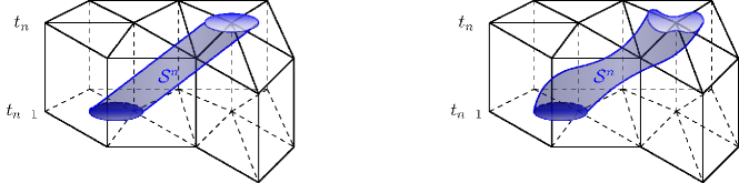
Fig. 1: Illustration of the local space-time triangulation $\mathcal{Q}_{h}^{\mathcal{S}}$ in one time slab. In the left picture we have a constant $\mathbf{w}$, hence (14) is satisfied.

The finite element method reads: Find $u_{h}\in W_{h}$ such that

$$\left\langle\dot{u}_{h},v_{h}\right\rangle_{b}+a(u_{h},v_{h})+d(u_{h},v_{h})=(f,v_{h})_{0}\quad\text{for all}~{}~{}v_{h}\in W_{h}.$$ (17)

As usual in time-DG methods, the initial condition for $u_{h}(\cdot,0)$ is treated in a weak sense. Due to $u_{h}\in H^{1}(Q_{n})$ for $n=1,\dots,N$, the first term in (17) can be written as

$$\left\langle\dot{u}_{h},v_{h}\right\rangle_{b}=\sum_{n=1}^{N}\int_{t_{n-1}}^{t_{n}}\int_{\Gamma(t)}(\frac{\partial u_{h}}{\partial t}+\mathbf{w}\cdot\nabla u_{h})v_{h}ds\,dt.$$ (18)

In the (very unlikely) case that $\Gamma(t)$ is a face of two tetrahedra $T_{1}$,$T_{2}$ and both $T_{1}\times I_{n}$ and $T_{2}\times I_{n}$ are contained in $\mathcal{Q}_{h}^{\mathcal{S}}$, we use a simple averaging in the evaluation of $\mathbf{w}\cdot\nabla u_{h}$ in (18). Recall that the solution of the continuous problem (3) satisfies the zero mean condition (2), which corresponds to the mass conservation law valid for the original problem (1). We investigate whether the condition (2) is preserved for the finite element formulation (17).

Assume that $u_{h}$ is a solution of (17). Denote $\bar{u}_{h}(t)=\int_{\Gamma(t)}u_{h}ds$. We have $\int_{\Gamma(t)}f\,ds=0$ for all $t>0$. In (17), set $v_{h}=1$ for $t\leq t_{n}$ and $v_{h}=0$ for $t>t_{n}$. This implies $\bar{u}_{h,-}(t_{n}):=\int_{\Gamma(t_{n})}u_{-}^{n}\,ds=0$ for $n=0,1,\dots$. Setting $v_{h}=t-t_{n-1}$ for $t_{n-1}\leq t\leq t_{n}$ and $v_{h}=0$ otherwise, we additionally get $\int_{t_{n-1}}^{t_{n}}\bar{u}_{h}(t)\,dt=0$. Summarizing, we obtain the following:

$$\bar{u}_{h,-}(t_{n})=0\quad\text{and}\quad\int_{t_{n-1}}^{t_{n}}\bar{u}_{h}(t)\,dt=0,\quad n=1,2,\dots.$$ (19)

For a stationary surface, $\bar{u}_{h}(t)$ is a piecewise affine function and thus (19) implies $\bar{u}_{h}(t)\equiv 0$, i.e., we have exact mass conservation on the discrete level. If the surface evolves, the finite element method is not necessarily mass conserving: (19) holds, but $\bar{u}_{h}(t)\neq 0$ may occur for $t_{n-1}\leq t<t_{n}$. To enforce a better mass conservation and enhance stability of the finite element method, cf. Remark 4.1, we introduce a consistent stabilizing term involving the quantity $\bar{u}_{h}(t)$ to the discrete bilinear form. More precisely, define

$$a_{\sigma}(u,v):=a(u,v)+\sigma\int_{0}^{T}\bar{u}(t)\bar{v}(t)\,dt,\quad\sigma\geq 0.$$ (20)

Instead of (17) we consider the stabilized version: Find $u_{h}\in W_{h}$ such that

$$\left\langle\dot{u}_{h},v_{h}\right\rangle_{b}+a_{\sigma}(u_{h},v_{h})+d(u_{h},v_{h})=(f,v_{h})_{0}\quad\text{for all}~{}~{}v_{h}\in W_{h}.$$ (21)

As mentioned above, taking $\sigma>0$ we expect both a stabilizing effect and an improved mass conservation property. Adding this stabilization term does not lead to significant additional computational costs for computing the stiffness matrix, cf. Section 3.1.

For the solution $u\in W$ of (15), the stabilization term vanishes: $\bar{u}(t)=0$. Therefore the error $e=u-u_{h}$ of the finite element method (21) satisfies the Galerkin orthogonality relation:

$$\left\langle\dot{e},v_{h}\right\rangle_{b}+a_{\sigma}(e,v_{h})+d(e,v_{h})=0\quad\text{for all}~{}~{}v_{h}\in W_{h}.$$ (22)

3.1 Implementation aspects

We comment on a few implementation aspects. More details are found in the recent article [15].

By choosing the test functions $v_{h}$ in (21) per time slab, as in standard space-time DG methods, one obtains an implicit time stepping algorithm. Two main implementation issues are the approximation of the space-time integrals in the bilinear form $\left\langle\dot{u}_{h},v_{h}\right\rangle_{b}+a_{\sigma}(u_{h},v_{h})$ and the representation of the finite element trace functions in $W_{h}$. To approximate the integrals, one makes use of the transformation formula (5) converting space-time integrals to surface integrals over $\mathcal{S}$, and next one approximates $\mathcal{S}$ by a ‘discrete’ surface $\mathcal{S}^{h}$; this is done locally, i.e. time slab per time slab. The approximate surface $\mathcal{S}^{h}$ can be the zero level of $\phi_{h}\in W_{\hat{h}}$, where $\phi_{h}$ is a bilinear finite element approximation of a level set function $\phi(x,t)$, the zero level of which is the surface $\mathcal{S}$. To reduce the “geometric error” it may be efficient to determine $\phi_{h}\in W_{\hat{h}}$ in a finite element space with mesh size $\hat{h}<h$, $\hat{\Delta t}<\Delta t$, e.g., $\hat{h}=\frac{1}{2}h$, $\hat{\Delta t}=\frac{1}{2}\Delta t$ (one regular refinement of the given outer space-time mesh). Within each space-time prism $T\times I_{n}\in\mathcal{Q}_{h}^{\mathcal{S}}$ the zero level of $\phi_{h}\in W_{\hat{h}}$ can be represented as a union of tetrahedra, cf. [15], and standard quadrature formulas can be used. Results of numerical experiments obtained using such treatment of integrals over $\mathcal{S}$ are reported in [15, 16, 26].

For the representation of the finite element functions in $W_{h}$ it is natural to use traces of the standard nodal basis functions in the volume space-time finite element space $V_{h}$. In general, these trace functions form a frame in $W_{h}$. A finite element surface solution is represented as a linear combination of the elements from this frame. Linear systems resulting in every time step may have more than one solution, but every solution yields the same trace function, which is the unique solution of (21). If $\Delta t\sim h$ and $\|\mathbf{w}\|_{L^{\infty}(\mathcal{S})}=\mathcal{O}(1)$ then the number of tetrahedra $T\in\mathcal{T}_{n}$ that are intersected by $\Gamma(t)$, $t\in I_{n}$, is of the order $\mathcal{O}(h^{-2})$. Hence, per time step the linear systems have $\mathcal{O}(h^{-2})$ unknowns, which is the same complexity as a discretized spatially two-dimensional elliptic problem. Note that although we derived the method in $\mathbb{R}^{3+1}$, due to the time stepping and the trace operation, the discrete problems have two-dimensional complexity. Since the discrete problems have a complexity of (only) $\mathcal{O}(h^{-2})$ it may be efficient to use a sparse direct solver for computing the discrete solution. Linear algebra aspects of the surface finite element method have been addressed in [24] and will be further investigated in future work.

The stabilization term in (20) does not cause significant additional computational work. In one time slab it has the form $\int_{t_{n-1}}^{t_{n}}\bar{u}(t)\bar{v}(t)\,dt$. Let $\phi_{i}$, $1\leq i\leq M$, denote the nodal basis functions in the outer space $V_{h}$, then the $M\times M$- matrix representing this bilinear form has entries $\int_{t_{n-1}}^{t_{n}}\int_{\Gamma(t)}\phi_{j}\,ds\int_{\Gamma(t)}\phi_{i}\,ds\,dt$. If quadrature for $\int_{t_{n-1}}^{t_{n}}$, with nodes $\xi_{1},\ldots,\xi_{k}\in[t_{n-1},t_{n}]$, is applied this results in a stabilization matrix of the form $S=\sum_{r=1}^{k}\alpha_{r}z_{r}z_{r}^{T}$, with $\alpha_{r}\in\mathbb{R}$, $z_{r}\in\mathbb{R}^{M}$. The vector $z_{r}$ has entries $(z_{r})_{i}=\int_{\Gamma(\xi_{r})}\phi_{i}(s,\xi_{r})\,ds$. We need only a few quadrature points, e.g. $k=2$, hence $S$ is a sum of only a few rank one matrices. Since the stabilization matrix is symmetric positive semi-definite it also improves the conditioning of the stiffness matr ix.

4 Stability of the finite element method

We present a stability analysis of the discrete problem (21) for the positive definite case, cf. Remark 2.3. In Remark 4.1 below we explain why we restrict ourselves to the positive definite case and comment on the role of the stabilization. We introduce the following mesh-dependent norm:

$$|\!|\!|u|\!|\!|_{h}:=\left(\max_{n=1,\dots,N}\|u_{-}^{n}\|_{t^{n}}^{2}+\sum_{n=1}^{N}\|[u]^{n-1}\|_{t_{n-1}}^{2}+\|u\|_{H}^{2}\right)^{\frac{1}{2}}.$$

Theorem 4.

Assume (14) and take $\sigma\geq\frac{\nu_{d}}{2}\max\limits_{t\in[0,T]}\frac{c_{F}(t)}{|\Gamma(t)|}$, where $c_{F}(t)$ is defined in (12). Then the inf-sup estimate

$$\inf_{u\in W^{b}}\sup_{v\in W^{b}}\frac{\left\langle\dot{u},v\right\rangle_{b}+a_{\sigma}(u,v)+d(u,v)}{|\!|\!|v|\!|\!|_{h}|\!|\!|u|\!|\!|_{h}}\geq c_{s}$$ (23)

and the ellipticity estimate

$$\left\langle\dot{u},u\right\rangle_{b}+a_{\sigma}(u,u)+d(u,u)\geq 2c_{s}\left(\|u_{-}^{N}\|_{T}^{2}+\sum_{n=1}^{N}\|[u]^{n-1}\|_{t_{n-1}}^{2}+\|u\|_{H}^{2}\right)$$ (24)

for all $u\in W^{b}$ hold, with $c_{s}=\frac{1}{4}\min\{1,\nu_{d},c_{0}\}$ and $c_{0}$ from (14). The results in (23), (24) also hold with $W^{b}$ replaced by $W_{h}$.

Proof.

Take $u\in W^{b}$, $u\neq 0$, and let $M\in\{1,\dots,N\}$. Set $\tilde{u}=u$ for $t\in(0,t_{M}]$ and $\tilde{u}=0$ for $t\in(t_{M},T)$. Applying partial integration on every time interval we get

$$\left\langle\dot{u},\tilde{u}\right\rangle_{b}=\frac{1}{2}\sum_{n=1}^{M}\Big{(}\|u_{-}^{n}\|_{t_{n}}^{2}-\|u_{+}^{n-1}\|_{t_{n-1}}^{2}\Big{)}-\frac{1}{2}\int_{0}^{t_{M}}({\operatorname{div_{\Gamma}}}\mathbf{w},u^{2})_{\Gamma(t)}\,dt.$$

It is also straightforward to derive

$$d(u,\tilde{u})=-\frac{1}{2}\sum_{n=1}^{M}\Big{(}\|u_{-}^{n}\|_{t_{n}}^{2}-\|u_{+}^{n-1}\|_{t_{n-1}}^{2}\Big{)}+\frac{1}{2}\|u_{-}^{M}\|_{t_{M}}^{2}+\frac{1}{2}\sum_{n=1}^{M}\|[u]^{n-1}\|_{t_{n-1}}^{2}.$$

The Friedrichs inequality (12) yields

$$\int_{\Gamma(t)}|\nabla_{\Gamma}u|^{2}\,ds\geq c_{F}(t)\big{(}\int_{\Gamma(t)}u^{2}\,ds-\frac{1}{|\Gamma(t)|}\bar{u}^{2}(t)\big{)}.$$

Using this, we get

$$a_{\sigma}(u,\tilde{u})=\int_{0}^{t_{M}}\nu_{d}\|\nabla_{\Gamma}u\|^{2}_{L^{2}(\Gamma(t))}+({\operatorname{div_{\Gamma}}}\mathbf{w},u^{2})_{L^{2}(\Gamma(t))}+\sigma\bar{u}(t)^{2}\,dt$$

$$\geq\int_{0}^{t_{M}}\frac{1}{2}(\nu_{d}c_{F}+2{\operatorname{div_{\Gamma}}}\mathbf{w},u^{2})_{L^{2}(\Gamma(t))}+(\sigma-\frac{\nu_{d}}{2}\frac{c_{F}(t)}{|\Gamma(t)|})\bar{u}(t)^{2}+\frac{\nu_{d}}{2}\|\nabla_{\Gamma}u\|^{2}_{L^{2}(\Gamma(t))}\,dt$$

$$\geq\int_{0}^{t_{M}}\frac{1}{2}(\nu_{d}c_{F}+2{\operatorname{div_{\Gamma}}}\mathbf{w},u^{2})_{L^{2}(\Gamma(t))}+\frac{\nu_{d}}{2}\|\nabla_{\Gamma}u\|^{2}_{L^{2}(\Gamma(t))}\,dt.$$

Combining the relations above and using (14), we get

$$\left\langle\dot{u},\tilde{u}\right\rangle_{b}+a_{\sigma}(u,\tilde{u})+d(u,\tilde{u})\geq\frac{1}{2}\left(\|u_{-}^{M}\|_{t_{M}}^{2}+\sum_{n=1}^{M}\|[u]^{n-1}\|_{t_{n-1}}^{2}\right.\\ \left.+\int_{0}^{t_{M}}c_{0}\|u\|^{2}_{L^{2}(\Gamma(t))}+\nu_{d}\|\nabla_{\Gamma}u\|^{2}_{L^{2}(\Gamma(t))}\,dt\right).$$ (25)

Taking $M=N$ in this inequality proves (24). Let $M$ be such that $\|u_{-}^{M}\|_{t^{M}}=\max_{n=1,\dots,N}\|u_{-}^{n}\|_{t^{n}}^{2}$. Setting $v=\tilde{u}+u$, using (25) and performing obvious computations gives (23). Since $W_{h}\subset W^{b}$ and $u\in W_{h}\,\Rightarrow\,\tilde{u}\in W_{h}$, the results in (23), (24) also hold on the finite element subspace. ∎

In this stability result there are no restrictions on the size of $h$ and $\Delta t$. In particular the stability is guaranteed even if $\Delta t$ is large. This is in agreement with the strong robustness of the method, observed in the numerical experiments in [15, 26, 16].

Remark 4.1.

We comment on the assumptions we use in Theorem 4. An inf-sup result in $W^{b}$, similar to (23), can also be derived for the general (indefinite) case, i.e., without assuming (14), and without stabilization. Such a result is given in Lemma 5.2 in [26]. The proof uses a test function of the form $v=\mu e^{-\gamma t}u+z$, with a suitable $\mu>0,\,\gamma>0$ and $z\in W^{b}$. The factor $e^{-\gamma t}$ is used to control the term $({\operatorname{div_{\Gamma}}}\mathbf{w}u,u)_{0}$. Of course, the stability constant then depends on $T$ and deteriorates for $T\to\infty$. For the discrete space $W_{h}$, however, we are not able to derive a stability result for the general (indefinite) case. The key point is that for $u_{h}\in W_{h}$ a test function of the form $e^{-\gamma t}u_{h}$ is not allowed, since it is not an element of the test space $W_{h}$. Using an approximation (interpolation or projection) of $e^{-\gamma t}u_{h}$ in the finite element space we are not able to get sufficient control of the term $({\operatorname{div_{\Gamma}}}\mathbf{w}u,u)_{0}$. A similar difficulty, for the general problem, arises if one applies a discrete analogon of the Gronwall argument outlined in Remark 2.2: Let $u=u_{h}\in W_{h}$ be a finite element function. For the corresponding test function one can take $v=\tilde{u}$ as in the proof above, i.e., $v=u_{|[0,t_{M}]}$. Taking $\sigma=0$ we obtain

$$\begin{split}&\frac{1}{2}\|u_{-}^{M}\|_{t_{M}}^{2}+\frac{1}{2}\sum_{n=1}^{M}\|[u]^{n-1}\|_{t_{n-1}}^{2}+\nu_{d}\int_{0}^{t_{M}}\int_{\Gamma(t)}(\nabla_{\Gamma}u)^{2}\,ds\,dt\\ &=\int_{0}^{t_{M}}\int_{\Gamma(t)}fu\,ds\,dt-\frac{1}{2}\int_{0}^{t_{M}}\int_{\Gamma(t)}{\operatorname{div_{\Gamma}}}\mathbf{w}u^{2}\,ds\,dt.\end{split}$$

Define $h(t):=\frac{1}{2}\int_{\Gamma(t)}u^{2}\,ds+\sum_{n=1}^{M}\|[u]^{n-1}\|_{t_{n-1}}^{2}+\nu_{d}\int_{0}^{t}\int_{\Gamma(\tau)}(\nabla_{\Gamma}u)^{2}\,dsd\tau$, for $t\in(t_{M-1},t_{M}]$, $M=1,\ldots N$. With similar arguments as in Remark 2.2 we get the estimate

$$h(t_{M})\leq\frac{1}{2}\|f\|_{0}^{2}+(1+\|{\operatorname{div_{\Gamma}}}\mathbf{w}\|_{L^{\infty}(\mathcal{S})})\int_{0}^{t_{M}}h(\tau)\,d\tau,\quad M=1,\ldots,N,$$

cf. (11). Define $a_{M}=h(t_{M})$. For a discrete Gronwall lemma we need an inequality of the form $a_{M}\leq c+\sum_{1\leq k<M}g_{k}a_{k}$, $M=1,\ldots,N$. In our case we have to control $\int_{0}^{t_{M}}h(\tau)\,d\tau$ by the values $h(t_{k})$, $k=0,\ldots,M$. For a stationary $\Gamma(t)$, this can be realized using the fact that $u$ is linear w.r.t. $t$ on $I_{n}$. For an evolving $\Gamma(t)$, however, the function $h(t)$ can have rather general behavior and it is not clear under which reasonable assumptions the integral can be bounded by the function values $h(t_{k})$.

In view of these observations we restrict analysis to the nicer positive definite case, hence we assume that (14) holds. As mentioned in Remark 2.3, condition (14) is not sufficient for $A$ to be positive definite on $W_{h}$. The difficulty comes from the functions $u(x,t)$ that are constant in spatial directions. For the continuous case we dealt with this problem by restricting to the subspace $\widetilde{W}$, cf. (13). In case of an evolving $\Gamma(t)$, requiring the discrete solution $u_{h}$ to lie in $\widetilde{W}$ is a too strong condition, which leads to an unacceptable reduction of the degrees of freedom (often, only $u_{h}=0$ is allowed). This is the reason, why we introduce the stabilization. For $\sigma$ sufficiently large the corresponding stabilized operator $A_{\sigma}$ is positive definite on $W_{h}$. In numerical experiments we observe that in general $\sigma=0$ results in a stable method. We have the following heuristic explanation for this. The discrete solution remains the same if we restrict the discretization to the subspace $\widetilde{W}_{h}\subset W_{h}$ of functions that sati sfy (19). The distance of this space $\widetilde{W}_{h}$ to $\widetilde{W}^{b}=\{\,u\in W^{b}~{}|~{}\bar{u}(t)=0\,\}$ is expected to be small. On the latter space the operator $A$ without stabilization is positive definite (if (14) holds) and thus it is plausible that this positive definiteness holds on $\widetilde{W}_{h}$, too.

The ellipticity result (24) is sufficient for existence of a unique solution and (23) yields a priori bound in $|\!|\!|\cdot|\!|\!|_{h}$ norm. We summarize this in the following proposition.

Proposition 5.

Assume (14) and take $\sigma$ as in Theorem 4. Then the discrete problem (21) has a unique solution $u_{h}\in W_{h}$. For $u_{h}$ the a priori estimate

$$|\!|\!|u_{h}|\!|\!|_{h}\leq c_{s}^{-1}\|f\|_{0}.$$ (26)

holds, with $c_{s}$ as in Theorem 4.

5 Continuity result

We derive continuity results for the bilinear form of the finite element method.

Lemma 6.

For any $e,v\in W^{b}$ the following holds, with constants $c$ independent of $e,v,h,N$:

$$|\left\langle\dot{e},v\right\rangle_{b}+a_{\sigma}(e,v)+d(e,v)| \leq c|\!|\!|v|\!|\!|_{h}(\|e\|_{W^{b}}+\sum_{n=0}^{N-1}\|[e]^{n}\|_{t^{n}}),$$ (27)

$$|\left\langle\dot{e},v\right\rangle_{b}+a_{\sigma}(e,v)+d(e,v)| \leq c|\!|\!|e|\!|\!|_{h}(\|v\|_{W^{b}}+\sum_{n=1}^{N-1}\|[v]^{n}\|_{t^{n}}+\|v\|_{T}).$$ (28)

Proof.

The stabilizing term in $a_{\sigma}(e,v)$ is estimated as follows:

$$\left|\sigma\int_{0}^{T}\int_{\Gamma(t)}e\,dx\int_{\Gamma(t)}vdx\,dt\right| \leq\sigma\int_{0}^{T}|\Gamma(t)|\left(\int_{\Gamma(t)}e^{2}dx\right)^{\frac{1}{2}}\left(\int_{\Gamma(t)}v^{2}dx\right)^{\frac{1}{2}}\,dt$$ (29)

$$\leq\sigma\max\limits_{t\in[0,T]}|\Gamma(t)|\|e\|_{0}\|v\|_{0}.$$

The material derivative term is treated using integration by part:

$$\left\langle\dot{e},\right. \left.v\right\rangle_{b}=\sum_{n=1}^{N}\Big{(}(e_{-}^{n},v_{-}^{n})_{t_{n}}-(e_{+}^{n-1},v_{+}^{n-1})_{t_{n-1}}\Big{)}-({\operatorname{div_{\Gamma}}}\mathbf{w}\,e,v)_{0}-\left\langle\dot{v},e\right\rangle_{b}$$

$$=-\sum_{n=1}^{N}([e]^{n-1},v_{+}^{n-1})_{t_{n-1}}-\sum_{n=1}^{N-1}([v]^{n},e_{-}^{n})_{t_{n}}+(e_{-}^{N},v)_{T}-({\operatorname{div_{\Gamma}}}\mathbf{w}\,e,v)_{0}-\left\langle\dot{v},e\right\rangle_{b}$$

$$=-d(e,v)-\sum_{n=1}^{N-1}([v]^{n},e_{-}^{n})_{t_{n}}+(e_{-}^{N},v)_{T}-({\operatorname{div_{\Gamma}}}\mathbf{w}\,e,v)_{0}-\left\langle\dot{v},e\right\rangle_{b}.$$

Now we use the relation $\left\langle\dot{v},e\right\rangle_{b}=\sum_{n=1}^{N}\left\langle\dot{v}_{n},e_{n}\right\rangle\$ and the Cauchy inequality to estimate

$$\begin{split}|\left\langle\dot{e},v\right\rangle_{b}+d(e,v)|&\leq\|e_{-}^{N}\|_{T}\|v\|_{T}+\alpha_{\infty}\|e\|_{0}\|v\|_{0}+\|e\|_{H}\left(\sum_{n=1}^{N}\|\dot{v}_{n}\|^{2}_{H^{\prime}_{n}}\right)^{\frac{1}{2}}\\ &+\max_{n=1,\dots,N-1}\|e_{-}^{n}\|_{t_{n}}\sum_{n=1}^{N-1}\|[v]^{n}\|_{t_{n}}.\end{split}$$ (30)

Combining (29), (30), and $a(e,v)\leq\nu_{d}\|\nabla_{\Gamma}e\|_{0}\|\nabla_{\Gamma}v\|_{0}+\alpha_{\infty}\|e\|_{0}\|v\|_{0}$, we get

$$|\left\langle\dot{e},v\right\rangle_{b}+a_{\sigma}(e,v)+d(e,v)|$$

$$\leq\|e_{-}^{N}\|_{T}\|v\|_{T}+(2\alpha_{\infty}+\sigma\max\limits_{t\in[0,T]}|\Gamma(t)|)\|e\|_{0}\|v\|_{0}+\|e\|_{H}\left(\sum_{n=1}^{N}\|\dot{v}_{n}\|^{2}_{H^{\prime}_{n}}\right)^{\frac{1}{2}}$$

$$+\nu_{d}\|\nabla_{\Gamma}e\|_{0}\|\nabla_{\Gamma}v\|_{0}+\max_{n=1,\dots,N-1}\|e_{-}^{n}\|_{t_{n}}\sum_{n=1}^{N-1}\|[v]^{n}\|_{t_{n}}.$$

The Cauchy inequality and the definition of the norms $|\!|\!|e|\!|\!|_{h}$, $\|v\|_{W^{b}}$ imply the result in (28). The inequality in (27) is proved by the same arguments, but skipping the integration by parts step.  ∎

The norm $|\!|\!|\cdot|\!|\!|_{h}$ is weaker than the norm $\|\cdot\|_{W}$ used for the stability analysis of the original ‘differential’ weak formulation (7), since the latter norm provides control over the material derivative in $H^{\prime}$. For the discrete solution we can establish control over the material derivative only in a weaker sense, namely in a space dual to the discrete space. Indeed, using estimates as in the proof of Lemma 6 we get

$$|a_{\sigma}(u_{h},v)|\\ \leq|\!|\!|u_{h}|\!|\!|_{h}\left((\alpha_{\infty}+\sigma\max\limits_{t\in[0,T]}|\Gamma(t)|)^{2}\|v\|_{0}^{2}+\nu_{d}^{2}\|\nabla_{\Gamma}v\|_{0}^{2}\right)^{\frac{1}{2}}\leq c\,|\!|\!|u_{h}|\!|\!|_{h}\|v\|_{H},$$

and thus for the discrete solution $u_{h}\in W_{h}$ of (21) one obtains, using (26):

$$\sup_{v\in W_{h}}\frac{\left\langle\dot{u}_{h},v\right\rangle_{b}+d(u_{h},v)}{\|v\|_{H}}=\sup_{v\in W_{h}}\frac{(f,v_{h})_{0}-a_{\sigma}(u_{h},v)}{\|v\|_{H}}\leq c\|f\|_{0}.$$ (31)

6 Discretization error analysis

In this section we prove an error bound for the discrete problem (21). The analysis is based on the usual arguments, namely the stability estimate derived above combined with the Galerkin orthogonality and interpolation error bounds. The surface finite element space is the trace of an outer volume finite element space $V_{h}$. For the analysis of the discretization error in the surface finite element space we use information on the approximation quality of the outer space. Hence, we need a suitable extension procedure for smooth functions on the space-time manifold $\mathcal{S}$. This topic is addressed in subsection 6.1.

6.1 Extension of functions defined on $\mathcal{S}$

For a function $u\in H^{2}(\mathcal{S})$ we need an extension $u^{e}\in H^{2}(U)$, where $U$ is a neighborhood in $\mathbb{R}^{4}$ that contains the space-time manifold $\mathcal{S}$. Below we introduce such an extension and derive some properties that we need in the analysis. We extend $u$ in a spatial normal direction to $\Gamma(t)$ for every $t\in[0,T]$. For this procedure to be well-defined and the properties to hold, we need sufficient smoothness of the manifold $\mathcal{S}$. We assume $\mathcal{S}$ to be a three-dimensional $C^{3}$-manifold in $\mathbb{R}^{4}$.

For some $\delta>0$ let

$$U=\{\,\mathbf{x}:=(x,t)\in\mathbb{R}^{3+1}~{}|~{}{\rm dist}(x,\Gamma(t))<\delta\,\}$$ (32)

be a neighborhood of $\mathcal{S}$. The value of $\delta$ depends on curvatures of $\mathcal{S}$ and will be specified below. Let $d:U\rightarrow\mathbb{R}$ be the signed distance function, $|d(x,t)|:={\rm dist}(x,\Gamma(t))$ for all $\mathbf{x}\in U$. Thus, $\mathcal{S}$ is the zero level set of $d$. The spatial gradient $\mathbf{n}_{\Gamma}=\nabla_{x}d\in\mathbb{R}^{3}$ is the exterior normal vector for $\Gamma(t)$. The normal vector for $\mathcal{S}$ is

$$\mathbf{n}_{\mathcal{S}}=\nabla d/\|\nabla d\|=\frac{1}{\sqrt{1+V_{\Gamma}^{2}}}(\mathbf{n}_{\Gamma},-V_{\Gamma})^{T}\in\mathbb{R}^{4},\quad V_{\Gamma}=\mathbf{w}\cdot\mathbf{n}_{\Gamma}.$$

Recall that $V_{\Gamma}$ is the normal velocity of the evolving surface $\Gamma(t)$. The normal $\mathbf{n}_{\Gamma}$ has a natural extension given by $\mathbf{n}(\mathbf{x}):=\nabla_{x}d(\mathbf{x})\in\mathbb{R}^{3}$ for all $\mathbf{x}\in U$. Thus, $\mathbf{n}=\mathbf{n}_{\Gamma}$ on $\mathcal{S}$ and $\|\mathbf{n}(\mathbf{x})\|=1$ for all $\mathbf{x}\in U$. The spatial Hessian of $d$ is denoted by $\mathbf{H}\in\mathbb{R}^{3\times 3}$. The eigenvalues of $\mathbf{H}$ are $\kappa_{1}(x,t),\kappa_{2}(x,t)$, and 0. For $x\in\Gamma(t)$ the eigenvalues $\kappa_{i}(x,t)$, $i=1,2$, are the principal curvatures of $\Gamma(t)$. Due to the smoothness assumptions on $\mathcal{S}$, the principal curvatures are uniformly bounded in space and time:

$$\sup_{t\in[0,T]}\sup_{x\in\Gamma(t)}(|\kappa_{1}(x,t)|+|\kappa_{2}(x,t)|)\leq\kappa_{\max}.$$

We introduce a local coordinate system by using the projection $\mathbf{p}:\,U\rightarrow\mathcal{S}$:

$$\mathbf{p}(\mathbf{x})=\mathbf{x}-d(\mathbf{x})(\mathbf{n}(\mathbf{x}),0)^{T}=\big{(}x-d(x,t)\mathbf{n}(x,t),t\big{)}\quad\text{for all}~{}~{}\mathbf{x}=(x,t)\in U.$$

For $\delta$ sufficiently small, namely $\delta\leq\kappa_{\max}^{-1}$, the decomposition $\mathbf{x}=\mathbf{p}(\mathbf{x})+d(\mathbf{x})\big{(}\mathbf{n}(\mathbf{x}),0\big{)}$ is unique for all $\mathbf{x}\in U$ ([14], Lemma 14.16).

The extension operator is defined as follows. For a function $v$ on $\mathcal{S}$ we define

$$v^{e}(\mathbf{x}):=v(\mathbf{p}(\mathbf{x}))\quad\text{for all}~{}~{}\mathbf{x}\in U,$$ (33)

i.e., $v$ is extended along spatial normals on $\mathcal{S}$.

We need a few relations between surface norms of a function and volumetric norms of its extension. Define $\mu(\mathbf{x}):=\big{(}1-d(\mathbf{x})\kappa_{1}(\mathbf{x})\big{)}\big{(}1-d(\mathbf{x})\kappa_{2}(\mathbf{x})\big{)}$ for $\mathbf{x}\in U$. From (2.20), (2.23) in [4] we have

$$\mu(\mathbf{x})\mathrm{d}x=\mathrm{d}s(\mathbf{p}(\mathbf{x}))\,\mathrm{d}r\,\quad\mathbf{x}\in U,$$

where $\mathrm{d}x$ is the volume measure in $\mathbb{R}^{3}$, $\mathrm{d}s$ the surface measure on $\Gamma(t)$, and $r$ the local coordinate at $y\in\Gamma(t)$ in the (orthogonal) direction $\mathbf{n}_{\Gamma}(y)$. Assume $\delta\leq\frac{1}{4}\kappa_{\max}^{-1}$. Using the relation $\kappa_{i}(\mathbf{x})=\frac{\kappa_{i}(\mathbf{p}(\mathbf{x}))}{1+d(\mathbf{x})\kappa_{i}(\mathbf{p}(\mathbf{x}))}$, $i=1,2$, $\mathbf{x}\in U$, ((2.5) in [4]) one obtains $\frac{9}{16}\leq\mu(\mathbf{x})\leq\frac{25}{16}$ for all $\mathbf{x}\in U$. Now let $v$ be a function defined on $\mathcal{S}$ and $w$, defined on $U$, given by $w(\mathbf{x})=g(\mathbf{x})v(\mathbf{p}(\mathbf{x}))$, with a function $g$ that is bounded on $U$: $\|g\|_{L^{\infty}(U)}\leq c_{g}<\infty$. An example is the pair $w=v^{e}$ and $v$ given in (33), with $g\equiv 1$. For $v,w$ we have the following, with $U(t)=\{\,x\in\mathbb{R}^{3}~{}|~{}{\rm dist}(x,\Gamma(t))<\delta\,\}$ the cross-section of $U$ for some $t\in[0,T]$ and a local coordinate system denoted by $\mathbf{x}=(\mathbf{p}(\mathbf{x}),r)$:

$$\begin{split}&\|w\|_{L^{2}(U)}^{2}=\int_{U}w^{2}(\mathbf{x})\,\mathrm{d}\mathbf{x}\leq c\int_{0}^{T}\int_{U(t)}w(\mathbf{x})^{2}\mu(\mathbf{x})\,\mathrm{d}x\mathrm{d}t\\ &\leq c\,\int_{0}^{T}\int_{U(t)}v(\mathbf{p}(\mathbf{x}))^{2}\mu(\mathbf{x})\,\mathrm{d}x\mathrm{d}t=c\,\int_{0}^{T}\int_{-\delta}^{\delta}\int_{\Gamma(t)}v(\mathbf{p}(\mathbf{x}))^{2}\,\mathrm{d}s(\mathbf{p}(\mathbf{x}))\mathrm{d}r\mathrm{d}t\\ &\leq c\,\delta\int_{0}^{T}\int_{\Gamma(t)}v^{2}\,\mathrm{d}s\mathrm{d}t\leq c\delta\|v\|_{L^{2}(\mathcal{S})}^{2}.\end{split}$$ (34)

The constant $c$ in the estimate above depends only on the smoothness of $\mathcal{S}$ and on $c_{g}$. If in addition $|g(\mathbf{x})|\geq c_{0}>0$ on $U$ holds, then we obtain the estimate $\|w\|_{L^{2}(U)}^{2}\geq c\delta\|v\|_{L^{2}(\mathcal{S})}^{2}$, with a constant $c>0$ depending only on $|V_{\Gamma}|$ and $c_{0}$. Using these results applied to $w=v^{e}$ as in (33) (i.e., $g\equiv 1)$, we obtain the equivalence

$$\|u^{e}\|_{L^{2}(U)}^{2}\simeq\delta\|u\|_{L^{2}(\mathcal{S})}^{2}\qquad\text{for all}~{}~{}u\in L^{2}(\mathcal{S}).$$ (35)

In the remainder of this section, for $u$ defined on $\mathcal{S}$, we derive bounds on derivatives of $u^{e}$ on $U$ in terms of the derivatives of $u$ on $\mathcal{S}$. We first recall a few elementary results. From

$$\nabla_{\mathcal{S}}u=(\mathbf{I}_{4\times 4}-\mathbf{n}_{\mathcal{S}}\mathbf{n}_{\mathcal{S}}^{T})\begin{pmatrix}\nabla_{x}u^{e}\\ u_{t}^{e}\end{pmatrix},\quad\nabla_{\Gamma(t)}u=(\mathbf{I}_{3\times 3}-\mathbf{n}_{\Gamma}\mathbf{n}_{\Gamma}^{T})\nabla_{x}u^{e},$$

one derives the following relations between tangential derivatives:

$$\nabla_{\Gamma(t)}u =\mathbf{B}\nabla_{\mathcal{S}}u,\quad\mathbf{B}:=[\mathbf{I}_{3\times 3},-V_{\Gamma}\mathbf{n}_{\Gamma}]\in\mathbb{R}^{3\times 4},$$ (36)

$$\dot{u} =(1+V_{\Gamma}^{2})(\nabla_{\mathcal{S}}u)_{4}+\mathbf{w}\cdot\nabla_{\Gamma(t)}u,$$ (37)

where $(\nabla_{\mathcal{S}}u)_{4}$ denotes the fourth entry of the vector $\nabla_{\mathcal{S}}u\in\mathbb{R}^{4}$. The spatial derivatives of the extended function can be written in terms of surface gradients (cf., e.g. (2.13) in [4]):

$$\nabla_{x}u^{e}(\mathbf{x})=(\mathbf{I}-d\mathbf{H})\nabla_{\Gamma(t)}u(\mathbf{p}(\mathbf{x}))=(\mathbf{I}-d\mathbf{H})\mathbf{B}\nabla_{\mathcal{S}}u(\mathbf{p}(\mathbf{x}))=:\mathbf{B}_{1}\nabla_{\mathcal{S}}u(\mathbf{p}(\mathbf{x})),$$ (38)

for $\mathbf{x}\in U$. This implies $\nabla_{x}u^{e}(\mathbf{x})=\nabla_{\Gamma(t)}u(\mathbf{p}(\mathbf{x}))=\nabla_{\Gamma(t)}u(\mathbf{x})$ for $\mathbf{x}\in\mathcal{S}$. For the time derivative we obtain

$$u^{e}_{t}(\mathbf{x})=\frac{\partial}{\partial t}(u^{e}\circ\mathbf{p})(\mathbf{x})=\frac{\partial}{\partial t}u^{e}(x-d(x,t)\mathbf{n}(x,t),t)\\ =u^{e}_{t}(\mathbf{p}(\mathbf{x}))-(d_{t}\mathbf{n}+d\mathbf{n}_{t})\cdot\nabla_{x}u^{e}(\mathbf{p}(\mathbf{x}))=u^{e}_{t}(\mathbf{p}(\mathbf{x}))-(d_{t}\mathbf{n}+d\mathbf{n}_{t})\cdot\nabla_{\Gamma(t)}u(\mathbf{p}(\mathbf{x})).$$ (39)

The time derivative $u^{e}_{t}$ on $\mathcal{S}$ can be represented in terms of surface quantities, cf. (37) :

$$u^{e}_{t}=\dot{u}-\mathbf{w}\cdot\nabla_{x}u^{e}=\dot{u}-\mathbf{w}\cdot\nabla_{\Gamma(t)}u=(1+V_{\Gamma}^{2})(\nabla_{\mathcal{S}}u)_{4}\quad\text{on}~{}\mathcal{S}.$$

Using this and (36) in (39) we obtain, for $\mathbf{x}\in U$,

$$u^{e}_{t}(\mathbf{x})=(1+V_{\Gamma}^{2})(\nabla_{\mathcal{S}}u(\mathbf{p}(\mathbf{x})))_{4}-(d_{t}\mathbf{n}+d\mathbf{n}_{t})\cdot\mathbf{B}\nabla_{\mathcal{S}}u(\mathbf{p}(\mathbf{x}))=:\mathbf{B}_{2}\cdot\nabla_{\mathcal{S}}u(\mathbf{p}(\mathbf{x})).$$ (40)

The matrices $\mathbf{B}_{1}$, $\mathbf{B}_{2}$ in (38), (40) depend only on geometric quantities related to $\mathcal{S}$ ($d$, $d_{t}$, $\mathbf{H}$, $V_{\Gamma}$, $\mathbf{n}$, $\mathbf{n}_{t}$). These quantities are uniformly bounded on $U$ due to the smoothness assumption on $\mathcal{S}$. Hence, from (38) and the result in (34) we obtain

$$\|\nabla u^{e}\|_{L^{2}(U)}^{2}\leq c\,\delta\|\nabla_{\mathcal{S}}u\|_{L^{2}(\mathcal{S})}^{2}\quad\text{for all}~{}u\in H^{1}(\mathcal{S}).$$ (41)

We need a similar result for the $H^{2}$ volumetric and surface norms. From (38) we get $\frac{\partial u^{e}}{\partial x_{i}}(\mathbf{x})=\mathbf{b}_{i}\cdot\nabla_{\mathcal{S}}u(\mathbf{p}(\mathbf{x}))$, $x\in U$, $i=1,2,3$, with $\mathbf{b}_{i}$ the $i$-th row of the matrix $\mathbf{B}_{1}$. For $z\in\{x_{1},x_{2},x_{3},t\}$ we get

$$\frac{\partial^{2}u^{e}}{\partial z\partial x_{i}}(\mathbf{x})=(\mathbf{b}_{i})_{z}\cdot\nabla_{\mathcal{S}}u(\mathbf{p}(\mathbf{x}))+\mathbf{b}_{i}(\nabla_{\mathcal{S}}\nabla_{\mathcal{S}}u)(\mathbf{p}(\mathbf{x}))\frac{\partial}{\partial z}\mathbf{p}(\mathbf{x}),\quad\mathbf{x}\in U.$$

Due to the smoothness assumption on $\mathcal{S}$ the vectors $\mathbf{b}_{i}$, $(\mathbf{b}_{i})_{z}$, $\frac{\partial}{\partial z}\mathbf{p}(\mathbf{x})$ have bounded $L^{\infty}$ norms on $U$ and application of (34) yields

$$\left\|\frac{\partial^{2}u^{e}}{\partial z\partial x_{i}}\right\|_{L^{2}(U)}^{2}\leq c\delta\Big{(}\sum_{|\mu|=2}\|\mathrm{D}^{\mu}_{\mathcal{S}}u\|_{L^{2}(\mathcal{S})}^{2}+\|\nabla_{\mathcal{S}}u\|_{L^{2}(\mathcal{S})}^{2}\Big{)}.$$

With similar arguments, using (40), one can derive the same bound for $\|\frac{\partial^{2}u^{e}}{\partial z\partial t}\|_{L^{2}(U)}^{2}$. Hence we conclude

$$\|u^{e}\|_{H^{2}(U)}^{2}\leq c\delta\|u\|_{H^{2}(\mathcal{S})}^{2}\quad\text{for all}~{}~{}u\in H^{2}(\mathcal{S}).$$ (42)

6.2 Interpolation error bounds

In this section, we introduce and analyze an interpolation operator. Recall that the local space-time triangulation $\mathcal{Q}_{h}^{\mathcal{S}}$ consists of cylindrical elements that are intersected by $\mathcal{S}$, cf. Fig. 1, and that the domain formed by these prisms is denoted by $Q^{\mathcal{S}}$. For $K\in\mathcal{Q}_{h}^{\mathcal{S}}$, the nonempty intersections are denoted by $\mathcal{S}_{K}=K\cap\mathcal{S}$. Let

$$I_{h}:C(Q^{\mathcal{S}})\to V_{h}$$

be the nodal interpolation operator. Since the triangulation may vary from time-slab to time-slab, the interpolant is in general discontinuous between the time-slabs.

In the remainder we take $\Delta t\sim h$. This assumption is made to avoid anisotropic interpolation estimates, which would significantly complicate the analysis for the case of surface finite elements.

We take a fixed neighborhood $U$ of $\mathcal{S}$ as in (32), with $\delta>0$ sufficiently small such that the analysis presented in section 6.1 is valid ($\delta\leq\frac{1}{4}\kappa_{\max}^{-1}$). The mesh is assumed to be fine enough to resolve the geometry of $\mathcal{S}$ in the sense that $\mathcal{Q}_{h}^{\mathcal{S}}\subset U$. We need one further technical assumption, which holds if the space time manifold $\mathcal{S}$ is sufficiently resolved by the outer (local) triangulation $\mathcal{Q}_{h}^{\mathcal{S}}$.

Assumption 6.1.

For $\mathcal{S}_{K}=K\cap\mathcal{S}$, $K\in\mathcal{Q}_{h}^{\mathcal{S}}$, we assume that there is a local orthogonal coordinate system $y=(z,\theta)$, $z\in\mathbb{R}^{3}$, $\theta\in\mathbb{R}$, such that $\mathcal{S}_{K}$ is the graph of a $C^{1}$ smooth scalar function, say $g_{K}$, i.e., $\mathcal{S}_{K}=\{\,(z,g_{K}(z))~{}|~{}z\in Z_{K}\subset\mathbb{R}^{3}\,\}$. The derivatives $\|\nabla g_{K}\|_{L^{\infty}(Z_{K})}$ are assumed to be uniformly bounded with respect to $K\in\mathcal{Q}_{h}^{\mathcal{S}}$ and $h$ . Finally it is assumed that the graph $\mathcal{S}_{K}$ either coincides with one of the three-dimensional faces of $K$ or it subdivides $K$ into exactly two subsets (one above and one below the graph of $g_{K}$).

The next lemma is essential for our analysis of the interpolation operator. This result was presented in [18, 19]. We include a proof because the 4D case is not discussed in [18, 19].

Lemma 7.

There is a constant $c$, depending only on the shape regularity of the tetrahedral triangulations $\mathcal{T}_{n}$ and the smoothness of $\mathcal{S}$, such that

$$\|v\|_{L^{2}(\mathcal{S}_{K})}^{2}\leq c(h^{-1}\|v\|_{L^{2}(K)}^{2}+h\|v\|_{H^{1}(K)}^{2})\quad\text{for all}~{}~{}v\in H^{1}(K),~{}K\in\mathcal{Q}_{h}^{\mathcal{S}}.$$ (43)

Proof.

We recall the following trace result (e.g. Thm. 1.1.6 in [2]) for a reference simplex $\widehat{K}$:

$$\|v\|_{L^{2}(\partial\widehat{K})}^{2}\leq c\|v\|_{L^{2}(\widehat{K})}\|v\|_{H^{1}(\widehat{K})}\quad\text{for all}~{}v\in H^{1}(\widehat{K}).$$

The Cauchy inequality and the standard scaling argument yield for $K\in\mathcal{Q}_{h}^{\mathcal{S}}$

$$\|v\|_{L^{2}(\partial K)}^{2}\leq c(h^{-1}\|v\|_{L^{2}(K)}^{2}+h\|v\|_{H^{1}(K)}^{2})\quad\text{for all}~{}~{}v\in H^{1}(K),$$ (44)

with a constant $c$ that depends only on the shape regularity of $K$. Take $K\in\mathcal{Q}_{h}^{\mathcal{S}}$ and let $\mathcal{S}_{K}=\{\,(z,g(z))~{}|~{}z\in Z_{K}\subset\mathbb{R}^{3}\,\}$ be as in Assumption 6.1. If $\mathcal{S}_{K}$ coincides with one of the three-dimensional faces of $K$ then (43) follows from (44). We consider the situation that the graph $\mathcal{S}_{K}$ divides $K$ into two nonempty subdomains $K_{i}$, $i=1,2$. Take $i$ such that $\mathcal{S}_{K}\subset\partial K_{i}$. Let $\mathbf{n}=(n_{1},\ldots,n_{4})^{T}$ be the unit outward pointing normal on $\partial K_{i}$. For $v\in H^{1}(K)$ the following holds, where ${\rm div}_{y}$ denotes the divergence operator in the $y=(z,\theta)$-coordinate system (cf. Assumption 6.1),

$$2\int_{K_{i}}v\frac{\partial v}{\partial\theta}\,dy =\int_{K_{i}}{\rm div}_{y}\begin{pmatrix}0\\ v^{2}\end{pmatrix}\,dy=\int_{\partial K_{i}}\mathbf{n}\cdot\begin{pmatrix}0\\ v^{2}\end{pmatrix}\,ds=\int_{\partial K_{i}}n_{4}v^{2}\,ds$$

$$=\int_{\mathcal{S}_{K}}n_{4}v^{2}\,ds+\int_{\partial K_{i}\setminus\mathcal{S}_{K}}n_{4}v^{2}\,ds.$$

On $\mathcal{S}_{K}$ the normal $\mathbf{n}$ has direction $(-\nabla_{z}g(z),1)^{T}$ and thus $n_{4}(y)=(\|\nabla_{z}g(z)\|^{2}+1)^{-\frac{1}{2}}$ holds. From Assumption 6.1 it follows that there is a generic constant $c$ such that $1\leq n_{4}(z)^{-1}\leq c$ holds. Using this we obtain

$$\int_{\mathcal{S}_{K}}v^{2}\,ds\leq c\int_{\mathcal{S}_{K}}n_{4}v^{2}\,ds\leq c\|v\|_{L^{2}(K_{i})}\|v\|_{H^{1}(K_{i})}+c\int_{\partial K_{i}\setminus\mathcal{S}_{K}}v^{2}\,ds$$

$$\leq c\|v\|_{L^{2}(K)}\|v\|_{H^{1}(K)}+c\int_{\partial K}v^{2}\,ds$$

$$\leq c(h^{-1}\|v\|_{L^{2}(K)}^{2}+h\|v\|_{H^{1}(K)}^{2})+c\int_{\partial K}v^{2}\,ds\leq c(h^{-1}\|v\|_{L^{2}(K)}^{2}+h\|v\|_{H^{1}(K)}^{2}),$$

where in the last inequality we used (44). ∎

We prove the following approximation result:

Theorem 8.

For sufficiently smooth $u$ defined on $\mathcal{S}$ we have:

$$\sum_{n=1}^{N}\|u-I_{h}u^{e}\|_{H^{k}(\mathcal{S}^{n})}^{2} \leq ch^{2(2-k)}\|u\|_{H^{2}(\mathcal{S})}^{2},\quad k=0,1,$$ (45)

$$\|u-(I_{h}u^{e})_{-}\|_{t^{n}} \leq ch^{2}\|u\|_{H^{2}(\Gamma(t^{n}))},~{}~{}n=1,\dots,N,$$

$$\|u-(I_{h}u^{e})_{+}\|_{t^{n}} \leq ch^{2}\|u\|_{H^{2}(\Gamma(t^{n}))},~{}~{}n=0,\dots,N-1.$$

The constants $c$ are independent of $u,h,N$.

Proof.

Since $\mathcal{S}$ is a smooth three-dimensional manifold, the embedding $H^{2}(\mathcal{S})\hookrightarrow C(\mathcal{S})$ holds. Hence $u\in C(\mathcal{S})$ implies $u^{e}\in C(U)$, and the nodal interpolant $I_{h}u^{e}$ is well defined. Define $v_{h}=(I_{h}u^{e})|_{\mathcal{S}}\in W_{h}$. Using Lemma 7, we obtain for $K\in\mathcal{Q}_{h}^{\mathcal{S}}$:

$$\|u-v_{h}\|_{L^{2}(\mathcal{S}_{K})}^{2}\leq c(h^{-1}\|u^{e}-I_{h}u^{e}\|_{L^{2}(K)}^{2}+h\|u^{e}-I_{h}u^{e}\|_{H^{1}(K)}^{2}).$$

Standard interpolation error bounds for $I_{h}$ and summing over all $K\in\mathcal{Q}_{h}^{\mathcal{S}}$ yields

$$\|u-v_{h}\|_{L^{2}(\mathcal{S})}^{2}\leq ch^{3}\|u^{e}\|_{H^{2}(\mathcal{Q}_{h}^{\mathcal{S}})}^{2}.$$

We use $\mathcal{Q}_{h}^{\mathcal{S}}\subset U$ and (42) to infer

$$\|u-v_{h}\|_{L^{2}(\mathcal{S})}^{2}\leq c\delta h^{3}\|u\|_{H^{2}(\mathcal{S})}^{2}.$$

Since we may assume $\delta\simeq h$, the result in (45) follows for $k=0$. The same technique is applied to show the result for $k=1$:

$$\|\nabla_{\mathcal{S}}(u-v_{h})\|_{L^{2}(\mathcal{S}_{K})}^{2}\leq c\|\nabla(u^{e}-I_{h}u^{e})\|_{L^{2}(\mathcal{S}_{K})}^{2}$$

$$\leq c(h^{-1}\|\nabla(u^{e}-I_{h}u^{e})\|_{L^{2}(K)}^{2}+h|\nabla(u^{e}-I_{h}u^{e})|_{H^{1}(K)}^{2})\leq ch\|u^{e}\|_{H^{2}(K)}^{2}.$$

Summing over all $K\in\mathcal{Q}_{h}^{\mathcal{S}}$ and using (42), with $\delta\simeq h$, then yields the first estimate in (45). The second and third estimates follow by similar arguments, using that $u^{e}$ is the extension in normal spatial direction and combining this with the three-dimensional version of Lemma 7 and standard interpolation error bounds for $I_{h}u^{e}_{|T}$, with $T$ a tetrahedron such that $K=T\times I_{n}\in\mathcal{Q}_{h}^{\mathcal{S}}$. ∎

6.3 Discretization error bound

The next theorem is the first main result of this paper. It shows optimal convergence in the $|\!|\!|\cdot|\!|\!|_{h}$ norm.

Theorem 9.

Let $u\in\overset{\circ}{W}$ be the solution of (7) and assume $u\in H^{2}(\mathcal{S})$, $u\in H^{2}(\Gamma(t))$ for all $t\in[0,T]$. Let $u_{h}\in W_{h}$ be the solution of the discrete problem (21) with a stabilization parameter $\sigma$ as in Theorem 4. The following error bound holds:

$$|\!|\!|u-u_{h}|\!|\!|_{h}\leq ch(\|u\|_{H^{2}(\mathcal{S})}+\sup_{t\in[0,T]}\|u\|_{H^{2}(\Gamma(t))}).$$

Proof.

For the solution $u\in H^{2}(\mathcal{S})$ let $e_{I}=u-(I_{h}u^{e})|_{\mathcal{S}}$ denote the interpolation error and $e=u-u_{h}$ the discretization error. The inf-sup stability result in (23) with $W^{b}$ replaced by $W_{h}$ and the continuity result (27) imply in a standard way, cf. e.g. [12]:

$$|\!|\!|e|\!|\!|_{h}\leq|\!|\!|e_{I}|\!|\!|_{h}+c(\|e_{I}\|_{W^{b}}+\sum_{n=0}^{N-1}\|[e_{I}]^{n}\|_{t^{n}}).$$

Using the first interpolation bound in Theorem 8 and $H_{n}\subset L^{2}(\mathcal{S}^{n})$ we get

$$\begin{split}\|e_{I}\|_{W^{b}}^{2}&=\sum_{n=1}^{N}\|(\dot{e}_{I})_{n}\|_{H^{\prime}_{n}}^{2}+\|e_{I}\|_{H}^{2}\leq\sum_{n=1}^{N}\|(\dot{e}_{I})_{n}\|_{L^{2}(\mathcal{S}^{n})}^{2}+\|e_{I}\|_{H}^{2}\\ &\leq c\sum_{n=1}^{N}\|(e_{I})_{n}\|_{H^{1}(\mathcal{S}^{n})}^{2}\leq ch^{2}\|u\|_{H^{2}(\mathcal{S})}^{2}.\end{split}$$ (46)

Furthermore, applying the result in the second and the third interpolation bounds in Theorem 8 we obtain

$$\begin{split}\sum_{n=0}^{N-1}\|[e_{I}]^{n}\|_{t^{n}}&\leq\|(e_{I})_{+}\|_{t^{0}}+\sum_{n=1}^{N-1}(\|(e_{I})^{n}_{-}\|_{t^{n}}+\|(e_{I})^{n}_{+}\|_{t^{n}})\\ &\leq c\,h^{2}\,(\Delta t)^{-1}\sup_{n=0,\dots,N-1}\|u\|_{H^{2}(\Gamma(t^{n}))}\leq c\,h\,\sup_{t\in[0,T]}\|u\|_{H^{2}(\Gamma(t))}.\end{split}$$

This together with (46) proves the theorem. ∎

7 Second order convergence

The aim of this section is to derive an error estimate $\|u-u_{h}\|_{\ast}\leq ch^{2}$ for $\Delta t\sim h$ in a suitable norm with the help of a duality argument. To formulate an adjoint problem, we define a “reverse time” in the space-time manifold $\mathcal{S}$. Let $X(t)$ be the Lagrangian particle path given by $\mathbf{w}$ and initial manifold $\Gamma_{0}$:

$$\frac{dX}{dt}(t)=\mathbf{w}(X(t),t),\quad t\in[0,T],~{}~{}X(0)\in\Gamma_{0}.$$

Hence, $\Gamma(t)=\{\,X(t)~{}|~{}X(0)\in\Gamma_{0}\,\}$. Define, for $t\in[0,T]$:

$$\widetilde{X}(t):=X(T-t),~{}~{}\widetilde{\Gamma}(t):=\Gamma(T-t),~{}~{}\widetilde{\mathbf{w}}(x,t):=-\mathbf{w}(x,T-t),\quad x\in\Omega.$$

From

$$\frac{d\widetilde{X}}{dt}(t)=-\frac{dX}{dt}(T-t)=-\mathbf{w}(X(T-t),T-t)=\widetilde{\mathbf{w}}(\widetilde{X}(t),t),$$

it follows that $\widetilde{X}(t)$ describes the particle paths corresponding to the flow $\widetilde{\mathbf{w}}$ with $\widetilde{X}(0)=X(T)\in\Gamma(T)$. Hence, $\widetilde{\Gamma}(t)=\{\,\widetilde{X}(t)~{}|~{}\widetilde{X}(0)\in\Gamma(T)=\widetilde{\Gamma}_{0}\,\}$. We introduce the material derivative with respect to the flow field $\widetilde{\mathbf{w}}$:

$$\check{v}(x,t):=\frac{\partial v}{\partial t}(x,t)+\widetilde{\mathbf{w}}(x,t)\cdot\nabla v(x,t),\quad(x,t)\in\mathcal{S}.$$

For a given $f^{\ast}\in L^{2}(\mathcal{S})$ we consider the following dual problem

$$\begin{split}\check{v}-\nu_{d}\Delta_{\widetilde{\Gamma}}v+\sigma\int_{\widetilde{\Gamma}(t)}v\,ds&=f^{\ast}\quad\text{on}~{}~{}\widetilde{\Gamma}(t),~{}t\in[0,T],\\ v(\cdot,0)&=0\quad\text{on}~{}~{}\widetilde{\Gamma}_{0}=\Gamma(T).\end{split}$$ (47)

The problem (47) is of integro-differential type. From the analysis of [26] it follows that a weak formulation of this problem as in (7), with the bilinear form $a(\cdot,\cdot)$ replaced by $a_{\sigma}(\cdot,\cdot)$, has a unique solution $v\in\overset{\circ}{W}$. As is usual in the Aubin-Nitsche duality argument, we need a suitable regularity result for the dual problem (47). In the literature we did not find the regularity result that we need. Therefore we derived the result given in the following theorem. A proof is given in the next section. A corollary of this theorem gives the regularity result for the dual problem that we need.

Theorem 10.

Consider the parabolic surface problem

$$\begin{split}\dot{u}-\nu_{d}\Delta_{\Gamma}u&=f\quad\text{on}~{}~{}\Gamma(t),~{}t\in(0,T],\\ u(\cdot,0)&=0\quad\text{on}~{}~{}\Gamma_{0},\end{split}$$ (48)

Let $\mathcal{S}$ be sufficiently smooth (precise assumptions are given in the proof) and $f\in L^{2}(\mathcal{S})$. Then the unique weak solution $u\in\overset{\circ}{W}$ of (48) satisfies $u\in H^{1}(\mathcal{S})$, $u\in H^{2}(\Gamma(t))$ for almost all $t\in[0,T]$, and

$$\|u\|_{H^{1}(\mathcal{S})}^{2}+\int_{0}^{T}\|u\|^{2}_{H^{2}(\Gamma(t))}\,dt\leq c\|f\|^{2}_{0},$$ (49)

with a constant $c$ independent of $f$. If in addition $f\in H^{1}(\mathcal{S})$ and $f|_{\Gamma_{0}}=0$, then $u\in H^{2}(\mathcal{S})$ and

$$\sup_{t\in[0,T]}\|u\|_{H^{2}(\Gamma(t))}+\|u\|_{H^{2}(\mathcal{S})}\leq c\|f\|_{H^{1}(\mathcal{S})},$$ (50)

with a constant $c$ independent of $f$.

Corollary 11.

Let $\mathcal{S}$ be sufficiently smooth (as in Theorem 10). Assume $f^{\ast}\in H^{1}_{0}(\mathcal{S})$. Then the unique weak solution $v\in W_{0}$ of (47) satisfies $v\in H^{2}(\mathcal{S})$ and

$$\sup_{t\in[0,T]}\|v\|_{H^{2}(\Gamma(t))}+\|v\|_{H^{2}(\mathcal{S})}\leq c\|f^{\ast}\|_{H^{1}(\mathcal{S})},$$ (51)

with a constant $c$ independent of $f^{\ast}$.

Proof.

We have $v\in W_{0}\subset L^{2}(\mathcal{S})$. Hence, $\int_{\widetilde{\Gamma}(t)}v\,ds\in L^{2}(\mathcal{S})$ and

$$\left\|\int_{\widetilde{\Gamma}(t)}v\,ds\right\|_{0}\leq(\max_{t\in[0,T]}|\widetilde{\Gamma}(t)|)\|v\|_{0}\leq c\,\|f^{\ast}\|_{H^{\prime}}\leq c\,\|f^{\ast}\|_{0}.$$

Therefore, $v$ solves the parabolic surface problem

$$\begin{split}\check{v}-\nu_{d}\Delta_{\widetilde{\Gamma}}v&=F\quad\text{on}~{}~{}\widetilde{\Gamma}(t),\\ v(\cdot,0)&=0\quad\text{on}~{}~{}\widetilde{\Gamma}_{0},\end{split}$$

with $F:=f^{\ast}-\sigma\int_{\widetilde{\Gamma}(t)}v\,ds\in L^{2}(\mathcal{S})$ and $\|F\|_{0}\leq c\|f^{\ast}\|_{0}$. The first part of Theorem 10 yields $\check{v}\in L^{2}(\mathcal{S})$ and $\|\check{v}\|_{0}\leq c\|F\|_{0}$. Hence, employing the Leibniz formula we check $\frac{\partial}{\partial t}\int_{\widetilde{\Gamma}(t)}v\,ds\in L^{2}(\mathcal{S})$. This and $v\in H$ yields $\int_{\widetilde{\Gamma}(t)}v\,ds\in H^{1}(\mathcal{S})$ together with a corresponding a priori estimate. Therefore, $F\in H^{1}(\mathcal{S})$ and $\|F\|_{H^{1}(\mathcal{S})}\leq c\,\|f^{\ast}\|_{H^{1}(\mathcal{S})}$. From $v(\cdot,0)=0$ on $\widetilde{\Gamma}_{0}$ and $f^{\ast}|_{\widetilde{\Gamma}_{0}}=0$ we get $F|_{\widetilde{\Gamma}_{0}}=0$. Applying the second part of the theorem completes the proof. ∎

Lemma 12.

Assume $v\in H^{2}(\mathcal{S})$ solves (47) for some $f^{\ast}\in H^{1}_{0}(\mathcal{S})$. Define $v^{\ast}(x,t):=v(x,T-t),\quad x\in\Gamma(t)=\widetilde{\Gamma}(T-t)$. Then one has

$$\left\langle\dot{z},v^{\ast}\right\rangle_{b}+a_{\sigma}(z,v^{\ast})+d(z,v^{\ast})=(z,f^{\ast})_{0}\quad\text{for all}~{}~{}z\in W_{h}+H^{1}(\mathcal{S}).$$ (52)

Proof.

From the definitions and using Leibniz rule we obtain (note that $v^{\ast}$ is continuous, hence $v_{-}^{\ast,n}=v_{+}^{\ast,n}=v^{\ast,n}$):

$$\left\langle\dot{z},v^{\ast}\right\rangle_{b}+a_{\sigma}(z,v^{\ast})+d(z,v^{\ast})$$

$$=\sum_{n=1}^{N}\int_{t_{n-1}}^{t_{n}}\int_{\Gamma(t)}\dot{z}v^{\ast}+zv^{\ast}{\operatorname{div_{\Gamma}}}\mathbf{w}\,ds\,dt+\sum_{n=1}^{N}([z]^{n-1},v^{\ast,n-1})_{t_{n-1}}$$

$$\quad+\nu_{d}(\nabla_{\Gamma}z,\nabla_{\Gamma}v^{\ast})_{0}+\sigma\int_{0}^{T}\int_{\Gamma(t)}z\,dx\int_{\Gamma(t)}v^{\ast}\,dx\,dt$$

$$=\sum_{n=1}^{N}\big{(}(z_{-}^{n},v^{\ast,n})_{t_{n}}-(z_{+}^{n-1},v^{\ast,n-1})_{t_{n-1}}\big{)}-\sum_{n=1}^{N}\int_{t_{n-1}}^{t_{n}}\int_{\Gamma(t)}z\dot{v}^{\ast}\,ds\,dt$$

$$\quad+\sum_{n=1}^{N}([z]^{n-1},v^{\ast,n-1})_{t_{n-1}}+\nu_{d}(\nabla_{\Gamma}z,\nabla_{\Gamma}v^{\ast})_{0}+\sigma(z,\int_{\Gamma(t)}v^{\ast}\,dx)_{0}$$

$$=-(\dot{v}^{\ast}+\nu_{d}\Delta_{\Gamma}v^{\ast}-\sigma\int_{\Gamma(t)}v^{\ast}\,dx,z)_{0}.$$

Now note that on $\mathcal{S}$:

$$\begin{split}\dot{v}^{\ast}(\cdot,t)&=\frac{\partial v^{\ast}}{\partial t}(\cdot,t)+\mathbf{w}(\cdot,t)\nabla v^{\ast}(\cdot,t)=-\frac{\partial v}{\partial t}(\cdot,T-t)-\widetilde{\mathbf{w}}(\cdot,T-t)\cdot\nabla v(\cdot,T-t)\\ &=-\check{v}(\cdot,T-t),\end{split}$$

and $\Delta_{\Gamma(t)}v^{\ast}(\cdot,t)=\Delta_{\widetilde{\Gamma}(T-t)}v(\cdot,T-t)$. From this and the equation for $v$ in (47) it follows that $\dot{v}^{\ast}+\nu_{d}\Delta_{\Gamma}v^{\ast}-\sigma\int_{\Gamma(t)}v^{\ast}\,dx=-f^{\ast}$ on $\mathcal{S}$. This completes the proof. ∎

Denote by $\|\cdot\|_{-1}$ a norm dual to the $H^{1}_{0}(\mathcal{S})$ norm with respect to the $L^{2}$-duality. In the next theorem we present the second main result of this paper.

Theorem 13.

Assume that $\mathcal{S}$ is sufficiently smooth (as in Theorem 10) and that the assumptions of Theorem 9 are satisfied. Then the following error estimate holds:

$$\|u-u_{h}\|_{-1}\leq ch^{2}(\|u\|_{H^{2}(\mathcal{S})}+\sup_{t\in[0,T]}\|u\|_{H^{2}(\Gamma(t))}).$$

Proof.

Take arbitrary $f^{\ast}\in H^{1}_{0}(\mathcal{S})$. Using the relation in (52), Galerkin orthogonality, the second continuity result in Lemma 6 and the error estimate from Theorem 9 we obtain with $e:=u-u_{h}$, $e_{I}=v^{\ast}-I_{h}(v^{\ast})^{e}\in W^{b}$:

$$(e,f^{\ast})_{0} =\left\langle\dot{e},v^{\ast}\right\rangle_{b}+a_{\sigma}(e,v^{\ast})+d(e,v^{\ast})=\left\langle\dot{e},e_{I}\right\rangle_{b}+a_{\sigma}(e,e_{I})+d(e,e_{I})$$

$$\leq c|\!|\!|e|\!|\!|_{h}(\|e_{I}\|_{W^{b}}+\sum_{n=1}^{N-1}\|[e_{I}]^{n}\|_{t^{n}}+\|e_{I}\|_{T})$$

$$\leq ch(\|u\|_{H^{2}(\mathcal{S})}+\sup_{t\in[0,T]}\|u\|_{H^{2}(\Gamma(t))})(\|e_{I}\|_{W^{b}}+\sum_{n=1}^{N-1}\|[e_{I}]^{n}\|_{t^{n}}+\|e_{I}\|_{T})$$

Applying interpolation estimates as in the proof of Theorem 9, we get

$$\|e_{I}\|_{W^{b}}+\sum_{n=1}^{N-1}\|[e_{I}]^{n}\|_{t^{n}}+\|e_{I}\|_{T}\leq c\,h\,(\|v^{\ast}\|_{H^{2}(\mathcal{S})}+\sup_{t\in[0,T]}\|v^{\ast}\|_{H^{2}(\Gamma(t))}).$$

Hence, using (51) we get

$$(e,f^{\ast})_{0} \leq ch^{2}(\|u\|_{H^{2}(\mathcal{S})}+\sup_{t\in[0,T]}\|u\|_{H^{2}(\Gamma(t))})(\|v^{\ast}\|_{H^{2}(\mathcal{S})}+\sup_{t\in[0,T]}\|v^{\ast}\|_{H^{2}(\Gamma(t))})$$

$$\leq ch^{2}(\|u\|_{H^{2}(\mathcal{S})}+\sup_{t\in[0,T]}\|u\|_{H^{2}(\Gamma(t))})\|f^{\ast}\|_{H^{1}(\mathcal{S})}.$$

From this the result immediately follows. ∎

Remark 7.1.

Numerical experiments suggest that the method has second order convergence in the $L^{2}(\mathcal{S})$ norm. We proved the second order convergence only in the weaker $H^{-1}(\mathcal{S})$ norm. The reason for using this weaker norm is that our arguments use isotropic polynomial interpolation error bounds on 4D space-time elements. Naturally, such bounds require isotropic space-time $H^{2}(\mathcal{S})$-regularity bounds for the solution. For our class of parabolic problems such isotropic regularity bounds are more restrictive than in an elliptic case, since the solution is in general less regular in time than in space. Due to this, instead of the common $f^{*}\in L^{2}(\mathcal{S})$ regularity assumption for the right-hand side of the dual problem we need the stronger assumption $f^{*}\in H^{1}(\mathcal{S})$ to guarantee a $H^{2}(\mathcal{S})$-regularity of the solution. This stronger regularity requirement for $f^{\ast}$ results in the weaker $H^{-1}(\mathcal{S})$ error norm. It may be possible to derive second order convergence in the $L^{2}(\mathcal{S})$-norm, if suitable anisotropic interpolation estimates are available. So far, however, we have not been able to derive such estimates for the finite element space-time trace space. This topic is left for future research.

8 Proof of Theorem 10

Without loss of generality we may set $\nu_{d}=1$. The weak formulation of (48) is as follows: determine $u\in\overset{\circ}{W}$ such that

$$\left\langle\dot{u},v\right\rangle+(\nabla_{\Gamma}u,\nabla_{\Gamma}v)_{0}=(f,v)_{0}\quad\text{for all}~{}~{}v\in H.$$ (53)

The proof is based on techniques as in [5], [13]. We define a Galerkin solution in a sequence of nested spaces spanned by a special choice of smooth basis functions. We derive uniform energy estimates for these Galerkin solutions and based on a compactness argument these estimates imply a bound in the $\|\cdot\|_{H^{1}(\mathcal{S})}$ norm for the weak limit of these Galerkin solutions. We use a known $H^{2}$-regularity result for the Laplace-Beltrami equation on a smooth manifold and energy estimates for the material derivative of the Galerkin solutions to derive a bound on the $\|\cdot\|_{H^{2}(\mathcal{S})}$ norm for the weak limit of these Galerkin solutions.
1. Galerkin subspace and boundedness of $L^{2}$-projection. We introduce Galerkin subspaces of $\overset{\circ}{W}$, similar to those used in [5]. For this we need a smooth diffeomorphism between $\mathcal{S}$ and the cylindrical reference domain $\widehat{\mathcal{S}}:=\Gamma_{0}\times(0,T)$. We use a Langrangian mapping from $\Gamma_{0}\times[0,T]$ to the space-time manifold $\mathcal{S}$, as in  [26]. The velocity field $\mathbf{w}$ and $\Gamma_{0}$ are sufficiently smooth such that for all $y\in\Gamma_{0}$ the ODE system

$$\Phi(y,0)=y,\quad\frac{\partial\Phi}{\partial t}(y,t)=\mathbf{w}(\Phi(y,t),t),\quad t\in[0,T],$$

has a unique solution $x:=\Phi(y,t)\in\Gamma(t)$ (recall that $\Gamma(t)$ is transported with the velocity field $\mathbf{w}$). The corresponding inverse mapping is given by $\Phi^{-1}(x,t):=y\in\Gamma_{0}$, $x\in\Gamma(t)$. The Lagrangian mapping $\Phi$ induces a bijection

$$F:\,\Gamma_{0}\times[0,T]\to\mathcal{S},\quad~{}F(y,t):=(\Phi(y,t),t).$$

We assume this bijection to be a $C^{2}$-diffeomorphism between these manifolds.

For a function $u$ defined on $\mathcal{S}$ we define $\widehat{u}=u\circ F$ on $\Gamma_{0}\times(0,T)$:

$$\widehat{u}(y,t)=u(\Phi(y,t),t)=u(x,t).$$

Vice versa, for a function $\widehat{u}$ defined on $\Gamma_{0}\times(0,T)$ we define $u=\widehat{u}\circ F^{-1}$ on $\mathcal{S}$:

$$u(x,t)=\widehat{u}(\Phi^{-1}(x,t),t)=\widehat{u}(y,t).$$

By construction, we have

$$\dot{u}(x,t)=\frac{\partial\widehat{u}}{\partial t}(y,t).$$ (54)

We need a surface integral transformation formula. For this we consider a local parametrization of $\Gamma_{0}$, denoted by $\mu:\mathbb{R}^{2}\to\Gamma_{0}$, which is at least $C^{2}$ smooth. Then, $\Phi\circ\mu:=\Phi(\mu(\cdot),t)$ defines a $C^{2}$ smooth parametrization of $\Gamma(t)$. For the surface measures $d\,\widehat{s}$ and $ds$ on $\Gamma_{0}$ and $\Gamma(t)$, respectively, we have the relations

$$ds=\gamma(\cdot,t)\,d\,\widehat{s},\qquad d\,\widehat{s}=\widetilde{\gamma}(\cdot,t)\,ds,$$ (55)

with functions $\gamma$ and $\widetilde{\gamma}$ that are both $C^{1}$ smooth, bounded and uniformly bounded away from zero: $\gamma\geq c>0$ on $\Gamma_{0}\times(0,T)$ and $\widetilde{\gamma}\geq c>0$ on ${\mathcal{S}}$, cf. section 3.3 in [26].

Denote by $\widehat{\phi}_{j}$, $j\in\mathbb{N}$ the eigenfunctions of the Laplace-Beltrami operator on $\Gamma_{0}$. Define $\phi_{j}:\,\mathcal{S}\to\mathbb{R}$ by $\phi_{j}(\Phi(y,t),t):=\widehat{\phi}_{j}(y),$ and note that due to (54) one has $\dot{\phi}_{j}=0$. The set $\{\phi_{j}(\cdot,t)\,|\,j\in\mathbb{N}\}$ is dense in $H^{1}(\Gamma(t))$. We define the spaces

$$X_{N}(t) =\text{span}\{\phi_{1}(\cdot,t),\dots,\phi_{N}(\cdot,t)\},$$

$$X_{N} =\{\,\sum_{j=1}^{N}u_{j}(t)\phi_{j}(x,t)~{}|~{}u_{j}\in H^{1}(0,T;\mathbb{R}),~{}u_{j}(0)=0,~{}1\leq j\leq N\,\}.$$

Below, in step 2, we construct a Galerkin solution in the subspace $X_{N}\subset\overset{\circ}{W}$. Note that for $v\in X_{N}$ we have $v(\cdot,t)\in X_{N}(t)$. In the analysis in step 6, we need $H^{1}$-stability of the $L^{2}$-projection on $X_{N}(t)$. This stability result is derived in the following lemma.

Lemma 14.

Denote by $P_{X_{N}(t)}$ the $L^{2}$-orthogonal projector on $X_{N}(t)$, i.e., for $\zeta\in L^{2}(\Gamma(t))$:

$$\int_{\Gamma(t)}P_{X_{N}(t)}\zeta\,v\,ds=\int_{\Gamma(t)}\zeta v\,ds\quad\text{for all}~{}~{}v\in X_{N}(t).$$

For $\zeta\in H^{1}(\Gamma(t))$ the estimate

$$\|\nabla_{\Gamma}P_{X_{N}(t)}\zeta\|_{L^{2}(\Gamma(t))}\leq C\,\|\zeta\|_{H^{1}(\Gamma(t))}$$ (56)

holds with a constant independent of $N$ and $t$.

Proof.

Fix some $t\in(0,T)$ and let $\gamma$ be a smooth and positive function on $\Gamma_{0}$ defined in (55), then $(f,g)_{\gamma}:=\int_{\Gamma_{0}}fg\,\gamma\,ds$ defines a scalar product on $L^{2}(\Gamma_{0})$. This scalar product induces a norm equivalent to the standard $L^{2}(\Gamma_{0})$-norm. For given $f\in H^{1}(\Gamma_{0})$ let $f_{N}$ be an $(\cdot,\cdot)_{\gamma}$-orthogonal projection on $X_{N}(0)$. Since $\Delta_{\Gamma}f_{N}\in X_{N}(0)$, we have $\int_{\Gamma_{0}}\gamma\,f\Delta_{\Gamma}f_{N}\,ds=\int_{\Gamma_{0}}\gamma\,f_{N}\Delta_{\Gamma}f_{N}\,ds$. Using this and integration by parts we obtain the identity:

$$\int_{\Gamma_{0}}|\nabla_{\Gamma}f_{N}|^{2}\,\gamma\,ds=\int_{\Gamma_{0}}(\nabla_{\Gamma}f_{N}\nabla_{\Gamma}\gamma)\,(f-f_{N})\,ds+\int_{\Gamma_{0}}(\nabla_{\Gamma}f_{N}\nabla_{\Gamma}f)\gamma\,\,ds.$$

Applying the Cauchy inequality, positivity and smoothness of $\gamma$, we get

$$\int_{\Gamma_{0}}|\nabla_{\Gamma}f_{N}|^{2}\,ds\leq c\,\int_{\Gamma_{0}}f^{2}+|\nabla_{\Gamma}f|^{2}\,\,ds,$$

i.e. the $(\cdot,\cdot)_{\gamma}$-orthogonal projection on $X_{N}(0)$ is $H^{1}$-stable. For $\zeta\in H^{1}(\Gamma(t))$ define $\widehat{\zeta}=\zeta\circ\Phi\in H^{1}(\Gamma_{0})$ and $\widehat{\zeta}_{N}=\zeta_{N}\circ\Phi\in X_{N}(0)$. From

$$\int_{\Gamma_{0}}\widehat{\zeta}_{N}\widehat{\psi}_{N}\gamma\,\,d\widehat{s}=\int_{\Gamma(t)}\zeta_{N}\psi_{N}\,\,ds=\int_{\Gamma(t)}\zeta\psi_{N}\,\,ds=\int_{\Gamma_{0}}\widehat{\zeta}\widehat{\psi}_{N}\gamma\,\,d\widehat{s}\quad\forall~{}\widehat{\psi}_{N}\in X_{N}(0),$$

it follows that $\widehat{\zeta}_{N}$ is the $(\cdot,\cdot)_{\gamma}$-orthogonal projection of $\widehat{\zeta}$. Using the $H^{1}$-stability of this projection, the smoothness of $\Phi$ and $\Phi^{-1}$ and (55), we obtain

$$\|\nabla_{\Gamma}\zeta_{N}\|_{L^{2}(\Gamma(t))}\leq C\,\|\nabla_{\Gamma}\widehat{\zeta}_{N}\|_{L^{2}(\Gamma_{0})}\leq C\,\|\widehat{\zeta}\|_{H^{1}(\Gamma_{0})}\leq C\,\|\zeta\|_{H^{1}(\Gamma(t))}.$$

Thus, the estimate in (56) holds. ∎

2. Existence of Galerkin solution $u_{N}\in X_{N}$ and its boundedness in $H^{1}(\mathcal{S})$ uniformly in $N$. We look for a Galerkin solution $u_{N}\in X_{N}$ to (48). We consider the following projected surface parabolic equation: determine $\mathbf{u}_{N}=(u_{1},\ldots u_{N})\in H^{1}(0,T;\mathbb{R}^{N})$ such that for $u_{N}(x,t):=\sum_{j=1}^{N}u_{j}(t)\phi_{j}(x,t)$ we have $u_{N}(\cdot,0)=0$ and

$$\int_{\Gamma(t)}(\dot{u}_{N}-\Delta_{\Gamma}u_{N})\phi\,\,ds=\int_{\Gamma(t)}f\phi\,\,ds\quad\text{for all}~{}~{}\phi\in X_{N}(t),\quad\text{a.e. in}~{}t\in[0,T].$$ (57)

In terms of $\mathbf{u}_{N}$ this can be rewritten as a linear system of ODEs of the form

$$M(t)\frac{d\mathbf{u}_{N}}{dt}+A(t)\mathbf{u}_{N}(t)=b(t),\quad\mathbf{u}_{N}(0)=0.$$ (58)

The matrices $M,A$ are symmetric positive semi-definite. Since for the eigenfunctions we have $\widehat{\phi}_{i}\in C^{2}(\Gamma_{0})$, see [1], and the diffeomorphism $F$ is $C^{2}$-smooth, we have $M,A\in W^{1}_{\infty}(0,T;\mathbb{R}^{N\times N})$. The smallest eigenvalue of $M(t)$ is bounded away from zero uniformly in $t\in[0,T]$. The right-hand side satisfies $b\in L^{2}(0,T;\mathbb{R}^{N})$. By the theory of linear ordinary differential equations, e.g., Proposition 6.5 in [20], we have existence of a unique solution $\mathbf{u}_{N}\in H^{1}(0,T;\mathbb{R}^{N})$. Moreover, if $f\in H^{1}(\mathcal{S})$, then $b\in H^{1}(0,T;\mathbb{R}^{N})$ and $\mathbf{u}_{N}\in H^{2}(0,T;\mathbb{R}^{N})$. For the corresponding Galerkin solution $u_{N}\in X_{N}$, given by $u_{N}(x,t)=\sum_{j=1}^{N}u_{j}(t)\phi_{j}(x,t)$, we derive energy estimates. Taking $\phi=u_{N}(\cdot,t)\in X_{N}(t)$ in (57) and applying integration by parts we obtain the identity

$$\frac{1}{2}\frac{\,d}{\,dt}\int_{\Gamma(t)}{u}_{N}^{2}\,\,ds+\int_{\Gamma(t)}|\nabla_{\Gamma}u_{N}|^{2}-\frac{1}{2}(\textrm{div}_{\Gamma}\mathbf{w}){u}_{N}^{2}\,\,ds=\int_{\Gamma(t)}fu_{N}\,\,ds.$$

Applying the Cauchy inequality to handle the term on the right-hand side and using a Gronwall argument, with $u_{N}(\cdot,0)=0$, yields

$$\sup_{t\in(0,T)}\int_{\Gamma(t)}{u}_{N}^{2}\,ds+\int_{0}^{T}\int_{\Gamma(t)}|\nabla_{\Gamma}u_{N}|^{2}\,ds\,dt\leq C\|f\|^{2}_{0},$$

and thus

$$\|u_{N}\|_{H}\leq C\|f\|_{0},$$ (59)

with a constant independent of $N$. Taking $\phi=\dot{u}_{N}(\cdot,t)\in X_{N}(t)$ in (57) and using the identity

$$\int_{\Gamma}\nabla_{\Gamma}v\cdot\nabla_{\Gamma}\dot{v}\,\,ds=\frac{1}{2}\frac{d}{dt}\int_{\Gamma}|\nabla_{\Gamma}v|^{2}\,\,ds-\frac{1}{2}\int_{\Gamma}|\nabla_{\Gamma}v|^{2}\textrm{div}_{\Gamma}\mathbf{w}\,\,ds+\int_{\Gamma}D(\mathbf{w})\nabla_{\Gamma}v\cdot\nabla_{\Gamma}v\,\,ds,$$

with the tensor $D(\mathbf{w})_{ij}=\frac{1}{2}\big{(}\frac{\partial\mathbf{w}_{j}}{\partial x_{i}}+\frac{\partial\mathbf{w}_{i}}{\partial x_{j}}\big{)}$ (cf. (2.11) in [5]) yields

$$\int_{\Gamma(t)}\dot{u}_{N}^{2}\,\,ds+\frac{1}{2}\frac{\,d}{\,dt}\int_{\Gamma(t)}|\nabla_{\Gamma}u_{N}|^{2}\,\,ds$$

$$=\frac{1}{2}\int_{\Gamma(t)}|\nabla_{\Gamma}u_{N}|^{2}\textrm{div}_{\Gamma}\mathbf{w}\,\,ds-\int_{\Gamma(t)}D(\mathbf{w})\nabla_{\Gamma}u_{N}\cdot\nabla_{\Gamma}u_{N}\,\,ds+\int_{\Gamma(t)}f\dot{u}_{N}\,\,ds.$$

Employing the Cauchy inequality and a Gronwall inequality, with $u_{N}(\cdot,0)=0$, we obtain

$$\sup_{t\in(0,T)}\int_{\Gamma(t)}|\nabla_{\Gamma}u_{N}|^{2}\,ds+\int_{0}^{T}\int_{\Gamma(t)}|\dot{u}_{N}|^{2}\,ds\,dt\leq C\|f\|^{2}_{0},$$ (60)

with a constant independent of $N$. From the results in (59) and (60) we obtain the uniform boundedness result

$$\|u_{N}\|_{H^{1}(\mathcal{S})}\leq C\|f\|_{0}.$$ (61)

3. The weak limit $u$ solves (53) and $\|u\|_{H^{1}(\mathcal{S})}\leq C\|f\|_{0}$ holds. From the uniform boundedness (61) it follows that there is a subsequence, again denoted by $(u_{N})_{N\in\mathbb{N}}$, that weakly converges to some $u\in H^{1}(\mathcal{S})$:

$$u_{N}\rightharpoonup u\quad\text{in}~{}~{}H^{1}(\mathcal{S}).$$ (62)

As a direct consequence of this weak convergence and (61) we get

$$\|u\|_{H^{1}(\mathcal{S})}\leq c\|f\|_{0}.$$ (63)

We recall an elementary result from functional analysis. Let $X$, $Y$ be normed spaces, $T:X\to Y$ linear and bounded and $(x_{n})_{n\in\mathbb{N}}$ a sequence in $X$, then the following holds:

$$x_{n}\rightharpoonup x\quad\text{in}~{}X~{}~{}\Rightarrow~{}~{}Tx_{n}\rightharpoonup Tx\quad\text{in}~{}Y.$$ (64)

Hence, from (62) we obtain the following, which we need further on:

$$\dot{u}_{N}\rightharpoonup\dot{u}\quad\text{in}~{}~{}L^{2}(\mathcal{S}),\quad u_{N}\rightharpoonup u\quad\text{in}~{}~{}H.$$ (65)

We now show that $u$ is the solution of (53). Define $\hat{X}_{N}:={\rm span}\{\hat{\phi}_{1},\ldots,\hat{\phi}_{N}\}$ and note that $\cup_{N\in\mathbb{N}}\hat{X}_{N}$ is dense in $H^{1}(\Gamma_{0})$. The set $\hat{C}=\{\,t\to\sum_{j=0}^{n}t^{j}\hat{\psi}_{j}~{}|~{}\hat{\psi}_{j}\in\hat{X}_{N},~{}n,N\in\mathbb{N}\,\}$ is dense in $L^{2}(0,T;H^{1}(\Gamma_{0}))$. Using this and Lemma 3.3 in [26] it follows that $C=\{\sum_{j=0}^{n}t^{j}\psi_{j}(x,t)~{}|~{}\psi_{j}(\cdot,t)\in X_{N}(t),~{}n,N\in\mathbb{N}\,\}$ is dense in $H$. Consider $\psi(x,t)=t^{j}\phi_{k}(x,t)$. From (57) it follows that for $N\geq k$ we have

$$\int_{0}^{T}\int_{\Gamma(t)}\dot{u}_{N}\psi+\nabla_{\Gamma}u_{N}\cdot\nabla_{\Gamma}\psi\,\,ds\,\,dt=\int_{0}^{T}\int_{\Gamma(t)}f\psi\,\,ds\,\,dt$$

and using (62) it follows that this equality holds with $u_{N}$ replaced by $u$. From linearity and density of $C$ in $H$ we conclude that $u\in H^{1}(\mathcal{S})\subset W$ solves (53). It remains to check whether $u$ satisfies the homogeneous initial condition.

From the weak convergence in $H^{1}(\mathcal{S})$, the boundedness of the trace operator $T:H^{1}(\mathcal{S})\to L^{2}(\Gamma_{0})$, $Tv=v(\cdot,0)$ and (64) it follows that $u_{N}(\cdot,0)$ converges weakly to $u(\cdot,0)$ in $L^{2}(\Gamma_{0})$. From the property $u_{N}(\cdot,0)=0$ for all $N$ it follows that $u(\cdot,0)=0$ holds. Hence $u\in\overset{\circ}{W}$ holds.
4. The estimate $\|\nabla_{\Gamma}^{2}u\|_{0}\leq c\|f\|_{0}$ holds. The function $u$ is a (weak) solution of $-\Delta_{\Gamma}u=f-\dot{u}$ on $\Gamma(t)$, with $f(\cdot,t)-\dot{u}(\cdot,t)\in L^{2}(\Gamma(t))$ for almost all $t\in[0,T]$. The $H^{2}$-regularity theory for a Laplace-Beltrami equation on a smooth manifold (see [1]) yields $u\in H^{2}(\Gamma(t))$ and

$$\|u\|_{H^{2}(\Gamma(t))}\leq C_{t}\|f(\cdot,t)-\dot{u}(\cdot,t)\|_{L^{2}(\Gamma(t))}.$$ (66)

Due to the smoothness of $\mathcal{S}$ we can assume $C_{t}$ to be uniformly bounded w.r.t. $t$. Using this and (63) we get

$$\|\nabla_{\Gamma}^{2}u\|_{0}^{2}\leq\int_{0}^{T}\|u\|^{2}_{H^{2}(\Gamma(t))}\,dt\leq c\int_{0}^{T}\|f(\cdot,t)-\dot{u}(\cdot,t)\|_{L^{2}(\Gamma(t))}^{2}\,\,dt\leq c\|f\|^{2}_{0}.$$ (67)

From this and (63) the result (49) follows.
5. The estimate $\sup_{t\in[0,T]}\|u\|_{H^{2}(\Gamma(t))}+\|\nabla_{\Gamma}\dot{u}\|_{0}\leq c\|f\|_{H^{1}(\mathcal{S})}$ holds. We will use the assumptions $f\in H^{1}(\mathcal{S})$ and $f|_{t=0}=0$. We need a commutation formula for the material derivative and the Laplace-Beltrami operator. To derive this, we use the notation $\nabla_{\Gamma}g=(\underline{D}_{1}g,\ldots,\underline{D}_{d}g)^{T}$ for the components of the tangential derivative and the following identity, given in Lemma 2.6 of [9]:

$$\dot{(\underline{D}_{i}g)}=\underline{D}_{i}\dot{g}-A_{ij}(\mathbf{w})\underline{D}_{j}g,~{}\text{with}~{}~{}A_{ij}(\mathbf{w})=\underline{D}_{i}\mathbf{w}_{j}-\nu_{i}\nu_{s}\underline{D}_{j}\mathbf{w}_{s},\quad\mathbf{n}_{\Gamma}=(\nu_{1},\ldots,\nu_{d})^{T}.$$

Let $\nabla_{\Gamma}\mathbf{w}=(\nabla_{\Gamma}w_{1}\ldots\nabla_{\Gamma}w_{d})\in\mathbb{R}^{d\times d}$, $\mathbf{A}=\nabla_{\Gamma}\mathbf{w}-\mathbf{n}_{\Gamma}\mathbf{n}_{\Gamma}^{T}(\nabla_{\Gamma}\mathbf{w})^{T}$ and $e_{i}$ the $i$-th basis vector in $\mathbb{R}^{d}$. This relation can be written as $\dot{(\underline{D}_{i}g)}=\underline{D}_{i}\dot{g}-e_{i}^{T}\mathbf{A}\nabla_{\Gamma}g$. For a vector function $\mathbf{g}=(g_{1},\ldots,g_{d})^{T}$ this yields $\dot{(\textrm{div}_{\Gamma}\mathbf{g})}=\textrm{div}_{\Gamma}\dot{\mathbf{g}}-{\rm tr}(\mathbf{A}\nabla_{\Gamma}\mathbf{g}).$ For a scalar function $g$ the relation yields $\dot{(\nabla_{\Gamma}g)}=\nabla_{\Gamma}\dot{g}-\mathbf{A}\nabla_{\Gamma}g.$ Taking $\mathbf{g}=\nabla_{\Gamma}f$ thus results in the following relation:

$$\dot{(\Delta_{\Gamma}g)}-\Delta_{\Gamma}\dot{g}=-\textrm{div}_{\Gamma}(\mathbf{A}\nabla_{\Gamma}g)-{\rm tr}(\mathbf{A}\nabla_{\Gamma}^{2}g)=:R(\mathbf{w},g).$$ (68)

We take $\phi=\phi_{i}$ ($1\leq i\leq N$) in (57). Recall that from $f\in H^{1}(\mathcal{S})$ and smoothness of $\mathcal{S}$ it follows that for $b,M,A$ in (58) we have $b\in H^{1}(0,T;\mathbb{R}^{N})$ and $M,A\in W^{1}_{\infty}(0,T;\mathbb{R}^{N\times N})$ and thus $\mathbf{u}_{N}\in H^{2}(0,T;\mathbb{R}^{N})$. Hence, differentiation w.r.t. $t$ of (57), with $\phi=\phi_{i}$, is allowed and using the Leibnitz formula, $\dot{\phi}_{i}=0$ and the commutation relation (68) we obtain, with $v_{N}:=\dot{u}_{N}$,

$$\begin{split}&\int_{\Gamma(t)}(\dot{v}_{N}-\Delta_{\Gamma}v_{N})\phi_{i}\,ds\\ &=-\int_{\Gamma(t)}(\dot{u}_{N}-\Delta_{\Gamma}u_{N})\phi_{i}\textrm{div}_{\Gamma}\mathbf{w}\,ds+\int_{\Gamma(t)}(\dot{f}+f\textrm{div}_{\Gamma}\mathbf{w}+R(\mathbf{w},u_{N}))\phi_{i}\,ds.\end{split}$$ (69)

We multiply this equation by $\dot{u}_{i}(t)$ and sum over $i$ to get

$$\frac{1}{2}\frac{d}{dt}\int_{\Gamma(t)}v_{N}^{2}\,\,ds+\int_{\Gamma(t)}|\nabla_{\Gamma}v_{N}|^{2}\,\,ds$$ (70)

$$=-\int_{\Gamma(t)}(\dot{u}_{N}-\Delta_{\Gamma}u_{N})v_{N}\textrm{div}_{\Gamma}\mathbf{w}\,ds+\int_{\Gamma(t)}(\dot{f}+f\textrm{div}_{\Gamma}\mathbf{w}+R(\mathbf{w},u_{N}))v_{N}\,ds$$

$$\quad+\frac{1}{2}\int_{\Gamma(t)}v_{N}^{2}\textrm{div}_{\Gamma}\mathbf{w}\,\,ds.$$

To treat the first term on the right-hand side, we apply integration by parts and the Cauchy inequality:

$$|\int_{\Gamma(t)}(\dot{u}_{N}-\Delta_{\Gamma}u_{N})v_{N}\textrm{div}_{\Gamma}\mathbf{w}\,ds|$$

$$\leq c(\|\dot{u}_{N}\|_{L^{2}(\Gamma(t))}^{2}+\|\nabla_{\Gamma}u_{N}\|_{L^{2}(\Gamma(t))}^{2})+\frac{1}{4}\|\nabla_{\Gamma}v_{N}\|_{L^{2}(\Gamma(t))}^{2}.$$

For the second term we eliminate the second derivatives of $u_{N}$ that occur in $R(\mathbf{w},u_{N})$ using the partial integration identity $\int_{\Gamma}f\underline{D}_{i}^{2}g\,\,ds=-\int_{\Gamma}\underline{D}_{i}f\underline{D}_{i}g\,\,ds+\int_{\Gamma}f\underline{D}_{i}g\kappa\nu_{i}\,\,ds$. Thus we get

$$|\int_{\Gamma(t)}(\dot{f}+f\textrm{div}_{\Gamma}\mathbf{w}+R(\mathbf{w},u_{N}))v_{N}\,ds|$$

$$\leq c(\|\dot{f}\|_{L^{2}(\Gamma(t))}+\|f\|_{L^{2}(\Gamma(t))})\|v_{N}\|_{L^{2}(\Gamma(t))}+c\|u_{N}\|_{H^{1}(\Gamma(t))}\|v_{N}\|_{H^{1}(\Gamma(t))}$$

$$\leq c\big{(}\|\dot{f}\|_{L^{2}(\Gamma(t))}^{2}+\|f\|_{L^{2}(\Gamma(t))}^{2}+\|u_{N}\|_{H^{1}(\Gamma(t))}^{2}+\|\dot{u}_{N}\|_{L^{2}(\Gamma(t))}^{2}\big{)}+\frac{1}{4}\|\nabla_{\Gamma}v_{N}\|_{L^{2}(\Gamma(t))}^{2}.$$

The two terms $\frac{1}{4}\|\nabla_{\Gamma}v_{N}\|_{L^{2}(\Gamma(t))}^{2}$ can be absorbed by the term $\|\nabla_{\Gamma}v_{N}\|_{L^{2}(\Gamma(t))}^{2}$ on the left-hand side in (70). Using the estimates (60), (61) and a Gronwall inequality, we obtain from (70)

$$\sup_{t\in(0,T)}\int_{\Gamma(t)}{v}_{N}^{2}\,ds+\int_{0}^{T}\int_{\Gamma(t)}|\nabla_{\Gamma}v_{N}|^{2}\,ds\,dt\leq C(\|f\|^{2}_{H^{1}(\mathcal{S})}+\|v_{N}\|^{2}_{\Gamma_{0}}).$$ (71)

Since $\mathbf{u}_{N}\in H^{2}(0,T;\mathbb{R}^{N})$, the function $\frac{d\mathbf{u}_{N}}{dt}$ is continuous and from (58) we get $\frac{d\mathbf{u}_{N}}{dt}(0)=M(0)^{-1}b(0)=0$, due to the assumption $f(\cdot,0)=0$ on $\Gamma_{0}$. Therefore, $v_{N}(x,0)=\sum_{j=1}^{N}\frac{d\mathbf{u}_{j}}{dt}(0)\phi_{j}(x,0)=0$ on $\Gamma_{0}$. Using this in (71) we get

$$\sup_{t\in[0,T]}\int_{\Gamma(t)}v_{N}^{2}\,dt+\|v_{N}\|_{H}^{2}=\sup_{t\in[0,T]}\int_{\Gamma(t)}\dot{u}_{N}^{2}\,dt+\|\dot{u}_{N}\|_{H}^{2}\leq C\|f\|_{H^{1}(\mathcal{S})}^{2}$$ (72)

uniformly in $N$. Hence for a subsequence, again denoted by $(v_{N})_{N\in\mathbb{N}}$, we have $v_{N}\rightharpoonup v$ in $H$. This implies, cf. (64), $v_{N}\rightharpoonup v$ in $L^{2}(\mathcal{S})$. Due to (65) and uniqueness of weak limits we obtain $v=\dot{u}$, i.e.

$$v_{N}\rightharpoonup\dot{u}\quad\text{in}~{}~{}H$$ (73)

holds. Passing to the limit in (72) yields, cf. exercise 7.5.5 in [13],

$$\sup_{t\in[0,T]}\int_{\Gamma(t)}\dot{u}^{2}\,dt+\|\dot{u}\|_{H}\leq C\|f\|_{H^{1}(\mathcal{S})},$$

which implies

$$\|\nabla_{\Gamma}\dot{u}\|_{0}\leq C\|f\|_{H^{1}(\mathcal{S})}$$ (74)

and by (66) it also implies

$$\sup_{t\in[0,T]}\|u\|_{H^{2}(\Gamma(t))}\leq C\|f\|_{H^{1}(\mathcal{S})}.$$ (75)

6. The estimate $\|\ddot{u}\|_{0}\leq c\|f\|_{H^{1}(\mathcal{S})}$ holds. First we show $\ddot{u}\in H^{\prime}$. For arbitrary $\zeta\in C^{1}(\mathcal{S})$ and $\zeta_{N}=P_{X_{N}(t)}\zeta(\cdot,t)\in X_{N}(t)$, with $P_{X_{N}(t)}$ the orthogonal projection defined in Lemma 14, using the relation (69) we obtain

$$\begin{split}&\left\langle\ddot{u}_{N},\zeta\right\rangle=\int_{0}^{T}\int_{\Gamma(t)}\ddot{u}_{N}\zeta\,\,ds\,dt=\int_{0}^{T}\int_{\Gamma(t)}\ddot{u}_{N}\zeta_{N}\,ds\,dt=\int_{0}^{T}\int_{\Gamma(t)}\dot{v}_{N}\zeta_{N}\,ds\,dt\\ &=\int_{0}^{T}\int_{\Gamma(t)}[(\dot{f}+\Delta_{\Gamma}v_{N})-(\dot{u}_{N}-\Delta_{\Gamma}u_{N})\textrm{div}_{\Gamma}\mathbf{w}+f\textrm{div}_{\Gamma}\mathbf{w}+R(\mathbf{w},u_{N})]\zeta_{N}\,ds\,dt.\end{split}$$

Applying integration by parts, the Cauchy inequality, Lemma 14 and the estimates (60) and (71), we get

$$|\left\langle\ddot{u}_{N},\zeta\right\rangle|\leq c\,\|f\|_{H^{1}(\mathcal{S})}\left(\int_{0}^{T}\|\zeta_{N}\|_{L^{2}(\Gamma(t))}^{2}+\|\nabla_{\Gamma}\zeta_{N}\|_{L^{2}(\Gamma(t))}^{2}\,dt\right)^{\frac{1}{2}}\leq c\,\|f\|_{H^{1}(\mathcal{S})}\|\zeta\|_{H}.$$

Since $C^{1}(\mathcal{S})$ is dense in $H$, we get $\ddot{u}_{N}\in H^{\prime}$ and $\|\ddot{u}_{N}\|_{H^{\prime}}\leq c\,\|f\|_{H^{1}(\mathcal{S})}$, uniformly in $N$. Take $\zeta\in C^{1}_{0}(\mathcal{S})$. Recall that $\dot{u}_{N}\rightharpoonup\dot{u}$ in $L^{2}(\mathcal{S})$, cf. (65). Using this we get

$$\left\langle\ddot{u},\zeta\right\rangle :=-\int_{0}^{T}\int_{\Gamma(t)}\dot{u}\dot{\zeta}+\dot{u}\zeta\textrm{div}_{\Gamma}\mathbf{w}\,\,ds\,dt=-\lim_{N\to\infty}\int_{0}^{T}\int_{\Gamma(t)}\dot{u}_{N}\dot{\zeta}+\dot{u}_{N}\zeta\textrm{div}_{\Gamma}\mathbf{w}\,\,ds\,dt$$

$$=\lim_{N\to\infty}\left\langle\ddot{u}_{N},\zeta\right\rangle\leq\sup_{N}\|\ddot{u}_{N}\|_{H^{\prime}}\|\zeta\|_{H}\leq c\|f\|_{H^{1}(\mathcal{S})}\|\zeta\|_{H}.$$

Therefore, $\ddot{u}\in H^{\prime}$ and $\|\ddot{u}\|_{H^{\prime}}\leq c\,\|f\|_{H^{1}(\mathcal{S})}$ and $\ddot{u}_{N}\rightharpoonup\ddot{u}$ in $H^{\prime}$. Thus, for $v_{N}=\dot{u}_{N}$, $v=\dot{u}$ we have, cf. (73),

$$v_{N}\rightharpoonup v\quad\text{in}~{}~{}H,~{}~{}\dot{v}_{N}\rightharpoonup\dot{v}\quad\text{in}~{}~{}H^{\prime}.$$ (76)

We take test function $\psi(x,t)=t^{j}\phi_{k}(x,t)$ as in step 3. Using the relation (69), we get for $N\geq k$:

$$\left\langle\dot{v}_{N},\psi\right\rangle+(\nabla_{\Gamma}v_{N},\nabla_{\Gamma}\psi)_{0}=(\dot{f}+R(\mathbf{w},u_{N}),\psi)_{0}\\ -\big{[}(\dot{u}_{N},\psi\textrm{div}_{\Gamma}\mathbf{w})_{0}+(\nabla_{\Gamma}u_{N},\nabla_{\Gamma}(\psi\textrm{div}_{\Gamma}\mathbf{w}))_{0}-(f,\psi\textrm{div}_{\Gamma}\mathbf{w})\big{]}.$$

For $N\to\infty$, due to $u_{N}\rightharpoonup u$ in $H^{1}(\mathcal{S})$, we can replace $u_{N}$ by $u$ and since $u$ is the solution of (53) the term between square brackets vanishes. Using the weak limit results in (76) and applying a density argument (as in step 3) we thus obtain

$$\left\langle\dot{v},\xi\right\rangle+(\nabla_{\Gamma}v,\nabla_{\Gamma}\xi)_{0}=(\dot{f}+R(\mathbf{w},u),\xi)_{0}\quad\text{for all}~{}\xi\in H.$$

From $v_{N}\rightharpoonup v$ in $W$, boundedness of the trace operator from $W$ to $L^{2}(\Gamma_{0})$ we obtain $v_{N}(\cdot,0)\rightharpoonup v(\cdot,0)$ in $L^{2}(\Gamma_{0})$. Hence, due to $v_{N}|_{\Gamma_{0}}=0$ we obtain $v|_{\Gamma_{0}}=0$. Therefore, for the function $v:=\dot{u}$, we have $v\in W_{0}$ is the weak solution of the surface parabolic equation (53) with the right hand side $f^{\ast}=\dot{f}+R(\mathbf{w},u)$ from $L^{2}(\mathcal{S})$. Hence we can apply the regularity result in (63) and get $\dot{v}\in L^{2}(\mathcal{S})$. Thus, $\ddot{u}\in L^{2}(\mathcal{S})$ and $\|\ddot{u}\|_{0}\leq C\|f^{\ast}\|_{0}\leq\|\dot{f}\|_{0}+\big{(}\int_{0}^{T}\|u\|_{H^{2}(\Gamma(t))}^{2}\,\,dt\big{)}^{\frac{1}{2}}\leq C\|f\|_{H^{1}(\mathcal{S})}$. Finally note that from this estimate and the results in (49), (74), (75) we obtain the $H^{2}$-regularity estimate in (50).

9 Conclusions and outlook

We analyzed an Eulerian method based on traces on the space-time manifold of standard bilinear space-time finite elements. A stability result is derived in which there are no restrictions on the size of $\Delta t$ and $h$. This indicates that the method has favourable robustness properties. We proved first and second order discretization error bounds for this method. To the best of our knowledge, this is the first Eulerian finite element method which is proved to be second order accurate for PDEs on evolving surfaces. In the applications that we consider, we restrict to first order finite elements, due to the fact that the approximation of the evolving surface causes an error (“geometric error”) of size $\mathcal{O}(h^{2})$, which is consistent with the interpolation error for P1 elements. Results of numerical experiments, which illustrate the second order convergence and excellent stability properties of the method, are presented in [15, 26, 16]. These experiments clearly indicate that second order convergence holds in $L^{2}(\mathcal{S})$ norm, which is stronger than the $H^{-1}(\mathcal{S})$ norm used in our analysis. The experiments also show that the stabilization term ($\sigma>0$ in (20)) improves the discrete mass conservation of the method, but is not essential for stability or overall accuracy. Essential for our analysis is the condition (14), which allows a strong convection of $\Gamma(t)$ but only small local area changes. Numerical experiments indicate that the latter is not critical for the performance of the method.

There are several topics that we consider to be of interest for further research. Maybe an error analysis that needs weaker assumptions (than (14)) and/or avoids the stabilization can be developed. A second interesting topic is the derivation of anisotropic interpolation error estimates which may then lead to a second order error bound in the $L^{2}(\mathcal{S})$ norm. A further open problem is the derivation of rigorous error estimates for the case when the smooth space-time manifold $\mathcal{S}$ is approximated, e.g., by a piecewise tetrahedral surface.

References

- [1] T. Aubin, Nonlinear analysis on manifolds. Monge-Ampere equations, Springer, Berlin, 1982.
- [2] L. Brenner, S.and Scott, The Mathematical Theory of Finite Element Methods, Springer, New York, second ed., 2002.
- [3] J. W. Cahn, P. Fife, and O. Penrose, A phase field model for diffusion induced grain boundary motion, Acta Mater, 45 (1997), pp. 4397–4413.
- [4] A. Demlow and G. Dziuk, An adaptive finite element method for the Laplace-Beltrami operator on implicitly defined surfaces, SIAM J. Numer. Anal., 45 (2007), pp. 421–442.
- [5] G. Dziuk and C. Elliott, Finite elements on evolving surfaces, IMA J. Numer. Anal., 27 (2007), pp. 262–292.
- [6] , An Eulerian approach to transport and diffusion on evolving implicit surfaces, Comput. Vis. Sci., 13 (2010), pp. 17––28.
- [7] G. Dziuk and C. M. Elliott, Finite element methods for surface PDEs, Acta Numerica, 22 (2013), pp. 289–396.
- [8] G. Dziuk and C. M. Elliott, -estimates for the evolving surface finite element method, Mathematics of Computation, 82 (2013), pp. 1–24.
- [9] G. Dziuk, D. Kröner, and T. Müller, Scalar conservation laws on moving hypersurfaces, preprint, http://aam.uni-freiburg.de/abtlg/ls/lskr, Department of Applied Mathematics, University of Freiburg, 2012.
- [10] C. M. Elliott and B. Stinner, Modeling and computation of two phase geometric biomembranes using surface finite elements, Journal of Computational Physics, 226 (2007), pp. 1271–1290.
- [11] K. Eriksson and C. Johnson, Adaptive finite element methods for parabolic problems I: A linear model problem, SIAM Journal on Numerical Analysis, 28 (1991), pp. 43–77.
- [12] A. Ern and J.-L. Guermond, Theory and practice of finite elements, Springer, New York, 2004.
- [13] L. Evans, Partial Differential Equations, AMS, 1998.
- [14] D. Gilbarg and N. Trudinger, Elliptic Partial Differential Equations of Second Order, Springer, New York, 2001.
- [15] J. Grande, Finite element methods for parabolic equations on moving surfaces, Preprint 360, IGPM RWTH Aachen University. Accepted for publication in SIAM J. Sci. Comp., 2013.
- [16] J. Grande, M. Olshanskii, and A. Reusken, A space-time FEM for PDEs on evolving surfaces, in proceedings of 11th World Congress on Computational Mechanics, E. Onate, J. Oliver, and A. Huerta, eds., Eccomas. IGPM report 386 RWTH Aachen, 2014.
- [17] S. Groß and A. Reusken, Numerical Methods for Two-phase Incompressible Flows, Springer, Berlin, 2011.
- [18] A. Hansbo and P. Hansbo, An unfitted finite element method, based on Nitsche’s method, for elliptic interface problems, Comput. Methods Appl. Mech. Engrg., 191 (2002), pp. 5537–5552.
- [19] A. Hansbo, P. Hansbo, and M. Larson, A finite element method on composite grids based on Nitsche’s method, Math. Model. Numer. Anal., 37 (2003), pp. 495–514.
- [20] J. Hunter, Notes on partial differential equations, Lecture Notes, www.math.ucdavis.edu/hunter/pdes/pdes.html, Dept. Math., Univ. of California.
- [21] A. James and J. Lowengrub, A surfactant-conserving volume-of-fluid method for interfacial flows with insoluble surfactant, J. Comp. Phys., 201 (2004), pp. 685–722.
- [22] U. F. Mayer and G. Simonnett, Classical solutions for diffusion induced grain boundary motion, J. Math. Anal., 234 (1999), pp. 660–674.
- [23] I. L. Novak, F. Gao, Y.-S. Choi, D. Resasco, J. C. Schaff, and B. Slepchenko, Diffusion on a curved surface coupled to diffusion in the volume: application to cell biology, Journal of Computational Physics, 229 (2010), pp. 6585–6612.
- [24] M. Olshanskii and A. Reusken, A finite element method for surface PDEs: matrix properties, Numer. Math., 114 (2009), pp. 491–520.
- [25] M. Olshanskii, A. Reusken, and J. Grande, A finite element method for elliptic equations on surfaces, SIAM J. Numer. Anal., 47 (2009), pp. 3339–3358.
- [26] M. Olshanskii, A. Reusken, and X. Xu, An Eulerian space-time finite element method for diffusion problems on evolving surfaces, NA&SC Preprint No 5, Department of Mathematics, University of Houston. Accepted for publication in SIAM J. Numer. Anal., (2013).
- [27] H. Stone, A simple derivation of the time-dependent convective-diffusion equation for surfactant transport along a deforming interface, Phys. Fluids A, 2 (1990), pp. 111–112.
- [28] J.-J. Xu and H.-K. Zhao, An Eulerian formulation for solving partial differential equations along a moving interface, Journal of Scientific Computing, 19 (2003), pp. 573–594.