Formulation of the twisted-light–matter interaction at the phase singularity: the twisted-light gauge

Abstract

Twisted light is light carrying orbital angular momentum. The profile of such a beam is a ring-like structure with a node at the beam axis, where a phase singularity exists. Due to the strong spatial inhomogeneity the mathematical description of twisted-light–matter interaction is non-trivial, in particular close to the phase singularity, where the commonly used dipole-moment approximation cannot be applied. In this paper we show that, if the handedness of circular polarization and the orbital angular momentum of the twisted-light beam have the same sign, a Hamiltonian similar to the dipole-moment approximation can be derived. However, if the signs differ, in general the magnetic parts of the light beam become of significant importance and an interaction Hamiltonian which only accounts for electric fields is inappropriate. We discuss the consequences of these findings for twisted-light excitation of a semiconductor nanostructures, e.g., a quantum dot, placed at the phase singularity.

I Introduction

In recent years, there has been intense research work in the topic of highly inhomogeneous light beams, and in particular, in light carrying orbital angular momentum (OAM)–also called twisted light (TL) Allen et al. (1992); Araoka et al. (2005); Andrews (2008). The research in TL spans several areas, such as the generation of beams Padgett et al. (2004); Woerdemann et al. (2009), the interaction of TL with atoms and molecules Dávila Romero et al. (2002); Babiker et al. (2002) or with condensed matter Quinteiro and Tamborenea (2009a); Andersen et al. (2006); Simula et al. (2008); Ueno et al. (2009); Shigematsu et al. (2013); Wätzel et al. (2012); Clayburn et al. (2013); Quinteiro et al. (2010); Quinteiro and Tamborenea (2010); Quinteiro (2010); Quinteiro and Tamborenea (2009b); Quinteiro and Berakdar (2009); Sbierski et al. (2013). TL has already proved to be useful in applications. The most notable example is perhaps the optical trapping and manipulation of microscopic particles Padgett and Bowman (2011); Woerdemann et al. (2012). Applications in other fields are also sought, for example in quantum information technology, where the OAM adds a new degree of freedom encoding more information Bozinovic et al. (2013); Molina-Terriza et al. (2004, 2007); D’Ambrosio et al. (2013). In addition, theoretical studies in solid state physics predict, for instance, that TL can induce electric currents in quantum rings Quinteiro and Berakdar (2009), and new electronic transitions (forbidden for plane waves) in quantum dots Quinteiro and Tamborenea (2009b). This all suggests that TL can be a new powerful tool to control quantum states in nanotechnological applications.

Two features of TL are particularly striking. First, TL exhibits a vortex or phase singularity at the beam axis. Second, polarization and OAM are so intermixed that two beams having the same OAM but opposite circular polarization behave in a completely different way. This is in contrast to what happens to plane waves, where the polarization alone does not determine other important properties. These two features can also be found in other inhomogeneous beams, namely the so-called azimuthally polarized Ornigotti and Aiello (2013); Dorn et al. (2003); Zurita-Sánchez and Novotny (2002) fields.

The interaction between TL and matter is particularly interesting due to the inhomogeneous nature of the TL, and it is worth revisiting its mathematical formulation. The most general form to describe the light-matter interaction is the minimal coupling Hamiltonian, where the electromagnetic (EM) fields enter through their potentials. In many cases of interest, the Hamiltonian can be rewritten in terms of EM fields using gauge transformations, i.e., transformations among potentials that preserve the EM fields Scully and Zubairy (1997); Cohen-Tannoudji et al. (1989); Jackson (2002). Usually, the transformations are accompanied by approximations. One of the best-known among these Hamiltonians is the dipole-moment approximation (DMA). It can be derived under the assumption that the EM fields vary little in the region where the matter excitation takes place, and effectively the electric field $\mathbf{E}(t)$ is treated as spatially homogeneous. The DMA Hamiltonian then takes the form $H=-q\mathbf{r}\cdot\mathbf{E}(t)=-\mathbf{d}\cdot\mathbf{E}(t)$, where $\mathbf{d}=q\mathbf{r}$ is the dipole moment of the material system.

While gauge invariance is a symmetry property of the electromagnetic interaction and therefore all observable quantities have to be independent of the special choice of a gauge, this independence is usually lost when approximations are performed Cohen-Tannoudji et al. (1989). A standard example is the $1s$-$2s$ two-photon transition in a hydrogen atom where it has been explicitly shown that in the case of the $\mathbf{d}\cdot\mathbf{E}$ coupling already very few intermediate states are sufficient to obtain a very accurate results while in the case of the $\mathbf{p}\cdot\mathbf{A}$ coupling a very large number of intermediate states is required Bassani et al. (1977). A similar behavior has been found in calculations of the level width of microwave transitions for the measurement of the Lamb shift Fried (1973). Also for single photon transitions in a H${}_{2}^{+}$ ion large differences between the two gauges have been found when variational wave functions for the molecular orbitals are used with, e.g. for the $2s\sigma$-$2p\pi$ transition, a strong preference of the $\mathbf{d}\cdot\mathbf{E}$ coupling Dalgarno and Lewis (1956).

The DMA form of light-matter coupling is advantageous for several additional reasons: Because the DMA only contains the electric field, it is manifestly gauge invariant. The momentum operator has a clear physical meaning and can be used directly for the calculation of quantities like current densities. In contrast, in the case of the minimal coupling there is an additional, gauge-dependent contribution, usually called the diamagnetic current Dressel and Grüner (2002). The difference between the canonical and the mechanical (or kinetic) momentum may also lead to an apparent ambiguity in the definition of the photon momentum, as has been discussed in detail in a recent review by Barnett et al. Barnett and Loudon (2010). Finally, since the DMA interaction Hamiltonian is linear in the field it can be easily treated perturbatively while the minimal coupling Hamiltonian contains terms linear and quadratic in the potential which therefore have to be combined in a proper way when calculating optical nonlinearities. All these arguments show that a coupling in terms of the electric field has clear advantages. In fact, when the light field is sufficiently homogeneous over the size of the matter system the DMA is perfectly applicable. This holds for example in atomic and molecular physics and also in the case of nanoscale systems such as quantum dots, where the matter states are highly localized.

When the inhomogeneous nature of the field becomes important the DMA cannot be used anymore. One could perform calculations with the minimal coupling Hamiltonian, which contains the vector potential. Still, it is appealing to work with a Hamiltonian which contains the electric and magnetic fields only, because then the theory is manifestly gauge invariant. Of course, using the so-called Poincaré gauge Cohen-Tannoudji et al. (1989); Jackson (2002) one can formally rewrite the Hamiltonian in terms of fields, however, it is not always possible to express the fields explicitly. A desirable expression would be one resembling the electric dipole-moment Hamiltonian, but retaining the spatial dependence: $H=-q\mathbf{r}\cdot\mathbf{E}(\mathbf{r},t)$. We will call this Electric Field Coupling (EFC) Hamiltonian. In addition to the dipole-moment coupling, the EFC Hamiltonian also contains higher order couplings in the electric field, e.g., quadrupole moments.

In some situations the spatial inhomogeneity of the field can be kept in an EFC Hamiltonian in a parametric way, while the transition matrix elements are determined by the coupling via the electric dipole term only Herbst et al. (2003); Rossi and Kuhn (2002); Khitrova et al. (1999); Reiter et al. (2006, 2007), which has been used to describe for instance four-wave-mixing phenomena Lindberg et al. (1992); Leitenstorfer et al. (1994); Bányai et al. (1995). Because for TL new transitions are induced by its OAM Quinteiro and Tamborenea (2009b), such an approach would not describe the main feature of TL and, thus, it is crucial to include the spatial dependence also in the transition matrix elements. Under certain assumptions, e.g., for the interaction with localized structures placed at the beam maximum, it is possible to cast the Hamiltonian in a EFC form, and thus, describe the modified selection rules Köksal and Berakdar (2012); Al-Awfi and Babiker (2000) for example using a Power-Zienau-Woolley transformation Babiker et al. (2002). However, in this paper we show that for TL-matter interaction in the vicinity of the beam axis an EFC Hamiltonian cannot in general be used.

The TL-matter interaction at the phase singularity for highly focused beams has been analyzed using a multipolar expansion for electric and magnetic fields Zurita-Sánchez and Novotny (2002); Klimov et al. (2012), which already revealed that higher order electric and magnetic terms can be of significant importance. Nevertheless, for a subgroup of TL beams we will show that it is possible to derive an electric multipolar Hamiltonian for the TL-matter interaction close to the phase singularity, which offers the advantages of a DMA Hamiltonian.

We organize the article as follows. As a next step we briefly revisit the concepts of gauge transformation and DMA Hamiltonian necessary to understand the discussion ahead. In Sec. III we introduce the mathematical representations of TL. In Sec. IV, using a heuristic derivation much alike the one found in the literature for the DMA, we arrive at the new expression for the TL-matter Hamiltonian. Section V shows that the atypical behavior of the electric and magnetic fields of TL is in part responsible for the need to modify the Hamiltonian. Section VI is devoted to a careful derivation of the new Hamiltonian. We wrap up with the conclusions in Sec. VII. In the appendix we discuss why the EFC gauge, which seems to be the natural extension of the DMA, is not useful for TL.

II Light-matter interaction revisited

The starting point for a mathematical description of the effect of light on matter is the minimal coupling Hamiltonian, that expresses the external EM fields in terms of a scalar $U(\mathbf{r},t)$ and a vector $\mathbf{A}(\mathbf{r},t)$ potential. For a single particle of mass $m$ and charge ${q}$ under a static potential $V(\mathbf{r})$, the Hamiltonian reads

$$H=\frac{1}{2m}[\mathbf{p}-{q}\,\mathbf{A}(\mathbf{r},t)]^{2}+V(\mathbf{r})+{q}\,U(\mathbf{r},t)\,.$$ (1)

It is obtained from the Lagrangian

$$L = \frac{1}{2}m\dot{\mathbf{r}}^{2}-V(\mathbf{r})+{q}\,\dot{\mathbf{r}}\cdot\mathbf{A}(\mathbf{r},t)-{q}\,U(\mathbf{r},t)\,$$ (2)

via the canonical momentum

$$\mathbf{p}=\frac{\partial L}{\partial\dot{\mathbf{r}}}=m\dot{\mathbf{r}}+{q}\,\mathbf{A}(\mathbf{r},t)$$ (3)

and the Legendre transformation $H={\mathbf{p}}\cdot\dot{\mathbf{r}}-L$.

The relationship between potentials and the electric $\mathbf{E}(\mathbf{r},t)$ and magnetic $\mathbf{B}(\mathbf{r},t)$ fields are

$$\mathbf{E}(\mathbf{r},t) = -\partial_{t}\mathbf{A}(\mathbf{r},t)-\nabla U(\mathbf{r},t)\,,$$ (4a)

$$\mathbf{B}(\mathbf{r},t) = \nabla\times\mathbf{A}(\mathbf{r},t)\,.$$ (4b)

Gauge transformations are defined such that they preserve the electric and magnetic fields

$$\mathbf{A}^{\prime}(\mathbf{r},t) = \mathbf{A}(\mathbf{r},t)+\nabla\chi(\mathbf{r},t)\,,$$ (5a)

$$U^{\prime}(\mathbf{r},t) = U(\mathbf{r},t)-\frac{\partial}{\partial t}\chi(\mathbf{r},t)\,,$$ (5b)

where $\chi(\mathbf{r},t)$ is the scalar gauge transformation function. Since the canonical momentum (3) depends on the vector potential it is obviously gauge dependent.

In cases where the EM fields vary little on the scale of the system, taken to be centered around $\mathbf{r}=0$, a gauge transformation is sought that would render $\mathbf{A}^{\prime}(\mathbf{r},t)=0$ in the region around $\mathbf{r}=0$. Assuming that for external radiation $U(\mathbf{r},t)=0$, this is achieved by the Göppert-Mayer gauge transformation $\chi=-\mathbf{r}\cdot\mathbf{A}(0,t)$ Cohen-Tannoudji et al. (1989) leading to the new potentials

$$\mathbf{A}^{\prime}(\mathbf{r},t) = \mathbf{A}(\mathbf{r},t)-\!\mathbf{A}(0,t)$$ (6a)

$$= (\mathbf{r}\cdot\nabla)\mathbf{A}(\mathbf{r},t)|_{\mathbf{r}=0}+\ldots$$

$$U^{\prime}(\mathbf{r},t) = -\mathbf{r}\cdot\mathbf{E}(0,t)\,.$$ (6b)

By neglecting the derivatives of the old vector potential in the relevant region of space we can obtain $\mathbf{A}^{\prime}(\mathbf{r},t)=0$. This leads to the well-known DMA Hamiltonian

$$H=\frac{\mathbf{p}^{2}}{2m}+V(\mathbf{r})-q\mathbf{r}\cdot\mathbf{E}(0,t)\,,$$ (7)

which is evidently gauge-invariant. It should be understood that the requirement $\mathbf{A}^{\prime}(\mathbf{r},t)=0$ in an extended region of space is a very stringent one, for it demands the magnetic field to be zero in that region, in violation to Maxwell’s equations for a propagating field.

A striking feature of the DMA is that operators retain their physical meaning. As an important example, we look at the momentum. Due to the fact that $\mathbf{A}^{\prime}(\mathbf{r},t)=0$, the canonical momentum in the new gauge is equal to the mechanical momentum $m\dot{\mathbf{r}}$. The mechanical momentum is indeed important, since it is a form-invariant operator Scully and Zubairy (1997); Kobe and Smirl (1978). As such, its eigenvalues are independent of the gauge and are therefore representing physical quantities. The canonical momentum, on the other hand, is not form-invariant. This is a drawback, because the quantized version of the canonical momentum, i.e., the operator $-i\hbar\nabla$, is typically used to perform calculations (see sect. IV.A.2b of Ref. Cohen-Tannoudji et al. (1989)). In order to obtain measurable quantities such as current densities, the correction due to the vector potential have to be taken into account, e.g., in terms of a diamagnetic current Dressel and Grüner (2002). The physical (i.e., gauge-independent) current is then given by the sum of two gauge-dependent contributions.

It is obvious that the DMA cannot be used to describe the interaction of TL with objects placed close to the beam center because there the electric field and thus the whole light-matter coupling vanishes. In analogy with the DMA, a transformation function $\chi=-\mathbf{r}\cdot\mathbf{A}(\mathbf{r},t)$ could be used Kira et al. (1999) which keeps the spatial dependence of the vector potential, yielding new potentials

$$\mathbf{A}^{\prime}(\mathbf{r},t) = -(\mathbf{r}\cdot\nabla)\mathbf{A}(\mathbf{r},t)-\mathbf{r}\times\mathbf{B}(\mathbf{r},t)$$ (8a)

$$U^{\prime}(\mathbf{r},t) = -\mathbf{r}\cdot\mathbf{E}(\mathbf{r},t)\,.$$ (8b)

As expected, the new scalar potential has the dipole-like form as that resulting from the Göppert-Mayer transformation, but now with a position-dependent electric field. Like in the case of the DMA the new vector potential does not vanish, but it contains spatial derivatives of the old one. Again, for sufficiently localized charges and a sufficiently smooth vector potential it may be permissible to disregard these terms resulting in new potentials $\mathbf{A}^{\prime}(\mathbf{r},t)\simeq 0$ and $U^{\prime}(\mathbf{r},t)=-\mathbf{r}\cdot\mathbf{E}(\mathbf{r},t)$, with the concomitant benefits of equality of momenta. We call this the Electric Field Coupling (EFC) approximation. However, we will show below that for TL in the region close the the beam axis this gauge is not useful.

III The vector potential of Twisted light

Let us now come to the case of TL. A TL beam can have different radial profiles such as Laguerre-Gaussian or Bessel type beams. Here we will consider the case of a Bessel beam, which has the advantage of being an exact solution of Maxwell’s equations Saleh and Teich (2007). In mathematical terms, the vector potential of a monochromatic TL beam in cylindrical coordinates $\{r,\varphi,z\}$, can be described by $\mathbf{A}=A_{r}\mathbf{\hat{r}}+A_{\varphi}\bm{\hat{\varphi}}+A_{z}\mathbf{\hat{z}}$ with components Quinteiro and Tamborenea (2009a); Jáuregui (2004)

$$A_{r}(\mathbf{r},t) = F_{q_{r}\ell}(r)\cos[(\omega t-q_{z}z)-(\ell+\sigma)\varphi]\,,$$ (9a)

$$A_{\varphi}(\mathbf{r},t) = \sigma F_{q_{r}\ell}(r)\sin[(\omega t-q_{z}z)-(\ell+\sigma)\varphi]\,,$$ (9b)

$$A_{z}(\mathbf{r},t) = -\sigma\frac{q_{r}}{q_{z}}F_{q_{r}\ell+\sigma}(r)\sin[(\omega t-q_{z}z)-(\ell+\sigma)\varphi]\,,$$

with frequency $\omega$, wave vectors $q_{z}$ and $q_{r}$, related by $q_{z}^{2}+q_{r}^{2}=(n\omega/c)^{2}$, $n$ being the index of refraction of the medium, and $\mathbf{\hat{r}}$, $\bm{\hat{\varphi}}$, $\mathbf{\hat{z}}$ denoting unit vectors in cylindrical coordinates. The integer $\ell$ is related to the OAM of the beam, as will be discussed in more detail below. The circular polarization of the field, given by polarization vectors $\bm{\epsilon}_{\sigma}=e^{i\sigma\varphi}(\mathbf{\hat{r}}+i\sigma\bm{\hat{\varphi}})=\mathbf{\hat{x}}+i\sigma\mathbf{\hat{y}}$, is singled out with the variable $\sigma$, which yields left (right)-handed circular polarization for the values $\sigma=+1(-1)$. Sometimes, in particular in the quantum theory of light, $\sigma$ is referred to as the spin angular momentum of the photon with $\sigma\hbar$ being the spin per photon VanEnk94 . The radial profile of the beam $F_{q_{r}\ell}(r)$ is a Bessel function: $F_{q_{r}\ell}(r)=A_{0}J_{\ell}(q_{r}r)$, with $A_{0}$ being the amplitude of the potential. Note that $1/q_{r}$ is a measure of the beam waist. The vector potential of Eq. (9) satisfies the Coulomb gauge condition $\nabla\cdot\mathbf{A}(\mathbf{r},t)=0$ and the vectorial Helmholtz equation Volke-Sepulveda et al. (2002).

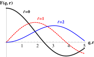
Figure 1: Beam profiles $F_{q_{r}\ell}(r)$ of the in-plane components of the vector potential (and thus of the in-plane components of the electric field) for a non-vortex beam ($\ell=0$) and TL beams ($\ell=1,2$).

Figure 1 shows the beam profile $F_{q_{r}\ell}(r)$ of the in-plane components $A_{r}$ and $A_{\varphi}$ and thus also of the in-plane components of the electric field for three different values of the OAM: $\ell=0,1,2$. In the region close to $r=0$, we observe a main difference that exists between non-vortex beams and TL. While for non-vortex beams ($\ell=0$) the amplitude has a maximum at $r=0$, for TL ($\ell\neq 0$) the amplitude of the in-plane components is zero there. Close to the origin, the profile of the in-plane components can be approximated by $F_{q_{r}\ell}(r)\propto(q_{r}r)^{|\ell|}$.

Since for Bessel functions the relation $J_{-\ell}(q_{r}r)=(-1)^{\ell}J_{\ell}(q_{r}r)$ holds, it can be seen from Eq. (9) that the structure of the beam is unchanged if simultaneously the parameters $(\sigma,\ell)$ are replaced by $(-\sigma,-\ell)$. Therefore in the following we will restrict ourselves to TL beams with $\ell>0$.

In the paraxial approximation, when $q_{r}/q_{z}\ll 1$, the $z$-component of the vector potential is disregarded. This case has been extensively used in the literature Köksal and Berakdar (2012); Babiker et al. (2002); Allen et al. (1992); Andrews (2008); Dávila Romero et al. (2002); Wätzel et al. (2012); Friese et al. (1998); Nienhuis and Visser (2004); Tabosa and Petrov (1999). The vector potential in the paraxial approximation $\mathbf{A}^{pa}(\mathbf{r},t)$ then reads

$$\mathbf{A}^{pa}(\mathbf{r},t) = A_{r}(\mathbf{r},t){\hat{\bm{r}}}+A_{\varphi}(\mathbf{r},t){\hat{\bm{\varphi}}}\,.$$ (10)

In this approximation the positive and negative frequency components of $\mathbf{A}$ are eigenstates of the angular momentum operator $-i\hbar\partial/\partial\varphi$ with eigenvalue $\hbar\ell$, which can thus be identified with the OAM per photon Andrews (2008). Although this does not strictly hold in the non-paraxial case, for the sake of brevity, in the following whenever we refer to the OAM of the beam, we are implicitly referring to the OAM of its paraxial version. The integer $\ell$ is also sometimes called the topological charge Andrews (2008).

IV A heuristic derivation of the TL-matter interaction

In this section, following the spirit of the DMA, we derive a gauge transformation that captures the essential features of TL, and at the same time retains the advantages of the DMA. The derivation is intended to be intuitive and self-evident, and is only done for the paraxial vector potential Eq. (10). A formal analysis leading to the same results will be given in Sec. VI, where the more general form of the vector potential Eq. (9) will be used and also the limitations of the paraxial approximation will be discussed.

We are interested in the interaction of TL with a planar, localized structure, such as a quantum disk or a quantum dot, whose lateral dimensions are smaller than the the characteristic radial length scale $q_{r}^{-1}$ of the beam (i.e., $q_{r}r\ll 1$). If such a structure is placed at a position with non-vanishing electric field, in particular close to the beam maximum, the conditions of the DMA are satisfied and thus the DMA is well applicable. However, this is different in the case of such a structure centered at $r=0$. At the beam center the radial profile of the vector potential can be approximated by $F_{q_{r}\ell}(r)=\alpha_{\ell}\,(q_{r}r)^{\ell}$, with $\alpha_{\ell}=A_{0}/(2^{\ell}\ell!)$. Note that the vector potential Eq. (10) and consequently also the electric field at $r=0$ are zero and thus, within the DMA there would be no interaction whatsoever.

Motivated by the EFC Hamiltonian, we try a gauge transformation function of the form

$$\chi(\mathbf{r},t) = -\frac{1}{\beta}\mathbf{r}_{\perp}\cdot\mathbf{A}^{pa}(\mathbf{r},t)\,,$$ (11)

where we have defined a two-dimensional in-plane position vector $\mathbf{r}_{\perp}=r\hat{\mathbf{r}}=x\hat{\mathbf{x}}+y\hat{\mathbf{y}}$ out of the 3D vector $\mathbf{r}$, and added a constant prefactor $1/\beta$ to be determined later. For $\beta=1$ the transformation obviously reduces to the EFC case. According to Eqs. (5) the potentials in the new gauge are calculated to

$$\mathbf{A}^{pa}\,{}^{\prime}(\mathbf{r},t)=\left(1-\frac{\ell+1}{\beta}\right)A^{pa}_{r}(\mathbf{r},t)\,\hat{\mathbf{r}}$$

$$\mbox{\quad}+\left(1-\frac{\sigma\ell+1}{\beta}\right)A^{pa}_{\varphi}(\mathbf{r},t)\,\hat{\bm{\varphi}}$$ (12a)

$$\mbox{\quad}-\frac{q_{z}}{q_{r}}\frac{q_{r}r}{\beta}F_{q_{r}\ell}(r)\sin[(\omega t-q_{z}z)-(\ell+\sigma)\varphi]\,\hat{\mathbf{z}}\,,$$

$$U^{pa}\,{}^{\prime}(\mathbf{r},t)=-\frac{1}{\beta}\mathbf{r}\cdot\mathbf{E}^{pa}(\mathbf{r},t)\,.$$ (12b)

While the radial dependence of the scalar potential as well as of the in-plane components of the new vector potential is $\sim(q_{r}r)^{\ell}$ like in the case of the old vector potential, the remaining component $A_{z}^{pa}\,{}^{\prime}$ is $\sim(q_{r}r)^{\ell+1}$ and can thus be neglected in the region close to the singularity. This is consistent with keeping terms up to order $(q_{r}r)^{\ell}$. In the EFC gauge ($\beta=1$) we then have $A_{r}^{pa}\,{}^{\prime}(\mathbf{r},t)=-\ell\mathbf{A}_{r}^{pa}(\mathbf{r},t)$ and $A_{\varphi}^{pa}\,{}^{\prime}(\mathbf{r},t)=-\sigma\ell\mathbf{A}_{\varphi}^{pa}(\mathbf{r},t)$. Thus, for $|\ell|\geq 1$ the new vector potential is not smaller than the old one clearly demonstrating that this gauge does not help to reduce the difference between mechanical and canonical momentum.

On the other hand, when $\sigma=1$ the in-plane components $A_{\varphi}^{pa}\,{}^{\prime}$ and $A_{r}^{pa}\,{}^{\prime}$ of the new vector potential vanish for $\beta=\ell+1$. As a result, $\mathbf{A}^{pa}\,{}^{\prime}(\mathbf{r},t)=0$. The Hamiltonian then reads

$$H=\frac{\mathbf{p}^{2}}{2m}+V(\mathbf{r})-\frac{{1}}{\ell+1}q\mathbf{r}_{\perp}\cdot\mathbf{E}^{pa}(\mathbf{r},t)\,.$$ (13)

We achieve a Hamiltonian which contains an EFC-like term, but with a different prefactor. Furthermore, since the new vector potential vanishes, the canonical and mechanical momenta are equal. We will refer to the transformation according to Eq. (11) with $\beta=\ell+1$ as the TL gauge. The very reason for the new prefactor $({\ell+1})^{-1}$ is the existence of a vortex, that causes the first term of an expansion of the vector potential near $\mathbf{r}=0$ to be proportional to $r^{\ell}$.

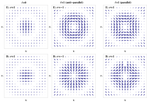
Figure 2: In-plane components of the electric and magnetic fields at $t=0$ and $z=0$ for $\ell=0$ and polarization state $\sigma=+1$ as well as for $\ell=1$, and polarization states $\sigma=-1$ (anti-parallel) and $\sigma=1$ (parallel).

For the case $\sigma=-1$, the gauge transformation with $\beta=\ell+1$ is not advantageous. This is because $A_{\varphi}^{pa}\,{}^{\prime}\neq 0$, as seen by inspecting Eq. (12), and it cannot be neglected. Conversely, choosing $\beta=-\ell+1$ (for $\ell>1$) would remove the $\varphi$-component but keep the $r$-component.

It is legitimate to wonder why there is such an asymmetry between TL fields having the same $\ell$ but differing in their circular polarization state, while an asymmetry of this type is not present in plane waves. We will further explore this in the next section.

V Electric and magnetic fields of TL

The aforementioned results suggest that there are two topologically distinct classes of TL fields, depending on the combination of OAM and circular polarization, which we will study now in detail. We calculate the electric and magnetic fields using the full form of the vector potential [Eq. (9)].

A plot of two representative cases of electric and magnetic fields for $\ell=1$ and $\sigma=\pm 1$, at $t=0$ and $z=0$ is presented in Fig. 2. For comparison, the fields of a non-vortex beam with $\ell=0$ and $\sigma=1$ are also shown. The vectorial character of the non-vortex beam is similar to a plane wave with perpendicular $\mathbf{E}$ and $\mathbf{B}$ fields. The amplitude is radially modulated according to the Bessel function $J_{0}$. In contrast, in the case of TL with $\ell=1$ the field profiles are much more complex. When $\sigma=-1$, the electric field is oriented azimuthally around the beam axis, and the magnetic field in the central region points inwards. For other values of $t$ (or $z$), the patterns change, but eventually both magnetic and electric fields cycle through the radially-like and azimuthally-like polarization patterns. In contrast, when $\sigma=1$, the fields look entirely different, and never evolve into azimuthal or radial patterns. We refer to these two as the anti-parallel [Sign$(\ell)\neq$ Sign$(\sigma)$] and the parallel [Sign$(\ell)=$ Sign$(\sigma)$] beam classes.

The field patterns shown in Fig. 2 gives an indication why a gauge, in which the scalar potential provides the dominant contribution to the coupling could be found in the parallel class but not in the anti-parallel class. In the central region the field lines of the electric field in the parallel class are similar to a vector field close to a saddle point. Such a vector field can indeed be written as the gradient of a scalar field. In contrast, in the anti-parallel class the field lines of the electric field are obviously closed indicating that this is dominantly a vortex-type field which has a non-vanishing curl and therefore cannot be obtained as a gradient of a scalar potential. Hence, in any gauge the interaction will mainly originate from the vector potential.

		Parallel	Anti-parallel
		$\ell>0,\sigma=+1$	$\ell>0,\sigma=-1$
$\mathbf{E}/(\alpha_{\ell}\omega)$	$\hat{\mathbf{r}}$	$-(q_{r}r)^{\ell}\sin[(\ell+1)\varphi]$	$-(q_{r}r)^{\ell}\sin[(\ell-1)\varphi]$
	$\hat{\bm{\varphi}}$	$-(q_{r}r)^{\ell}\cos[(\ell+1)\varphi]$	$(q_{r}r)^{\ell}\cos[(\ell-1)\varphi]$
	$\hat{\mathbf{z}}$	$\frac{1}{2(\ell+1)}\frac{q_{r}}{q_{z}}(q_{r}r)^{\ell+1}\cos[(\ell+1)\varphi]$	$-2\ell\frac{q_{r}}{q_{z}}(q_{r}r)^{\ell-1}\cos[(\ell-1)\varphi]$
$\mathbf{B}/(\alpha_{\ell}q_{z})$	$\hat{\mathbf{r}}$	$(q_{r}r)^{\ell}\left[1+\frac{q_{r}^{2}}{2q_{z}^{2}}\right]\cos[(\ell+1)\varphi]$	$-(q_{r}r)^{\ell}\left[1+(\ell-1)\frac{q_{r}^{2}}{2q_{z}^{2}}+\frac{q_{r}^{2}}{2q_{z}^{2}}\frac{4\ell(\ell-1)}{(q_{r}r)^{2}}\right]$ $\times\cos[(\ell-1)\varphi]$
	$\hat{\bm{\varphi}}$	$-(q_{r}r)^{\ell}\left[1+\frac{q_{r}^{2}}{2q_{z}^{2}}\right]\sin[(\ell+1)\varphi]$	$-(q_{r}r)^{\ell}\left[1+(\ell+1)\frac{q_{r}^{2}}{2q_{z}^{2}}-\frac{q_{r}^{2}}{2q_{z}^{2}}\frac{4\ell(\ell-1)}{(q_{r}r)^{2}}\right]$ $\times\sin[(\ell-1)\varphi]$
	$\hat{\mathbf{z}}$	$\frac{1}{2(\ell+1)}\frac{q_{r}}{q_{z}}(q_{r}r)^{\ell+1}\sin[(\ell+1)\varphi]$	$2\ell\frac{q_{r}}{q_{z}}(q_{r}r)^{\ell-1}\sin[(\ell-1)\varphi]$

Table 1: Electric and magnetic field components at $z=0$ and $t=0$ in the region close to the phase singularity calculated from the full vector potential in Eq. (9).

		Parallel	Anti-parallel
		$\ell>0,\sigma=+1$	$\ell>0,\sigma=-1$
$\mathbf{E}^{pa}/(\alpha_{\ell}\omega)$	$\hat{\mathbf{r}}$	$-(q_{r}r)^{\ell}\sin[(\ell+1)\varphi]$	$-(q_{r}r)^{\ell}\sin[(\ell-1)\varphi]$
	$\hat{\bm{\varphi}}$	$-(q_{r}r)^{\ell}\cos[(\ell+1)\varphi]$	$(q_{r}r)^{\ell}\cos[(\ell-1)\varphi]$
	$\hat{\mathbf{z}}$	0	0
$\mathbf{B}^{pa}/(\alpha_{\ell}q_{z})$	$\hat{\mathbf{r}}$	$(q_{r}r)^{\ell}\cos[(\ell+1)\varphi]$	$-(q_{r}r)^{\ell}\cos[(\ell-1)\varphi]$
	$\hat{\bm{\varphi}}$	$-(q_{r}r)^{\ell}\sin[(\ell+1)\varphi]$	$-(q_{r}r)^{\ell}\sin[(\ell-1)\varphi]$
	$\hat{\mathbf{z}}$	0	0

Table 2: Same as in Table 1, but in the paraxial approximation, i. e., obtained from Eq. (10).

It is our interest to study the region close to the phase singularity $r=0$. Thus, we provide analytical results for the field amplitudes in this region expanded in powers of $(q_{r}r)$. Table 1 presents the lowest non-vanishing orders in $(q_{r}r)$ of the electric and magnetic fields in the plane $z=0$ and at $t=0$ obtained from the full vector potential in Eq. (9). In Table 2 the same fields but obtained from the potential in the paraxial approximation [Eq. (10)] are given. Note that the in-plane vector potential of Eq. (10) gives rise to a $z$-component of the magnetic field; this component, however, has a prefactor $(q_{r}/q_{z})$ and therefore, in order to be consistent with the paraxial approximation, it has been omitted in Table 2. Indeed, it is clearly seen that if in Table 1 all terms containing a factor $(q_{r}/q_{z})$ or $(q_{r}/q_{z})^{2}$ are neglected the fields of Table 2 are obtained.

Let us first compare the full form and the paraxial case for the parallel class [Sign($\ell$)$=$Sign($\sigma$), in our case $\sigma=1$]. In the paraxial approximation we obtain pure in-plane fields with electric and magnetic fields having the same dependence on $r$. When calculated from the full vector potential, the magnetic field is slightly rescaled, the correction being of second order in the small parameter $(q_{r}/q_{z})$. Both fields acquire a small $z$-component which is of first order in $(q_{r}/q_{z})$. Additionally it is proportional to $(q_{r}r)^{\ell+1}$ and thus decreases faster for $r\to 0$ than the in-plane components. Thus, these corrections are negligible in the region close to the phase singularity and the assumptions of the paraxial approximation are well satisfied in this region.

In the anti-parallel class [Sign($\ell$) $\neq$ Sign($\sigma$), here $\sigma=-1$], on the other hand, the $z$-components of the electric and magnetic fields still contain the small parameter $(q_{r}/q_{z})$, however the radial dependence is now proportional to $(q_{r}r)^{\ell-1}$. The in-plane component of the electric field is still proportional to $(q_{r}r)^{\ell}$, thus at sufficiently small $r$ the electric field is always dominated by the $z$-component. This clearly demonstrates that the paraxial approximation, which neglects the $z$-component, is not applicable in the region close to the phase singularity. Indeed, a careful look at the $z$-component of the vector potential in Eq. (9) reveals that already there the small factor $(q_{r}/q_{z})$ is counterbalanced by a $r$-dependence which is one order lower than for the in-plane components and therefore dominates close to $r=0$.

The dominance of the $z$-component of the fields is closely related to the field profiles in the anti-parallel case shown in Fig. 2. As already mentioned, the electric field profile has a non-vanishing curl which is oriented in the $z$-direction. According to Maxwell’s equation this curl is associated with the time-derivative of a magnetic field, which therefore necessarily has to have a strong $z$-component close to $r=0$. Half an oscillation period later, the roles of electric and magnetic fields in the central column of Fig. 2 are interchanged. Then the magnetic field lines are closed circles being associated with a strong $z$-component of the electric field close to the center.

For angular momenta $\ell\geq 2$ the magnetic field in the anti-parallel class has an additional correction which is of second order in $(q_{r}/q_{z})$ but which has a $r$-dependence proportional to $(q_{r}r)^{\ell-2}$. For sufficiently small radii this is the dominant contribution to the fields. Thus, in this case close to the center the beam is dominated by the magnetic field. This holds in particular for the case $\ell=2$, in which there is a non-vanishing in-plane magnetic field at the beam center while the electric field vanishes at this point. This is again an indication that an EFC-like Hamiltonian is not applicable since with such a Hamiltonian the interaction with matter is described only in terms of the electric field.

Some research articles in the topics of highly focused TL and azimuthally/radially-polarized fields report similar findings to ours. Paraxial beams of TL can be focused using, e.g., high-NA lenses Iketaki et al. (2007); Bokor et al. (2005) or a nanoantenna Heeres et al. (2014). The theoretical analysis of focusing, based entirely on electric and magnetic fields, can be done using the formalism by Wolf Wolf (1959), and the results Iketaki et al. (2007); Bokor et al. (2005) show important similarities with the field patterns presented in Fig. 2. Azimuthally- and radially-polarized fields are a special class of TL fields Ornigotti and Aiello (2013); Volke-Sepulveda et al. (2002). The field patterns of azimuthally/radially-polarized non-paraxial Bessel beams presented by Ornigotti et al. Ornigotti and Aiello (2013) are also in agreement with our findings. Regarding the magnitude of the fields near $r=0$ Zurita-Sánchez et al. Zurita-Sánchez and Novotny (2002) have shown that, for the strongly focused azimuthally-polarized beam they studied, the magnetic interaction overcomes the electric interaction near the phase singularity; recently, their findings have been corroborated by the theoretical study of Klimov et al. Klimov et al. (2012) in the case of focused Laguerre-Gaussian beams. Finally, in their research on highly-focused TL beams, Monteiro et al. Monteiro et al. (2009), Iketaki et al. Iketaki et al. (2007) and Klimov et al. Klimov et al. (2012) report that interesting effects only occur when $\ell=1,2$ and $\sigma=-1$. The overall similarities are no coincidence, for the vector potential Eq. (9) –in contrast to Eq. (10)– shares with the aforementioned non-paraxial beams the important feature of having a non-negligible $z$-component, which we have shown to give rise to the described features.

We are now in a position to clarify the findings in the heuristic derivation of the TL-matter coupling shown in Sec. IV. There it was assumed that there is no $z$-component in the vector potential. From Table 1 we see that the $z$-component of the fields are negligible only in the parallel class. In the anti-parallel class they are proportional to $(q_{r}r)^{-1}\,F_{q_{r}\ell}(r)$. Because for $r\rightarrow 0$ the magnetic field cannot be neglected compared to the electric field, we were not able to derive an EFC-like Hamiltonian. In other words a Hamiltonian representation given solely in terms of the electric multipoles, such as $-(1/\beta)q\mathbf{r}\cdot\mathbf{E}(\mathbf{r},t)$, is insufficient to describe the TL-matter interaction for the anti-parallel class.

VI Formal derivation of the TL-matter interaction

The use of the gauge transformation function $\chi(\mathbf{r},t)$ found in Sec. IV can be motivated using formal arguments. In the following we use the more general form of Eq. (9) for the vector potential in the Coulomb gauge.

For charged particles localized around the same center, a Power-Zienau-Woolley (PZW) transformation can be done using the gauge function

$$\chi(\mathbf{r},t)=-\int_{0}^{1}\mathbf{r}\cdot\mathbf{A}(u\mathbf{r},t)du\,,$$ (14)

where $\mathbf{A}(u\mathbf{r},t)$ is given in the Coulomb gauge. This is the generalization to inhomogeneous fields of the Göppert-Mayer transformation (DMA), and leads to the so-called Poincaré gauge Cohen-Tannoudji et al. (1989); Jackson (2002). In our work we focus on the interaction of TL with planar systems. Therefore, if we consider a charge distribution mainly extended in the $x-y$ plane for a fixed $z$, the quantity $u\mathbf{r}$ scales only in the in-plane component with $u\mathbf{r}\simeq(ur,\varphi,z)$ (see, e.g., Ref. Cohen-Tannoudji et al. (1989)).

Defining $\mathbf{r}=\mathbf{r}_{\perp}+z\mathbf{\hat{z}}=r\hat{\mathbf{r}}+z\mathbf{\hat{z}}$, the gauge function reads

$$\chi(\mathbf{r},t) = -\int_{0}^{1}\mathbf{r}_{\perp}\cdot\mathbf{A}(ur,\varphi,z;t)du$$ (15)

$$-\int_{0}^{1}zA_{z}(ur,\varphi,z;t)du\,.$$

For small systems ($q_{r}r\ll 1$) the radial dependence can be approximated by $F_{q_{r}\ell}(r)\simeq\alpha_{\ell}(q_{r}r)^{|\ell|}$, which leads to $F_{q_{r}\ell}(ur)\simeq u^{|\ell|}F_{q_{r}\ell}(r)$. With these simplifications, we evaluate the integrals Eq. (15), and obtain

$$\chi(\mathbf{r},t) = -\frac{1}{|\ell|+1}\mathbf{r}_{\perp}\!\cdot\!\mathbf{A}(\mathbf{r},t)$$ (16)

$$-\frac{1}{|\ell+\sigma|+1}zA_{z}(\mathbf{r},t)\,.$$

The in-plane part of the transformation function $\chi(\mathbf{r},t)$ is exactly the same as we got in Sec. IV. In addition, there is a new term arising from the non-vanishing $z$-component of the vector potential. Note that we have neither required $\mathbf{A}^{\prime}(\mathbf{r},t)=0$ in the new gauge, nor have we neglected $A_{z}(\mathbf{r},t)$. Additionally, for non-vortex fields ($\ell=0$) with negligible $z$-component our result coincides with that of the EFC Hamiltonian.

Here we have motivated the use of Eq. (16) by showing that the TL gauge function can formally be derived by a PZW transformation for charged particles localized in a planar structure (constant $z$). Since any gauge transformation function can be postulated and used to cast the potential in suitable forms, the TL gauge can also be applied to other more general structures for variable $z$ (with varying degrees of accuracy or usefulness).

We see that the natural extension of the DMA to the case of TL beams is slightly different from the plain EFC Hamiltonian. Because of the generalized use of EFC Hamiltonians Köksal and Berakdar (2012); Al-Awfi and Babiker (2000); Babiker et al. (2002), it is worth exploring further its connection to our result. To this end, let us simply postulate a general gauge transformation of the form

$$\chi_{\beta}(\mathbf{r},t) = -\frac{1}{\beta_{r}}\mathbf{r}_{\perp}\cdot\mathbf{A}(\mathbf{r},t)-\frac{1}{\beta_{z}}zA_{z}(\mathbf{r},t)\,,$$ (17)

where $\beta_{i}$ is any number. Clearly, we can recover the TL gauge by $\beta_{r}=|\ell|+1$ and $\beta_{z}=|\ell+\sigma|+1$. In contrast, when setting $\beta_{i}=1$, Eq. (17) reduces to the EFC gauge. In the following, we will again only consider the case of $\ell>0$ and polarization $\sigma=\pm 1$, since, as already discussed, there are no essential differences in the case with negative $\ell$ and opposite sign of $\sigma$.

According to Eqs. (5b) and (17), the scalar potential in the new gauge reads

$$U^{\prime}(\mathbf{r},t) = -\frac{1}{\beta_{r}}\mathbf{r}_{\perp}\cdot\mathbf{E}(\mathbf{r},t)-\frac{1}{\beta_{z}}zE_{z}(\mathbf{r},t)\,.$$ (18)

Obviously in the scalar potential we recover an EFC-type structure of the Hamiltonian, however with in general different prefactors for the in-plane and out-of-plane components. The new vector potential in the region close to the phase singularity is given by

$${{A^{\prime}}_{r}} = \frac{{{\beta_{r}}-\left({1+\ell}\right)}}{{{\beta_{r}}}}{A_{r}}+\frac{\sigma}{{2{\beta_{z}}}}\frac{{q_{r}^{2}}}{{q_{z}^{2}}}{A_{0}}{\frac{1}{{\left({\ell+\sigma}\right)!}}}{{\left({\frac{{{q_{r}}r}}{2}}\right)}^{\ell+\sigma-1}}\left({q_{z}}z\right)$$ (19a)

$$\mbox{\qquad}\times\left[{\left({\ell+\sigma}\right)}-\frac{{\left({\ell+\sigma+2}\right)}}{{\left({\ell+\sigma+1}\right)}}{{\left({\frac{{{q_{r}}r}}{2}}\right)}^{2}}\right]\sin\left[{\left({\omega t-{q_{z}}z}\right)-\left({\ell+\sigma}\right)\varphi}\right]\,,$$

$${{A^{\prime}}_{\varphi}} = \frac{{{\beta_{r}}-\left({1+\sigma\ell}\right)}}{{{\beta_{r}}}}{A_{\varphi}}-\frac{\sigma}{{{2\beta_{z}}}}\frac{{q_{r}^{2}}}{{q_{z}^{2}}}{A_{0}}\frac{{\left({\ell+\sigma}\right)}}{{\left({\ell+\sigma}\right)!}}{{\left({\frac{{{q_{r}}r}}{2}}\right)}^{\ell+\sigma-1}}\left({q_{z}}z\right)$$ (19b)

$$\mbox{\qquad}\times\left[1-\frac{1}{{\left({\ell+\sigma+1}\right)}}{{\left({\frac{{{q_{r}}r}}{2}}\right)}^{2}}\right]\cos\left[{\left({\omega t-{q_{z}}z}\right)-\left({\ell+\sigma}\right)\varphi}\right]\,,$$

$${{A^{\prime}}_{z}} = \frac{{{\beta_{z}}-1}}{{{\beta_{z}}}}{A_{z}}-\frac{\sigma}{{{\beta_{z}}}}\frac{{{q_{r}}}}{{{q_{z}}}}{A_{0}}\frac{1}{{\left({\ell+\sigma}\right)!}}{{\left({\frac{{{q_{r}}r}}{2}}\right)}^{\ell+\sigma}}\left({q_{z}}z\right)$$ (19c)

$$\mbox{\qquad}\times\left[1-\frac{1}{{\left({\ell+\sigma+1}\right)}}{{\left({\frac{{{q_{r}}r}}{2}}\right)}^{2}}\right]\cos\left[{\left({\omega t-{q_{z}}z}\right)-\left({\ell+\sigma}\right)\varphi}\right]$$

$$-\frac{{2}}{{{\beta_{r}}}}\frac{{{q_{z}}}}{{{q_{r}}}}{A_{0}}\frac{1}{{\ell!}}{\left({\frac{{{q_{r}}r}}{2}}\right)^{\ell+1}}\sin\left[{\left({\omega t-{q_{z}}z}\right)-\left({\ell+\sigma}\right)\varphi}\right]\,,$$

where we have used the expansion in powers of $(q_{r}r)$ and kept all terms up to the order $\ell+1$.

As discussed in Sec. IV for the paraxial approximation, also here it is obvious that the EFC gauge with $\beta_{i}=1$ is not useful for TL because the transformed in-plane components of the vector potential are not smaller than the original ones. In fact, for $\ell>1$ they are in general even larger. A more detailed discussion of the EFC gauge can be found in the appendix. In the following we will restrict ourselves to the TL gauge $\beta_{r}=\ell+1$ and $\beta_{z}=\ell+\sigma+1$ and discuss the vector potential for the different cases. We remind that $A_{r}(\mathbf{r},t)$ and $A_{\varphi}(\mathbf{r},t)$ are proportional to $(q_{r}r)^{\ell}$ while $A_{z}(\mathbf{r},t)\propto(q_{r}r)^{\ell+\sigma}$.

VI.1 Vector potential in the parallel class

We first examine the new vector potential in the parallel class, i.e., Sign($\ell$) $=$ Sign($\sigma$) or, more explicitly, $\sigma=1$. The results are a direct extension to those found by the heuristic derivation in Sec. IV. In the parallel class the radial dependence of the transformed potential is the same as for the original one. Moreover, each component of the vector potential contains a term proportional to the small quantities $(q_{z}z)$. Since we assume a planar structure these terms can be neglected. Then the expressions simplify to

$$A_{r}^{\prime}(\mathbf{r},t) = 0\,,$$ (20a)

$$A_{\varphi}^{\prime}(\mathbf{r},t) = 0\,,$$ (20b)

$$A_{z}^{\prime}(\mathbf{r},t) = \left[\frac{1+\ell}{2+\ell}+2\left(\frac{q_{z}}{q_{r}}\right)^{2}\right]A_{z}(\mathbf{r},t)\,.$$ (20c)

The first thing to notice is that the components $A_{r}^{\prime}$ and $A_{\varphi}^{\prime}$ of the new vector potential are zero, as we have already found in Sec. IV. Therefore, in the Hamiltonian

$$H = \frac{{\mathbf{p}}^{2}}{2m}+V(\mathbf{r})-\frac{{1}}{\ell+1}q\mathbf{r}_{\perp}\cdot\mathbf{E}(\mathbf{r},t)-\frac{{1}}{\ell+2}qzE_{z}(\mathbf{r},t)$$ (21)

$$-\frac{{q}}{m}p_{z}A^{\prime}_{z}(\mathbf{r},t)+\frac{{q}^{2}}{2m}A^{\prime}_{z}\,{}^{2}(\mathbf{r},t)\,,$$

the in-plane TL-matter interaction can be expressed solely by a dipole-like term $-(\ell+1)^{-1}q\mathbf{r}_{\perp}\cdot\mathbf{E}(\mathbf{r},t)$ with a prefactor different to the EFC Hamiltonian. For the $z$-component we have both a dipole-like term, but also a term $-(q/m)p_{z}A^{\prime}_{z}(\mathbf{r},t)$ which still contains the vector potential. We point out that $[{q}^{2}/(2m)]A^{\prime}_{z}\,{}^{2}(\mathbf{r},t)\propto(q_{r}r)^{2\ell+2}$, and may be safely disregarded.

It is interesting to also compare again the canonical and mechanical momenta. Their difference is given by

$$\mathbf{p}-m\dot{\mathbf{r}}=qA_{z}^{\prime}(\mathbf{r},t)\,{\hat{\mathbf{z}}}\,.$$ (22)

Also here the canonical and mechanical momenta are the same for the in-plane components and only in the $z$-component a difference in the momenta arises, which is however of the order $(q_{r}r)^{\ell+1}$ and therefore one order higher than the correction to the in-plane momenta in the original gauge.

Let us now consider what happens in situations of experimental and application interest. We first address the situation when the interaction with the system only occurs through the in-plane components of the field, for example in the selective excitation of heavy holes in a quantum dot. Then, the TL-matter interaction reads $H_{\mathrm{TL-matter}}=-(\ell+1)^{-1}q\mathbf{r}_{\perp}\cdot\mathbf{E}(\mathbf{r},t)$ and is modeled by electric multipoles only with all the benefits of a DMA. Effectively we end up in the desirable situation where the vector potential is eliminated, as also shown in Sec. IV. Nevertheless the description is beyond the DMA because it keeps the full spatial dependence of the electric field and thus can give rise to transitions which are forbidden in the case of excitation by plane waves, for example transitions from envelope function with $s$-type symmetry in the valence band to those with $p$-type symmetry in the conduction band or vice versa.

Next, we consider the case where the system interacts with the $z$-component of the field, for example in intersubband transitions in quantum wells Sbierski et al. (2013) or the excitation of light holes Quinteiro et al. (2013). Here, the electric multipoles are accompanied by a magnetic term arising from the non-vanishing $z$-component of the vector potential. However, since no atypical behavior of the fields near the phase singularity occurs, it is expected that the electric interaction is larger than the magnetic one as usually happens. One could then safely only retain the electric multipolar term, and possibly neglect the difference between momenta. Therefore for the parallel class a Hamiltonian with only electric dipole-moment terms having the correct prefactors can describe the TL-matter interaction at the phase singularity.

VI.2 Vector potential in the anti-parallel class

For the anti-parallel class, we already found that a description with electric field only is not sufficient. Still, we can gain valuable insights from studying the anti-parallel case with Sign($\ell$) $\neq$ Sign($\sigma$), i.e., $\sigma=-1$. Here, the vector potential reads:

$$A_{r}^{\prime}(\mathbf{r},t) = -\frac{q_{r}^{2}}{2q_{z}^{2}}\frac{q_{z}z}{\ell}\left[(\ell+1)-\frac{4\ell(\ell-1)}{(q_{r}r)^{2}}\right]A_{\varphi}(\mathbf{r},t)\,,$$ (23a)

$$A_{\varphi}^{\prime}(\mathbf{r},t) = \frac{2\ell}{\ell+1}A_{\varphi}(\mathbf{r},t)-\frac{q_{r}^{2}}{2q_{z}^{2}}\frac{q_{z}z}{\ell}\left[(\ell-1)-\frac{4\ell(\ell-1)}{(q_{r}r)^{2}}\right]A_{r}(\mathbf{r},t)\,,$$ (23b)

$$A_{z}^{\prime}(\mathbf{r},t) = \left[\frac{\ell-1}{\ell}-\frac{2q_{z}}{q_{r}}\right]A_{z}(\mathbf{r},t)-\frac{q_{r}}{q_{z}}\frac{q_{z}z}{\ell}\left[\frac{q_{r}r}{2}-\frac{2\ell}{q_{r}r}\right]A_{r}(\mathbf{r},t)\,.$$ (23c)

Here we have kept the terms $\propto(q_{z}z)$ since, in contrast to the parallel class, they are now accompanied by radial dependencies proportional to $(q_{r}r)^{-1}$ and $(q_{r}r)^{-2}$ times the original vector potential. Thus, the transformed vector potential becomes even stronger close to the phase singularity. The magnetic interaction resulting from these terms may be comparable or even surpass the electric interaction. This is in agreement with previous results for highly focused beams, where a magnetic field contribution stronger than the electric field contribution at the phase singularity was found Zurita-Sánchez and Novotny (2002); Klimov et al. (2012). It is also interesting, that even far from the phase singularity, the in-plane term $A_{\varphi}^{\prime}$ does not vanish.

Let us study this in more detail using as an example the excitation of a quantum dot placed at the beam axis by a TL beam and energy close to the QD band-gap. Considering again the case of optical transitions with in-plane matrix elements such as the heavy hole-to-conduction band transitions, we neglect the $z$-component of the interaction, and also the terms proportional to $A^{\prime}(\mathbf{r},t)^{2}$. Then, the Hamiltonian reduces to

$$H \simeq \frac{{\mathbf{p}}^{2}}{2m}+V(\mathbf{r})-\frac{{1}}{\ell+1}q\mathbf{r}_{\perp}\cdot\mathbf{E}(\mathbf{r},t)$$ (24)

$$-\frac{{q}}{2m}\left[\mathbf{p}_{\perp}\cdot\mathbf{A}^{\prime}_{\perp}(\mathbf{r},t)+\mathbf{A}^{\prime}_{\perp}(\mathbf{r},t)\cdot\mathbf{p}_{\perp}\right]\,.$$

[We note that the angular component of the momentum vector reads $(\mathbf{p})_{\varphi}=(1/r)p_{\varphi}$, where the canonical momentum $p_{\varphi}=\partial L/\partial\dot{\varphi}$ is in fact an angular momentum Goldstein (1980).] Though there is an EFC-type Hamiltonian, clearly the in-plane vector potential remains in the Hamiltonian. We wonder how electric and magnetic contributions compare to each other. Let us specifically consider the case $\ell=2$. Then, the electric multipolar term is proportional to $r(q_{r}r)^{2}$. On the other hand, the magnetic term in Eq. (24) is proportional to $p(q_{r}r)^{0}$. If we assume that momentum and position vector are proportional to each other, as it is so in the DMA (since $\mathbf{p}=-i(m/\hbar)[\mathbf{r},H_{0}]$), it becomes clear that one should not a priori neglect the magnetic interaction, for it may be comparable or even larger the electric interaction, in particular at the phase singularity.

When the $z$-component of the fields become also important, it is clear that also here the vector potential remains in the Hamiltonian. Thus, for the anti-parallel class the TL-gauge transformation, though being mathematically correct, is in general not advantageous.

VII Conclusions

We have studied the TL-matter interaction close to the beam axis. In contrast to conventional light beams, twisted light has a phase singularity at the point $r=0$, and a strong intermixing between polarization and OAM. We distinguished the TL beams into two topologically different classes, namely the parallel class where handedness of circular polarization (i.e., the photon spin) and OAM have the same sign and the anti-parallel class where the signs of circular polarization and OAM differ.

To obtain a Hamiltonian which includes the EM fields instead of the potentials, we suggested to use a new gauge, the TL gauge. For the parallel class, the TL gauge leads to a Hamiltonian which has a dipole-type structure, but a different prefactor. For in-plane problems it takes the simple form $H_{\mathrm{TL-matter}}=-(|\ell|+1)^{-1}q\mathbf{r}_{\perp}\cdot\mathbf{E}(\mathbf{r},t)$. The prefactor is mandatory to describe the correct interaction and to achieve the identity of canonical and mechanical momentum. The origin of the prefactor in the TL gauge is the vortex, which exists at the phase singularity. For the anti-parallel class we showed that the TL gauge, which casts the Hamiltonian at least partly into electric fields, is not in general advantageous as the vector potential cannot be eliminated nor neglected. Because in the anti-parallel class magnetic effects cannot be neglected compared to the electric ones, the Hamiltonian should include magnetic as well as electric terms, and their relative strength must be analyzed in the particular problem at hand.

We compared the TL gauge to the more common DMA and EFC Hamiltonians. While for structures located close to the beam maximum the DMA is applicable, for structures located close to the beam center it cannot be used since the electric field at the phase singularity vanishes. We have also pointed out that the use of the paraxial approximation close to the phase singularity may be misleading and should be avoided at least in the anti-parallel beam class.

In contrast to other gauges the TL gauge depends explicitly on beam parameters, in particular on the OAM $\ell$. On the one hand this is clearly a restriction, but on the other hand, when TL is used to excite structures in the region of the beam center, this is usually done with the aim to address specific transitions which are driven by a light field with a given value of $\ell$. In this case a beam with a well-defined $\ell$ is used and thus, at least for beams within the parallel class, the TL gauge for this experimental set-up is well defined and can be used to write the coupling completely in terms of the electric field.

In comparison to other gauges, like the Poincaré-gauge or the multipolar gauge, the TL gauge offers the same advantages for TL beams in the parallel class as the DMA offers for slowly varying light beams: In contrast to the Poincaré-gauge, the TL gauge can be simply evaluated and leads to explicit formulas. For in-plane problems $H_{\mathrm{TL-matter}}$ contains only the electric field, which makes it manifestly gauge invariant and secures the physical meaning of the momentum operator. Furthermore, it contains all the higher order electric field couplings like coupling to quadrupole terms in a compact, appealing form.

VIII Acknowledgment

G. F. Quinteiro would like to thank P. I. Tamborenea for fruitful discussions in the topic of gauge-invariance in general and applied to TL. He also thanks the Argentine research agency CONICET for financial support through the “Programa de Becas Externas”.

Appendix A EFC gauge for twisted light

In this appendix we will discuss in some more detail why the EFC gauge is not useful for TL. We obtain the EFC gauge from our more general gauge function Eq. (17) by setting $\beta_{r}=\beta_{z}=1$. From the general formulas (19) we can then calculate the new potentials. In the parallel class, when restricting ourselves to the lowest non-vanishing order in $(q_{r}r)$ (which is the order $\ell$ for the in-plane components and $\ell+1$ for the $z$-component) and, as discussed in Sec. VI.1, neglecting terms involving the small quantities $\propto(q_{z}z)$, the expressions simplify to

$$A_{r}^{\prime}(\mathbf{r},t) = -\ell A_{r}(\mathbf{r},t)\,,$$ (25a)

$$A_{\varphi}^{\prime}(\mathbf{r},t) = -\ell A_{\varphi}(\mathbf{r},t)\,,$$ (25b)

$$A_{z}^{\prime}(\mathbf{r},t) = 2(1+\ell)\left(\frac{q_{z}}{q_{r}}\right)^{2}A_{z}(\mathbf{r},t)\,.$$ (25c)

We see that the vector potential in the EFC gauge grows with $\ell$. At first glance the Eqs. (25) might look surprising since they seem to violate the uniqueness of the EM fields: If one wanted to calculate the z-component of the magnetic field using the in-plane components of the new vector potential, one would find that $B_{z}^{\prime}=(\nabla\times\mathbf{A}^{\prime})_{z}=-\ell(\nabla\times\mathbf{A})_{z}=-\ell B_{z}$ which would violate the independence of the EM field on gauge transformations. Such a contradiction is only apparent for the following reason. We approximated the in-plane components of the vector potential to lowest order in $q_{r}r$, i.e., $(q_{r}r)^{\ell}$. Under this approximation $B_{z}=(\nabla\times\mathbf{A})_{z}=0$ and thus there is no contradiction.

The transformed vector potential also reveals a difference between canonical and mechanical momentum $\mathbf{p}-m\dot{\mathbf{r}}={q}\mathbf{A}^{\prime}(\mathbf{r},t)$, which also grows with $\ell$. Therefore, when the EFC gauge is applied to high-$\ell$ TL beams at the phase singularity and the canonical momentum instead of the mechanical momentum is used in calculations, a significant error may be introduced.

In the anti-parallel class we have

$$A_{r}^{\prime}(\mathbf{r},t)=-\ell A_{r}(\mathbf{r},t)$$

$$\mbox{\quad}-\frac{q_{r}^{2}}{2q_{z}^{2}}(q_{z}z)\left[(\ell+1)-\frac{4\ell(\ell-1)}{(q_{r}r)^{2}}\right]A_{\varphi}(\mathbf{r},t)\,,\mbox{\qquad}$$ (26a)

$$A_{\varphi}^{\prime}(\mathbf{r},t)=\ell A_{\varphi}(\mathbf{r},t)$$

$$\mbox{\quad}-\frac{q_{r}^{2}}{2q_{z}^{2}}(q_{z}z)\left[(\ell-1)-\frac{4\ell(\ell-1)}{(q_{r}r)^{2}}\right]A_{r}(\mathbf{r},t)\,,$$ (26b)

$$A_{z}^{\prime}(\mathbf{r},t)=-\frac{2q_{z}}{q_{r}}(\ell+1)A_{z}(\mathbf{r},t)$$

$$\mbox{\quad}-\frac{q_{r}}{q_{z}}(q_{z}z)\left[\frac{q_{r}r}{2}-\frac{2\ell}{q_{r}r}\right]A_{r}(\mathbf{r},t)\,.$$ (26c)

Again, the in-plane components grow with increasing $\ell$. Furthermore, like in the case of the TL gauge in the anti-parallel class (Sec. VI.2), the vector potential exhibits new terms containing $(q_{r}r)^{-n}$ multiplying the original vector potential. Thus, also in the EFC gauge the transformed vector potential becomes even stronger close to the phase singularity. For both reasons the EFC gauge is not useful in the anti-parallel class.

References

- Allen et al. (1992) L. Allen, M. W. Beijersbergen, R. J. C. Spreeuw, and J. P. Woerdman, Phys. Rev. A 45, 8185 (1992).
- Araoka et al. (2005) F. Araoka, T. Verbiest, K. Clays, and A. Persoons, Phys. Rev. A 71, 055401 (2005).
- Andrews (2008) D. L. Andrews, Structured light and its applications: An introduction to phase-structured beams and nanoscale optical forces (Academic Press, 2008).
- Padgett et al. (2004) M. Padgett, J. Courtial, and L. Allen, Physics Today 57, 35 (2004).
- Woerdemann et al. (2009) M. Woerdemann, C. Alpmann, and C. Denz, Optics Express 17, 22791 (2009).
- Dávila Romero et al. (2002) L. C. Dávila Romero, D. L. Andrews, and M. Babiker, J. Opt. B 4, S66 (2002).
- Babiker et al. (2002) M. Babiker, C. R. Bennett, D. L. Andrews, and L. C. Dávila Romero, Phys. Rev. Lett. 89, 143601 (2002).
- Quinteiro and Tamborenea (2009a) G. F. Quinteiro and P. I. Tamborenea, Europhys. Lett. 85, 47001 (2009a).
- Andersen et al. (2006) M. F. Andersen, C. Ryu, P. Cladé, V. Natarajan, A. Vaziri, K. Helmerson, and W. D. Phillips, Phys. Rev. Lett. 97, 170406 (2006).
- Simula et al. (2008) T. P. Simula, N. Nygaard, S. X. Hu, L. A. Collins, B. I. Schneider, and K. Mølmer, Phys. Rev. A 77, 015401 (2008).
- Ueno et al. (2009) Y. Ueno, Y. Toda, S. Adachi, R. Morita, and T. Tawara, Optics Express 17, 20567 (2009).
- Shigematsu et al. (2013) K. Shigematsu, Y. Toda, K. Yamane, and R. Morita, Jpn. J. Appl. Phys. 52, 08JL08 (2013).
- Wätzel et al. (2012) J. Wätzel, A. S. Moskalenko, and J. Berakdar, Optics Express 20, 27792 (2012).
- Clayburn et al. (2013) N. B. Clayburn, J. L. McCarter, J. M. Dreiling, M. Poelker, D. M. Ryan, and T. J. Gay, Phys. Rev. B 87, 035204 (2013).
- Quinteiro et al. (2010) G. F. Quinteiro, A. O. Lucero, and P. I. Tamborenea, J. Phys. Cond. Matter 22, 505802 (2010).
- Quinteiro and Tamborenea (2010) G. F. Quinteiro and P. I. Tamborenea, Phys. Rev. B 82, 125207 (2010).
- Quinteiro (2010) G. F. Quinteiro, Europhys. Lett. 91, 27002 (2010).
- Quinteiro and Tamborenea (2009b) G. F. Quinteiro and P. I. Tamborenea, Phys. Rev. B 79, 155450 (2009b).
- Quinteiro and Berakdar (2009) G. F. Quinteiro and J. Berakdar, Optics Express 17, 20465 (2009).
- Sbierski et al. (2013) B. Sbierski, G. Quinteiro, and P. Tamborenea, J. Phys. Cond. Matter 25, 385301 (2013).
- Padgett and Bowman (2011) M. Padgett and R. Bowman, Nature Photon. 5, 343 (2011).
- Quinteiro et al. (2013) G. F. Quinteiro, and T. Kuhn, Phys. Rev. B 90, 115401 (2014).
- Woerdemann et al. (2012) M. Woerdemann, C. Alpmann, M. Esseling, and C. Denz, Laser Photon. Rev. 7, 839 (2012).
- Bozinovic et al. (2013) N. Bozinovic, Y. Yue, Y. Ren, M. Tur, P. Kristensen, H. Huang, A. E. Willner, and S. Ramachandran, Science 340, 1545 (2013).
- Molina-Terriza et al. (2004) G. Molina-Terriza, A. Vaziri, J. Řeháček, Z. Hradil, and A. Zeilinger, Phys. Rev. Lett. 92, 167903 (2004).
- Molina-Terriza et al. (2007) G. Molina-Terriza, J. P. Torres, and L. Torner, Nat. Phys. 3, 305 (2007).
- D’Ambrosio et al. (2013) V. D’Ambrosio, N. Spagnolo, L. Del Re, S. Slussarenko, Y. Li, L. C. Kwek, L. Marucci, S. P. Walborn, L. Aolita, and F. Sciarrino, Nat. Commun. 4, 2432 (2013).
- Ornigotti and Aiello (2013) M. Ornigotti and A. Aiello, Optics Express 21, 15530 (2013).
- Dorn et al. (2003) R. Dorn, S. Quabis, and G. Leuchs, Phys. Rev. Lett. 91, 233901 (2003).
- Zurita-Sánchez and Novotny (2002) J. R. Zurita-Sánchez and L. Novotny, J. Opt. Soc. Am. B 19, 1355 (2002).
- Scully and Zubairy (1997) M. O. Scully and M. S. Zubairy, Quantum Optics (Cambridge University Press, Cambridge, 1997).
- Cohen-Tannoudji et al. (1989) C. Cohen-Tannoudji, J. Dupont-Roc, and G. Grynberg, Photons and Atoms: Introduction to Quantum Electrodynamics (Wiley, 1989).
- Jackson (2002) J. D. Jackson, Am. J. Phys. 70, 917 (2002).
- Bassani et al. (1977) F. Bassani, J. J. Forney, and A. A. Quattropani, Phys. Rev. Lett. 39, 1070 (1977).
- Fried (1973) Z. Fried, Phys. Rev. A 8, 2835 (1973).
- Dalgarno and Lewis (1956) A. Dalgarno and J. T. Lewis, Proc. Phys. Soc. A 69, 285 (1956).
- Dressel and Grüner (2002) M. Dressel and G. Grüner, Electrodynamics of Solids (Cambridge University Press, Cambridge, 2002).
- Barnett and Loudon (2010) S. M. Barnett and R. Loudon, Phil. Trans. R. Soc. A 368, 927 (2010).
- Herbst et al. (2003) M. Herbst, M. Glanemann, V. M. Axt, and T. Kuhn, Phys. Rev. B 67, 195305 (2003).
- Rossi and Kuhn (2002) F. Rossi and T. Kuhn, Rev. Mod. Phys. 74, 895 (2002).
- Khitrova et al. (1999) G. Khitrova, H. M. Gibbs, F. Jahnke, M. Kira, and S. W. Koch, Rev. Mod. Phys. 71, 1591 (1999).
- Reiter et al. (2006) D. Reiter, M. Glanemann, V. Axt, and T. Kuhn, Phys. Rev. B 73, 125334 (2006).
- Reiter et al. (2007) D. Reiter, M. Glanemann, V. M. Axt, and T. Kuhn, Phys. Rev. B 75, 205327 (2007).
- Lindberg et al. (1992) M. Lindberg, R. Binder, and S. Koch, Phys. Rev. A 45, 1865 (1992).
- Leitenstorfer et al. (1994) A. Leitenstorfer, A. Lohner, K. Rick, P. Leisching, T. Elsaesser, T. Kuhn, F. Rossi, W. Stolz, and K. Ploog, Phys. Rev. B 49, 16372 (1994).
- Bányai et al. (1995) L. Bányai, D. T. Thoai, E. Reitsamer, H. Haug, D. Steinbach, M. Wehner, M. Wegener, T. Marschner, and W. Stolz, Phys. Rev. Lett. 75, 2188 (1995).
- Köksal and Berakdar (2012) K. Köksal and J. Berakdar, Phys. Rev. A 86, 063812 (2012).
- Al-Awfi and Babiker (2000) S. Al-Awfi and M. Babiker, Phys. Rev. A 61, 033401 (2000).
- Klimov et al. (2012) V. V. Klimov, D. Bloch, M. Ducloy, and J. R. Leite, Phys. Rev. A 85, 053834 (2012).
- Kira et al. (1999) M. Kira, F. Jahnke, W. Hoyer, and S. W. Koch, Progr. Quantum Electron. 23, 189 (1999).
- Kobe and Smirl (1978) D. H. Kobe and A. L. Smirl, Am. J. Phys. 46, 624 (1978).
- Saleh and Teich (2007) B. E. A. Saleh and M. C. Teich, Fundamentals of of Photonics (Wiley, 2007).
- Jáuregui (2004) R. Jáuregui, Phys. Rev. A 70, 033415 (2004).
- (54) S. J. van Enk and G. Nienhuis 1994 Europhys. Lett. 25 497.
- Volke-Sepulveda et al. (2002) K. Volke-Sepulveda, V. Garcés-Chávez, S. Chávez-Cerda, J. Arlt, and K. Dholakia, J. Opt. B 4, S82 (2002).
- Friese et al. (1998) M. E. J. Friese, T. A. Nieminen, N. R. Heckenberg, and H. Rubinsztein-Dunlop, Nature 394, 348 (1998).
- Nienhuis and Visser (2004) G. Nienhuis and J. Visser, J. Opt. A 6, S248 (2004).
- Tabosa and Petrov (1999) J. W. R. Tabosa and D. V. Petrov, Phys. Rev. Lett. 83, 4967 (1999).
- Iketaki et al. (2007) Y. Iketaki, T. Watanabe, N. Bokor, and M. Fujii, Opt. Lett. 32, 2357 (2007).
- Bokor et al. (2005) N. Bokor, Y. Iketaki, T. Watanabe, and M. Fujii, Optics Express 13, 10440 (2005).
- Heeres et al. (2014) R. W. Heeres, and V. Zwiller, Nano letters 14, 4598 (2014).
- Wolf (1959) E. Wolf, Proc. Roy. Soc. London, Ser. A 253, 349 (1959).
- Monteiro et al. (2009) P. B. Monteiro, P. A. M. Neto, and H. M. Nussenzveig, Phys. Rev. A 79, 033830 (2009).
- Goldstein (1980) H. Goldstein, Classical mechanics (Addison-Wesley, second edition, 1980).