Temperature dependence of the axial magnetic effect in two-color quenched QCD

Abstract

The Axial Magnetic Effect is the generation of an equilibrium dissipationless energy flow of chiral fermions in the direction of the axial (chiral) magnetic field. At finite temperature the dissipationless energy transfer may be realized in the absence of any chemical potentials. We numerically study the temperature behavior of the Axial Magnetic Effect in quenched $SU(2)$ lattice gauge theory. We show that in the confinement (hadron) phase the effect is absent. In the deconfinement transition region the conductivity quickly increases, reaching the asymptotic $T^{2}$ behavior in a deep deconfinement (plasma) phase. Apart from an overall proportionality factor, our results qualitatively agree with theoretical predictions for the behavior of the energy flow as a function of temperature and strength of the axial magnetic field.

One of the cornerstones of modern quantum field theory is the concept of anomalies. A symmetry present at the classical level gets broken by the effects of quantum mechanics. Anomalies are responsible for quantum processes that would not occur in their absence, e.g. the decay of the neutral pion into two photons.

In the recent years it has become increasingly clear that anomalies have also important consequences in the transport properties of a gas or liquid whose constituents have chiral fermions amongst them. These effects consist of the generation of dissipationless currents in the presence of a magnetic field or a vortex. They are called the Chiral Magnetic Effect ref:CME and the Chiral Vortical Effect Erdmenger:2008rm . The currents can either be global (anomalous) currents such as the axial current or (conserved) gauge currents such as the electric current or the energy current. These transport phenomena are conveniently described by a set of transport coefficients, the chiral conductivities. They depend on the chemical potentials and the temperature. While the dependence on the chemical potentials is related to the conventional chiral anomalies the temperature dependence enters via the gravitational contribution to the anomalies Landsteiner:2011cp . On the level of Feynman diagrams the conventional anomalies appear in triangles diagrams of currents whereas the gravitational anomaly appears in triangles with one current and two energy momentum tensors.

A form of these transport laws has been derived many years ago in the context of neutrino physics Vilenkin:1979ui . Their universal character and the deeper relation to anomalies have been realized only recently. The relation to anomalies is most striking in the framework of hydrodynamics. It was shown that the hydrodynamic constitutive relations for an anomalous current necessarily have to include the chiral magnetic and chiral vortical effects and that the dependence of the chiral conductivities on the chemical potentials are completely fixed with this framework Son:2009tf . The temperature dependence is fixed via a combination of hydrodynamic and geometric reasoning Jensen:2012kj . In essence this result constitute non-renormalization theorems for the chiral conductivities.

However, in Ref. Golkar:2012kb it was shown that gauge interactions do give rise to a non-vanishing two loop contribution to the temperature dependence of the chiral conductivities. In our previous (limited) lattice study Braguta:2013loa a large suppression of the temperature dependence compared to the weak coupling result was found. Further higher loop corrections to chiral conductivities have been shown to appear in Ref. Jensen:2013vta .

In all these cases dynamical gauge fields are present. We can distinguish anomalies as “quantum” or “classical” whether the divergence of the current is given by an expression containing only classical fields or by a quantum operator. More explicitly, in the anomalous non-conservation law $\partial_{\mu}J^{\mu}=cF\tilde{F}$, $F$ might be the field strength of a purely external, non-dynamical field $A_{\mu}$ whose purpose is to act as a source for the quantum operator $J^{\mu}$ in the effective action. In this case we can speak of a c-number anomaly. The current $J$ can in this case be incorporated in a hydrodynamic formulation and the non-renormalization theorems of Son:2009tf ; Jensen:2012kj apply. If we are interested however in the axial current in QCD the field strength appearing in the anomaly equation is the gluonic one and we also need to take the quantum dynamics of the gluon fields into account. In that case the anomaly is a q-number, i.e. an operator. For the axial current in QCD it is given by the topological charge density. Now the axial charge is bound to undergo quantum fluctuations. In this case the values of the anomalous conductivities can and do suffer renormalization from interactions via dynamical gauge fields. From these considerations it becomes clear that in order to understand the role anomalous transport plays in heavy ion collisions it is of utmost importance to know how much the values of the anomalous conductivities can be modified in the strong coupling regime.

Anomalous conductivities describe the presence of dissipationless equilibrium currents. Therefore they are in principle accessible to inherently Euclidean lattice gauge theory. Most of the chiral conductivities do depend however crucially on chemical potentials whose lattice implementation is notoriously difficult. Luckily there is however one chiral conductivity that is non-vanishing even at zero chemical potential if only the system is at finite temperature. This is the chiral vortical conductivity in the axial current

$$\vec{J}_{5}=\sigma_{\mathrm{CVE},5}\,\vec{\omega}\,,$$ (1)

where $\vec{\omega}=\vec{\nabla}\times\vec{v}$ is the vorticity. This equation would still be difficult to handle on the lattice since it describes the response of the system to rotation. Another, closely related effect is the so-called Axial Magnetic Effect (AME). It describes the generation of an energy current $J^{i}_{\epsilon}=T^{0i}$ in the background of an axial magnetic field, i.e. a magnetic field that couples with opposite signs to left-handed and right-handed fermions,

$$\vec{J}_{\epsilon}=\sigma_{\mathrm{AME}}\,\vec{B}_{5}\,.$$ (2)

The Kubo formulae for these two chiral conductivities imply $\sigma_{\mathrm{CVE},5}=\sigma_{\mathrm{AME}}$. At weak coupling and for a collection of left-handed fermions with charges $q_{L}$ and right-handed fermions with charges $q_{R}$ the axial magnetic conductivity is given by

$$\sigma_{\mathrm{AME}}=\frac{1}{24}\left(\sum_{R}q_{R}-\sum_{L}q_{L}\right)T^{2}\,.$$ (3)

It is relatively simple to check the AME transport law (2) in Euclidean lattice simulations because the AME may be realized in the pure thermal vacuum with all chemical potentials set to zero, $\mu=\mu_{5}=0$. On the other hand, the lattice implementation of the axial magnetic field ${\vec{B}}_{5}$ is a straightforward procedure Braguta:2013loa ; Buividovich:2013hza .

According to Eq. (2) the axial magnetic field should induce a dissipationless energy flow of the quarks along the axis of the field. In our previous paper we have confirmed the emergence of the Axial Magnetic Effect using lattice simulations in quenched SU(2) QCD Braguta:2013loa for a certain temperature in the deconfinement phase. The same effect has been demonstrated for a system of free lattice fermions Buividovich:2013hza .

In the deconfinement phase the energy flow turned out to be proportional to the strength of the axial magnetic field in a qualitative agreement with the analytical prediction (2). Theoretically, the transport AME law (2) was derived in a linear response theory so that Eq. (2) should in principle be valid only in a weak field limit. Surprisingly, the numerical results of Ref. Braguta:2013loa have shown that the linear behavior in $B_{5}$ persists up to very high magnetic fields $eB_{5}\approx 1.2\,{\mathrm{GeV}}^{2}$. The simulations confirm with a high accuracy the linear behavior of the AME law (2) in the whole range of studied axial magnetic fields.

In the confinement phase $T<T_{c}$, and in the region close to the phase transition, $T\sim T_{c}$, the dissipationless energy transfer ceases to exist. The disappearance of the effect in the low-temperature region is a natural consequence of the fact that the AME law is essentially based on properties of the quarks, which are absent in the spectrum of the theory at low temperatures due to the quark confinement phenomenon.

In order to illustrate the existence of the effect it was sufficient to consider one fermion species, $N_{f}=1$, with a unit charge:

$$q^{L}_{5}=-q^{R}_{5}=+e\,.$$ (4)

According to Eq. (3), in QCD with two colors $N_{c}=2$ and one flavor $N_{f}=1$ the prefactor $\sigma$ in the AME law (2) has the following form:

$$\sigma^{\mathrm{th}}(T)=C^{\mathrm{th}}_{\mathrm{AME}}\,T^{2}\,,\qquad C^{\mathrm{th}}_{\mathrm{AME}}=\frac{2N_{f}N_{c}}{24}\equiv\frac{1}{6}\,.$$ (5)

The temperature behavior (5) of the conductivity coefficient $\sigma$ is assumed to be valid in a deep deconfinement phase, far from the low-temperature confining region.

In Ref. Braguta:2013loa the AME law (2) was studied numerically at the single temperature $T=480\,{\mathrm{MeV}}\simeq 1.58T_{c}$ in the deconfinement phase where $T_{c}=303\,\mathrm{MeV}$ is the critical temperature of the deconfinement phase transition of the lattice $SU(2)$ gauge theory in the continuum limit Fingberg:1992ju .

We have found that the proportionality coefficient $C_{\mathrm{AME}}$ in the AME conductivity $\sigma(T)=C_{\mathrm{AME}}\,T^{2}$ substantially differs from the theoretical prediction (5),

$$\frac{C_{\mathrm{AME}}(T)}{C^{\mathrm{th}}_{\mathrm{AME}}}{\Biggr{|}}_{T=480\,{\mathrm{MeV}}}\simeq 0.058\,.$$ (6)

The large difference between the theoretical and numerical results (6) could be a result of a peculiar temperature behavior of the proportionality coefficient $C_{\mathrm{AME}}(T)$, so that the asymptotic regime (5) may not have been reached at the studied temperature $T=480\,{\mathrm{MeV}}$.

The aim of this paper is to find the temperature behavior of the dissipationless energy transport (2) in a wide range of temperatures. In particular, we are interested in confirmation of the $T^{2}$ behavior of the proportionality coefficient predicted by the theory and verification of the validity of the theoretical prediction (5) in a deep deconfinement phase. To this end, we extend the calculations of Ref. Braguta:2013loa to a larger set of temperatures and increase statistics of numerical simulations. Below we briefly overview our numerical techniques for the sake of completeness.

We consider the following Lagrangian,

$${\cal L}_{5}={\bar{\psi}}(\partial_{\mu}-igA^{a}_{\mu}t^{a}-i\gamma^{5}eA_{5,\mu})\gamma^{\mu}\psi\equiv{\bar{\psi}}\not{{\cal D}}_{5}(A_{5})\psi\,,\quad$$ (7)

where the axial field $A_{5,\mu}$ acts as a classical background field superimposed over the dynamical non-Abelian field $A^{a}_{\mu}$ is a gauge field. In Eq. (7) $t^{a}$, $a=1,2,3$ are the generators of the corresponding $SU(2)$ gauge group. The gauge field $A^{a}_{\mu}$ is generated in lattice Monte-Carlo simulations of $SU(2)$ lattice gauge theory.

We are working in the quenched approach so that a backreaction of the fermions on the non-Abelian gauge field via the vacuum fermion loops is disregarded. It is known that the quark propagator is not strongly altered by the quenching effects ref:quenching therefore one may generally expect that the quenching should give a moderate contribution to the anomalous transport of quarks in Eq. (5). The reduced number of colors (2 instead of 3) is already taken into account in the theoretical estimate (5).

In our simulations we choose the axial gauge field in the following form

$$A_{5,0}=A_{5,3}=0,\quad A_{5,1}=-\frac{x_{2}B_{5}}{2},\quad A_{5,2}=\frac{x_{1}B_{5}}{2},\quad$$ (8)

which corresponds to a stationary uniform axial magnetic field pointing in the third direction, $B_{5,i}=B_{5}\cdot\delta_{i,3}$. Here the latin index $i=1,2,3$ labels the spatial coordinates and $\mu=0$ is the time direction. The axial electric field is absent.

According to Eq. (2) the axial magnetic background (8) should induce the dissipationless energy flow of the quarks. The latter is given by the expectation value of the $T^{0i}$ component of the stress-energy tensor,

$$J^{i}_{\epsilon} = \langle\,T^{0i}\,\rangle\equiv\frac{i}{2}\langle\,{\bar{\psi}}(\gamma^{0}{\cal D}^{i}_{5}+\gamma^{i}{\cal D}^{0}_{5})\psi\,\rangle\,.$$ (9)

In addition to the fermionic part (9), the energy flow should also contain a gluonic contribution. Although the gluons carry no electric charge, their dynamics is affected by the external magnetic field via interactions with quark vacuum loops. However, in the quenched approach the quark vacuum loops are absent so that the gluons are not sensitive to the external magnetic field. As a result the energy flow of gluons is vanishing in our approach.

The lattice implementation of the continuum formula (9) is achieved via a straightforward discretization,

$$C_{\mu}(x,y;A) = \langle\,\bar{\psi}(x)U_{x,y}(A^{a}_{\mu})\gamma_{\mu}{\psi}(y)\,\rangle_{A}$$ (10)

$$\equiv {\rm Tr}\,\left(U_{x,y}(A^{a}_{\mu})\,\frac{1}{\not{{\cal D}}_{5}+m}\,\gamma_{\mu}\right)_{x,y;A}\,,$$

where the expectation value is taken over the fermion field in a fixed background of axial $A_{5,\mu}$ and non-Abelian $A^{a}_{\mu}$ fields. These fields enter the Dirac operator ${\cal D}_{5}$ which is defined in Eq. (7). In Eq. (10) trace operation is taken over color and spinor indices, and $U_{x,y}$ is the gluon string between the lattice points $x$ and $y$ which makes Eq. (10) gauge invariant. The expectation value (10) should eventually be averaged over the ensemble of the dynamical gauge fields $A^{a}_{\mu}$.

The fermion propagator (10) is calculated using the following identity,

$${\mathrm{tr}}\left[S_{5}(A_{5})\,\gamma_{\mu}\right]\equiv{\mathrm{tr}}\left[({\cal P}_{R}+{\cal P}_{L})S_{5}(A_{5})\,\gamma_{\mu}\right]$$

$$\quad\,={\mathrm{tr}}\left[{\cal P}_{R}\,S(A_{5})\gamma_{\mu}\right]+{\mathrm{tr}}\left[{\cal P}_{L}\,S(-A_{5})\gamma_{\mu}\right],\qquad$$ (11)

where the trace is taken over spinor indices and ${\cal P}_{R,L}=(1\pm\gamma^{5})/2$ are the right and left chiral projectors, respectively. The identity (11) expresses the trace of the propagator $S_{5}(A_{5})$ in a background of the axial field $A_{5}$ via the traces of the usual propagators $S({\cal A})$ calculated in the background of the standard $U(1)$ gauge fields ${\cal A}$,

$$S_{5}(A_{5})=\left[\not{{\cal D}}_{5}(A_{5})\right]^{-1},\qquad S({\cal A}) = \left[\not{{\cal D}}({\cal A})\right]^{-1}.$$ (12)

The Dirac operator for the former is defined in Eq. (7) while the one for the latter has the usual form:

$${\cal D}_{\mu}({\cal A})=\partial_{\mu}-igA^{a}_{\mu}t^{a}-ie{\cal A}_{\mu}\,.$$ (13)

In Eq. (11) the axial gauge field $A_{5}$ appears as the Abelian field coupled with opposite signs to right-handed and left-handed fermions, in agreement with the prescription for the left- and right-handed charges (4).

The correlation functions (10) are calculated according to the numerical setup of Refs. Buividovich:2009wi . The quark fields are simulated with the help of the overlap lattice Dirac operator $\mathcal{D}$ with exact chiral symmetry Neuberger:98:1 . The discretized version of Eq. (9) is calculated using the correlation functions (10), which are averaged over an equilibrium finite-temperature ensemble of non-Abelian gauge field configurations ${\cal A}_{\mu}$:

$$\left\langle{\cal O}\right\rangle=\left(\int DA^{a}_{\mu}\,e^{-S_{YM}[A^{a}_{\mu}]}\right)^{\hskip-1.42262pt-1}\hskip-4.2679pt\int DA^{a}_{\mu}\,e^{-S_{\mathrm{YM}}[A^{a}_{\mu}]}\,{\cal O}\,,\quad$$

where $S_{\mathrm{YM}}(A^{a}_{\mu})$ is the Yang-Mills lattice action.

We evaluate the energy flow (9) using 2700 gauge configurations for every value of parameters (spatial $L_{s}$ and temporal $L_{t}$ lattice sizes, lattice spacing $a$ and strength of the axial gauge field $eB_{5}$). In our previous simulations Braguta:2013loa – which were carried out with much smaller statistics – we have consider the asymmetric lattices $L_{s}^{3}L_{t}$ with three temporal lengths $L_{t}=4,6,8$ and the fixed spatial length $L_{s}=14$. In addition, we have checked the robustness of the results with respect to variations of the volume and the lattice spacing.

In this paper we explore the high-temperature part of the phase diagram concentrating on single value of the temporal lattice extension $L_{t}=4$ and larger spatial lattice volumes $L_{s}=16,\,18,\,20$. We make our simulations for the physical lattice spacings in the interval $a=(0.068\dots 0.148)$ fm and the temperature range $T=(330\dots 720)\,{\mathrm{MeV}}$.

We use the improved lattice action for the gluon fields Bornyakov:2005iy . Due to the identity (11), the axial magnetic field shares many properties of the usual magnetic field. For example, the strength of the axial magnetic field is subjected to quantization due to the periodicity of the gauge fields in a finite lattice volume:

$$B_{5}=k\,B_{5,\mathrm{min}}\,,\qquad eB_{5,\mathrm{min}}=\frac{2\pi}{L^{2}_{s}}\,.\qquad$$ (14)

Here the integer number $k=0,1,\dots,L_{s}^{2}/2$ determines the total number of elementary magnetic fluxes threading each $(x^{1},x^{2})$ plane of the lattice. The quantization (14) is consistent with the unit charges of the left- and right-handed quarks (4). In order to avoid ultraviolet artifacts, we simulate the lattice at relatively small values of the flux quanta $k\leq 15$ which is much smaller than the maximal possible value of the quantized flux, $k_{\mathrm{max}}=L^{2}_{s}/2\sim 100$. Our typical strongest magnetic fields are of the order $eB_{5,\mathrm{max}}\sim 1.\,{\mathrm{GeV}}^{2}$ while the smallest possible fields are of the order of $eB_{5,\mathrm{min}}\sim 0.1\,{\mathrm{GeV}}^{2}$.

We have numerically checked that the dissipationless energy flow scales linearly with the strength of the axial magnetic field $B_{5}$ for a wide set of temperature and volumes, in agreement with the theoretical prediction (2) and our previous numerical calculations Braguta:2013loa . Thus, in order to find the temperature behavior of the conductivity coefficient,

$$C_{\mathrm{AME}}(T)=\frac{J_{\epsilon}(T,eB_{5})}{eB_{5}T^{2}}\,,$$ (15)

it is sufficient to calculate the energy current $J_{\epsilon}$ for a single value of the external axial magnetic field $B_{5}$ at a given temperature $T$.

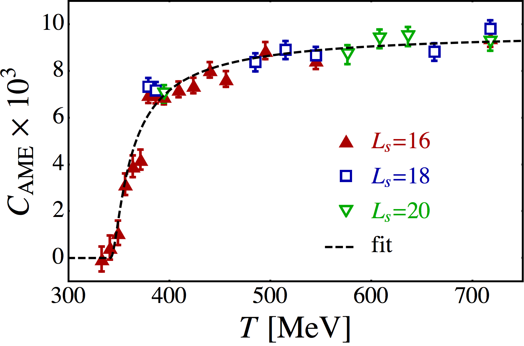
Figure 1: The dimensionless conductivity coefficient (15) of the dissipationless energy flow vs. temperature. The dashed line represents the best fit by Eq. (16).

In Fig. 1 we show the dimensionless coefficient (15) of the conductivity (3) as a function of temperature $T$. In agreement with our previous results Braguta:2013loa , the dissipationless energy transfer is absent in the confinement phase. The conductivity coefficient $C_{\mathrm{AME}}(T)$ raises with temperature at phase transition region, and approaches a constant value at $T\sim 500\,{\mathrm{MeV}}$ [$T\sim 1.5\,T_{c}$ for the SU(2) gauge theory] implying the $T^{2}$ behavior of the conductivity $\sigma(T)$ at higher temperatures.

We find the the temperature behavior of the coefficient $C_{\mathrm{AME}}$ can well be described by the following function,

$$C^{\mathrm{fit}}_{\mathrm{AME}}(T)=C^{\infty}_{\mathrm{AME}}\,\exp\left(-\frac{h\,T_{0}}{T-T_{0}}\right)\,,\quad T>T_{0}\,,\quad$$ (16)

with the best fit parameters

$$C_{\mathrm{AME}}^{\infty}=0.0097(2)\,,$$ (17)

$h=0.055(7)$ and $T_{0}=339(2)\,{\mathrm{MeV}}$. The best fit value for the temperature scale is quite close to the pseudocritical temperature of the deconfinement transition of the lattice $SU(2)$ gauge theory at our lattices. The quality of the fit (16) is given by $\chi/{\mathrm{d.o.f.}}=1.8$. The fit is shown in Fig. 1 by the dashed line.

The quantity (17) corresponds to the AME conductivity $\sigma(T)=C_{\mathrm{AME}}^{\infty}\,T^{2}$ in the high-temperature limit. For a conformal theory with two colors of fermions and one single flavor, the theoretical proportionality coefficient should be an order of magnitude larger (5), $C^{\mathrm{th}}_{\mathrm{AME}}=1/6\approx 0.166$. The ratio between the observed and predicted coefficients is the same as in our previous study (6). Notice that in lattice simulations of free fermions the anomalous energy flow agrees very well with the theoretical predictions Buividovich:2013hza while we observe a large discrepancy between theoretical and numerical results in the lattice simulations of the interacting gauge theory.

Figure 1 also demonstrates the robustness of the result with respect to variations of the lattice volume. For example, the results at $T\approx 400\,{\mathrm{MeV}}\approx 1.3\,T_{c}$) and $T\approx 720\,{\mathrm{MeV}}\approx 2.37\,T_{c}$ stay unchanged within the error bars as the volume changes in the range $V=(8\dots 15)\,{\mathrm{fm}}^{3}$ and $V=(1.3\dots 2.6)\,{\mathrm{fm}}^{3}$, respectively. This behavior is contrasted with the simulations of the same effect in a theory with free fermions, where large finite-volume corrections were observed Buividovich:2013hza . The energy flow is almost insensitive to variations of the ultraviolet cutoff given by inverse lattice spacing Braguta:2013loa .

Concluding, we have numerically calculated the temperature behavior of the dissipationless energy flow induced by the background axial magnetic field (the Axial Magnetic Effect) in the quenched lattice $SU(2)$ gauge theory. We show that the energy flow is absent in the confinement phase. In the deconfinement phase the conductivity flow is proportional to the strength of the axial magnetic field. The AME conductivity raises sharply in the phase transition region at $T\sim T_{c}$ and reaches the expected $T^{2}$ behavior as the temperature increases over $1.5\,T_{c}$. However, the numerically found conductivity coefficient is approximately 17 times smaller than the coefficient predicted by the linear response theory at weak coupling.

- (1) K. Fukushima, D. E. Kharzeev and H. J. Warringa, Phys. Rev. D 78, 074033 (2008); D. E. Kharzeev, L. D. McLerran and H. J. Warringa, Nucl. Phys. A 803, 227 (2008); A. Vilenkin, Phys. Rev. D 22, 3080 (1980); M. A. Metlitski and A. R. Zhitnitsky, Phys. Rev. D 72, 045011 (2005). M. Giovannini and M. E. Shaposhnikov, Phys. Rev. D 57, 2186 (1998); A. Y. Alekseev, V. V. Cheianov and J. Frohlich, Phys. Rev. Lett. 81, 3503 (1998).
- (2) J. Erdmenger, M. Haack, M. Kaminski and A. Yarom, JHEP 0901 (2009) 055; N. Banerjee, J. Bhattacharya, S. Bhattacharyya, S. Dutta, R. Loganayagam and P. Surowka, JHEP 1101 (2011) 094. D. T. Son and A. R. Zhitnitsky, Phys. Rev. D 70, 074018 (2004).
- (3) K. Landsteiner, E. Megias and F. Pena-Benitez, Phys. Rev. Lett. 107, 021601 (2011) and Lect. Notes Phys. 871 (2013) 433 [arXiv:1207.5808 [hep-th]]. K. Landsteiner, E. Megias, L. Melgar and F. Pena-Benitez, JHEP 1109 (2011) 121.
- (4) A. Vilenkin, Phys. Rev. D 20 (1979) 1807; A. Vilenkin, Phys. Rev. D 21 (1980) 2260.
- (5) D. T. Son and P. Surowka, Phys. Rev. Lett. 103 (2009) 191601; Y. Neiman and Y. Oz, JHEP 1103 (2011) 023; A. V. Sadofyev, V. I. Shevchenko, and V. I. Zakharov, Phys. Rev. D 83, 105025 (2011); V. P. Nair, R. Ray and S. Roy, Phys. Rev. D 86, 025012 (2012); V. I. Zakharov, Lect. Notes Phys. 871, 295 (2013) [arXiv:1210.2186 [hep-ph]].
- (6) K. Jensen, R. Loganayagam and A. Yarom, JHEP 1302, 088 (2013).
- (7) S. Golkar and D. T. Son, arXiv:1207.5806 [hep-th]; D. -F. Hou, H. Liu and H. -c. Ren, Phys. Rev. D 86 (2012) 121703.
- (8) V. Braguta, M. N. Chernodub, K. Landsteiner, M. I. Polikarpov and M. V. Ulybyshev, Phys. Rev. D 88, 071501 (2013).
- (9) K. Jensen, P. Kovtun and A. Ritz, JHEP 1310, 186 (2013); E. V. Gorbar, V. A. Miransky, I. A. Shovkovy and X. Wang, Phys. Rev. D 88, 025025 (2013).
- (10) P. V. Buividovich, arXiv:1312.1843 [hep-lat]; arXiv:1309.4966 [hep-lat].
- (11) J. Fingberg, U. M. Heller and F. Karsch, Nucl. Phys. B 392, 493 (1993).
- (12) P. O. Bowman, U. M. Heller, D. B. Leinweber, M. B. Parappilly, A. G. Williams, J. Zhang, Phys. Rev. D 71, 054507 (2005).
- (13) P. V. Buividovich, M. N. Chernodub, E. V. Luschevskaya and M. I. Polikarpov, Phys. Rev. D 80, 054503 (2009); P. V. Buividovich, M. N. Chernodub, D. E. Kharzeev, T. Kalaydzhyan, E. V. Luschevskaya and M. I. Polikarpov, Phys. Rev. Lett. 105, 132001 (2010).
- (14) H. Neuberger, Phys. Lett. B 417, 141 (1998).
- (15) V. G. Bornyakov, E. M. Ilgenfritz, M. Muller-Preussker, Phys. Rev. D 72 (2005) 054511; V. G. Bornyakov, E.-M. Ilgenfritz, B. V. Martemyanov, S. M. Morozov, M. Muller-Preussker and A. I. Veselov, Phys. Rev. D 76, 054505 (2007).