High order solution of Poisson problems with piecewise constant coefficients and interface jumps

Abstract

We present a fast and accurate algorithm to solve Poisson problems in complex geometries, using regular Cartesian grids. We consider a variety of configurations, including Poisson problems with interfaces across which the solution is discontinuous (of the type arising in multi-fluid flows). The algorithm is based on a combination of the Correction Function Method (CFM) and Boundary Integral Methods (BIM). Interface and boundary conditions can be treated in a fast and accurate manner using boundary integral equations, and the associated BIM. Unfortunately, BIM can be costly when the solution is needed everywhere in a grid, e.g. fluid flow problems. We use the CFM to circumvent this issue. The solution from the BIM is used to rewrite the problem as a series of Poisson problems in rectangular domains — which requires the BIM solution at interfaces/boundaries only. These Poisson problems involve discontinuities at interfaces, of the type that the CFM can handle. Hence we use the CFM to solve them (to high order of accuracy) with finite differences and a Fast Fourier Transform based fast Poisson solver. We present 2-D examples of the algorithm applied to Poisson problems involving complex geometries, including cases in which the solution is discontinuous. We show that the algorithm produces solutions that converge with either 3${}^{\textrm{rd}}$ or 4${}^{\textrm{th}}$ order of accuracy, depending on the type of boundary condition and solution discontinuity.

1 Introduction.

In this paper we present a fast and accurate numerical algorithm to solve Poisson problems in complex geometries, using regular Cartesian grids. It can be applied to a wide variety of Poisson problems, particularly those with interfaces across which jump conditions are prescribed for both the solution and its weighted normal derivatives. The solution to problems of this type is of fundamental importance in, for example, the description of fluid flows separated by interfaces (e.g. the interfaces between immiscible fluids, or fluids separated by a membrane). The algorithm is based on the combination of the Correction Function Method (CFM) [1] and boundary integral formulations of the Laplace equation [2, 3, 4].

Standard finite differences discretizations cannot be directly used in the vicinity of a discontinuity interface. There is a variety of algorithms that have been proposed for dealing with problems of this type (a brief review of the literature is included below). In this paper we will employ the CFM. The CFM produces accurate solutions by introducing smooth extensions (via the correction function), across the interface, of the solution on each side. These extensions are then used to complete the finite differences stencils straddling the interface. This produces corrections which affect only the right hand side of the linear system that would have resulted in the problem without the interface. The idea is similar to the one used by the Immersed Boundary Method [5], the Immersed Interface Method [6], and the Ghost Fluid Method [7]. The difference is that in the CFM the corrections are not computed using expansions. Instead, the correction function is used, which is defined as the solution to a PDE, and can be separately solved with any desired accuracy. As discussed in [1], the CFM can be employed to solve the Poisson equation with an arbitrary immersed interface, across which the solution obeys appropriate jump conditions, in a regular Cartesian grid.

However, the CFM [1] imposes restrictions on the type of interface jump conditions that it allows, which are not (generally) satisfied by the problems that arise in applications. In this paper we show how to remove these restrictions. To do so we build on an idea introduced by Mayo [8] to replace the original problem by sub-problems, each of which can be solved with the CFM. A brief summary of the process, described in detail in §4, follows.

We write the solution as the sum of two components. The first component satisfies the Poisson problem in which the jump in the normal derivative across the interface is set to vanish. By construction this first problem can be solved using the CFM. The second component solves the “deficit” problem, a Laplace equation which takes care of the jumps in the normal derivatives at the interface. This second problem can be solved using a boundary integral method (BIM) [2, 8, 3]. However, we do not use the BIM to compute the solution at every grid point, as this would be too costly. Instead we use the potential densities (at the interface) from the BIM, to write a third problem which the second component satisfies, which can be efficiently solved with the CFM.

Furthermore, in the steps where the CFM is used, the solution domain is embedded into a rectangular box. As a consequence, the linear algebraic systems that a finite differences discretization and the CFM produce, can be efficiently solved using Fast Fourier transform (FFT) techniques . Effectively, the problem is reduced to: (i) solving two standard (no interfaces, which are removed by the CFM formulation) Poisson problems in a box, with Dirichlet boundary conditions at the box boundary, and (ii) using a BIM to compute potential densities at the interfaces and the boundary. The overall solution procedure is fast: the costliest steps involve fast solutions of boundary integral equations [9, 10, 11], and an FFT-based fast Poisson solver.

Finally, in principle the BIM and the CFM can be implemented to any order of accuracy. Therefore, the present algorithm can be made as accurate as one desires.

There exists a vast literature on immersed methods for the Poisson equation and related problems. By immersed methods here we mean: methods where the entire solution domain (normally involving complex geometries) is immersed into a regular Cartesian grid or triangulation. In particular, the combination of boundary integral equations and immersed methods was introduced in the seminal work by Mayo and co-authors [8, 12, 13]. Recent work of particular interest focuses on Kernel-Free Boundary Integral Methods [14]. This new class may offer better efficiency for 3-D problems. Some of the other well established methods include the work by Johansen and Collela [15], the Immersed Boundary Method [5, 16, 17], the Immersed Interface Method [6, 18, 19, 20, 21, 22], the Ghost Fluid Method [7, 23, 24, 25, 26, 27], and the Immersed Boundary Smooth Extension Method [28]. A recent development is the Voronoi Interface Method [29], an extension of the Ghost Fluid Method that achieves second accuracy in the solution and first order accuracy in the gradient for all regimes. The finite element community has also made significant progress in developing new immersed methods. For example, the work by Dolbow and Harari [30], the Extended Finite Element Method [31], the Virtual Node Method [32], the finite element versions of the Immersed Interface Method [33, 34, 35, 36], and the Exact Subgrid Interface Correction Method [37].

High order (specifically fourth order) implementations of some the methods mentioned above are known. For example: Ghost Fluid Method [38], and combination of BIM and immersed methods [39, 40].

The present paper is inspired by the work by Mayo and co-authors [8, 12, 13]. We extend some of their general ideas by incorporating the CFM, which allows us to solve Poisson problems involving interface jumps, and offers a general framework to develop high order schemes.

The remainder of the paper is organized as follows. In §2 we introduce the general Poisson problem that we seek to solve. In §3 we review well established results pertaining to the potential formulation of the Laplace equation. In §4 we present the proposed algorithm, and discuss details such as accuracy and computational cost. In §5 we show examples of the algorithm applied to problems involving complex geometries and interfaces of discontinuity, including convergence results. Finally, §6 contains the conclusions.

2 Definition of the problem

2.1 Notation

Throughout this paper, $\vec{x}=(x_{1}\/,\,x_{2}\/,\,\dots)\in\mathbb{R}^{\nu}\/$ is the spatial vector (where $\nu=2\/$ or $\nu=3\/$), $\Delta\/$ is the Laplace operator defined by

$$\Delta\/=\sum_{i=1}^{\nu}\dfrac{\partial^{2}}{\partial x_{i}^{2}}\/,$$ (1)

and $\Omega\/$ is an arbitrary, bounded and open, simply connected domain in $\mathbb{R}^{\nu}\/$, with a piece-wise smooth boundary $\partial\Omega\/$. This domain is split into two sub-domains by a co-dimension 1 surface $\Gamma\/$ disjoint from the boundary $\partial\Omega\/$. We denote the sub-domain interior to $\Gamma\/$ by $\Omega^{-}\/$, and the sub-domain exterior to $\Gamma\/$ by $\Omega^{+}\/$. The situation we have in mind is best described by a picture: see figure 1.

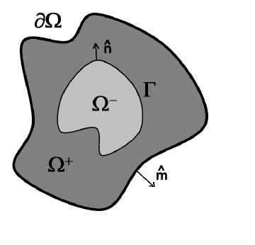
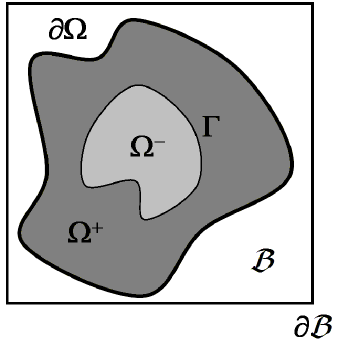
Figure 1: Left: typical solution domain $\Omega\/$, split by an internal interface $\Gamma\/$ across which the solution and the equation coefficients jump. Note that there is no problem with allowing $\Omega^{-}\/$ to have more than one component. Right: the box $\mathcal{B}$ enclosing $\Omega\/$. The role of $\mathcal{B}$ is explained in §4.

Let $\hat{n}\/$ denote the unit vector normal to $\Gamma\/$, pointing towards $\Omega^{+}\/$, and let $u\/$ be a function defined in a neighborhood of $\Gamma\/$. Then

$$u_{n} =\hat{n}\cdot\vec{\nabla}u=\hat{n}\cdot(u_{x_{1}}\/,\,u_{x_{2}}\/,\,\dots) \mbox{for}\;\vec{x} \in\Gamma$$ (2)

denotes the derivative of $u\/$ in the direction of $\hat{n}\/$. Similarly, $\hat{m}\/$ and $u_{m}\/$ denote the outer normal vector to the boundary $\partial\Omega\/$, and the corresponding directional derivative.

Furthermore, we are interested in problems that involve jumps. Let $\vec{x}=\vec{x}_{0}+\epsilon\hat{n}(\vec{x}_{0})\/$, where $\vec{x}_{0}\in\Gamma\/$. Then, we denote jumps across the surface $\Gamma\/$ at $\vec{x}_{0}\/$ by

$$[u(\vec{x}_{0})]_{\Gamma}=\lim_{\epsilon\uparrow 0}u(\vec{x})-\lim_{\epsilon\downarrow 0}u(\vec{x})\/,$$ (3)

and the corresponding mean value by

$$\langle u(\vec{x}_{0})\rangle_{\Gamma}=\dfrac{1}{2}\lim_{\epsilon\uparrow 0}u(\vec{x})+\dfrac{1}{2}\lim_{\epsilon\downarrow 0}u(\vec{x})\/.$$ (4)

Similar expressions apply to jumps across $\partial\Omega\/$.

2.2 Poisson problems with an interface

Our objective is to solve Poisson problems of the form:

$$\vec{\nabla}\cdot(\beta\/^{+}\vec{\nabla}u(\vec{x})) =f^{+}(\vec{x}) \mathrm{for}\;\;\vec{x} \in\Omega\/^{+},$$ (5a)

$$\rule{0.0pt}{11.99998pt}\vec{\nabla}\cdot(\beta\/^{-}\vec{\nabla}u(\vec{x})) =f^{-}(\vec{x}) \mathrm{for}\;\;\vec{x} \in\Omega\/^{-},$$ (5b)

with the jump conditions

$$[u(\vec{x})]_{\Gamma} =a(\vec{x}) \mathrm{for}\;\;\vec{x} \in\Gamma\/,$$ (6a)

$$\rule{0.0pt}{11.99998pt}\bigl{[}\beta\/u_{n}(\vec{x})\bigr{]}_{\Gamma} =b(\vec{x}) \mathrm{for}\;\;\vec{x} \in\Gamma\/,$$ (6b)

and either Dirichlet or Neumann boundary conditions:

$$u(\vec{x}) =g_{D}(\vec{x}) \mathrm{for}\;\;\vec{x} \in\partial\Omega\/,$$ (7a)

$$\rule{0.0pt}{11.99998pt}\mathrm{or}\qquad u_{m}(\vec{x}) =g_{N}(\vec{x}) \mathrm{for}\;\;\vec{x} \in\partial\Omega\/.$$ (7b)

Here $\beta^{\pm}\/$ are positive constants, $f^{\pm}\colon\Omega^{\pm}\mapsto\mathbb{R}\/$, $a\/$, $b\colon\Gamma\mapsto\mathbb{R}$, and $g_{D}\/$, $g_{N}\colon\partial\Omega\mapsto\mathbb{R}$ are some given functions.  Furthermore, in the case of Neumann boundary condition, equation (7b), we further assume that the following compatibility condition is satisfied

$$\int_{\Omega}f\,d\/V=\int_{\partial\Omega}\beta^{+}g_{N}\,d\/S-\int_{\Gamma}b\,d\/S\/.$$ (8)

In the development of the algorithm, it is convenient to rewrite (6b) in terms of $[u_{n}]_{\Gamma}\/$. We use the following identity

$$[pq]=\langle p\rangle[q]+[p]\langle q\rangle,$$ (9)

to write the alternative form

$$[u_{n}]_{\Gamma}+\lambda\langle u_{n}\rangle_{\Gamma} =b(\vec{x})/\langle\/\beta\/\rangle_{\Gamma}\/.$$ (10)

where $\lambda=[\beta]_{\Gamma}/\langle\beta\rangle_{\Gamma}\/$.

The problems above are known as interior Poisson problems [3] because we solve for $u\/$ in the interior of the boundary $\partial\Omega\/$. In contrast, in exterior Poisson problems we solve for $u\/$ in the exterior of $\partial\Omega\/$. Exterior problems can be solved with techniques analogous to the ones used in this paper, but we will not consider them in here.

We also discuss the solution to open space problems, where the solution is defined everywhere, i.e. $\Omega=\mathbb{R}^{\nu}\/$. In this case, we assume that $f\/$ is compact support and denote the support of $f\/$ by $\Omega_{f}\/$. Furthermore, to guarantee uniqueness, we also assume that the solution exhibits the following asymptotic behavior

$$u(\vec{x}) \;\sim\;\dfrac{F}{2\pi}\ln\lvert\vec{x}\rvert, \lvert\vec{x}\rvert\gg 1 \nu=2$$ for and , (11a)

$$u(\vec{x}) \;\sim\;\dfrac{F}{(\nu-2)A_{\nu}\lvert\vec{x}\rvert^{\nu-2}}, \lvert\vec{x}\rvert\gg 1 \nu=3$$ for and , (11b)

where $A_{\nu}\/$ is area of the unit sphere in $\mathbb{R}^{\nu}\/$, and

$$F=\dfrac{1}{\beta^{+}}\int_{\Omega^{+}}f^{+}\,d\/V+\dfrac{1}{\beta^{-}}\int_{\Omega^{-}}f^{-}\,d\/V+\int_{\Gamma}[u_{n}]_{\Gamma}dS\/.$$ (12)

Remark 1.

In the literature the case when $\beta^{+}=\beta^{-}\/$ is often called the constant coefficients case, while $\beta^{+}\neq\beta^{-}\/$ is referred to as the discontinuous coefficients case. There is also the case where $\beta^{\pm}=\beta^{\pm}(\vec{x})\/$, known as variable coefficients case. This last case is not treated in this paper.  $\clubsuit\/$

Remark 2.

The solution to (5–6) with Neumann boundary condition (7b) (interior Neumann problem) is defined up to an arbitrary additive constant. There is a number of techniques that can be used to obtain a solution to this problem [8, 3, 41]. In §4.6 we discuss how we use the Generalized Minimum Residual Method (GMRES) [42] to obtain accurate solutions to the singular systems of equations that arise in this context.  $\clubsuit\/$

2.3 The large $\beta\/$ ratio limit

Many applications in multiphase flows involve the solution of problems like the ones above, with a large ratio between the coefficients $\beta^{\pm}\/$. For example, in the simulation of multi-phase flows, $\beta\/$ is the reciprocal of the fluid density, and hence for air-water interfaces the ratio of $\beta^{\pm}\/$ is $10^{3}\/$. As we will demonstrate, the solution algorithm presented in §4 is general enough to deal with such ratios, and larger.

However, the situation where $\beta^{-}/\beta^{+}\gg 1\/$ involves a subtlety. In the limit $\beta^{-}/\beta^{+}\to\infty\/$, equation (10) yields $u^{-}_{n}=0\/$, where $u^{-}\/$ denotes the restriction of $u\/$ to $\Omega^{-}\/$. Thus $u^{-}\/$ becomes the solution to a Poisson problem, with a Neumann boundary condition on $\Gamma=\partial\Omega^{-}\/$. Hence $u^{-}\/$ is defined only up to an arbitrary additive constant. For this reason, when $\beta^{-}/\beta^{+}\/$ is large, the Poisson problem in (5–6) becomes poorly conditioned. This issue is intrinsic to the problem being solved, independent of the numerical algorithm used.

In §4.7 we discuss an approach to to remove the poor conditioning in the context of the algorithm described here.

3 Potential formulation

In this section we review a few basic results pertaining to the fundamental solution of the Laplace equation, as they will be important to design our method. A detailed discussion of these results are found in many textbooks on the subject, e.g. [3, 43, 4].

Let $\Phi=\Phi(\vec{x}\/,\,\vec{y})\/$ denote the fundamental solution of the Laplace equation, defined by

$$\Delta\,\Phi=\delta(\vec{x}-\vec{y})\/,$$ (13)

where $\delta\/$ denotes the Dirac delta distribution. In particular

• in 2-D,

  ${\displaystyle\Phi=\dfrac{1}{2\,\pi}\,\ln(\lvert\vec{x}-\vec{y}\rvert)}\/$,

• in 3-D,

  ${\displaystyle\Phi=-\dfrac{1}{4\,\pi\,\lvert\vec{x}-\vec{y}\rvert}}\/$,

• generally, in $\nu\geq 3\/$ dimensions,

  ${\displaystyle\Phi=-\dfrac{1}{(\nu-2)\,A_{\nu}\,\lvert\vec{x}-\vec{y}\rvert^{\nu-2}}}\/$,
  where $A_{\nu}=\/$ area of the unit sphere in $\mathbb{R}^{\nu}\/$.

For $\vec{x}\in\Gamma\/$ (or $\vec{x}\in\partial\Omega\/$), $\Phi_{n}\/$ (or $\Phi_{m}\/$) denotes the normal derivative of $\Phi(\vec{x}\/,\,\vec{y})\/$ with respect to $\vec{x}\/$. Furthermore, for $\vec{x}\in\Gamma\/$ and $\vec{y}\in\partial\Omega\/$, $\Phi_{n\/m}\/$ is the object:

$$\Phi_{n\/m}=\sum_{i\,j}n_{i}\,m_{j}\,\dfrac{\partial^{2}}{\partial x_{i}\,\partial y_{j}}\,\Phi\/.$$ (14)

Fairly straightforward, but tedious, calculations show that the singularity in $\Phi\/$ is such that

For $$\vec{x}\in\Gamma\/ \Phi\/ \Phi_{n}\/ \vec{y}\/ \Gamma\/$$, and are integrable as functions of in . (15)

Many common boundary integral formulations of the Laplace equation follow from Green’s third identity [4]. This identity shows that the solution to the Laplace equation can be written as a combination of single and double layer potentials. For ease of presentation, here we describe single and double layer potentials based on $\Gamma\/$, but similar results apply to $\partial\Omega\/$.

A single layer potential solution based on $\Gamma\/$ has the form

$$u^{\text{SL}}(\vec{x})=\int_{\Gamma}\rho(\vec{y})\Phi(\vec{x}\/,\,\vec{y})\,d\/S\/,$$ (16)

where the integration is taken over $\vec{y}\in\Gamma\/$, and $\rho\/$ is the single layer density defined over $\Gamma\/$. A single layer potential is a solution of the Laplace equation everywhere in $\mathbb{R}^{\nu}\/$, and it satisfies the following jump conditions

$$[u^{\text{SL}}(\vec{x})]_{\Gamma} =0\/,$$ (17a)

$$\rule{0.0pt}{11.99998pt}[u^{\text{SL}}_{n}(\vec{x})]_{\Gamma} =\rho(\vec{x})\/.$$ (17b)

Furthermore, let $\vec{x}=\vec{x}_{0}+\epsilon\,\hat{n}(\vec{x}_{0})\/$, where $\vec{x}_{0}\in\Gamma\/$. Then

$$\lim_{\epsilon\uparrow 0}u^{\text{SL}}(\vec{x})=\lim_{\epsilon\downarrow 0}u^{\text{SL}}(\vec{x})=\int_{\Gamma}\rho(\vec{y})\Phi(\vec{x}_{0}\/,\,\vec{y})\,d\/S\/,$$ (18)

and

$$\lim_{\epsilon\uparrow 0}u^{\text{SL}}_{n}(\vec{x}) =\phantom{-}\dfrac{1}{2}\rho(\vec{x}_{0})+\int_{\Gamma}\rho(\vec{y})\Phi_{n}(\vec{x}_{0}\/,\,\vec{y})\,d\/S\/,$$ (19a)

$$\rule{0.0pt}{18.99995pt}\lim_{\epsilon\downarrow 0}u^{\text{SL}}_{n}(\vec{x}) =-\dfrac{1}{2}\rho(\vec{x}_{0})+\int_{\Gamma}\rho(\vec{y})\Phi_{n}(\vec{x}_{0}\/,\,\vec{y})\,d\/S\/.$$ (19b)

In open space problems we are also interested in the behavior of the single layer potential at infinity. It is straightforward to show that

$$\lim_{\lvert\vec{x}\rvert\to\infty}u^{\text{SL}}(\vec{x})=\left\{\begin{array}[]{ll}\dfrac{1}{2\pi}\ln\lvert\vec{x}\rvert\displaystyle\int_{\Gamma}\rho(\vec{y})\,d\/S\/,&\mbox{in $\nu=2$ dimensions,}\\ \rule{0.0pt}{20.00003pt}-\dfrac{1}{(\nu-2)\mathcal{A}_{\nu}\lvert\vec{x}\rvert^{\nu-2}}\displaystyle\int_{\Gamma}\rho(\vec{y})\,d\/S\/,&\mbox{in $\nu\geq 3$ dimensions.}\end{array}\right.$$ (20)

A double layer potential solution based on $\Gamma\/$ has the form

$$u^{\text{DL}}(\vec{x})=\int_{\Gamma}\mu(\vec{y})\Phi_{n}(\vec{x}\/,\,\vec{y})\,d\/S\/,$$ (21)

where $\mu\/$ is the double layer density defined over $\Gamma\/$. A double layer potential solution satisfies the following jump conditions

$$[u^{\text{DL}}(\vec{x})]_{\Gamma} =-\mu(\vec{x})\/,$$ (22a)

$$\rule{0.0pt}{11.99998pt}[u^{\text{DL}}_{n}(\vec{x})]_{\Gamma} =0\/.$$ (22b)

In addition, with $\vec{x}=\vec{x}_{0}+\epsilon\,\hat{n}(\vec{x}_{0})\/$,

$$\lim_{\epsilon\uparrow 0}u^{\text{DL}}(\vec{x}) =-\dfrac{1}{2}\mu(\vec{x}_{0})+\int_{\Gamma}\mu(\vec{y})\Phi_{n}(\vec{x}_{0}\/,\,\vec{y})dS\/,$$ (23a)

$$\rule{0.0pt}{18.00005pt}\lim_{\epsilon\downarrow 0}u^{\text{DL}}(\vec{x}) =\phantom{-}\dfrac{1}{2}\mu(\vec{x}_{0})+\int_{\Gamma}\mu(\vec{y})\Phi_{n}(\vec{x}_{0}\/,\,\vec{y})dS\/.$$ (23b)

The limits of the normal derivatives of (21) involve generalized functions on $\Gamma\/$. However, these expressions are not of interest for the algorithm in §4.

4 Solution method

In this section we present an algorithm to solve the Poisson problems introduced in §2.2. This algorithm is based on a combination of the Correction Function Method (CFM) [1] and an adaptation of the boundary integral formulations of the Laplace equation [8, 12].

The solution is split into two components: $u=v+w\/$. The first component, $v\/$, is the solution to a Poisson problem that can be solved with the CFM — see remark 3 below. We present a formal definition of $v\/$ is in §4.1. The second component, $w\/$, is the solution to the “deficit” problem: a Laplace equation that includes the the boundary and jump conditions that the CFM cannot handle in a direct fashion. In §4.2–§4.3 we show how to solve for $w\/$ using a combination of boundary integral equations and the CFM.

We introduce the algorithm for interior problems in §4.1–§4.3, and extend the algorithm to open space problems in §4.4. In §4.5 we comment on a few details of practical relevance for the implementation of the algorithm. In §4.6 we address the issue of how to deal with the singular problem that arises when Neumann conditions are imposed. In §4.7 show how to manage the poorly conditioned problems that arise when $\beta^{-}\gg\beta^{+}\/$. Finally, in §4.8 we discuss the accuracy and efficiency of the algorithm.

Remark 3.

The Correction Function Method (CFM) [1] was developed to deal with interface conditions of the form in (6), for the case when $\beta^{-}=\beta^{+}\/$. The CFM offers a framework to solve problems of this type, to high order of accuracy, using finite differences on a regular Cartesian grid.

The CFM is based on the computation of a correction function, which provides smooth and accurate extensions of $u^{\pm}\/$ across $\Gamma\/$. The correction function is defined as the solution to a PDE problem and, in principle, can be computed to an arbitrary order of accuracy. This correction function can then be used to complete finite differences discretizations of the Laplace operator, without loss of accuracy, for stencils that straddle $\Gamma\/$. The CFM produces a discretized linear system whose coefficient matrix is the same as the one that arises in the absence of interfaces — the systems differ only by their right hand sides. Hence the same linear solvers that work for “standard” Poisson problems can be used. A 4${}^{\textrm{th}}$ order implementation of the CFM can be found in [1]. We use this implementation to obtain the results presented in §5.  $\clubsuit\/$

4.1 First solution component

The first solution component, $v\/$, incorporates the terms that can be directly solved with the CFM: the non-homogeneous source term, $f\/$, and the jump $[u]_{\Gamma}=a\/$. Furthermore, for the sake of simplicity and efficiency, $v\/$ is defined in a rectangular box $\mathcal{B}$ that includes $\Omega\/$ — see figure 1. Then, $v\/$ is the solution to the following Poisson problem:

$$\Delta\/v(\vec{x}) =\begin{cases}0\\ \rule{0.0pt}{11.00008pt}f^{+}(\vec{x})/\beta\/^{+}\\ \rule{0.0pt}{11.00008pt}f^{-}(\vec{x})/\beta\/^{-}\end{cases} \begin{matrix}\mathrm{for}\;\;\vec{x}\\ \rule{0.0pt}{11.00008pt}\mathrm{for}\;\;\vec{x}\\ \rule{0.0pt}{11.00008pt}\mathrm{for}\;\;\vec{x}\end{matrix} \begin{matrix}\in\mathcal{B}/\Omega\/,\\ \rule{0.0pt}{11.00008pt}\in\Omega^{+}\/,\\ \rule{0.0pt}{11.00008pt}\in\Omega^{-}\/,\end{matrix}$$ (24a)

$$\rule{0.0pt}{11.99998pt}[v]_{\Gamma} =a(\vec{x}) \mathrm{for}\;\;\vec{x} \in\Gamma\/,$$ (24b)

$$\rule{0.0pt}{11.00008pt}[v_{n}]_{\Gamma} =0 \mathrm{for}\;\;\vec{x} \in\Gamma\/,$$ (24c)

$$\rule{0.0pt}{11.00008pt}[v]_{\partial\Omega} =0 \mathrm{for}\;\;\vec{x} \in\partial\Omega\/,$$ (24d)

$$\rule{0.0pt}{11.00008pt}[v_{m}]_{\partial\Omega} =0 \mathrm{for}\;\;\vec{x} \in\partial\Omega\/,$$ (24e)

$$\rule{0.0pt}{11.00008pt}v(\vec{x}) =0 \mathrm{for}\;\;\vec{x} \in\partial\mathcal{B}\/.$$ (24f)

By construction, (24) is a problem that can be solved using the CFM. Furthermore, because the CFM does not affect the discretization of the Poisson equation, and (24) is defined in a rectangular box, $v\/$ can be computed with a fast Poisson solver based on the FFT.

4.2 Second solution component: boundary integral formulation

The second solution component, $w\/$, is the solution to the “deficit” problem that follows from subtracting (24) from (5–7):

$$\Delta\/w(\vec{x}) =0 \mathrm{for}\;\;\vec{x} \in\Omega\/,$$ (25a)

$$\rule{0.0pt}{11.00008pt}[w]_{\Gamma} =0 \mathrm{for}\;\;\vec{x} \in\Gamma\/,$$ (25b)

$$\rule{0.0pt}{11.00008pt}[w_{n}]_{\Gamma}+\lambda\/\langle w_{n}\rangle_{\Gamma} =b(\vec{x})/\langle\beta\rangle_{\Gamma}-\lambda\/v_{n}(\vec{x}) \mathrm{for}\;\;\vec{x} \in\Gamma\/,$$ (25c)

with boundary conditions

$$w(\vec{x}) =g_{D}(\vec{x})-v(\vec{x}) \mathrm{for}\;\;\vec{x} \in\partial\Omega\/,$$ (26a)

$$\rule{0.0pt}{11.00008pt}\mathrm{or}\qquad w_{m}(\vec{x}) =g_{N}(\vec{x})-v_{m}(\vec{x}) \mathrm{for}\;\;\vec{x} \in\partial\Omega\/.$$ (26b)

Note that, because equation (24) includes the forcing term $f\/$, the “deficit” problem (25) becomes a Laplace problem. An efficient approach to solve a Laplace equation such as (25) is to use a boundary integral formulation. As discussed in [4], Green’s third identity guarantees the solution to (25) can be written as

$$\begin{split}w(\vec{x})&=\int_{\Gamma}\rho_{\Gamma}(\vec{y})\,\Phi(\vec{x},\,\vec{y})\,d\/S\\ \rule{0.0pt}{16.99998pt}&+\int_{\partial\Omega}\bigl{(}\rho_{\partial\Omega}(\vec{y})\,\Phi(\vec{x},\,\vec{y})+\mu_{\partial\Omega}(\vec{y})\,\Phi_{m}(\vec{x},\,\vec{y})\bigr{)}\,d\/S\end{split} \mathrm{for}\;\;\vec{x} \in\Omega\/,$$ (27)

where the integration is taken over $\vec{y}\/$ and $\Phi\/$ is the fundamental solution of the Laplace equation. Expression (27) satisfies the Laplace equation identically. Then, the unknown potential densities ($\rho\/$ and $\mu\/$) result from the jump and boundary conditions. It follows directly from the formulas in §3 that these conditions lead to the following expressions:

Equations for the case of Dirichlet boundary conditions

$$\rho_{\partial\Omega} (\vec{x})=0\rule{0.0pt}{13.00005pt} \mathrm{for}\;\;\vec{x} \in\partial\Omega\/,\rule[-8.99994pt]{0.0pt}{11.99998pt}$$ (28a)

$$\begin{split}\rho_{\Gamma}(\vec{x})&+\lambda\,\int_{\Gamma}\rho_{\Gamma}(\vec{y})\,\Phi_{n}(\vec{x},\,\vec{y})\,d\/S\,+\\ \rule{0.0pt}{16.99998pt}&\lambda\,\int_{\partial\Omega}\mu_{\partial\Omega}(\vec{y})\,\Phi_{nm}(\vec{x},\,\vec{y})\,d\/S=\dfrac{b(\vec{x})}{\langle\beta\rangle_{\Gamma}}-\lambda\,v_{n}(\vec{x})\rule[-13.99995pt]{0.0pt}{11.99998pt}\end{split} \mathrm{for}\;\;\vec{x} \in\Gamma\/,$$ (28b)

$$\begin{split}\mu_{\partial\Omega}(\vec{x})&+2\,\int_{\Gamma}\rho_{\Gamma}(\vec{y})\,\Phi(\vec{x},\,\vec{y})\,d\/S\,+\\ \rule{0.0pt}{16.99998pt}&2\,\int_{\partial\Omega}\mu_{\partial\Omega}(\vec{y})\,\Phi_{m}(\vec{x},\,\vec{y})\,d\/S=2\,(g_{D}(\vec{x})-v(\vec{x}))\end{split} \mathrm{for}\;\;\vec{x} \in\partial\Omega\/.$$ (28c)

Equations for the case of Neumann boundary conditions

$$\mu_{\partial\Omega}(\vec{x}) =0\rule{0.0pt}{13.00005pt} \mathrm{for}\;\;\vec{x} \in\partial\Omega\/,\rule[-8.99994pt]{0.0pt}{11.99998pt}$$ (29a)

$$\begin{split}\rho_{\Gamma}(\vec{x})&+\lambda\,\int_{\Gamma}\rho_{\Gamma}(\vec{y})\,\Phi_{n}(\vec{x},\,\vec{y})\,d\/S\,+\\ \rule{0.0pt}{16.99998pt}&\lambda\,\int_{\partial\Omega}\rho_{\partial\Omega}(\vec{y})\,\Phi_{n}(\vec{x},\,\vec{y})\,d\/S=\dfrac{b(\vec{x})}{\langle\beta\rangle_{\Gamma}}-\lambda\,v_{n}(\vec{x})\rule[-13.99995pt]{0.0pt}{11.99998pt}\end{split} \mathrm{for}\;\;\vec{x} \in\Gamma\/,$$ (29b)

$$\begin{split}-\rho_{\partial\Omega}(\vec{x})&+2\,\int_{\Gamma}\rho_{\Gamma}(\vec{y})\,\Phi_{m}(\vec{x},\,\vec{y})\,d\/S\,+\\ \rule{0.0pt}{16.99998pt}&2\,\int_{\partial\Omega}\rho_{\partial\Omega}(\vec{y})\,\Phi_{m}(\vec{x},\,\vec{y})\,d\/S=2\,(g_{N}(\vec{x})-v_{m}(\vec{x}))\end{split} \mathrm{for}\;\;\vec{x} \in\partial\Omega\/.$$ (29c)

Each of (28) and (29) is a Fredholm integral equation of the second kind. This class of integral equations has been studied extensively and there is a number of well established numerical methods — Boundary Integral Methods (BIM) — that can be used to solve for the single and double layer densities ($\rho\/$ and $\mu$) [2, 3]. Nevertheless, although the densities can be computed accurately and efficiently, the solution in $\Omega\/$ requires the computation of the single and double layer potential solutions in (27). This last step can be expensive when the solution is needed at a large number of points. In addition, the singularities in (27) make evaluating the solution even more expensive in the vicinity of $\Gamma\/$ and $\partial\Omega\/$. These difficulties can be circumvented by computing the solution inside $\Omega\/$ using finite differences, as proposed by Mayo [8] and described in §4.3.

4.3 Second solution component: finite differences computation

Once the single and double layer potential densities are computed, (27) can be used to extend $w\/$ to the box $\mathcal{B}$ and obtain an equivalent definition of $w\/$ as the solution to the following Laplace problem:

$$\Delta\/w(\vec{x}) =0 \mathrm{for}\;\;\vec{x} \in\mathcal{B}\/,$$ (30a)

$$\rule{0.0pt}{11.00008pt}[w]_{\Gamma} =0 \mathrm{for}\;\;\vec{x} \in\Gamma\/,$$ (30b)

$$\rule{0.0pt}{11.00008pt}[w_{n}]_{\Gamma} =\phantom{-}\rho_{\Gamma}(\vec{x}) \mathrm{for}\;\;\vec{x} \in\Gamma\/,$$ (30c)

$$\rule{0.0pt}{11.00008pt}[w]_{\partial\Omega} =-\mu_{\partial\Omega}(\vec{x}) \mathrm{for}\;\;\vec{x} \in\partial\Omega\/,$$ (30d)

$$\rule{0.0pt}{11.00008pt}[w_{n}]_{\partial\Omega} =\phantom{-}\rho_{\partial\Omega}(\vec{x}) \mathrm{for}\;\;\vec{x} \in\partial\Omega\/,$$ (30e)

$$\begin{split}w(\vec{x})&=\rule{0.0pt}{16.00008pt}\int_{\Gamma}\rho_{\Gamma}(\vec{y})\,\Phi(\vec{x},\,\vec{y})\,d\/S\\ &+\rule{0.0pt}{16.00008pt}\int_{\partial\Omega}\bigl{(}\rho_{\partial\Omega}(\vec{y})\,\Phi(\vec{x},\,\vec{y})+\mu_{\partial\Omega}(\vec{y})\,\Phi_{m}(\vec{x},\,\vec{y})\bigr{)}\end{split} \mathrm{for}\;\;\vec{x} \in\partial\mathcal{B}\/.$$ (30f)

This problem is, again, of the type that can be solved using the CFM. Furthermore, it is also a problem in the box $\mathcal{B}\/$, so that the discretized system can be inverted very efficiently using the FFT.

Once $v\/$ and $w\/$ have been computed as the solutions to (24) and (30), respectively, the solution to (5–7) follows from $u=v+w\/$.

4.4 Open space problems

The algorithm described in §4.1–§4.3 can be extended to open space problems easily. The adaptations required are described below.

In the computation of the first solution component, equation (24), $\Omega\/$ is replaced by the support of $f\/$, denoted by $\Omega_{f}\/$. In this case, the box $\mathcal{B}\/$ must enclose $\Omega_{f}\/$. Then, the first solution component is set to be

$$v(\vec{x}) =\begin{cases}0\\ \rule{0.0pt}{11.00008pt}\text{solution to \eqref{eq:v}}\end{cases} \begin{matrix}\mathrm{for}\;\;\vec{x}\\ \rule{0.0pt}{11.00008pt}\mathrm{for}\;\;\vec{x}\end{matrix} \begin{array}[]{l}\in\mathbb{R}^{\nu}/\Omega_{f}\/,\\ \rule{0.0pt}{11.00008pt}\in\Omega_{f}\/.\end{array}$$ (33)

Equation (33) results in jumps on $v\/$ and $v_{n}\/$ across $\partial\Omega_{f}\/$. These jumps are accounted for by the second solution component, which is required to satisfy:

$$[w]_{\partial\Omega_{f}} =-[v]_{\partial\Omega_{f}}\/,$$ (34a)

$$\rule{0.0pt}{11.00008pt}[w_{m}]_{\partial\Omega_{f}} =-[v_{m}]_{\partial\Omega_{f}}\/.$$ (34b)

Furthermore, since $w$ and $u$ are equal outside $\Omega_{f}\/$, the asymptotic behavior of $w\/$ is given by

$$w(\vec{x}) \;\sim\;\dfrac{F}{2\pi}\ln\lvert\vec{x}\rvert, \lvert\vec{x}\rvert\gg 1 \nu=2$$ for and , (35a)

$$w(\vec{x}) \;\sim\;\dfrac{F}{(\nu-2)A_{\nu}\lvert\vec{x}\rvert^{\nu-2}}, \lvert\vec{x}\rvert\gg 1 \nu=3$$ for and , (35b)

where $A_{\nu}\/$ is area of the unit sphere in $\mathbb{R}^{\nu}\/$ and $F\/$ is defined in (12). As a consequence, the second solution component can be represented by the integral formulation

$$\begin{split}w(\vec{x})&=\int_{\Gamma}\rho_{\Gamma}(\vec{y})\,\Phi(\vec{x},\,\vec{y})\,d\/S\\ &-\int_{\partial\Omega_{f}}\bigl{(}[v_{m}]_{\partial\Omega_{f}}(\vec{y})\,\Phi(\vec{x},\,\vec{y})+[v]_{\partial\Omega_{f}}(\vec{y})\,\Phi_{m}(\vec{x},\,\vec{y})\bigr{)}\,d\/S\rule{0.0pt}{18.00005pt}\end{split} \mathrm{for}\;\;\vec{x} \in\mathbb{R}^{\nu}\/,$$ (36)

where $\rho_{\Gamma}$ is the solution to the following integral equation:

$$\rho_{\Gamma}(\vec{x}) +\lambda\,\int_{\Gamma}\rho_{\Gamma}(\vec{y})\,\Phi_{n}(\vec{x},\,\vec{y})\,d\/S=\dfrac{b(\vec{x})}{\langle\beta\rangle_{\Gamma}}-\lambda\,v_{n}(\vec{x}) \mathrm{for}\;\;\vec{x} \in\Gamma\/.$$ (37)

The remainder of the algorithm is identical to the case of an interior Poisson problem, described in §4.1–§4.3.

4.5 Implementation details

We complete the description of the algorithm with some implementation details. First, the BIM requires a discretization of $\Gamma\/$ and $\partial\Omega\/$. However, these discretizations are completely independent of the computational grid used by the finite differences in §4.1 and §4.3. In fact, it is possible to have a BIM which is more accurate than the finite differences scheme. In this case the discretization used for $\Gamma\/$ and $\partial\Omega\/$ can be coarser than the finite differences grid.

Second, in general the boundary integral formulation results in non-symmetric equations — see (28), (29), and (37). This lack of symmetry stems from $\Phi_{n}$ and $\Phi_{m}$, which are not symmetric functions. As a consequence, the linear systems that result from the discretization of these equations are also not symmetric, and this fact must be taken into consideration when solving these linear systems. Here we adopt the Generalized Minimal Residual (GMRES) method to solve these linear systems, since it has been identified as an efficient method to solve integral equations [44]. The only exception is the case of poorly conditioned problems described in §4.7.

Third, the rectangular domain $\mathcal{B}\/$ is arbitrary. However, to reduce the number of grid points outside the region of interest, $\mathcal{B}\/$ should enclose $\Omega\/$ as tightly as possible. On the other hand, evaluating (30f) too close to $\partial\Omega\/$ is difficult. Hence, the distance from $\partial\Omega\/$ to $\partial\mathcal{B}\/$ should not be too small. In our calculations we used the distance of three times the discretization spacing used for $\partial\Omega\/$, as suggested by Mayo [8].

Fourth, the CFM demands the computation of the jump conditions at a number of points along the interfaces. In the present algorithm, the jump conditions for $w\/$ are given in terms of the potential densities computed using a BIM. Hence, interpolation is needed to compute the values at the points required by the CFM.

Fifth, the algorithm requires the evaluation of the normal derivative $v_{n}\/$ along $\Gamma\/$. There is not a unique way to compute $v_{n}\/$. The solution adopted here is to use Hermite polynomials to represent $v\/$ in grid cells that are crossed by $\Gamma\/$. This approach requires the computation of derivatives of $v\/$ at grid nodes adjacent to $\Gamma\/$. We perform these computations with finite differences, using the correction function to extend the solution across $\Gamma\/$. Furthermore, although $v\/$ is discontinuous, $v_{n}\/$ is continuous across $\Gamma\/$ — see (24c). Thus $v_{n}\/$ can be computed using the Hermite polynomial representation of either $v^{+}\/$ or $v^{-}\/$. The same argument is valid for the computation of $v_{m}\/$ along $\partial\Omega\/$.

Finally, in principle, the algorithm can solve problems that involve interfaces with multiple corners. In this case, the user must choose a BIM that produces accurate solutions in the presence of corners. Some options are described in [3]. Also, the implementation of the CFM described in [1] needs to be adaptated to take into account the presence of corners. In this paper we restrict our attention to smooth interfaces to simplify the presentation of the algorithm.

4.6 Singular problems

As mentioned in remark 2, the solution to the interior Neumann problem is only defined up to a constant. In this section we discuss the use of the Generalized Minimal Residual (GMRES) method [42] to circumvent this issue.

Consider a general linear system of the form

$$Ax=y\/.$$ (38)

The following result follows from theorem 2.6 of ref. [45]

Corolary 1.

GMRES is guaranteed to produce a solution to (38) without breakdown if

1. $\mathrm{range}(A)\cap\mathrm{nullspace}(A)=\emptyset\/$, and

2. $y\in\mathrm{range}(A)\/$.

In addition, GMRES produces the solution that minimizes the least-squares problem $\lVert Ax-b\rVert_{2}$.  $\clubsuit\/$

For the sake of clarity, in this section we limit our discussion to the interior Neumann problem without jumps — the same arguments apply to the full problem. In this situation, (29) reduces to

$$\begin{split}\mathcal{K}\rho_{\partial\Omega}&=-\rho_{\partial\Omega}(\vec{x})+2\,\int_{\partial\Omega}\rho_{\partial\Omega}(\vec{y})\,\Phi_{m}(\vec{x},\,\vec{y})\,d\/S\\ \rule{0.0pt}{11.99998pt}&=2\,(g_{N}(\vec{x})-v_{m}(\vec{x}))\end{split}\qquad\mathrm{for}\;\;\vec{x}\in\partial\Omega\/,$$ (39)

where $\mathcal{K}\/$ denotes the integral operator associated with the interior Neumann problem. Below we use known properties of $\mathcal{K}\/$ to show that (39) satisfies conditions (i) and (ii) of corollary 1 at the continuous level. While we cannot prove it, our numerical experiments indicate that these properties carry over to the discretizations that we used, and that GMRES is very robust in solving the linear systems that arise.

Proof that (39) satisfies (i) and (ii) of corollary 1.

First: it is known (see ref. [3]) that $\mathrm{nullspace}(\mathcal{K})\/$ is the one-dimensional space spanned by a $\psi\/\in C^{1}(\partial\Omega)\/$ with the property

$$\int_{\partial\Omega}\psi\Phi\,d\/S=1\/.$$ (40)

Furthermore, as shown in ref. [46], it follows from the maximum/minimum principle of the Laplace equation that either $\psi\leq 0\/$ or $\psi\geq 0\/$. As a consequence,

$$\int_{\partial\Omega}\psi\,d\/S\neq 0\/.$$ (41)

Second: it also known (see ref. [3]) that

$$\int_{\partial\Omega}\varphi\,d\/S=0\Longleftrightarrow\varphi\in\mathrm{range}(\mathcal{K})\quad\forall\varphi\in C^{1}(\partial\Omega)\/.$$ (42)

Thus, it follows from (41) and (42) that

$$\mathrm{range}(\mathcal{K})\cap\mathrm{nullspace}(\mathcal{K})=\emptyset.$$ (43)

Finally: it follows from the divergence theorem that

$$\int_{\partial\Omega}g_{N}\,d\/S=\int_{\partial\Omega}v_{m}\,d\/S=\dfrac{1}{\beta}\int_{\Omega}f\,d\/V\/,$$ (44)

where it is assumed that $\beta=\beta^{+}=\beta^{-}\/$. As a consequence,

$$(g_{N}-v_{m})\in\textrm{range}(\mathcal{K})\/.$$ (45)

Therefore, (39) satisfies conditions (i) and (ii) of corollary 1 at the continuous level.  $\clubsuit\/$

Let $Ax=b\/$ be the linear system resulting from one of our discretizations of (39). Our numerical experiments show that GMRES is very robust in solving $PAx=Pb\/$, where

$$P=I-eq^{T},$$ (46)

$e=\{1\ldots 1\}^{T}$, and $q\/$ is the vector of quadrature weights used to discretize the integral operator in (39). The projection operator $P\/$ guarantees that, despite discretization errors, (i) $Pb\in\mathrm{range}(PA)\/$, and (ii) that $\mathrm{range}(PA)\/$ lies in the space of zero-mean vectors. These conditions are valid for the continuous operator $\mathcal{K}\/$, and are essential to show that the conditions of corollary 1 are satisfied at the continuous level. Furthermore, by using the same quadrature rule to construct the projection $P\/$, this step is guaranteed not affect the accuracy order of the numerical approximation.

4.7 Poorly conditioned problems

As explained in §2.3, Poisson problems that involve jumps in $[\beta u_{n}]\/$ become poorly conditioned when $\beta^{-}\gg\beta^{+}\/$. In this section we discuss how this issue affects the algorithm presented here, and propose a solution. For the sake of clarity, we limit this discussion to open space problems. However, the same arguments apply to interior problems.

When $\beta^{-}\gg\beta^{+}\/$, (37) is poorly conditioned because it approaches the singular case of a Neumann problem. In this case, although (37) is poorly conditioned, the problem is not singular. Hence, corollary 1 guarantees that GMRES will produce a solution without breakdown. However, the poor conditioning of (37) means that the solution is very sensitive to truncation errors that occur in finite accuracy arithmetic. Our examples show that, depending on the ratio $\beta^{-}/\beta^{+}\/$, this effect may be large enough to render the solution unreliable, even when very accurate numerical methods are used.

We address this issue by add adding to the equations a constraint that removes the poor conditioning. This constraint must be based on an identity that is satisfied by the solution to the Poisson equation. For instance, the following identity follows from (5), (10), and the divergence theorem,

$$\int_{\Gamma}[u_{n}]_{\Gamma}\,d\/S=\dfrac{2}{\lambda+2}\Bigl{(}\dfrac{1}{\langle\beta\rangle_{\Gamma}}\int_{\Gamma}b\,d\/S-\dfrac{\lambda}{\beta^{-}}\int_{\Omega^{-}}f^{-}\,d\/V\Bigr{)}\/.$$ (47)

Then, from (17b) and (47), it can be shown that the solution must satisfy the following constraint:

$$\begin{split}\int_{\Gamma}\rho_{\Gamma}\,d\/S&=\int_{\Gamma}[u_{n}]\,d\/S\\ \rule{0.0pt}{18.00005pt}&=\dfrac{2}{\lambda+2}\Bigl{(}\dfrac{1}{\langle\beta\rangle_{\Gamma}}\int_{\Gamma}b\,d\/S-\dfrac{\lambda}{\beta^{-}}\int_{\Omega^{-}}f^{-}\,d\/V\Bigr{)}\/.\end{split}$$ (48)

We also notice that, in the limit when $\beta^{-}/\beta^{+}\to\infty\/$ ($\lambda\to-2\/$) this constraint becomes an equation that removes the singular nature of the Neumann limit, by selecting a specific solution out of the infinitely many possible. Thus we add this extra constraint to the system to be solved, to remove the poor conditioning of the $\beta^{-}\gg\beta^{+}$ problem. Our numerical calculations indicate that this works.

Furthermore, the right hand side of (48) depends on known problem data only, and should be precomputed, so that the actual condition imposed is: $\int_{\Gamma}\rho_{\Gamma}\,d\/S=\/$ known constant. The poor problem conditioning is then shifted to the accurate computation of the right hand side in (48), which is done separately. When the denominator $(\lambda+2)\/$ is small, the integrals in the numerator must be computed very carefully, so that their difference is known accurately.

The accuracy with which the right hand side in (48) needs to be computed depends on the accuracy desired for the underlying Poisson problem. An error of size $\varepsilon\/$ in the computation of (48) results in a shift of $\rho_{\Gamma}\/$ by $\varepsilon/S_{\Gamma}$, where $S_{\Gamma}\/$ denotes the area of the surface $\Gamma\/$. In turn, this error propagates to $u$ via the jump condition (30c) and the boundary condition (30f). The error in $u$ depends on the geometry of $\Gamma\/$ and $\partial\Omega\/$, but it scales as $\mathcal{O}(\varepsilon)$.

In the examples shown in §5, the integrals are computed with spectral accuracy using the trapezoidal rule . In real applications, physical reasoning may help to deduce the correct value for the integral of $\rho_{\Gamma}\/$. For instance, in many fluid flow problems the integral is identically zero.

Finally, when (48) is enforced as an additional condition to (37), the result is an overdetermined linear system. We solve the normal equation associated with this overdetermined system using the Conjugate Gradient (CG) method [42].

4.8 Accuracy and efficiency

In this section we discuss the accuracy and efficiency of the algorithm. The accuracy is determined by five factors:

1. Representation of interfaces and boundaries. The interface and boundary conditions must be enforced with accuracy comparable with the rest of the algorithm. Thus, the position of the interfaces and boundaries must be known in an equally accurate fashion. For the examples in §5 we represent surfaces with equally spaced markers. Geometrical properties are computed with trigonometric interpolation [47].

2. Accuracy of the BIM. The accuracy of these methods depends on the smoothness of: the interfaces, the boundaries, and the data provided on these surfaces. For smooth and well resolved surfaces, Nystrom’s method [3] is guaranteed to converge as fast as the quadrature rule used to approximate the integrals.

3. Interpolation of the single and double layer potential densities. As pointed out in §4.5, interpolation of the solution obtained with the BIM, to the points required by the CFM, may be needed. In this paper the examples are in 2-D, with smooth geometries. Thus we use trigonometric interpolation [47], which can be efficiently computed using the FFT, and has optimal accuracy.

4. Accuracy of the CFM. There is no “in principle” limit to the CFM accuracy [1], provided that the data (source terms and jump functions) are smooth enough. In our examples we use a 4${}^{\textrm{th}}$ order implementation.

5. Computation of normal derivatives. When the problem involves discontinuity interfaces, or Neumann boundary condition, the algorithm requires the computation of the normal derivative of $v\/$ along $\Gamma\/$ or $\partial\Omega\/$. Within the context of our implementation, this computation causes an order loss in the CFM, relative to its nominal accuracy. The reason is that the Hermite interpolants used to calculate the correction function produce derivatives with one order less accuracy than the function values.

The overall accuracy of the algorithm is determined by the least accurate of the factors listed above. Since, in principle, each of these factors can be made as accurate as needed; there is no inherent limit to the algorithm order.

In the examples in §5, we use a 4${}^{\textrm{th}}$ order implementation of the CFM. Hence, the overall accuracy of the algorithm is (i) 4${}^{\textrm{th}}$ order in the case of an interior Dirichlet problem without a discontinuity interface, and (ii) 3${}^{\textrm{rd}}$ order in cases involving either Neumann boundary conditions or discontinuity interfaces, since these problems require the computation of derivatives of $v\/$.

For the purpose of evaluating the operation count of the algorithm, let us assume that (i) the BIM interfaces and boundaries are discretized using a total of $k\/$ nodes, and (ii) the finite differences discretization of the computational domain involves $M\/$ nodes. Then the break down of the operation count is as follows (note that the space dimension is $\nu\/$).

1. BIM operation count. This depends on the specific choice of method. In principle, a general BIM requires $\mathcal{O}(k^{3})\/$ operations. However, there is a number of techniques that can be used to reduce the operation count to $\mathcal{O}(k^{2})\/$ or even to $\mathcal{O}(k)\/$, see [9, 10, 11].

2. Operation count of computing boundary conditions. Equation (30f) requires integrations to evaluate the boundary conditions. This yields $\mathcal{O}(k)\/$ operations per node on the boundary. Thus the total operation count from the boundary conditions is $\mathcal{O}(kM^{(\nu\/-1)/\nu\/})\/$.

3. Operation count of interpolation. Depending on the technique used, the operation count of computing interpolants for the potential densities varies between $\mathcal{O}(k)\/$ and $\mathcal{O}(k^{2})\/$. After the interpolants are known, the operation count of evaluating the densities at the locations needed by the CFM is $\mathcal{O}(M^{(\nu\/-1)/\nu\/})\/$.

4. CFM Operation count. Computing the correction function requires the solution of a small linear system ($12\times\/12\/$ for 4${}^{\textrm{th}}$ order accuracy in 2-D) at each grid node close to the interface or the boundary. The operation count of this step is $\mathcal{O}(M^{(\nu\/-1)/\nu\/})\/$. However, note that these linear systems depend on the geometry of the problem only — thus their coefficient matrices need to be computed only once. As a consequence, even though the CFM is used more than once to obtain the full solution, the additional operation count incurred over a single use is rather minimal.

5. Operation count of finite differences discretization. Since all the problems solved with finite differences are defined in a rectangular domain, the resulting linear systems can be inverted using the FFT. This is one of the fastest methods available to solve the Poisson equation, with operation count $\mathcal{O}(M\log\/M)\/$.

5 Results

Here we present three examples of computations in 2-D using the algorithm proposed in §4. In the first example we consider the problem of imposing Dirichlet or Neumann conditions on an immersed boundary — i.e. interior Dirichlet or Neumann problems with no interfaces. In the second example we solve an open space Poisson problem, including a discontinuity interface. Finally, in the third example we consider a combination of the previous two: interior Poisson problems with Dirichlet or Neumann conditions on an immersed boundary, and a discontinuity interface. Furthermore, in the second and third examples we consider very large $\beta\/$ ratios of $10^{6}\/$.

The algorithm presented in §4 combines different numerical methods, each of which has several possible variants. The specific variants used for the calculations presented in this section are as follows.

• For the boundary integral equation we use Nystrom’s method with trapezoidal quadrature rule [8, 3, 9]. For smooth interfaces and data, this method has optimal convergence and accuracy. Furthermore, in most cases we solve the linear system that results from this discretization using the General Minimal Residual (GMRES) method [42]. The exceptions are cases in which $\beta^{-}\gg\beta^{+}\/$. In these cases we add the constraint (48), resulting in overdetermined linear systems. We solve the normal equations related to these overdetermined linear systems using the Conjugate Gradient (CG) method [42].

• For the interpolation of single and double layer potential densities we use FFT-based trigonometric interpolants [47].

• Interfaces and boundaries immersed in regular Cartesian grids are represented by markers equispaced along the curves. Geometrical information is computed based on trigonometric interpolation.

• The Laplace and Poisson equations are discretized using the standard 9-point stencil [1]. This discretization results in 4${}^{\textrm{th}}$ order accuracy.

• We use the 4${}^{\textrm{th}}$ order implementation of the CFM described in ref. [1].

Nystrom’s method converges rapidly for problems involving smooth data, such as the examples below. For this reason, we were able to obtain satisfactory results by setting

$$h_{\Gamma}\approx h_{\partial\Omega}\approx 2h\/,$$

where $h_{\Gamma}\/$ and $h_{\partial\Omega}$ denote the discretization spacing along $\Gamma\/$ and $\partial\Omega\/$ used in Nystrom’s method, and $h\/$ denotes the spacing of the grid used in the finite differences steps. The relationships between $h_{\Gamma}\/$, $h_{\partial\Omega}$, and $h\/$ are approximate because Nystrom’s method requires a uniform discretization.

In the three examples considered here, the boundaries and interfaces are either circles, or “smooth five-pointed stars”. These geometries can be parametrized as follows:

$$x=R\cos(\theta), y=R\sin(\theta),$$ (49)

where $R=r_{0}+\delta\,\sin\/(5\,\theta)\/$. Here $\delta\/$ and $r_{0}\/$ are parameters defined in each example. Note that with the parametrization (49), an equi-spaced set of markers along the boundaries/interfaces does not correspond to uniformly spaced values of $\theta$. Thus, in order to determine the $\theta$-coordinates of the markers, a Newton iteration is used in a pre-processing step. This is explained below.

First, Gaussian quadrature is applied to a very fine discretization of the boundary/interface to compute its length. Once the length of the boundary/interface is known, the spacing that corresponds to a distribution of uniformly distanced markers ($h_{\partial\Gamma}\/$ or $h_{\Gamma}\/$) can be determined. Next, the iterative process begins. A distribution of markers that correspond to uniformly spaced values of $\theta\/$ is used as an initial guess. Then, for each new marker, a Newton iteration is used to solve the problem

$$F(\vec{x}_{i})=\text{dist}(\vec{x}_{i},\vec{x}_{i-1})-h_{\partial\Omega}=0\qquad\mbox{(or $h_{\Gamma}\/$)},$$ (50)

where the distance between the current guess and the previous marker is computed using Gaussian quadrature. Finally, the process is repeated until the position of all markers has been determined.

5.1 Example 1. Interior Dirichlet and Neumann problems

In this example, the solution domain is the interior region bounded by the curve defined by (49), with $\delta=0.3\/$ and $r_{0}=1\/$. Figure 2 shows $\Omega\/$ immersed in a regular Cartesian discretization of a square box.

For this domain, consider the Poisson equation associated with the exact solution

$$u(x,y)=\cos\/(x)\sin\/(y)\/,$$ (51)

with either Dirichlet or Neumann boundary condition. Figure 2 shows a plot the solution obtained with the present algorithm in the Dirichlet case (the solution outside $\Omega\/$ is set to zero). In the Neumann problem, the solution is only defined up to an arbitrary constant, and the constant “picked” by GMRES may not correspond to (51). Hence we shift the Neumann solution such that $u(0,0)=0\/.$ After this step, both Dirichlet and Neumann solutions become visually indistinguishable.

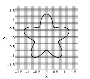
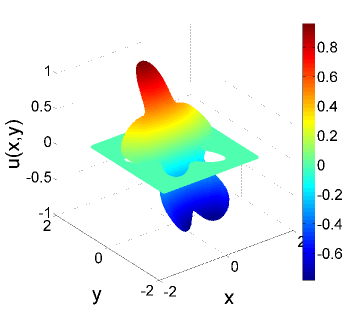
Figure 2: Left: solution domain $\Omega\/$ for example 1, embedded into a Cartesian grid. Right: solution obtained with the algorithm proposed in this paper.

Figure 3 illustrates the convergence of the method with a plot of the $L_{\infty}\/$ norm of the error versus $h\/$. The measured convergence rates are listed in table 1 at the end of this section. The measured rates indicate that the observed convergence is consistent with 4${}^{\textrm{th}}$ order in the Dirichlet case, and 3${}^{\textrm{rd}}$ order in the Neumann case. These results are as expected since we apply the algorithm with a combination of 4${}^{\textrm{th}}$ order numerical methods. The order loss in the Neumann problem occurs because the algorithm requires the computation of $v_{m}\/$ along $\partial\Omega\/$.

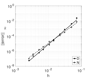
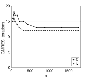
Figure 3: Left: error convergence for the Dirichlet and Neumann Poisson problems in example 1. Error is measured in the $L_{\infty}\/$ norm. The straight lines were obtained by least squares fits and their slopes correspond to the measured convergence rates – see table 1. Right: number of GMRES iterations needed to compute the potential distributions at the boundary $\partial\Omega\/$. Here $n$ indicates the number of markers used to discretize the boundary.

Figure 3 also shows the number of GMRES iterations needed to compute the potential distribution of the boundary integral formulation. No preconditioner is used, and the residual tolerance is set to $10^{-10}$. This figure shows that GMRES converges with a relatively small number of iterations, and that the number of iterations that does not depend on the size of the problem. These observations indicate that GMRES is an adequate solver for this problem.

5.2 Example 2. Open space problem with a discontinuity interface

In this example we solve the Poisson problem, defined in $\mathbb{R}^{2}\/$, associated with the exact solution

$$u^{+}(x,\,y) =\exp(-(x^{2}+y^{2})/0.0008)\/,$$ (52a)

$$\rule{0.0pt}{11.00008pt}u^{-}(x,\,y) =\cos\/(x)\sin\/(y)+1.5\/.$$ (52b)

The discontinuity interface, $\Gamma\/$, is defined by the curve (49), with parameters $\delta=0.03\/$ and $r_{0}=0.1\/$. Furthermore, we consider two cases in which the coefficients $\beta^{\pm}\/$ have large jumps across the discontinuity interface:

1. $\beta^{-}=1\/$, $\beta^{+}=10^{6}\/$,

2. $\beta^{-}=10^{6}\/$, $\beta^{+}=1$.

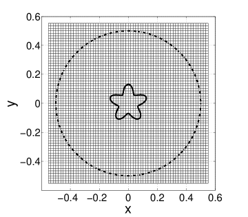
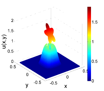
Figure 4: Left: computational box $\mathcal{B}\/$ used in example 2. The solid black line represents the interface $\Gamma\/$, and the dashed line is the circle that defines the support of the source term. Right: solution obtained with the algorithm proposed in this paper.

Note that the source term decays rapidly, such that we can consider $f^{+}(r)\approx 0\/$ for $r>0.4\/$. Hence, we set $\Omega_{f}=\{r|r\leq 0.4\}\/$ and solve the problem in a square region slightly larger than $\Omega_{f}\/$.

In addition, case (ii) is an example of the poorly conditioned problems discussed in §2.3. Thus, a direct application of any solution algorithm can lead to poor results in this case. For this reason we apply the prescription in §4.7 and impose the constraint:

$$\int_{\Gamma}\rho_{\Gamma}\,d\/S=-2.4846\/.$$ (53)

As shown in §4.7, this constraint can be computed with the original problem’s data. The right hand side in (53) is computed using Gaussian quadrature, and the constraint is implemented with the four digits of accuracy shown above. Figure 4 shows the solution to case (ii) computed with (53). This solution is visually indistinguishable from the solution obtained in case (i).

Figure 5 shows the convergence of the error in the $L_{\infty}\/$ norm in both cases (i) and (ii). In case (ii) we plot the error obtained for the constrained and unconstrained problems. The measured convergence rates are listed in table 1 at the end of this section. As expected, the measured rates are 3${}^{\textrm{rd}}$ order for both cases: (i) and the constrained problem in (ii). The solution to the unconstrained problem results in $\mathcal{O}(1)\/$ errors, even though the residual produced by GMRES is smaller than $10^{-10}\/$ in all cases. This example shows how sensitive to errors the unconstrained problem becomes when $\beta^{-}/\beta^{+}\gg 1\/$. In calculations with smaller beta-ratios the convergence of the unconstrained problem can be ascertained to be 3${}^{\textrm{rd}}$ order.

Finally, figure 6 shows the number of iterations the Krylov solver (either GMRES or CG) requires to converge to a residual tolerance of $10^{-10}$. The Krylov solver is used to compute the potential distribution of the boundary integral formulation. The unconstrained problem results in a non-symmetric linear system that is solved using GMRES. On the other hand, the constrained problem results in an overdetermined linear system, and the normal equation is solved using CG. Figure 6 shows that the Krylov solvers converge with a relatively small number of iterations, and that the number of iterations that does not depend on the size of the problem. Note that no pre-conditioners are used with GMRES and CG.

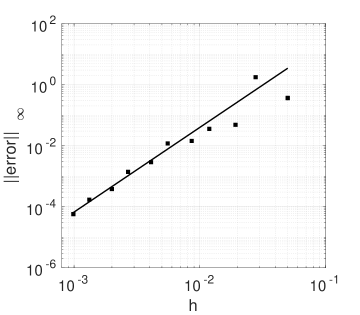
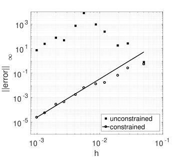
(a) case (i): $\beta^{-}=1\/$, $\beta^{+}=10^{6}\/$. (b) case (ii): $\beta^{-}=10^{6}\/$, $\beta^{+}=1\/$.

Figure 5: Error convergence: $L_{\infty}\/$ norm of the error for the Poisson problems with discontinuous coefficients in example 2. The straight lines were obtained by least squares fits and their slopes correspond to the measured convergence rates – see table 1.

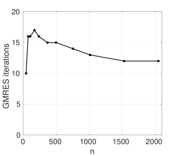
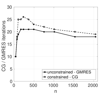
(a) case (i): $\beta^{-}=1\/$, $\beta^{+}=10^{6}\/$. (b) case (ii): $\beta^{-}=10^{6}\/$, $\beta^{+}=1\/$.

Figure 6: Convergence of Krylov solvers: number of iterations needed to compute the potential distributions at the interfaces $\Gamma\/$ and $\partial\Omega_{f}\/$. Here $n$ indicates the total number of markers used to discretize both interfaces.

5.3 Example 3. Interior Dirichlet and Neumann Poisson problems with a discontinuity interface

In this example, the solution domain is the unit disk, while the discontinuity interface is defined by (49) with parameters $\delta=0.1\/$ and $r_{0}=0.5\/$. Figure 7 shows the solution domain and the interface immersed in a regular Cartesian grid. In this domain, we solve the interior Dirichlet and Neumann Poisson problems associated with the exact solution

$$u^{+}(x,\,y) =x^{2}+y^{2}\/,$$ (54a)

$$\rule{0.0pt}{11.99998pt}u^{-}(x,\,y) =\cos\/(x)\,\sin\/(y)+2\/.$$ (54b)

Furthermore, as in §5.2, we consider two cases in which the coefficients $\beta^{\pm}\/$ have large jumps across the discontinuity interface:

1. $\beta^{-}=1\/$, $\beta^{+}=10^{6}\/$,

2. $\beta^{-}=10^{6}\/$, $\beta^{+}=1$.

Case (ii) is another instance of the poorly conditioned problem discussed in §2.3. Hence, in this example we apply the prescription in §4.7 and impose the constraint:

$$\rule{0.0pt}{16.99998pt}\int_{\Gamma}\rho_{\Gamma}\,d\/S=3.2044\/.$$ (55)

The right hand side in (55) is computed using Gaussian quadrature, and the constraint is implemented with the four digits of accuracy shown above.

In addition, the solutions to the Neumann problems are only defined up to an arbitrary constant. GMRES will automatically “pick” a constant, which may not correspond to (54). Hence, we shift the Neumann solutions to obtain $u^{-}(0,0)=2\/$. After this shift, the Dirichlet and Neumann solutions to case (i), and case (ii) with (55), become visually indistinguishable. Figure 7 shows the solution to the constrained Neumann problem in case (ii).

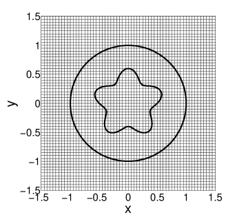
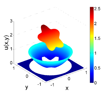
Figure 7: Left: solution domain $\Omega\/$ for example 3, embedded in a Cartesian Grid. The boundary $\partial\Omega\/$, and the discontinuity interface $\Gamma\/$, are the thick solid lines. Right: solution obtained with the algorithm proposed in this paper.

The convergence of error, measured in the $L_{\infty}\/$ norm, is displayed in figure 8. In case (ii) we plot the error obtained for the constrained and unconstrained problems. The measured convergence rates are listed in table 1 at the end of this section. As expected, we observe 3${}^{\textrm{rd}}$ order convergence for case (i) and the constrained problem of case (ii). Furthermore, the errors obtained for the unconstrained problem are significantly larger than the errors obtained for the constrained problem in case (ii).

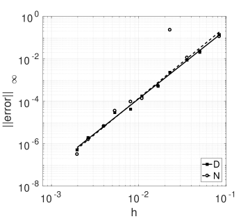
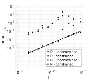
(a) case (i): $\beta^{-}=1\/$, $\beta^{+}=10^{6}\/$. (b) case (ii): $\beta^{-}=10^{6}\/$, $\beta^{+}=1\/$.

Figure 8: Error convergence: $L_{\infty}\/$ norm of the error for the Poisson problems with discontinuous coefficients in example 3. The straight lines were obtained by least squares fits and their slopes correspond to the measured convergence rates – see table 1.

Finally, figure 9 shows the number of iterations the Krylov solver (either GMRES or CG) requires to converge to a residual tolerance of $10^{-10}$. As in previous examples, no preconditioners were used. Once again we observe that the Krylov solvers converge with a relatively small number of iterations, and that the number of iterations that does not depend on the size of the problem.

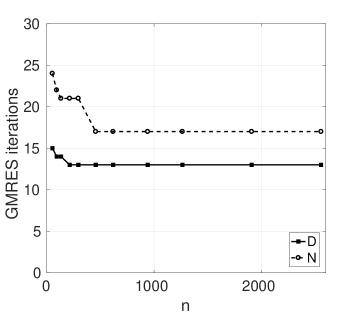
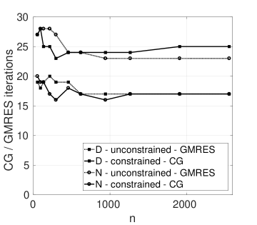
(a) case (i): $\beta^{-}=1\/$, $\beta^{+}=10^{6}\/$. (b) case (ii): $\beta^{-}=10^{6}\/$, $\beta^{+}=1\/$.

Figure 9: Convergence of Krylov solvers: number of iterations needed to compute the potential distributions at the interfaces $\Gamma\/$ and the boundary $\partial\Omega\/$. Here $n$ indicates the total number of markers used to discretize both the interface and the boundary.

Table 1: Measured convergence rate of the error in the $L_{\infty}$ norm for examples 1 through 3 — see figures 3, 5, and 8. Error limits correspond to one standard deviation of the least squares error. Only solutions with error smaller than 0.01 were considered, since the measured convergence rates serve as estimates of the asymptotic order of accuracy of the algorithm.

Problem	Measured	Theoretical
	convergence	convergence
	rate	rate
Ex. 1 – Dirichlet	$3.8\pm 0.1$	4.0
Ex. 1 – Neumann	$3.2\pm 0.1$	3.0
Ex. 2 – case (i)	$2.8\pm 0.2$	3.0
Ex. 2 – case (ii) constrained	$3.1\pm 0.1$	3.0
Ex. 3 – case (i) – Dirichlet	$3.3\pm 0.1$	3.0
Ex. 3 – case (i) – Neumann	$3.4\pm 0.3$	3.0
Ex. 3 – case (ii) constrained – Dirichlet	$3.3\pm 0.1$	3.0
Ex. 3 – case (ii) constrained – Neumann	$3.1\pm 0.1$	3.0

6 Conclusion

In this paper we presented an algorithm to solve Poisson problems in arbitrarily shaped domains immersed in regular Cartesian grids. The algorithm can be applied to a wide range of Poisson problems, including cases with prescribed internal jumps on both the solution and the weighted normal derivatives (with prescribed weights on each side). In particular, we showed that the algorithm produces good results even when the ratio between the weights is very large — as is the case in many multi-phase flow applications.

Mayo and collaborators [8, 12, 13] proposed a similar method for the Laplace and Poisson equations in an immersed setting. However, they considered only the case of immersed boundaries, and not interfaces of discontinuity. Furthermore, extensions of their method to general order of accuracy do not seem to be straightforward. In contrast, because we use the Correction Function Method (CFM), our method (at least in principle) can be readily extended to any desired order of accuracy.

The algorithm presented here relies on efficient and accurate numerical methods. The algorithm is comprised of three sub-problems: a boundary integral equation, and two “constant coefficients” Poisson problems defined in rectangular domains . The boundary integral equation is solved using well established boundary integral methods (BIM), whereas the Poisson equations are solved with finite differences and the CFM.

The accuracy of the algorithm was illustrated with several 2-D examples. The version of the algorithm implemented achieved 3${}^{\textrm{rd}}$ or 4${}^{\textrm{th}}$ order of accuracy, depending on the characteristics of the problem. However, the BIM and CFM may be implemented to any order of accuracy. Hence, there is no inherent limit to the accuracy that can be achieved with the algorithm proposed here.

Finally, the algorithm can be extended to 3-D. We have not yet implemented the algorithm in 3-D because the evaluation of the integrals in equation (30f) becomes an efficiency bottleneck. However, recent work [14] on the Kernel-Free Boundary Integral Method (KFBIM) provides a natural path for addressing this issue. Currently we are investigating the joint use of the CFM and the KFBIM for the purpose of obtaining an algorithm that is both high order (as the algorithm in this paper), and also efficient in 3-D.

References

- [1] A. N. Marques, J.-C. Nave, R. R. Rosales, A Correction Function Method for Poisson problems with interface jump conditions, Journal of Computational Physics 230 (20) (2011) 7567–7597. doi:10.1016/j.jcp.2011.06.014.
- [2] A. Mikhlin, A. Armstrong, Integral Equations and their Applications to Certain Problems Mechanics, Mathematical Physics and Technology, International Series of Monographs in the Science of the Solid State, Elsevier Science & Technology, 1957.
- [3] K. Atkinson, The numerical solution of integral equations of the second kind, Cambridge monographs on applied and computational mathematics, Cambridge University Press, 1997.
- [4] W. Mclean, Strongly elliptic systems and boundary integral equations, Cambridge University Press, 2000.
- [5] C. S. Peskin, Numerical analysis of blood flow in the heart, Journal of Computational Physics 25 (3) (1977) 220–252. doi:10.1016/0021-9991(77)90100-0.
- [6] R. J. LeVeque, Z. Li, The immersed interface method for elliptic equations with discontinuous coefficients and singular sources, SIAM Journal on Numerical Analysis 31 (4) (1994) 1019–1044. doi:10.1137/0731054.
- [7] R. P. Fedkiw, T. Aslam, S. Xu, The ghost fluid method for deflagration and detonation discontinuities, Journal of Computational Physics 154 (2) (1999) 393–427. doi:10.1006/jcph.1999.6320.
- [8] A. Mayo, The fast solution of Poisson’s and the biharmonic equations on irregular regions, SIAM Journal on Numerical Analysis 21 (2) (1984) 285–299. doi:10.1137/0721021.
- [9] V. Rokhlin, Rapid solution of integral equations of classical potential theory, Journal of Computational Physics 60 (2) (1985) 187–207. doi:10.1016/0021-9991(85)90002-6.
- [10] F. X. Canning, Sparse approximation for solving integral equations with oscillatory kernels, SIAM Journal on Scientific and Statistical Computing 13 (1) (1992) 71–87. doi:10.1137/0913004.
- [11] K. Nabors, F. T. Korsmeyer, F. T. Leighton, J. White, Preconditioned, adaptive, multipole-accelerated iterative methods for three-dimensional first-kind integral equations of potential theory, SIAM Journal on Scientific Computing 15 (3) (1994) 713–735. doi:10.1137/0915046.
- [12] A. Mayo, The rapid evaluation of volume integrals of potential theory on general regions, Journal of Computational Physics 100 (2) (1992) 236–245. doi:10.1016/0021-9991(92)90231-M.
- [13] A. McKenney, L. Greengard, A. Mayo, A fast poisson solver for complex geometries, Journal of Computational Physics 118 (2) (1995) 348 – 355. doi:10.1006/jcph.1995.1104.
- [14] W. Ying, W.-C. Wang, A kernel-free boundary integral method for implicitly defined surfaces, Journal of Computational Physics 252 (0) (2013) 606–624. doi:10.1016/j.jcp.2013.06.019.
- [15] H. Johansen, P. Colella, A Cartesian grid embedded boundary method for Poisson’s equation on irregular domains, Journal of Computational Physics 147 (1) (1998) 60–85. doi:10.1006/jcph.1998.5965.
- [16] A. M. Roma, C. S. Peskin, M. J. Berger, An adaptive version of the immersed boundary method, Journal of Computational Physics 153 (2) (1999) 509 – 534. doi:10.1006/jcph.1999.6293.
- [17] M.-C. Lai, C. S. Peskin, An immersed boundary method with formal second-order accuracy and reduced numerical viscosity, Journal of Computational Physics 160 (2) (2000) 705–719. doi:10.1006/jcph.2000.6483.
- [18] R. J. LeVeque, Z. Li, Immersed interface methods for Stokes flow with elastic boundaries or surface tension, SIAM Journal on Scientific Computing 18 (3) (1997) 709–735. doi:10.1137/S1064827595282532.
- [19] C. Zhang, R. J. LeVeque, The immersed interface method for acoustic wave equations with discontinuous coefficients, Wave Motion 25 (3) (1997) 237 – 263. doi:10.1016/S0165-2125(97)00046-2.
- [20] T. Y. Hou, Z. Li, S. Osher, H. Zhao, A hybrid method for moving interface problems with application to the Hele-Shaw flow, Journal of Computational Physics 134 (2) (1997) 236 – 252. doi:10.1006/jcph.1997.5689.
- [21] Z. Li, M.-C. Lai, The immersed interface method for the Navier-Stokes equations with singular forces, Journal of Computational Physics 171 (2) (2001) 822–842. doi:10.1006/jcph.2001.6813.
- [22] L. Lee, R. J. LeVeque, An immersed interface method for incompressible Navier-Stokes equations, SIAM Journal on Scientific Computing 25 (3) (2003) 832–856. doi:10.1137/S1064827502414060.
- [23] R. P. Fedkiw, T. Aslam, B. Merriman, S. Osher, A non-oscillatory Eulerian approach to interfaces in multimaterial flows (the ghost fluid method), Journal of Computational Physics 152 (2) (1999) 457–492. doi:10.1006/jcph.1999.6236.
- [24] X.-D. Liu, R. P. Fedkiw, M. Kang, A boundary condition capturing method for Poisson’s equation on irregular domains, Journal of Computational Physics 160 (1) (2000) 151–178. doi:10.1006/jcph.2000.6444.
- [25] M. Kang, R. P. Fedkiw, X.-D. Liu, A boundary condition capturing method for multiphase incompressible flow, Journal of Scientific Computing 15 (2000) 323–360. doi:10.1023/A:1011178417620.
- [26] D. Q. Nguyen, R. P. Fedkiw, M. Kang, A boundary condition capturing method for incompressible flame discontinuities, Journal of Computational Physics 172 (1) (2001) 71–98. doi:10.1006/jcph.2001.6812.
- [27] F. Gibou, L. Chen, D. Nguyen, S. Banerjee, A level set based sharp interface method for the multiphase incompressible Navier-Stokes equations with phase change, Journal of Computational Physics 222 (2) (2007) 536–555. doi:10.1016/j.jcp.2006.07.035.
- [28] D. B. Stein, R. D. Guy, B. Thomases, Immersed boundary smooth extension: A high–order method for solving PDE on arbitrary smooth domains using fourier spectral methods, Journal of Computational Physics 304 (2016) 252–274. doi:10.1016/j.jcp.2015.10.023.
- [29] A. Guittet, M. Lepilliez, S. Tanguy, F. Gibou, Solving elliptic problems with discontinuities on irregular domains: the Voronoi interface method, Journal of Computational Physics 298 (2015) 747 – 765. doi:10.1016/j.jcp.2015.06.026.
- [30] J. Dolbow, I. Harari, An efficient finite element method for embedded interface problems, International Journal for Numerical Methods in Engineering 78 (2) (2009) 229–252. doi:10.1002/nme.2486.
- [31] N. Moës, J. Dolbow, T. Belytschko, A finite element method for crack growth without remeshing, International Journal for Numerical Methods in Engineering 46 (1) (1999) 131–150. doi:10.1002/(SICI)1097-0207(19990910)46:1$<$131::AID-NME726$>$3.0.CO;2-J.
- [32] J. Bedrossian, J. H. von Brecht, S. Zhu, E. Sifakis, J. M. Teran, A second order virtual node method for elliptic problems with interfaces and irregular domains, Journal of Computational Physics 229 (18) (2010) 64050–6426. doi:10.1016/j.jcp.2010.05.002.
- [33] Z. Li, T. Lin, X. Wu, New cartesian grid methods for interface problems using the finite element formulation, Numerische Mathematik 96 (2003) 61–98. doi:10.1007/s00211-003-0473-x.
- [34] S. Hou, X.-D. Liu, A numerical method for solving variable coefficient elliptic equation with interfaces, Journal of Computational Physics 202 (2) (2005) 411–445. doi:10.1016/j.jcp.2004.07.016.
- [35] Z. Li, K. Ito, The immersed interface method: numerical solutions of PDEs involving interfaces and irregular domains, Frontiers in applied mathematics, SIAM, Society for Industrial and Applied Mathematics, 2006.
- [36] Y. Gong, B. Li, Z. Li, Immersed-interface finite-element methods for elliptic interface problems with nonhomogeneous jump conditions, SIAM Journal on Numerical Analysis 46 (1) (2008) 472–495. doi:10.1137/060666482.
- [37] J.-S. Huh, J. A. Sethian, Exact subgrid interface correction schemes for elliptic interface problems, Proceedings of the National Academy of Sciences 105 (29) (2008) 9874–9879. doi:10.1073/pnas.0707997105.
- [38] F. Gibou, R. Fedkiw, A fourth order accurate discretization for the Laplace and heat equations on arbitrary domains, with applications to the Stefan problem, Journal of Computational Physics 202 (2) (2005) 577–601. doi:10.1016/j.jcp.2004.07.018.
- [39] A. Mayo, High order accurate particular solutions to the biharmonic equation on general regions, Contemporary Mathematics 323 (2003) 233–243.
- [40] A. Mayo, A. Greenbaum, Fourth order accurate evaluation of integrals in potential theory on exterior 3D regions, Journal of Computational Physics 220 (2) (2007) 900 – 914. doi:10.1016/j.jcp.2006.05.042.
- [41] J. Romate, On the use of conjugate gradient-type methods for boundary integral equations, Computational Mechanics 12 (4) (1993) 214–232. doi:10.1007/BF00369963.
- [42] L. N. Trefethen, D. Bau, Numerical Linear Algebra, SIAM: Society for Industrial and Applied Mathematics, 1997.
- [43] L. C. Evans, Partial Differential Equations (Graduate Studies in Mathematics, V. 19) GSM/19, American Mathematical Society, 1998.
- [44] A. Mayo, A. Greenbaum, Fast parallel iterative solution of Poisson’s and the biharmonic equations on irregular regions, SIAM Journal on Scientific and Statistical Computing 13 (1) (1992) 101–118. doi:10.1137/0913006.
- [45] P. Brown, H. Walker, GMRES on (nearly) singular systems, SIAM Journal on Matrix Analysis and Applications 18 (1) (1997) 37–51. doi:10.1137/S0895479894262339.
- [46] W. Pogorzelski, Integral equations and their applications, International series of monographs in pure and applied mathematics, Pergamon Press, 1966.
- [47] J. Stoer, R. Bulirsch, Introduction to numerical analysis, Texts in applied mathematics, Springer, 2002.