Momentum transfer dependence of the proton’s electric and magnetic polarizabilities

Abstract

The $Q^{2}$-dependence of the sum of the electric and magnetic polarizabilities of the proton is calculated over the range $0\leq Q^{2}\leq 6$ GeV² using the generalized Baldin sum rule. Employing a parametrization of the $F_{1}$ structure function valid down to $Q^{2}=0.06$ GeV², the polarizabilities at the real photon point are found by extrapolating the results of finite $Q^{2}$ to $Q^{2}=0$ GeV². We determine the evolution over four-momentum transfer to be consistent with the Baldin sum rule using photoproduction data, obtaining $\alpha+\beta=13.7\pm 0.7\times 10^{-4}\,\text{fm}^{3}$.

I I.     Introduction

In order to study the internal structure of the nucleon, low-energy electron-proton scattering experiments are used to measure the response of the proton to an electromagnetic field. The electric ($\alpha$) and magnetic ($\beta$) polarizabilities are the fundamental parameters which describe this response. Physically, $\alpha$ and $\beta$ give a measure of the rigidity of the nucleon and are related to the unpolarized photoabsorption cross section by the Baldin sum rule Baldin (1960); Lapidus (1963),

$$\alpha+\beta=\frac{1}{4\pi^{2}}\int_{\nu_{\pi}}^{\infty}\frac{\sigma_{1/2}+\sigma_{3/2}}{\nu^{2}}\;d\nu,$$ (1)

where $\sigma_{\lambda}$ is cross section for the production of $\lambda=1/2,3/2$ helicity states, $\nu$ is the photon energy and $\nu_{\pi}$ the pion production threshold.

Further insight into the spatial distribution of the polarizabilities in the proton is gained from an understanding of the evolution of $\alpha$ and $\beta$ as a function of the four-momentum transfer, $Q^{2}$. Extending the above relation to incorporate this $Q^{2}$-dependence leads to the generalized Baldin sum rule Drechsel et al. (2003),

$$\alpha(Q^{2})+\beta(Q^{2}) = \frac{8\alpha_{\text{em}}M}{Q^{4}}\int_{0}^{x_{\pi}}\!xF_{1}(x,Q^{2})\,dx,$$

$$= 8\alpha_{\text{em}}M\int_{W_{\pi}^{2}}^{\infty}\frac{F_{1}(W^{2},Q^{2})}{\left(W^{2}-M^{2}+Q^{2}\right)^{3}}\,dW^{2}\!,$$

where $M$ is the mass of the proton, $\alpha_{\text{em}}$ is the fine structure constant, $x=Q^{2}/(W^{2}-M^{2}+Q^{2})$ is the Bjorken scaling variable and $W$ the invariant mass. $F_{1}$ is the proton’s electromagnetic structure function and we also note that in a similar manner to Eq. (1), $x_{\pi}$ and $W_{\pi}$ refer to the pion production point.

There has been considerable interest of late in accurately determining, both experimentally Liang et al. (2006) and theoretically Sibirtsev and Blunden (2013); Lensky and McGovern (2014), the $Q^{2}$-dependence of $\alpha$ and $\beta$. In Ref. Liang et al. (2006), Liang et al. exploited $e-p$ scattering data from the JLab E94-110 experiment Liang et al. (2004) to obtain $\alpha(Q^{2})+\beta(Q^{2})$ in the range $0.3<Q^{2}<4$ GeV². More recently, Sibirtsev and Blunden (SB) made use of updated data Liang et al. (2013) from the same experiment to construct a parametrization of the electromagnetic $F_{1}$ structure function Sibirtsev and Blunden (2013); Sibirtsev et al. (2010) which they then used to evaluate the Baldin integral. By doing so, they were able to provide valuable information on the low $Q^{2}$ properties of the electric and magnetic polarizabilities. Additionally, they found that the resonance region contribution dominates for $Q^{2}<1$ GeV² Sibirtsev and Blunden (2013).

In this report we improve upon the preceding work, utilizing the Adelaide-Jefferson Lab-Manitoba (AJM) parametrization of $F_{1}$ which is consistent down to much lower momentum transfer $\sim 0.06$ GeV². After a brief description of this construction in Sec. II, we evaluate the generalized Baldin sum rule, presenting our results in Sec. III. A discussion of their relation to those of Ref. Sibirtsev and Blunden (2013) is also included in this section, whilst final conclusions are given in Sec. IV.

II II.    Adelaide-Jefferson Lab-Manitoba parametrization

The parametrization of the $F_{1}$ structure function we employ in Eq. (LABEL:eqn:gBSR) was previously developed in Ref. Hall et al. (2013) for parity-violating asymmetry calculations. In this earlier work, the $Q^{2}$-$W^{2}$ plane of the structure function was separated into distinct regions according to the physics most appropriate to that region. At the low $Q^{2}$ and $W^{2}$, designated ‘Region I’, $F_{1}$ was given by Christy and Bosted’s (CB) fit Christy and Bosted (2010) to data from a 2008 version of Ref. Liang et al. (2004), with uncertainties of 3-5%. For the low $Q^{2}$ but high $W^{2}$ range (‘Region II’), a Regge parametrization was used in combination with the vector meson dominance model Sakurai and Schildknecht (1972); Alwall and Ingelman (2004). Finally, the high $Q^{2}$ and $W^{2}$ region was described by parton distribution functions given by Alekhin et al. Alekhin et al. (2012).

One additional constraint of the AJM parametrization was that at the boundary between the regions, the structure functions were required to match onto each other. Since the individual descriptions have areas in the $Q^{2}$-$W^{2}$ plane where they overlap, the position of the ‘hard’ borders should have little effect on the end result.

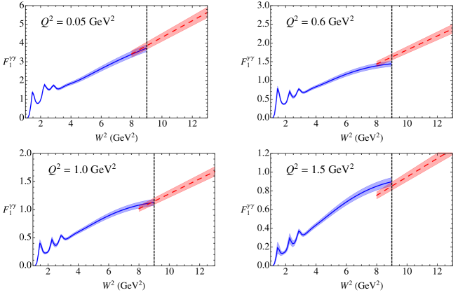
Figure 1: (color online) Proton $F_{1}$ structure function versus $W^{2}$ at fixed $Q^{2}=0.05$, 0.6, 1.0 and 1.5 GeV² for the CB fit Christy and Bosted (2010) at low $W^{2}$ (blue solid) and VMD+Regge parametrization Alwall and Ingelman (2004) at high $W^{2}$ (red dashed). The boundary between these is indicated by the vertical dashed line at $W^{2}=9$ GeV².

In Fig. 1 we plot $F_{1}(W^{2},Q^{2})$ as a function of $W^{2}$ for multiple values of $Q^{2}$ ranging from $Q^{2}=0.05$ to $1.5$ GeV². It is clear from these plots that the two descriptions of the structure function are in good agreement at the boundaries. The errors, shown by the shaded bands, come from assigning a conservative 5% uncertainty to both parametrizations of the structure function.

III III.    $Q^{2}$ dependence of $\alpha$ and $\beta$

As we would like to determine the evolution of the polarizabilities all the way to the photoproduction point, the behavior of the parametrization of $F_{1}$ at very low $Q^{2}$ is of particular importance. CB’s fit includes data to $Q^{2}$ as low as $0.06$ GeV² as well as photoproduction data, showing good agreement with the experimental values in the regions where there is data. However, as $Q^{2}\rightarrow 0$ the parametrization fails to accurately match onto the real photon point as a result of difficulties in correctly fitting the second resonance peak. In order to get around this problem, we determine $\alpha(Q^{2})+\beta(Q^{2})$ down to $Q^{2}=0.06$ GeV² using CB’s $F_{1}$, before extrapolating the results the rest of the way to $Q^{2}=0$ GeV². By fitting the results over several ranges of momentum transfer, we qualify any systematic uncertainty in this extrapolation.

In Fig. 2 we evaluate the generalized Baldin sum rule over the range $0.06\leq Q^{2}\leq 6$ GeV², also including the results of Ref. Sibirtsev and Blunden (2013). Although we show the $Q^{2}$-dependence up to $6$ GeV², the determination of the polarizabilities is limited only by the accuracy and validity of the PDFs. In principal, one could calculate the sum all the way up to LHC energies.

For the low-$Q^{2}$ behavior, as mentioned before, we fit the results for the Baldin integral (in this case using the inverse of a polynomial) over four different ranges of $Q^{2}$: (I) $0.04<Q^{2}<0.10$ GeV²; (II) $0.04<Q^{2}<0.12$ GeV²; (III) $0.06<Q^{2}<0.10$ GeV²; (IV) $0.06<Q^{2}<0.12$ GeV². These fits were then extrapolated to $Q^{2}=0$ GeV², with the results of the extrapolations in Fig. 3 showing minimal variation of $\alpha+\beta$ over the $Q^{2}$ ranges.

At the real photon point we obtain,

$$\alpha+\beta=(13.7\pm 0.7)\times 10^{-4}\;\text{fm}^{3}$$ (3)

where we quote results for the fit over the region (III). The error $\pm 0.7$ comes from the conservative 5% uncertainty associated with the CB parametrization. Our result is in excellent agreement with the previous determination of Babusci et al. Babusci et al. (1998), who quote

$$\alpha+\beta=(13.69\pm 0.14)\times 10^{-4}\;\text{fm}^{3}$$ (4)

and the more recent value,

$$\alpha+\beta=(13.8\pm 0.4)\times 10^{-4}\;\text{fm}^{3},$$ (5)

of Ref. Olmos de Leon et al. (2001).

As can be seen, our evaluation differs substantially from that of Ref. Sibirtsev and Blunden (2013). Most notably, as $Q^{2}$ tends to $0$ the sum of $\alpha(Q^{2})$ and $\beta(Q^{2})$ clearly converges to the value at the real photon point, whereas an extrapolation of the SB curve would overshoot this value significantly. The variation between the two results may be explained by the fact that the AJM parametrization uses the fit of CB for $F_{1}$ which is consistent to much lower $Q^{2}$ values. Although not shown on the graph and in agreement with SB, we found that the resonance contribution dominates at low $Q^{2}$. (We also point out that varying the $W^{2}$ boundary between Region I and II has a negligible effect on the final values.)

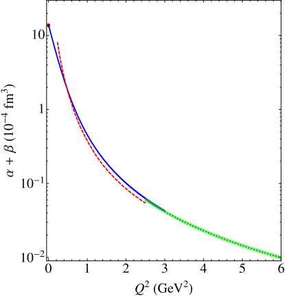
Figure 2: (color online) The sum of the electric and magnetic polarizabilities as a function of $Q^{2}$. The blue line (with errors) represents our calculation for $Q^{2}\leq 2.5$ GeV², the green dotted line for $Q^{2}>2.5$ GeV², whilst the red-dashed line is the earlier calculation of Ref. Sibirtsev and Blunden (2013). On this scale the values of $\alpha+\beta$ at the real photon point overlay each other and are given by the black triangle Babusci et al. (1998) and red square Olmos de Leon et al. (2001).

Additionally, we calculate the “radius” of the sum of the polarizabilities, i.e.,

$$\langle r^{2}\rangle=\left.\frac{-6}{H(0)}\frac{dH(Q^{2})}{dQ^{2}}\right|_{Q^{2}=0}$$ (6)

where in this case, $H(Q^{2})=\alpha(Q^{2})+\beta(Q^{2})$. For the fit used to determine the small-$Q^{2}$ extrapolation the radius is

$$\langle r^{2}\rangle_{\alpha+\beta}^{1/2}=0.98\pm 0.05\,\text{fm}.$$ (7)

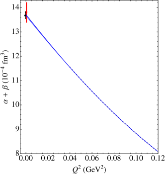
Figure 3: (color online) In this plot, the individual points are values extracted using the AJM parametrization, whilst the blue lines are fits to points over four distinct ranges in $Q^{2}$. The values of $\alpha+\beta$ at $Q^{2}=0$ GeV² have been offset slightly and are given by the black triangle Babusci et al. (1998) and red square Olmos de Leon et al. (2001).

IV IV.    Conclusion

Utilizing a description of the $F_{1}$ structure function which is consistent down to $0.06$ GeV² and extrapolating to $Q^{2}=0$ GeV², we have shown that the $Q^{2}$-dependence of the electric and magnetic polarizabilities matches accurately onto the dispersion relation at the real photon point. We explain the difference from the results of SB at low $Q^{2}$ from this property of our structure function. At higher $Q^{2}$, the difference arises primarily from the deviation of their model from the CB parametrization. Increased data at very low $Q^{2}$ and low $W^{2}$ region would be useful in decreasing the uncertainties still further.

References

- Baldin (1960) A. M. Baldin, Nuclear Physics 18, 310 (1960), ISSN 0029-5582.
- Lapidus (1963) L. I. Lapidus, Sov. Phys. JETP 16, 964 (1963).
- Drechsel et al. (2003) D. Drechsel, B. Pasquini, and M. Vanderhaeghen, Phys. Rept. 378, 99 (2003), eprint hep-ph/0212124.
- Liang et al. (2006) Y. Liang, M. E. Christy, R. Ent, and C. E. Keppel, Phys. Rev. C 73, 065201 (2006), eprint nucl-ex/0410028.
- Sibirtsev and Blunden (2013) A. Sibirtsev and P. G. Blunden (2013), eprint 1311.6482.
- Lensky and McGovern (2014) V. Lensky and J. A. McGovern (2014), eprint 1401.3320.
- Liang et al. (2004) Y. Liang et al. (2004), eprint nucl-ex/0410027v1.
- Liang et al. (2013) Y. Liang et al. (2013), eprint nucl-ex/0410027v2.
- Sibirtsev et al. (2010) A. Sibirtsev, P. G. Blunden, W. Melnitchouk, and A. W. Thomas, Phys. Rev. D 82, 013011 (2010), eprint 1002.0740.
- Hall et al. (2013) N. L. Hall, P. G. Blunden, W. Melnitchouk, A. W. Thomas, and R. D. Young, Phys. Rev. D 88, 013011 (2013), eprint 1304.7877.
- Christy and Bosted (2010) M. E. Christy and P. E. Bosted, Phys. Rev. C 81, 055213 (2010), eprint 0712.3731.
- Sakurai and Schildknecht (1972) J. J. Sakurai and D. Schildknecht, Phys. Lett. B 40, 121 (1972).
- Alwall and Ingelman (2004) J. Alwall and G. Ingelman, Phys. Lett. B 596, 77 (2004), eprint hep-ph/0402248.
- Alekhin et al. (2012) S. Alekhin, J. Blumlein, and S. Moch, Phys. Rev. D 86, 054009 (2012), eprint 1202.2281.
- Babusci et al. (1998) D. Babusci, G. Giordano, and G. Matone, Phys. Rev. C 57, 291 (1998), eprint nucl-th/9710017.
- Olmos de Leon et al. (2001) V. Olmos de Leon, F. Wissmann, P. Achenbach, J. Ahrens, H. Arends, et al., Eur. Phys. J. A10, 207 (2001).