On the active manipulation of EM fields in open waveguides

Abstract

In this paper we present the extension of the results proposed in [53] and study the problem of active control of TM waves propagating in a waveguide. The main goal is to cancel, in a prescribed near field region, the longitudinal component of the electric field of an incoming TM wave while having vanishingly small fields near the waveguide boundary. The main analytical challenge is to design appropriate source functions for the scalar Helmholtz equation so that the desired cancellation effect will be obtained. We show the existence of a class of solutions to the problem and provide numerical support of the results. Discussion on the feasibility of the proposed approach as well as possible design strategies are offered.

Key words. Field manipulation, Helmholtz equation, waveguides, layer potentials, integral equation, antenna synthesis, active exterior cloaking.

1 Introduction

The technique of manipulating acoustic and electromagnetic fields in desired regions of space has advanced in the recent years, with fascinating applications, such as cloaking, the creation of illusions, secure remote communication, focusing energy, and novel imaging techniques. The development can be roughly classified into two categories.

One main approach controls fields in the regions of interest by changing the material properties of the medium in certain surrounding regions while a second approach actively manipulates (active control) specially designed sources (antennas). Thus, briefly, we distinguish passive from active methods by the use of sources in the latter approach.

In [9] (see also [11]) the authors presented an early rigorous discussion of the passive manipulation of fields in the context of quasistatics cloaking (see also [32], [33] and [34] where the invariance to a change of variables is fully explained and the transformed material are described). This work was later extended in [26] to the general case of passive manipulation of fields in the finite frequency regime (see also the review [4] and references therein). These passive strategies are now known as “transformation optics”. The similar strategy in the context of acoustics was proposed in [10] (see also [7] and the review [3] and references therein). The idea behind transformation optics/acoustics is the invariance of the corresponding Dirichlet to Neumann-map (boundary measurements map) considered on some external boundary with respect to suitable change of variables which are identity on the respective boundary. This invariance result implies that two different materials (the initial one and the one obtained after the change of variables is applied) occupying some region of space $\Omega$, will have the same boundary measurements maps on $\partial\Omega$ and thus be equivalent from the point of view of an external observer. This mathematical structure leads to important applications, such as cloaking, field concentrators ([39]) or field rotators, illusion optics, etc. (see [4], [3], [8], [1] and references therein), and sensor cloaking while maintaining sensing capability [48], [49].

Additional passive techniques proposed in the literature (other than transformation optics strategies) include, plasmonic designs (see [1] and references therein), strategies based on anomalous resonance phenomena (see [23], [25], [24]), conformal mapping techniques (see [21],[20]), and complimentary media strategies (see [19]).

Active designs for the manipulation of fields appear to have occurred initially in the context of low-frequency acoustics (or active noise cancellation). Especially notable are pioneer works of Leug [46] (feed-forward control of sound) and Olson & May [47] (feedback control of sound). The reviews [42], [44], [45], [40] [41] provide detailed accounts of past and recent developments in acoustic active control.

Active control strategies are based on Huygens principle. The interior active cloaking strategy proposed in [22] employs active boundaries while the exterior active cloaking scheme discussed in [13], [14], [15], [12] (see also [50]) uses a discrete number of active sources (antennas) to manipulate the fields. The active exterior strategy for 2D quasistatics cloaking was introduced in [13], and based on a priori information about the incoming field. Guevara Vasquez, Milton and Onofrei [13] constructively described how one can create an almost zero field external region while maintaining a very small scattering effect in the far field. The proposed strategy did not work for objects close to the antennas, it cloaked large objects only when they are far enough to the antenna (see [12]). Also, the method was not adaptable for three space dimensions. The finite frequency case was studied in the last section of [13] and in [15] (see also [12] for a recent review) where three active sources (antennas) were needed to create a zero field region in the interior of their convex hull while creating a very small scattering effect in the far field. The broadband character of the proposed scheme was numerically observed in [14]. A general approach, based on the theory of boundary layer potentials, is proposed in [53] for the solution of the active manipulation of quasi-static fields with one active source (antenna). Several authors proposed experimental designs of active cloaking schemes in various regimes, [57], [58], [56] and [59]. In this paper, we extend the results presented in [53] to the case of locally nulling TM modes propagating in an open circular waveguide. The mathematical problem is formulated in the context of the scalar Helmholtz equation and the feasibility study discusses the relevance of this analysis in the context of a real antenna placed inside the waveguide and carrying electric conduction currents.

The paper is organized as follows: In Section 2 we introduce the main problem of local nulling a waveguide TM mode (Question 1). Then, in Section 3 we prove the mathematical existence of a class of solutions for Question 1 and in 4 we offer several numerical simulations to support our results. Antenna feasibility considerations and possible design strategies are discussed in Section  5.

2 Problem formulation

In this paper $B_{r}({\bf x})$ will denote the disk situated in a plane perpendicular on the $Ox$ axis centered in point ${\bf x}\in{\mathbb{R}}^{3}$ and of radius $r>0$. Consider the waveguide $D$, given by $D=(-\infty,+\infty)\times B_{R}({\bf 0})$, i.e, a circular cylinder of cross sectional area $B_{R}({\bf 0})$ and of infinite extent in the $Ox$ direction. We further consider that $D$ is a hollow waveguide filled with air and that the walls of the waveguide are made of perfect conductors. In reality the waveguide walls have some level of loss, and by using the results of [60], we see that the assumption of zero loss provides a very good approximation for the case of small losses. Inside the cylinder we consider an antenna (fixed there by a transparent dielectric), occupying the region $D_{a}$ which is modeled as a coaxial cylinder with smooth enough boundary and small cross sectional area, (Figure 1 describes a the geometry for an antenna with straight edges).

The region of interest (control region) will be denoted by $D_{c}$, and it will be assumed to be an open domain with $D_{c}\subsetneq D\setminus{\bar{D}}_{a}$. In Section 4 we will assume $D_{c}$ to be an annular shell coaxial with and in the near field of the antenna $D_{a}$, defined by $D_{c}=\{B_{\delta+l_{1}+l_{2}}({\bf 0})\setminus B_{\delta+l_{1}}({\bf 0})\}\times[-a,a]$, where $l_{1},l_{2},a$ are given positive reals (see also Figure 1). Let us next denote by $({\bf E}_{i},{\bf B}_{i})$ a given incoming field propagating down the waveguide and by $E_{xi}$ the longitudinal component of its electric field. The general question we want to study is:

Question 1.

Can we synthesize an active source (antenna) $D_{a}$ (to be placed inside the waveguide $D$ as in Figure 1), modeled as a magnetic current ${\bf M}({\bf x})$ supported on $\partial D_{a}$, such that the field generated by it, $({\bf E}_{s},{\bf B}_{s})$, with ${\bf E}_{s}=(E_{xs},E_{ys},E_{zs})$ and ${\bf B}_{s}=(B_{xs},B_{ys},B_{zs})$, has the property that in the region of interest $D_{c}$, $E_{xs}$ almost cancels $E_{xi}$? (Note that in the sketch of Figure 1 we only presented a cylindrical antenna with straight edges although in practice one will consider the antenna with a smooth surface, e.g., cylindrical shape with hemispherical edges).

We divide the general problem presented in Question 1 in two subproblems:

• Problem 1. Show that there exists boundary data $E_{b}$, such that $u$, the solution of the exterior Dirichlet problem for the Helmholtz equation with $E_{b}$ specified on $\partial D_{a}$, has the property that in the region of interest $D_{c}$ it almost cancels $E_{xi}$ while having vanishingly small values on the boundary of the waveguide?

• Problem 2. Based on the result of Problem 1, can we synthesize an active source (antenna) $D_{a}$ (to be placed inside the waveguide $D$ as in Figure 1), modeled as a surface magnetic current ${\bf M}({\bf x})$ supported on $\partial D_{a}$ such that $E_{xs}$, the longitudinal component of its electric field, will be very close to $u$ described above and thus will posses the desired control properties?

We mention that Problem 1 above studies the existence of solutions for a class of exterior Helmholtz problems which, as will be proved in Section 5, are essential in showing the existence of solutions for Question 1. On the other hand, Problem 2 above studies the feasibility of the antenna synthesis question. In this paper we will focus on Problem 1 above in Section 3 and Section 4 and present a brief feasibility study in Section 5. A much more detailed discussion about the feasibility of the second step in the context of the general antenna synthesis problem will be soon presented in [55].

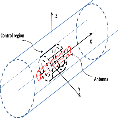
Figure 1: The geometrical setting of Formulation A.

3 Existence results

A schematic illustration of the problem setting (where we assumed for simplification straight antenna edges) and various geometrical parameters are shown in Figure  1. Assume a general TM incoming electromagnetic wave $({\bf B}_{i},{\bf E}_{i})$ with ${\bf B}_{i}=(0,B_{yi},B_{zi})$ and ${\bf E}_{i}=(E_{xi},E_{yi},E_{zi})$. By recalling that each component of the electric and magnetic field satisfy the 3D scalar Helmholtz equation in their domain of analyticity, by using the boundary conditions on the surface of the waveguide, Problem 1 of Question 1 reduces to the following mathematical formulation,

Mathematical equivalent of Problem 1

Let $0<\varepsilon\ll 1$ be fixed and assume $-\lambda^{2}$ is not a Neumann eigenvalue for the Laplacean in $D_{a}$. Consider an incoming TM wave $({\bf E}_{i},{\bf B}_{i})$ and let $E_{xi}$ be the longitudinal component of its electric field. Then the equivalent mathematical formulation for Problem 1 of Question 1 reads:

Problem 1*. Find $E_{b}\in C(\partial D_{a})$ such that there exists $u\in H^{1}({\mathbb{R}}^{3}\setminus{\bar{D}}_{a})$ satisfying,

$$\vspace{0.15cm}\left\{\vspace{0.15cm}\begin{array}[]{llll}\Delta u+\lambda^{2}u=0\mbox{ in }{\mathbb{R}}^{3}\setminus\overline{D}_{a}\vspace{0.15cm}\\ u=E_{b}\mbox{ on }\partial D_{a}\vspace{0.15cm}\\ \displaystyle\left(\frac{x}{|x|},\nabla u(x))-iku(x)\right)=o\left(\frac{1}{|x|}\right),\mbox{ as }|x|\rightarrow\infty,\mbox{ uniformly for all directions $\displaystyle\frac{x}{|x|}$ }\end{array}\right.,$$

and

$$\|u\|_{L^{2}(\partial D)}\leq\varepsilon,\;\|u+E_{xi}\|_{H^{1}({\bar{D}_{c}})}\leq\varepsilon.$$ (3.1)

It is well known that, (see [6]), given $E_{b}\in C(\partial D_{a})$, Problem 1*. has a unique solution in $H^{1}({\mathbb{R}}^{3}\setminus{\bar{D}}_{a})$ for all $\lambda$ satisfying the above assumptions.

Thus, it remains to be proved that one can find a boundary data $E_{b}\in C(\partial D_{a})$ so that the estimates (3.1) are satisfied. For $L>0$ large enough consider $D_{L}$ sooth sub-domain of ${\mathbb{R}}^{3}$ defined by

$$\{(x,y,z)\in D,|x|<L\}\subset D_{L}\subset\{(x,y,z)\in D,|x|<2L\}$$ (3.2)

In what follows we make the assumption that the antenna, the region of control and the boundary of the waveguide are sufficiently well separated, i.e., there exist $D_{a^{\prime}},D_{1}$ smooth sub-domains of ${\mathbb{R}}^{3}$ so that

$$D_{c}\subsetneq D_{1}\subsetneq D_{L}\setminus{\bar{D}}_{a}.$$ (3.3)

Consider also

$$D_{a^{\prime}}\subsetneq D_{a}$$ (3.4)

In what follows we will also make the following assumption:

$$-\lambda^{2}\mbox{ is not a Laplace Dirichlet eigenvalue in $D_{1}$. }$$ (3.5)

Note that the set $D_{1}$ in (3.3) can be chosen so that (3.5) is as well satisfied. We next introduce the following space $\Xi$,

$$\Xi\equiv L^{2}(\partial D_{1})\times L^{2}(\partial D_{L}).$$ (3.6)

Then $\Xi$ is a Hilbert space with respect to the scalar product given by

$$(\varphi,\psi)_{\Xi}=\int_{\partial D_{1}}\varphi_{1}({\bf y}){\overline{\psi}}_{1}({\bf y})ds_{{\bf y}}+\int_{\partial D_{L}}\varphi_{2}({\bf y}){\overline{\psi}}_{2}({\bf y})ds_{{\bf y}},$$ (3.7)

for all $\varphi\equiv(\varphi_{1},\varphi_{2})$ and $\psi=(\psi_{1},\psi_{2})$ in $\Xi$ where $(\cdot)$ above, denotes the complex conjugate.

The next Theorem is the main result of the Section and it shows the existence of a sequence of solutions for problem (3), (3.1) such that Problem 1 of Question 1 will have a positive answer. We have:

Theorem 3.1.

Let $\lambda$ satisfying the hypothesis of ${\bf{Problem1*}}$ and (3.5). Consider the following integral operator, $K:L^{2}(\partial D_{a^{\prime}})\rightarrow\Xi$, defined as

$$Ku({\bf x},{\bf z})=(K_{1}u({\bf x}),K_{2}u({\bf z})),$$ (3.8)

for any $u({\bf x})\in L^{2}(\partial D_{a^{\prime}})$, where

$$K_{1}u({\bf x}) = \int_{\partial D_{a^{\prime}}}u({\bf y})\frac{\partial\Phi({\bf x},{\bf y})}{\partial\mbox{\boldmath${\nu}$}_{{\bf y}}}ds_{{\bf y}},\mbox{ for }{\bf x}\in\partial D_{1},$$

$$K_{2}u({\bf z}) = \int_{\partial D_{a^{\prime}}}u({\bf y})\frac{\partial\Phi({\bf z},{\bf y})}{\partial\mbox{\boldmath${\nu}$}_{{\bf y}}}ds_{{\bf y}},\mbox{ for }{\bf z}\in\partial D_{L},$$ (3.9)

with $\displaystyle\mbox{\boldmath${\nu}$}_{{\bf y}}$ denoting the normal exterior to $\partial D_{a^{\prime}}$ and where $\Phi({\bf x},{\bf y})$ represents the fundamental solution of the relevant Helmholtz operator, i.e.,

$$\Phi({\bf x},{\bf y})=\frac{e^{i\lambda|{\bf x}-{\bf y}|}}{|{\bf x}-{\bf y}|}.$$ (3.10)

Then, the operator $K$ is compact and has a dense range. Moreover, for $\alpha_{n}\rightarrow 0$ (i.e., Tikhonov regularizers) the functions $v_{n}\in C(\partial D_{a})$ defined by

$$v_{n}=(\alpha_{n}I+K^{*}K)^{-1}K^{*}v,\mbox{ with }v=(-E_{ix},0),$$ (3.11)

satisfy that, for any $\epsilon<<1$, there exists an $N_{\epsilon}\in\mathbb{N}$ such that for any $n>N_{\epsilon}$ the functions $u_{n}$ given by,

$$u_{n}=\int_{\partial D_{a^{\prime}}}v_{n}({\bf y})\frac{\partial\Phi({\bf x},{\bf y})}{\partial\nu_{\bf y}}ds_{\bf y}$$ (3.12)

satisfy,

$$\left\{\begin{array}[]{lll}\vspace{0.2cm}\Delta u_{n}+\lambda^{2}u_{n}=0,\mbox{ in }D\setminus{\bar{D}}_{a^{\prime}}&\vspace{0.2cm}\\ \|u_{n}\|_{L^{2}(\partial D)}\leq\varepsilon&\vspace{0.2cm}\\ \|u_{n}+E_{xi}\|_{H^{1}(D_{c})}\leq\varepsilon.\vspace{0.2cm}\end{array}\right.$$ (3.13)

Proof.

The next lemma presents a technical regularity results and it is needed in the proof of the Theorem.. Since the proof is classical we do not include it here but point out that the result can be obtained by adapting the proof in [18], (Section 3.4).

Lemma 3.1.

Let $\lambda\in{\mathbb{R}}$ as in Theorem 3.1. Let $f_{i}\in C(\partial D_{1}))$, and consider $v_{i}\in C^{2}(D_{1})\cap C(\overline{D_{1}})$ be the solution of the following interior Dirichlet problem,

$$\left\{\begin{array}[]{ll}\Delta v_{i}+\lambda^{2}v_{i}=0\mbox{ in }D_{1}\vspace{0.15cm}\\ v_{i}=f_{i}\mbox{ on }\partial D_{1}.\vspace{0.15cm}\end{array}\right.$$ (3.14)

Then we have,

$$\|v_{i}\|_{H^{1}(D_{c})}\leq C_{i}\|f_{i}\|_{L^{2}(\partial D_{1})},$$

where $C_{i}=C(\lambda,D_{c},D_{1})$.

We are now ready to present the proof of Theorem (3.1). Let us consider the integral operator, $K:L^{2}(\partial D_{a})\rightarrow\Xi$, defined at (3.9).

The next Lemma given without proof, is a simple consequence of classical results in potential theory.

Lemma 3.2.

The operator $K$ defined in (3.8) is a compact linear operator from $L^{2}(\partial D_{a^{\prime}})$ to $\Xi$.

Let us introduce further the adjoint operator of $K$, i.e., the operator $K^{*}:\Xi\rightarrow L^{2}(\partial D_{a^{\prime}})$ defined through the relation,

$$(Kv,u)_{\Xi}=(v,K^{*}u)_{L^{2}(\partial D_{a^{\prime}})},\ \forall u\in\Xi,v\in L^{2}(\partial D_{a^{\prime}}),$$ (3.15)

where $(\cdot,\cdot)_{\Xi}$ is the scalar product on $\Xi$ defined in (3.7) and $(\cdot,\cdot)_{L^{2}(\partial D_{a^{\prime}})}$ denotes the usual scalar product in $L^{2}(\partial D_{a^{\prime}})$ defined as a vectorial space over the complex field. We check, by simple change of variables and algebraic manipulations, that the adjoint operator $K^{*}$ is given by,

$$K^{*}u({\bf x})=\int_{\partial D_{1}}u_{1}({\bf y})\frac{\partial{\overline{\Phi}}({\bf x},{\bf y})}{\partial\mbox{\boldmath${\nu}$}_{{\bf x}}}ds_{{\bf y}}+\int_{\partial D_{L}}u_{2}({\bf y})\frac{\partial{\overline{\Phi}}({\bf x},{\bf y})}{\partial\mbox{\boldmath${\nu}$}_{{\bf x}}}ds_{{\bf y}},$$ (3.16)

for any $u=(u_{1},u_{2})\in\Xi$ and ${\bf x}\in\partial D_{a^{\prime}}$.

From the compactness and linearity of $K$ as given in Lemma 5.2, we conclude that the adjoint operator $K^{*}$ is compact as well. Furthermore, let us denote by ${\rm Ker}(K^{*})$ the kernel (i.e., null space) of $K^{*}$. Then we have the following result.

Proposition 3.1.

If $\psi=(\psi_{1},\psi_{2})\in{\rm Ker}(K^{*})$ then $\psi\equiv(0,0)$ in $\Xi$.

Proof.

Let $\psi\in{\rm Ker}(K^{*})$ and define

$$w({\bf x})=\int_{\partial D_{1}}{\overline{\psi}}_{1}({\bf y})\Phi({\bf x},{\bf y})ds_{{\bf y}}+\int_{\partial D_{L}}{\overline{\psi}}_{2}({\bf y})\Phi({\bf x},{\bf y})ds_{{\bf y}}\mbox{ for }{\bf x}\in{\mathbb{R}}^{3},$$ (3.17)

where the integrals exist as improper integrals for ${\bf x}\in\partial D_{1}\cup\partial D_{L}$. From $K^{*}\psi=0$ and (3.16) we have that $w$ satisfies the Laplace equation

$$\left\{\vspace{0.15cm}\begin{array}[]{ll}\Delta w+\lambda^{2}w=0,&\mbox{ in }D_{a^{\prime}}\vspace{0.15cm}\\ \displaystyle\frac{\partial w}{\partial\mbox{\boldmath${\nu}$}_{{\bf x}}}=0,&\mbox{ on }\partial D_{a^{\prime}}.\end{array}\right..$$ (3.18)

We then conclude that

$$w=0\mbox{ in }D_{a^{\prime}}.$$ (3.19)

Then, because by definition $w$ is a solution of Helmholtz equation in $D_{L}\setminus{\bar{D}}_{1}$, by analytic continuation we conclude that

$$w=0\mbox{ in }D_{L}\setminus{\bar{D}}_{1}.$$ (3.20)

The next relations for $w$ are in fact the classical jump conditions for the single layer potentials with $L^{2}$ densities (see [5] and references therein). We have,

$$\displaystyle\lim_{h\rightarrow 0^{+}}\int_{\partial D_{1}}|w({\bf x}\pm h\mbox{\boldmath${\nu}$}_{{\bf x}})-w({\bf x})|^{2}ds_{{\bf x}}=0$$ (3.21)

$$\displaystyle\lim_{h\rightarrow 0^{+}}\int_{\partial D_{L}}|w({\bf x}\pm h\mbox{\boldmath${\nu}$}_{{\bf x}})-w({\bf x})|^{2}ds_{{\bf x}}=0$$ (3.22)

$$\displaystyle\lim_{h\rightarrow 0^{+}}\int_{\partial D_{1}}\left|2\frac{\partial w}{\partial\mbox{\boldmath${\nu}$}_{{\bf x}}}({\bf x}\pm h\mbox{\boldmath${\nu}$}_{{\bf x}})-2\frac{\partial w}{\partial\mbox{\boldmath${\nu}$}_{{\bf x}}}({\bf x})\pm\psi_{1}({\bf x})\right|^{2}ds_{{\bf x}}=0$$ (3.23)

$$\displaystyle\lim_{h\rightarrow 0^{+}}\int_{\partial D_{L}}\left|2\frac{\partial w}{\partial\mbox{\boldmath${\nu}$}_{{\bf x}}}({\bf x}\pm h\mbox{\boldmath${\nu}$}_{{\bf x}})-2\frac{\partial w}{\partial\mbox{\boldmath${\nu}$}_{{\bf x}}}({\bf x})\pm\psi_{2}({\bf x})\right|^{2}ds_{{\bf x}}=0,$$ (3.24)

where $\mbox{\boldmath${\nu}$}_{\bf x}=\mbox{\boldmath${\nu}$}({\bf x})$ denotes the exterior normal to $\partial D_{L}$ and $\partial D_{1}$ respectively and all the integral of the normal derivatives of $w$ exists as improper integrals. From (3.20), (3.21) and (3.22) we obtain that

$$w=0\mbox{ on }\partial D_{L}\cup\partial D_{1}.$$ (3.25)

Next from (3.5) and by uniqueness of the interior Dirichlet problem for $w$ on $D_{1}$ and (3.25) we obtain

$$w=0\mbox{ in }\bar{D}_{1}.$$ (3.26)

From (3.20), (3.26), and the two jump relations (3.23), we obtain that

$$\psi_{1}=0\mbox{ on }\partial D_{1}.$$ (3.27)

Equation (3.27) used in the definition of $w$ given at (3.17), implies

$$w({\bf x})=\int_{\partial D_{L}}{\overline{\psi}}_{2}({\bf y})\Phi({\bf x},{\bf y})ds_{{\bf y}},\mbox{ for }{\bf x}\in{\mathbb{R}}^{3}.$$ (3.28)

Relations (3.20), (3.25), and (3.26) imply that

$$w=0\mbox{ in }{\bar{D}_{L}}.$$ (3.29)

From the interior jump condition given in (3.24) together with (3.29) we have that

$$\frac{\partial w}{\partial\mbox{\boldmath${\nu}$}_{\bf x}}=-\frac{1}{2}{\overline{\psi}}_{2}\mbox{ a.e. on }\partial D_{L}.$$ (3.30)

Since $w$ is a solution of the Helmholtz equation in $D_{L}$, by using the Green representation theorem for ${\bf x}\in{\mathbb{R}}^{3}\setminus{\overline{D}_{L}}$ we obtain,

$$0 = \int_{\partial D_{L}}\frac{\partial w}{\partial\nu_{\bf y}}({\bf y})\Phi({\bf x},{\bf y})ds_{\bf y}-\int_{\partial D_{L}}w({\bf y})\frac{\partial\Phi({\bf x},{\bf y})}{\partial\nu_{\bf y}}({\bf y})ds_{\bf y}$$ (3.31)

$$= -\frac{1}{2}\int_{\partial D_{L}}{\overline{\psi}}_{2}({\bf y})\Phi({\bf x},{\bf y})ds_{\bf y}$$

$$= -\frac{1}{2}w({\bf x}),$$

where we used (3.28),(3.29) and (3.30) in the equalities above. Thus from (3.31) and the jump conditions given at (3.24) we obtain $\psi_{2}=0$ on $\partial D_{L}$. ∎

Let us introduce the following space of functions,

$$U\equiv K(C(\partial D_{a^{\prime}}).$$

It is clear that $U$ is a subspace of $\Xi$. Moreover we have,

Lemma 3.3.

The set $U\subset\Xi$ is dense in $\Xi$.

Proof.

We first observe that the subspace $U\subset\Xi$ satisfies

$$\overline{U}=\left(U^{\perp}\right)^{\perp},$$ (3.32)

where here and further in the proof, for a given set $M\subset\Xi$, $\overline{M}$ and $M^{\perp}$ denote its closure and orthogonal complement respectively in the $L^{2}$ topology generated on $\Xi$ by the scalar product defined at (3.7). Property (3.32) is classic for subspaces in a Hilbert space (see [71]). On the other hand we also have that

$$U^{\perp}={\rm Ker}(K^{*}).$$ (3.33)

Indeed let $\xi=(\xi_{1},\xi_{2})\in U^{\perp}$. Then, for all $\varphi\in C(\partial D_{a^{\prime}})$ we have,

$$0=(K\varphi,\xi)_{\Xi} \Leftrightarrow (\varphi,K^{*}\xi)_{L^{2}(\partial D_{a^{\prime}})}=0\Leftrightarrow$$ (3.34)

$$\Leftrightarrow K^{*}\xi=0\Leftrightarrow\xi\in{\rm Ker}(K^{*}).$$

Properties (3.32) and (3.33) imply that

$${\overline{U}}={\rm Ker}(K^{*})^{\perp}.$$ (3.35)

Proposition 3.1 together with (3.35) imply the density of $U$ in $\Xi$. ∎

We are now in the position to state and prove an essential result of the paper.

Lemma 3.4.

Let $D_{1},D_{a^{\prime}}$ be given as in (3.3) and (3.4). Let $v=(v_{1},v_{2})\in C^{1}({\bar{D}}_{1})\times L^{2}(\partial D_{L})$ be such that $v_{1}$ is a solution of Helmholtz equation in $D_{1}$. Define the double layer potential ${\cal D}$ with density $\varphi\in L^{2}(\partial D_{a^{\prime}})$ as,

$${\cal D}\varphi({\bf x})=\int_{\partial D_{a^{\prime}}}\varphi({\bf y})\frac{\partial\Phi({\bf x},{\bf y})}{\partial\nu_{{\bf y}}}ds_{\bf y},\mbox{ for }{\bf x}\in{\mathbb{R}}^{3}\setminus\bar{D}_{a^{\prime}}.$$

Then ${\cal D}:L^{2}(\partial D_{a^{\prime}})\rightarrow C({\mathbb{R}}^{3}\setminus{\overline{D}}_{a^{\prime}})$ is a continuous operator between $L^{2}(\partial D_{a^{\prime}})$ and $C({\mathbb{R}}^{3}\setminus{\overline{D}}_{a^{\prime}})$ endowed with their natural topologies. Moreover, there exists a sequence $\{v_{n}\}\subset C(\partial D_{a})$ such that

$${\cal D}v_{n}\rightarrow v_{1}\mbox{ strongly in }H^{1}(D_{c}),\mbox{and }\;{\cal D}v_{n}\rightarrow v_{2}\mbox{ strongly in }L^{2}(\partial D_{L}).$$

Proof.

We first observe that $v\in\Xi$. Then the definition of $U$ and Lemma 3.3 imply that there exists a sequence $\{v_{n}\}\subset C(\partial D_{a})$ such that

$$K(v_{n})\rightarrow v\mbox{ strongly in }\Xi.$$ (3.36)

From the definition of the $\Xi$ topology and (3.36) we conclude that

$$\|K_{1}v_{n}-v_{1}\|_{L^{2}(\partial D_{1})}\rightarrow 0,$$

(3.37)

$$\|K_{2}v_{n}-v_{2}\|_{L^{2}(\partial D_{L})}\rightarrow 0.$$

Observe that, by definition, $K_{1}v_{n}$ (resp. $K_{2}v_{n}$) is the restriction to $\partial D_{1}$ (resp. $\partial D_{L}$) of ${\cal D}v_{n}$ (resp. ${\cal D}v_{n}$) where ${\cal D}$ was defined in the statement of the Theorem. From the properties of ${\cal D}$, the hypothesis on $v_{1},v_{2}$ and the regularity results of Lemma 3.1, we conclude that

$$\|{\cal D}v_{n}-v_{1}\|_{H^{1}(D_{c})}\leq C_{1}\|K_{1}v_{n}-v_{1}\|_{L^{2}(\partial D_{1})},$$

(3.38)

$$\|{\cal D}v_{n}-v_{2}\|_{L^{2}(\partial D_{L})}=\|K_{2}v_{n}-v_{2}\|_{L^{2}(\partial D_{L})},$$

for some constant $C_{1}=C_{1}(\lambda,D_{c},D_{1})$. Finally from (3.37) and (3.38) we obtain the statement of the Lemma. ∎

From Lemma 3.4 applied with $v=(E_{xi},0)$ we deduce that there exists a sequence $v_{n}\in C(\partial D_{a^{\prime}})$ such that for any $\epsilon<<1$ there exists an $N_{\epsilon}\in\mathbb{N}$ such that for any $n>N_{\epsilon}$ the functions $u_{n}$ given by

$$u_{n}=\int_{\partial D_{a}}v_{n}({\bf y})\frac{\partial\Phi({\bf x},{\bf y})}{\partial\nu_{\bf y}}ds_{\bf y},$$ (3.39)

satisfy (3.13). Moreover, for $L$ large enough we have,

$$\left\{\begin{array}[]{llll}\vspace{0.2cm}\Delta u_{n}+\lambda^{2}u_{n}=0,\mbox{ in }D\setminus{\bar{D}}_{a}&\vspace{0.2cm}\\ u_{n}({\bf x})=E_{b}({\bf x})=\int_{\partial D_{a}}v_{n}({\bf y})\frac{\partial\Phi({\bf x},{\bf y})}{\partial\nu_{\bf y}}ds_{\bf y}&\mbox{ for }{\bf x}\in\partial D_{a}\vspace{0.2cm}\\ \|u_{n}\|_{L^{2}(\partial D)}\leq\epsilon\vspace{0.2cm}\\ \|u_{n}+E_{xi}\|_{H^{1}(D_{c})}\leq\epsilon.\vspace{0.2cm}\end{array}\right.$$ (3.40)

where we have used the decay of the double layer potential to show that $\|u_{n}\|_{L^{2}(\partial D\setminus\partial D_{L})}=o(1)\mbox{with respect to $L\rightarrow\infty$}$. Observe that the functions $v_{n}$ in (3.39) can be obtained for example through a Tikhonov regularization procedure and we have

$$v_{n}=(\alpha_{n}I+K^{*}K)^{-1}K^{*}v$$

for some $\alpha_{n}\rightarrow 0$. Thus, we showed that there exists a sequence of possible boundary data $E_{b}$ described in (3.40) such that the sequence $u_{n}$ satisfies the statement of Theorem 3.1. ∎

Remark 3.2.

We observe that one can easily adapt the proof of Theorem 3.4 to the case of two or more mutually disjoint regions of interest. Thus, following the same arguments as before, one will obtain a class of solutions for Question 1 in this general context.

Remark 3.3.

We also would like to point out that our results are immediately applicable to 2D or 3D acoustics thus answering the problem of active acoustic control as well.

4 Numerical support

In this Section we will consider $D_{a}=[-l,l]\times B_{\delta}({\bf 0})$ and assume $D_{c}$ to be an annular shell coaxial with and near the antenna $D_{a}$, defined by $D_{c}=\{B_{\delta+l_{1}+l_{2}}({\bf 0})\setminus B_{\delta+l_{1}}({\bf 0})\}\times[-a,a]$, where $l_{1},l_{2},a$ are given positive reals to be specified in the numerical tests. In Figure 1 we sketch the considered geometry. We will next present several numerical simulations to support the theoretical results obtained above. First note that in this regime the electromagnetic waves propagating in the $x$ direction are given by:

$$\left\{\begin{array}[]{ll}{\bf E}(x,y,z)={\bf E}_{0}(y,z)e^{i(\beta x-\omega t)},&\\ {\bf B}(x,y,z)={\bf B}_{0}(y,z)e^{i(\beta x-\omega t)},\end{array}\right.$$ (4.41)

for some $\beta$ and where ${\bf E}_{0}=(E_{x},E_{y},E_{z})$ and ${\bf B}_{0}=(B_{x},B_{y},B_{z})$. After using (4.41) in the Maxwell equations we arrive at the following,

$$\left\{\begin{array}[]{llll}\vspace{0.2cm}E_{y}=\frac{i}{\left(\frac{\omega}{c}\right)^{2}-\beta^{2}}\left(\beta\frac{\partial E_{x}}{\partial y}+\omega\frac{\partial B_{x}}{\partial z}\right),&\\ \vspace{0.2cm}E_{z}=\frac{i}{\left(\frac{\omega}{c}\right)^{2}-\beta^{2}}\left(\beta\frac{\partial E_{x}}{\partial z}-\omega\frac{\partial B_{x}}{\partial y}\right),&\\ \vspace{0.2cm}B_{y}=\frac{i}{\left(\frac{\omega}{c}\right)^{2}-\beta^{2}}\left(\beta\frac{\partial B_{x}}{\partial y}-\frac{\omega}{c^{2}}\frac{\partial E_{x}}{\partial z}\right),&\\ \vspace{0.2cm}B_{z}=\frac{i}{\left(\frac{\omega}{c}\right)^{2}-\beta^{2}}\left(\beta\frac{\partial B_{x}}{\partial z}+\frac{\omega}{c^{2}}\frac{\partial E_{x}}{\partial y}\right),\end{array}\right.$$ (4.42)

where $c=\frac{1}{\sqrt{\mu\epsilon}}$ with $\mu,\epsilon$ denoting the permeability and permittivity of air. We also have that the longitudinal components of the fields $E_{x}$ and $B_{x}$ satisfy in $B_{R}({\bf 0})$ the following two-dimensional Helmholtz equation,

$$\frac{\partial^{2}}{\partial y^{2}}E_{x}+\frac{\partial^{2}}{\partial z^{2}}E_{x}+\left(\left(\frac{\omega}{c}\right)^{2}-\beta^{2}\right)E_{x} = 0,$$ (4.43)

$$\frac{\partial^{2}}{\partial y^{2}}B_{x}+\frac{\partial^{2}}{\partial z^{2}}B_{x}+\left(\left(\frac{\omega}{c}\right)^{2}-\beta^{2}\right)B_{x} = 0.$$ (4.44)

To the above equations we need to add the boundary conditions at the boundary of the waveguide, ${\bf E}_{0}\cdot{\bf\tau}=0$ and ${\bf B}_{0}\cdot{\bf n}=0$ where ${\bf\tau}$, ${\bf n}$ are the tangential and respectively exterior normal to the boundary surface of the waveguide and where we used the fact that the waveguide surface is a perfect conductor.

From (4.42) and (4.43) with (4.44) we have that every wave traveling in the ${\bf x}$ direction in the waveguide is determined by its longitudinal components, $B_{x}$ and $E_{x}$. Thus the waves propagating in the waveguide can be represented as a superposition of transverse electric TE ($E_{x}=0$) and transverse magnetic TM ($B_{x}=0$) waves. It is also well known that transverse electromagnetic waves TEM, waves with $E_{x}=0=B_{x}$ do not propagate in a hollow waveguide. In this paper we will focus only on the study of TM waves.

First, after changing to cylindrical coordinates in (4.43) one can easily observe that the incoming TM guided wave propagating in the $x$ direction, has the longitudinal component of its electric field ${\bf E}_{x}$ represented by,

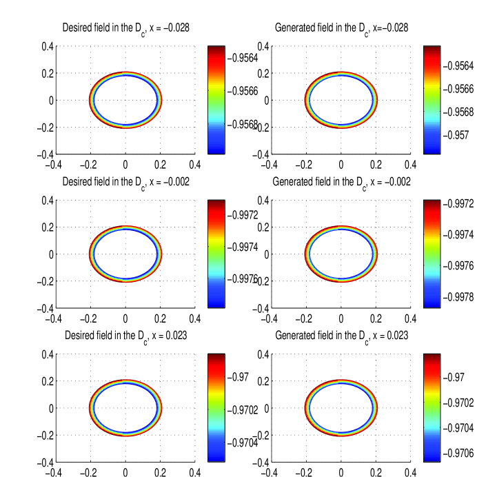
Figure 2: Control of $TM_{10}$ mode

$${\bf E}_{x}(r,\theta,x)=\sum_{m,n}E_{mn}J_{m}(\frac{r\chi_{mn}}{R})cos(m\theta)e^{i\beta_{mn}x},$$ (4.45)

where $E_{mn}$ are coefficients determined by the interrogating field, $J_{m}$ represents the $m$-th order Bessel-$J$ function, $\chi_{mn}$ represents the $n$-th root of $J_{m}$, and $\beta_{mn}=\sqrt{\left(\frac{\omega^{2}}{c^{2}}-\frac{\chi^{2}_{mn}}{R^{2}}\right)}$. For any $m,n$ the term $E_{mn}J_{m}(\frac{r\chi_{mn}}{R})cos(m\theta)e^{i\beta_{mn}x}$ is called the $TM_{mn}$ normal mode and it solves (4.43) with zero boundary data on $\partial B_{R}({\bf 0})$, where $\lambda=\lambda_{mn}=\frac{\omega^{2}}{c^{2}}-\beta_{mn}^{2}=\frac{\chi^{2}_{mn}}{R^{2}}$. Note that we can chose $D_{a^{\prime}}$ and $D_{1}$ in (3.3) and (3.4)so that $\lambda_{mn}$ satisfies the hypothesis of Theorem 3.1. Thus we can use the theoretical results of the previous section. In our numerical results we will show control of the first dominant TM mode with normalized amplitude, i.e., $E_{1x}=J_{0}(\frac{r\chi_{10}}{R})$. For the numerical experiments we considered a radial frequency of 300Mhz, the waveguide $D$ with $R=5$ and the small cylindrical antenna, $D_{a}$, with $\delta=0.05$ and $l=0.3$ is placed in it to control the longitudinal component of the electric field in an incoming $TM_{10}$ mode. The control is numerically showed in a near field cylindrical coaxial shell, $(x,r,\theta)\in D_{c}=[-0.1,0.1]\times[0.13,0.16]\times[0,2\pi]$.

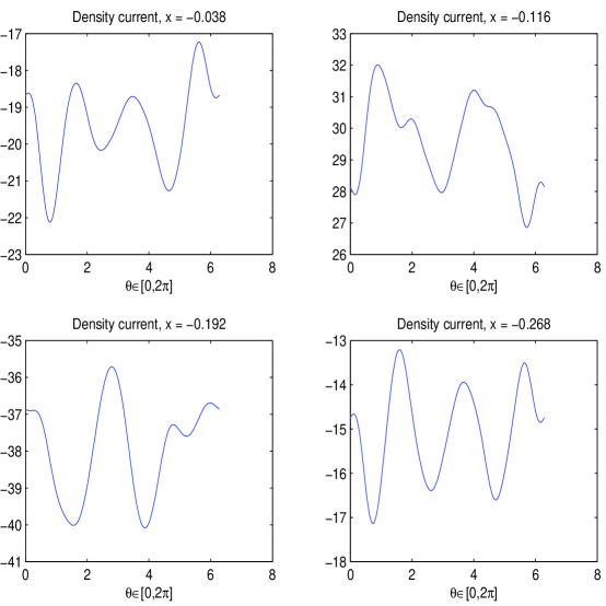
Figure 3: Density current $v_{n}$ as function of $\theta$ for four points on the negative $x$ axis

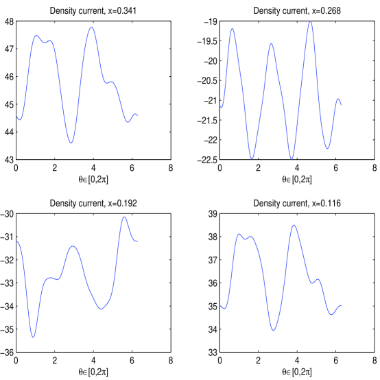
Figure 4: Density current $v_{n}$ as function of $\theta$ for four points on the positive $x$ axis

Figure 2 describes the contour plots of cross-sections of the desired field $-{\bf E}_{x}$ (left column) versus the cross-sections of the field generated by the active antenna ( right column). The three rows in Figure 2 represent the two fields in $D_{c}$ for three cross-section of the antenna, $x=-0.028$, $x=0.002$, $x=0.023$ respectively.

Figure 3 and Figure 4 each describe the density $v_{n}$ introduced in Theorem 3.1 as a function of the angle $\theta\in[0,2\pi]$ for four different values of $x$. We used the Moment Method and Tikhonov regularization scheme to approximate the density function $v_{n}$ on several cross-sections around the center of the antenna.

One can see the high accuracy of the control as well as the limited power budget needed for the desired control which is not the case in the far field schemes (see [52]). In fact the relative $L^{\infty}$ error between the given $E_{1x}$ and the field generated by our active source is of order $O(10^{-4})$ for the dominant mode $TM_{10}$. We only presented the mode with the lowest cutoff frequency but mention that by superposition one will be able to control, in theory, the longitudinal component of any incoming TM field.

5 Feasibility discussion

In this section we will present the analysis of Problem 2. of Question 1. The next result, shows the connection between the class of solutions obtained in the previous section and the main problem stated at Question 1. We have,

Theorem 5.1.

There exists realistic small antennas $D_{a}$ and small magnetic currents ${\bf M}$ to be instantiated on $\partial D_{a}$ such that the electromagnetic field $({\bf E},{\bf H})$ generated will have the property that the longitudinal component of its electric field $E_{xs}$ will satisfy

$$\|u_{n}-E_{xs}\|_{L^{2}(\partial D_{a})}=o(1),\mbox{ as }n\rightarrow\infty,$$ (5.46)

Thus, due to Lemma 5.2, $E_{xs}$ will be very close to $u_{n}$ described in (3.12) and hence achieve the desired control in $D_{c}$ with vanishingly small trace values on the boundary of the waveguide. The surface magnetic current needed for this is characterized by the property that it approaches zero near the ends of the antenna (tappered to zero there) and it satisfies the condition ${\bf M}\cdot\hat{\theta}=E_{b}$ on $\partial D_{a}$ where $\hat{\theta}$ denotes the unit vector in the $\theta$ direction for a cylindrical coordinate system on $D_{a}$.

Proof.

For the proof of Theorem 5.1 we will need the next Lemma which studies the injectivity of the operator $K$ defined at (3.8).

Lemma 5.1.

Assume the conditions of Theorem 3.1. Then the operator $K$ is injective.

Proof.

Consider $w\in L^{2}(\partial D_{a^{\prime}})$ such that $Kw=0$. Then we have

$$\int_{\partial D_{a^{\prime}}}w({\bf y})\frac{\partial\Phi({\bf x},{\bf y})}{\partial\nu_{\bf y}}ds_{\bf y}=0\mbox{ on }\partial D_{1}.$$ (5.47)

From (3.5) and by using the uniqueness of the interior Dirichlet problem we have that

$$\int_{\partial D_{a^{\prime}}}w({\bf y})\frac{\partial\Phi({\bf x},{\bf y})}{\partial\nu_{\bf y}}ds_{\bf y}=0\mbox{ in }{\bar{D}}_{1}.$$ (5.48)

By analytic continuation we get

$$\int_{\partial D_{a^{\prime}}}w({\bf y})\frac{\partial\Phi({\bf x},{\bf y})}{\partial\nu_{\bf y}}ds_{\bf y}=0\mbox{ in }D_{L}\setminus{\bar{D}}_{a^{\prime}}.$$ (5.49)

From (5.49) we have that

$$2\int_{\partial D_{a^{\prime}}}w({\bf y})\frac{\partial\Phi({\bf x},{\bf y})}{\partial\nu_{\bf y}}ds_{\bf y}+w({\bf x})=0\mbox{ on }\partial D_{a^{\prime}}.$$ (5.50)

Next, using our assumption that $-\lambda^{2}$ is not an interior Neumann eigenvalue for $D_{a^{\prime}}$, from (5.50) we obtain $w=0$. ∎

The next Lemma presents a technical regularity result. Since the proof is classical we do not include it here but point out that the result can be obtained by adapting the proof in [18], (Section 3.4).

Lemma 5.2.

Consider $\lambda\in{\mathbb{R}}$ as in Theorem 3.1. Let $f_{e}\in H^{\frac{1}{2}}(\partial D_{a}))$ and let $v_{e}\in C^{2}({\mathbb{R}}^{3}\setminus{\bar{D}_{a}})\cap C({\mathbb{R}}^{3}\setminus D_{a})$ be the unique solution of the following problem,

$$\left\{\begin{array}[]{llll}\Delta v_{e}+\lambda^{2}v_{e}=0\mbox{ in }{\mathbb{R}}^{3}\setminus{\bar{D}}_{a}\vspace{0.15cm}\\ v=f_{e}\mbox{ on }\partial D_{a}\vspace{0.15cm}\\ \displaystyle\left(\frac{x}{|x|},\nabla v_{e}(x))-i\lambda v_{e}(x)\right)=o\left(\frac{1}{|x|}\right),\mbox{ as }|x|\rightarrow\infty,\vspace{0.15cm}\\ \mbox{ uniformly for all directions $\displaystyle\frac{x}{|x|}$. }\end{array}\right.$$ (5.51)

Then, for any given open domain $F\subset{\mathbb{R}}^{3}\setminus{\bar{D}}_{a}$ we have,

$$\|v_{e}\|_{H^{1}(F)}\leq C\|f_{e}\|_{L^{2}(\partial D_{a})},$$

where $C=C(\lambda,\mbox{dist}(\partial D_{a},\partial F))$ with dist function denoting the usual distance between two sets.

We will next propose an antenna geometry together with a strategy for the instantiation of a surface magnetic current ${\bf M}$ satisfying the conditions in Theorem 5.1. Remember that the antenna was assumed to be a coaxial cylinder with round edges and small cross-section area. Thus, consider $\delta_{n}\in C^{2}(-l,l)$, given by $\delta_{n}(x)=\mu_{n}d(x)$ where $\mu_{n}\rightarrow 0$ as $n\rightarrow\infty$, and $d\in C^{2}(-l,l)$ is a smooth cut-off function such that there exists a positive real $0\leq c\leq l$ satisfying,

$$0\leq d=\left\{\begin{array}[]{ll}0,&\mbox{ for }|x|=l\\ 1,&\mbox{ for }x\in(-l+c,l-c)\end{array}\right.,$$ (5.52)

and

$$|d^{\prime}|<C(l,c),\mbox{ for some constant $C(l,c)$ depending only on $l,c$}.$$

Note that, from the definition of $\delta_{n}$ and (5.52) we have

$$|\delta_{n}^{\prime}|\leq C(l,c)\mu_{n},\mbox{ for all }n.$$ (5.53)

Assume the geometry of the antenna to be described by $D_{a}=[-l,l]\times B_{\delta_{n}({\bf 0})}({\bf x})$ for some $l>0\in{\mathbb{R}}^{3}$ for some suitable $n$ large enough. Then ${\bf z}\in\partial D_{a}$ is given by, ${\bf z}=(x,\delta_{n}(x)\cos(\theta),\delta_{n}(x)\sin(\theta))$ for $\theta\in[0,2\pi]$ and $\partial D_{a}$ is a $C^{2}$ smooth surface of rotation with local coordinates $(x,\theta)$ and local tangential vectors $(\frac{d{\bf z}}{dx},\frac{d{\bf z}}{d\theta})$.

The following result is a consequence of Lemma 5.1, classical Fredholm Theory and Tikhonov regularization arguments (see Theorems 3.15,3.17 in [6] and Theorem 4.13 in [5] for example),

Corollary 5.1.

The boundary data $E_{b}$ given in Theorem 3.1 satisfies,

$$\|E_{b}\|_{C^{2}(\partial D_{a})}=\frac{C\sqrt{\mu_{n}}}{s_{n}^{3}}\|u_{n}\|_{L^{2}(\partial D_{a^{\prime}})}\leq\frac{C\sqrt{\mu_{n}}}{s_{n}^{3}\sqrt{\alpha}_{n}}\|E_{xi}\|_{L^{2}(\partial D_{1})},\mbox{ for every }n,$$

where $s_{n}=dist(\partial D_{a^{\prime}},\partial D_{a})$. Observe that for suitable $s_{n}$ (which can be chosen with a suitable choice of $D_{a^{\prime}}$ satisfying (3.4)) and $\alpha_{n}$ we have that

$$\frac{C\sqrt{\mu_{n}}}{s_{n}^{3}\sqrt{\alpha}_{n}}=o(1),\mbox{ as }n\rightarrow\infty.$$ (5.54)

Let ${\bf M}$ be such that ${\bf M}=E_{b}(x,\theta)\hat{\theta}$ where $E_{b}$ is given at (3.40). Note that estimate (5.54) and Corollary 5.1 indicate that,in the limit when $n\rightarrow\infty$, the current ${\bf M}$ will satisfy the continuity equation. Also, note that $v_{n}$ introduced at (3.11) belongs to $C^{\infty}(\partial D_{a})$. From this, Corollary 5.1 we obtain that the vector field ${\bf M}$ will be smooth enough so that for an antenna chosen so that $\lambda$ is not an interior Maxwell eigenvalue the following exterior Maxwell problem problem admits a unique solution (see [6], Section 4.4):

Find ${\bf E}=(E_{x},E_{y},E_{z}),{\bf H}=(B_{x},B_{y},B_{z})\in C^{1}({\mathbb{R}}^{3}\setminus{{\bar{D}}_{a}})\cup C({\mathbb{R}}^{3}\setminus D_{a})$ such that

$$\left\{\begin{array}[]{llll}\nabla\times{\bf E}-i\lambda{\bf H}=0,&\;\nabla\times{\bf H}+i\lambda{\bf E}=0\mbox{ in }{\mathbb{R}}^{3}\setminus{{\bar{D}}_{a}\vspace{0.2cm}}\\ -\nu\times{\bf E}={\bf M},&\mbox{ on }\partial D_{a}\vspace{0.2cm}\\ \left[{\bf H},\frac{{\bf x}}{|{\bf x}|}\right]-{\bf E}=o(\frac{1}{|{\bf x}|}),&\mbox{ as }|{\bf x}|\rightarrow\infty\vspace{0.2cm}\\ \left[{\bf E},\frac{{\bf x}}{|{\bf x}|}\right]+{\bf H}=o(\frac{1}{|{\bf x}|}),&\mbox{ as }|{\bf x}|\rightarrow\infty,\vspace{0.2cm}\end{array}\right.$$ (5.55)

where $\nu$ is the unit exterior normal to $D_{a}$ and where ${\bf M}$ is as above. After simple algebraic manipulations of the boundary condition in (5.55) we observe that the first component of the electric field ${\bf E}$ solution of (5.55), namely $E_{xs}$, is given by,

$$E_{xs}(x,\theta)=E_{b}(x,\theta)\sqrt{(\delta^{\prime}_{n}(x))^{2}+1}-\delta^{\prime}_{n}(x)(E_{z}\sin(\theta)+E_{y}\cos(\theta)).$$ (5.56)

Using (5.56) we obtain

$$\|E_{xs}-E_{b}(x,\theta)\|_{L^{2}(\partial D_{a})} \leq \left\|\frac{(\delta^{\prime}_{n}(x))^{2}E_{b}(x,\theta)}{\sqrt{(\delta^{\prime}_{n}(x))^{2}+1}+1}\right\|_{L^{2}(\partial D_{a})}\!\!\!\!+\|\delta^{\prime}_{n}(x)(E_{z}\sin(\theta)+E_{y}\cos(\theta))\|_{L^{2}(\partial D_{a})}$$ (5.57)

$$\leq o(1),\mbox{ as }n\rightarrow\infty$$

In the second identity of (5.56) we have used (5.53), (5.54) and the fact that $\|E_{z}\|_{L^{2}(\partial D_{a})}$ and $\|E_{y}\|_{L^{2}(\partial D_{a})}$ are $o(1)$ on $\partial D_{a}$ as $n\rightarrow\infty$. Behavior of $\|E_{z}\|_{L^{2}(\partial D_{a})}$ and $\|E_{y}\|_{L^{2}(\partial D_{a})}$ can be obtained by observing that from Corollary 5.1 we have $\|{\bf M}\|_{L^{2}(\partial D_{a})}\rightarrow 0$ on $\partial D_{a}$ as $n\rightarrow\infty$ and then by employing the continuity of the solution operator for problem (5.55) with $L^{2}$ boundary data (see [62], Section 6.3). In fact this behavior can also be obtained from the observation that based on our strategy of a possible instantiation presented below we need small conduction currents to excite the small magnetic current ${\bf M}$ and thus the electric field will be very small on the surface of the antenna.

Next by using Lemma 5.2 we obtain that for suitable chosen $\alpha_{n}$ there exist $n$ large enough such that for any sub-domain $F$, $F\subsetneq{\mathbb{R}}^{3}\setminus{\bar{D}}_{a}$, we have

$$\|E_{xs}-E_{b}\|_{H^{1}(F)}\leq Co((\mu_{n})^{\frac{1}{2}}),\mbox{ as }n\rightarrow\infty.$$ (5.58)

where $C=C(\lambda,\mbox{dist}(\partial F,\partial D_{a}))$ and we have used that $|\partial D_{a}|=O(\mu_{n})$.

Thus, we showed that for large enough $n$, an antenna with the geometry described above and with a magnetic current ${\bf M}$ excited on its surface as indicated above generates an electromagnetic field ${\bf E},{\bf H}$, solution of (5.55), which satisfies the properties of Theorem 5.1. ∎

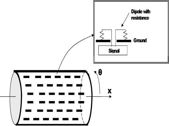
Figure 5: The proposed antenna is a closely spaced array on a metallic cylinder with small diameter. Each dipole (as shown in the inset) is resistively loaded to the metallic cylinder so the dipole currents are spatially constant across the length of the dipole.

The central purpose of this paper is to study the process whereby electromagnetic fields can be nulled or otherwise controlled locally in the sinusoidal or harmonic case. The infinite circular waveguide was studied because of the stability of its modes and their simplicity relative to other structures including far field regimes.

However, there also is a practical interest. On one hand, devices to switch signals from one waveguide to another in a branching configuration are commercially available and based on our review of the literature and practice these devices appear to be mechanical in nature. Additionally, there has also been consideration of suppression of unwanted modes ( references [63],[64]). Thus, this research on suppression of longitudinal modes in a cylindrical waveguide may have some interest to microwave engineers for mode suppression or switching. This leads to a consideration of physical realization of the control activity specified by the analysis presented above.

We will now discuss about a possible instantiation of this antenna (see Figure 5). As discussed above, the sufficient condition that the longitudinal component of the electric field of the antenna (modeled as magnetic surface currents ${\bf M}$) has the desired control properties in the near field control region $D_{c}$ with vanishingly small values on $\partial D$, is that the inner product of the local magnetic current $M(x,\theta)$ with the unit vector $\hat{\theta}$ equals $E_{b}$ described (3.13). Therefore from the point of view of realizing this nulling antenna this sufficient condition must be instantiated. The complexity of the problem is well illustrated by reference to Figures 3 and 4 above. It is evident that the field control is made possible in this analysis by a boundary density function that is a function of distance along the longitudinal axis of the central antenna, and is also an independent function of the angle theta around the axis. The controlled modes are modes that are parallel to the antenna surface. In the electromagnetic case, the question arises of how this would be accomplished.

In the case of exterior scattering problems, Kersten ([65]) has shown that boundary densities may be replaced for a set of interior electric and magnetic dipoles while preserving the exterior scattered field (see also [66] ). While an argument equivalent in rigor is not known to us concerning antenna field generation by secondary sources, the method of auxiliary sources has been used effectively in the assessment of antenna radiation properties including far field structures and input impedance ( [67], [68], [69]). Thus, we have been encouraged to consider an electromagnetic physical realization of the complex radiating structure called for in the analysis described above. Also, perhaps most importantly, Theorem 5.1 translates the Helmholtz control results and calculations of Sections 2, 3 , and 4 into electromagnetic terms indicating the existence of a suitable antenna.

A candidate structure which we are studying to realize the requirements of this analysis is an array of very small horizontally oriented dipoles supported on a conductive surface as diagrammed in the Figure 5. Since the dipoles are resistively loaded (that is, there is a conductive path to the cylindrical ground plane), a spatially constant, temporally oscillating current can be maintained in the metallic arms of each dipole using the signal generator. Thus, this arrangement permits a varying current with theta and with the linear dimension x. This is an example of a dense array, an antenna design of present interest ([70]). This surface current developed by the array is such that it is proportional to the electric field parallel to the cylinder (a longitudinal) mode, and thus the current acts as the desired magnetic current density.

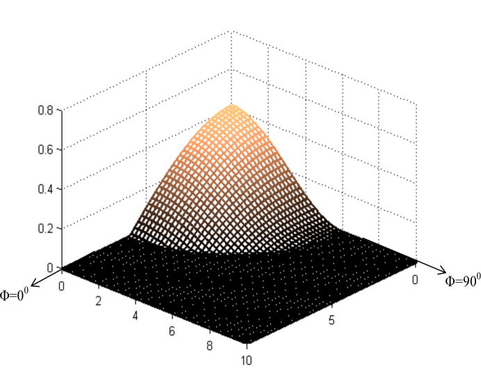
Figure 6: This figure shows an estimate of the dipole field amplitude in the direction parallel to the cylindrical array structure as a function of elevation (polar) angle and azimuth angle around the horizontal dipole (in the figure placed in the north corner of the $x,y$ plane along the $\Phi=0\textdegree$ axis) . Each plane in this figure orthogonal to the $x,y$ plane and including the z axis, provides a view of the field amplitude with elevation angle at a given azimuth. The $\Phi=0\textdegree$ plane corresponds to the zero azimuth angle.

Each dipole produces a field that has a component that is directed radially (orthogonal to the cylinder surface), but most importantly, as stated in the paragraph above, there is a component that is parallel to the cylindrical surface. The field structure of a horizontal dipole over a perfect ground plane is shown in Figure 6 following Balanis’ development([71]). This field structure approximates the field of the dipole mounted on a cylindrical metallic structure as shown above. Combining these field structures using array principles results (treating each field structure as a basis function) in an approximation to the effect of the controlling current density specified in this Section.

References

- [1] A. Alu and N. Engheta, Plasmonic and metamaterial cloaking: physical mechanism and potentials, J. Opt. A: Pure Appl. Opt, 10, (2008).
- [2] H. Brezis, Analyse functionnelle. Theorie et applications, Dunod, Paris, France, 2nd ed., (1999).
- [3] H. Chen and C. Chan, Acoustic cloaking and transformation acoustics, J. Phys. D: Appl. Phys., 43, (2010).
- [4] H. Chen, C. T. Chan, and P. Sheng, Transformation optics and metamaterials, Nature Materials, 9, pp. 387–396, (2010).
- [5] D. Colton and R. Kress, Inverse Acoustic and Electromagnetic Scattering Theory, Springer-Verlag, New York, (1998).
- [6] D. Colton and R. Kress, Integral Equation Methods in scattering Theory, Pure & Applied Math., Wiley Interscience, New York, (1983).
- [7] S. A. Cummer, B.-I. Popa, D. Schurig, D. R. Smith, J. Pendry, M. Rahm, A. Starr, Scattering theory derivation of a 3d acoustic cloaking shell, Phys. Rev. Lett., 100, (2008).
- [8] A. Greenleaf, Y. Kurylev, M. Lassas, G. Uhlmann, Invisibility and inverse problems, Bull. Amer. Math. Soc., 46, pp. 55–97, (2009).
- [9] A. Greenleaf, M. Lassas, and G. Uhlmann, Anisotropic conductivities that cannot be detected by eit, Physiol. Meas., 24, pp. 413–419, (2003).
- [10] A. Greenleaf, Y. Kurylev, M. Lassas, G. Uhlmann, Full-wave invisibility of active devices at all frequencies, Comm. Math. Phys., vol. 275, 749-789, (2007).
- [11] A. Greenleaf, M. Lassas, G. Uhlmann, On nonuniqueness for Calderón’s inverse problem, Mathematical Research Letters, vol. 10, 685-693, (2003).
- [12] F. Guevara Vasquez, G. W. Milton, D. Onofrei, P. Seppecher, Transformation elastodynamics and active exterior acoustic cloaking, Acoustic metamaterials: Negative refraction, imaging, lensing and cloaking, arXiv:1105.1221, (2011).
- [13] F. Guevara Vasquez, G. W. Milton, and D. Onofrei, Active exterior cloaking, Phys. Rev. Lett., 103, (2009).
- [14] , Broadband exterior cloaking, Optics Express, 17, pp. 14800–14805, (2009).
- [15] , Exterior cloaking with active sources in two dimensional acoustics, accepted Wave Motion, arXiv:1009.2038, (2011).
- [16] A. Kirsch, An Introduction to the Mathematical Theory of Inverse Problems, Springer-Verlag, New York, (1996).
- [17] R. Kohn, D. Onofrei, M. Vogelius, and M. Weinstein, Cloaking via change of variables for the helmholtz equation at fixed frequency, Comm. Pure. Appl. Math., 63, pp. 973–1016, (2000).
- [18] R. Kress, Linear Integral Equations, Applied Mathematical Sciences, Springer-Verlag, New York, 2nd ed., (1999).
- [19] Y. Lai, H. Chen, Z.-Q. Zhang, and C. T. Chan, Complementary media invisibility cloak that cloaks objects at a distance outside the cloaking shell, Phys. Rev. Lett., 102, (2009).
- [20] U. Leonhardt, Notes on conformal invisibility devices, New J. Phys., 8, p. 118, (2006).
- [21] , Optical conformal mapping, Science, 312, pp. 1777–1780, (2006).
- [22] D. A. B. Miller, On perfect cloaking, Opt. Express, 14, pp. 12457–12466, (2006).
- [23] G. W. Milton and N.-A. P. Nicorovici, On the cloaking effects associated with anomalous localized resonance, Proc. R. Soc. Lon. Ser. A. Math. Phys. Sci., 462, pp. 3027–3059, (2006).
- [24] G. W. Milton, N.-A. P. Nicorovici, R. C. McPhedran, K. Cherednichenko, and Z. Jacob, Solutions in folded geometries, and associated cloaking due to anomalous resonance, New J. Phys., 10, (2008).
- [25] N.-A. P. Nicorovici, G. Milton, R. C. McPhedran, and L. C. Botten, Quasistatic cloaking of two-dimensional polarizable discrete systems by anomalous resonance, Opt. Express, 15, pp. 6314–6323, (2007).
- [26] J. B. Pendry, D. Schurig, and D. R. Smith, Controlling electromagnetic fields, Science, 312, pp. 1780–1782, (2006).
- [27] I. I. Smolyaninov, V. N. Smolyaninova, A. V. Kildishev, and V. M. Shalaev, Anisotropic metamaterials emulated by tapered waveguides: Application to optical cloaking, Phys. Rev. Lett., 103, (2009).
- [28] Hoai-Minh Nguyen, Approximate cloaking for the Helmholtz equation via transformation optics and consequences for perfect cloaking, to appear in Comm. Pure Appl. Math , Comm. Pure. Appl. Math., Volume 65, Issue 2, pages 155–186, (2012).
- [29] H. Y. Liu, Virtual reshaping and invisibility in obstacle scattering, Inverse Problems, 25, 045006, (2009).
- [30] Hongyu Liu, Hongpeng Sun, Enhanced Near-cloak by FSH Lining, online at arXiv:1110.0752, (2011).
- [31] Hongyu Liu, Ting Zhou, On Approximate Electromagnetic Cloaking by Transformation Media , SIAM J. Appl. Math., 71, pp. 218–241, (2011).
- [32] L. S. Dolin, On a possibility of comparing three-dimensional electromagnetic systems with inhomogeneous filling, Izv. Vyssh. Uchebn. Zaved. Radiofiz. 4, 964, (1961).
- [33] E. J. Post, Formal structure of electromagnetics, North-Holland (1962).
- [34] M. Lax and D. F. Nelson, “Maxwell equations in material form,” Phys. Rev. B 13, 1777, (1976).
- [35] H. Ammari, Hyeonbae Kang, Hyundae Lee, Mikyoung Lim,Enhancement of near-cloaking. Part II: the Helmholtz equation, To appear in Communications in Mathematical Physics, (2012).
- [36] H. Ammari, J. Garnier, V. Jugnon, H. Kang, H. Lee, and M. Lim, Enhancement of near-cloaking. Part III: numerical simulations, statistical stability, and related questions. To appear in Contemporary Mathematics (2012).
- [37] H. Ammari, H. Kang, H. Lee, and M. Lim, Enhancement of near-cloaking using generalized polarization tensors vanishing structures. Part I: The conductivity problem. to appear in Communications in Mathematical Physics (2012).
- [38] J. Valentine, Z. Shuang, T. Zentgraf, Z. Xiang Development of Bulk Optical Negative Index Fishnet Metamaterials: Achieving a Low-Loss and Broadband Response Through Coupling, Proceedings of the IEEE, Vol. 99, Iss. 10 pp. 1682 - 1690, (2011).
- [39] Allan Greenleaf, Yaroslav Kurylev, Matti Lassas, Gunther Uhlmann, Schrodinger’s Hat: Electromagnetic, acoustic and quantum amplifiers via transformation optics, online at arxiv.org: arXiv:1107.4685v1, 2011.
- [40] N. Peake, D.G. Crighton, Active control of sound, Annu. Rev. Fluid Mech., vol.32, 137-164, (2000).
- [41] S.J. Elliot, P.A. Nelson, The active control of sound, Electronics and Comm. Engineering Journal, August, (1990).
- [42] J. Loncaric, V.S. Ryaben’kii, S.V. Tsynkov, Active shielding and control of environmental noise, technical report, NASA/CR-2000-209862, ICASE Report No. 2000-9, (2000).
- [43] J. Loncaric, S.V. Tsynkov, Quadratic optimization in the problems of active control of sound, Appl. NUm. Math., vol. 52, 381-400, (2005).
- [44] A.W. Peterson, S.V. Tsynkov, Active control of sound for composite regions, SIAM J. Appl. Math, vol. 67, Iss. 6, pp 1582-1609, (2007).
- [45] C.R. Fuller, A.H. von Flotow, Active control of sound and vibration, IEEE, (1995).
- [46] P. Leug, Process of silencing sound oscillations, U.S. patent no. 2043416, (1936).
- [47] H.F. Olson, E.G. May, Electronic sound absorber, J. Acad. Soc. America, vol. 25, pp. 1130-1136, (1953).
- [48] A. Greenleaf, Y. Kurylev, M. Lassas, G. Uhlmann, Cloaking a Sensor via Transformation Optics, Physical Review E 83, 016603 (2011).
- [49] G. Castaldi, I. Gallina, V. Galdi, A. Alu, N. Engheta, Power scattering and absorption mediated by cloak/anti-cloak interactions: A transformation-optics route towards invisible sensors, JOSA B, Vol. 27, Iss. 10, pp. 2132-2140, (2010).
- [50] H. H. Zheng, J. J. Xiao, Y. Lai, C. T. Chan Exterior optical cloaking and illusions by using active sources: A boundary element perspective, Phys. Rev. B, Vol. 81, Issue 19, (2010).
- [51] Y. Lai, Jack Ng, H. Chen, D. Han, J. Xiao, Z. Zhang, C. T. Chan, Illusion Optics: The Optical Transformation of an Object into Another Object, Phys. Rev. Lett. 102, 253902 (2009).
- [52] A. N. Norris, F. A. Amirkulova, W. J. Parnell, ”Source amplitudes for active exterior cloaking”, arXiv:1207.4801, (2012).
- [53] D. Onofrei, On the active manipulation of fields and applications. I - The Quasistatic regime, Inverse problems, Inverse Problems Vol. 28, No. 10, (2012).
- [54] K.N. Makrakis, A.G. Ramm, Scattering by obstacles in acoustic waveguides, Spectral and scattering theory, Plenum publishers, New York, (ed. A.G.Ramm) pp. 89-110., (1998).
- [55] D. Onofrei, R. Albanese, Synthesis of antennas in cylindrical waveguides with prescribed longitudinal components of their electric fields, in preparation.
- [56] J. Du, S. Liu, Z. Lin, Broadband Optical Cloak and Illusion Created by the Low Order Active Sources, Opt Express., Apr 9, 20(8):8608-17, (2012).
- [57] M. Selvanayagam, G. V. Eleftheriades, An Active Electromagnetic Cloak Using the Equivalence Principle IEEE Ant. and Wireless Prop. Lett., vol. 11, (2012).
- [58] M. Selvanayagam, G. V. Eleftheriades, Experimental Demonstration of Active Electromaagnetic Cloaking, Phys. Rev. X, vol. 3, Iss. 4, (2013)
- [59] Qian Ma, Zhong Lei Mei, Shou Kui Zhu, and Tian Yu Jin, Experiments on Active Cloaking and Illusion for Laplace Equation, Phys. Rev. Lett., vol. 111, Iss. 17, (2013)
- [60] A. Kirsch, The Robin problem for the Helmholtz equation as a singular perturbation problem, Numer. Funct. Anal. And Optimiz., 8(1), 1-20, (1985).
- [61] Constantine A. Balanis, Antenna Theory: Analysis and Design, John Wiley & Son Inc., 3rd edition, (2005)
- [62] Thomas S. Angell, Andreas Kirsch, Optimization Methods in Electromagnetic Radiation, Springer Monographs in Mathematics, (2004).
- [63] R. Garg, K. C. Gupta, Suppression of Slot Mode in Slotted Waveguide Antennas, IEEE Transactions on Antennas and Propagation, pages 731-732, 1975.
- [64] C. Q. Jiao, Selective Suppression Of Electromagnetic Modes In A Rectangular Waveguide By Using Distributed Wall Losses, Progress In Electromagnetics Research Letters, Vol. 22, 119-128, (2011).
- [65] H. Kersten Die Losung der Maxwellschen Gleichungen durch vollstandige Flachenfeldsysteme, Math. Meth. Apl. Sci, 7, 40-45, (1985).
- [66] T. Wriedt, A. Doicu Formulations of the extended boundary condition method for three-dimensional scattering using the method of discrete sources, Jour. Modern Optics, 1998, VOL. 45, NO. 1, 199 - 213
- [67] S. G. Diamanis, A. P. Orfanidis, G. A. Kyriacou, J. N. Shalos, Horn Antennas Analysis Using a Hybrid Mode Matching-Auxiliary Sources Technique, Progress in Electromagnetic Research Symposium, Pisa, Italy, March 28-31, pages 457-460, (2004)
- [68] R. S. Zaridze, I.M. Petoev, V.A. Tabatadze, B.V. Poniava The Method Of Auxiliary Sources For Antenna Synthesis Problems, DIPED- Proceedings, pages 13-19, (2013)
- [69] G. Fikioris, On Two Types of Convergence in the Method of Auxiliary Sources, IEEE Transactions On Antennas And Propagation, VOL. 54, NO. 7, JULY ???
- [70] J. D. Krieger, Chen-Pang Yeang, G.W. Wornell, Dense Delta-Sigma Phased Arrays, IEEE Transactions On Antennas And Propagation, VOL. 61, NO. 4, April (2013)
- [71] C. A. Balanis, Antenna Theory; Analysis and Design, John Wiley and Sons, New York, 1st Edition, 1551-1554.