Hallucinating Optimal High-Dimensional Subspaces

Abstract

Linear subspace representations of appearance variation are pervasive in computer vision. This paper addresses the problem of robustly matching such subspaces (computing the similarity between them) when they are used to describe the scope of variations within sets of images of different (possibly greatly so) scales. A naïve solution of projecting the low-scale subspace into the high-scale image space is described first and subsequently shown to be inadequate, especially at large scale discrepancies. A successful approach is proposed instead. It consists of (i) an interpolated projection of the low-scale subspace into the high-scale space, which is followed by (ii) a rotation of this initial estimate within the bounds of the imposed “downsampling constraint”. The optimal rotation is found in the closed-form which best aligns the high-scale reconstruction of the low-scale subspace with the reference it is compared to. The method is evaluated on the problem of matching sets of (i) face appearances under varying illumination and (ii) object appearances under varying viewpoint, using two large data sets. In comparison to the naïve matching, the proposed algorithm is shown to greatly increase the separation of between-class and within-class similarities, as well as produce far more meaningful modes of common appearance on which the match score is based.

1 Introduction

One of the most commonly encountered problems in computer vision is that of matching appearance. Whether it is images of local features [1], views of objects [2] or faces [3], textures [4] or rectified planar structures (buildings, paintings) [5], the task of comparing appearances is virtually unavoidable in a modern computer vision application. A particularly interesting and increasingly important instance of this task concerns the matching of sets of appearance images, each set containing examples of variation corresponding to a single class.

A ubiquitous representation of appearance variation within a class is by a linear subspace [6, 7]. The most basic argument for the linear subspace representation can be made by observing that in practice the appearance of interest is constrained to a small part of the image space. Domain-specific information may restrict this even further e.g. for Lambertian surfaces seen from a fixed viewpoint but under variable illumination [8, 9, 10] or smooth objects across changing pose [11, 12]. What is more, linear subspace models are also attractive for their low storage demands – they are inherently compact and can be learnt incrementally [13, 14, 15, 16, 17, 18]. Indeed, throughout this paper it is assumed that the original data from which subspaces are estimated is not available.

A problem which arises when trying to match two subspaces – each representing certain appearance variation – and which has not as of yet received due consideration in the literature, is that of matching subspaces embedded in different image spaces, that is, corresponding to image sets of different scales. This is a frequent occurrence: an object one wishes to recognize may appear larger or smaller in an image depending on its distance, just as a face may, depending on the person’s height and positioning relative to the camera. In most matching problems in the computer vision literature, this issue is overlooked. Here it is addressed in detail and shown that a naïve approach to normalizing for scale in subspaces results in inadequate matching performance. Thus, a method is proposed which without any assumptions on the nature of appearance that the subspaces represent, constructs an optimal hypothesis for a high-resolution reconstruction of the subspace corresponding to low-resolution data.

In the next section, a brief overview of the linear subspace representation is given first, followed by a description of the aforementioned naïve scale normalization. The proposed solution is described in this section as well. In Section 3 the two approaches are compared empirically and the results analyzed in detail. The main contribution and conclusions of the paper are summarized in Section 4.

2 Matching Subspaces across Scale

Consider a set $X\subset\mathbb{R}^{d}$ containing vectors which represent rasterized images:

$$X=\big{\{}\mathbf{x}_{1},\ldots,\mathbf{x}_{N}\big{\}}$$ (1)

where $d$ is the number of pixels in each image. It is assumed that all of the images represented by members of $X$ have the same aspect ratio, so that the same indices of different vectors correspond spatially to the same pixel location. A common representation of appearance variation described by $X$ is by a linear subspace of dimension $D$, where usually it is the case that $D\ll d$. If $\mathbf{m}_{X}$ is the estimate of the mean of the samples in $X$:

$$\mathbf{m}_{X} =\frac{1}{N}\sum_{i=1}^{N}\mathbf{x}_{i},$$ (2)

then $\mathbf{B}_{X}\in\mathbb{R}^{d\times D}$, a matrix with columns consisting of orthonormal basis vectors spanning the $D$-dimensional linear subspace embedded in a $d$-dimensional image space, can be computed from the corresponding covariance matrix $\mathbf{C}_{X}$:

$$\mathbf{C}_{X} =\frac{1}{N-1}\sum_{i=1}^{N}\big{(}\mathbf{x}_{i}-\mathbf{m}_{X}\big{)}\big{(}\mathbf{x}_{i}-\mathbf{m}_{X}\big{)}^{T}.$$ (3)

Specifically, an insightful interpretation of $\mathbf{B}_{X}$ is as the row and column space basis of the best rank-$D$ approximation to $\mathbf{C}_{X}$:

$$\mathbf{B}_{X}=\arg\min_{\scriptsize\begin{array}[]{c}\mathbf{B}\in\mathbb{R}^{d\times D}\\ \mathbf{B}^{T}\mathbf{B}=I\end{array}}\min_{\scriptsize\begin{array}[]{c}\Lambda\in\mathbb{R}^{D\times D}\\ \Lambda_{ij}=0,i\neq j\end{array}}{\big{\|}~{}\mathbf{C}_{X}-\mathbf{B}~{}\Lambda~{}\mathbf{B}^{T}~{}\big{\|}_{F}}^{2},$$ (8)

where $\|.\|_{F}$ is the Frobenius norm of a matrix.

2.1 The “Naïve Solution”

Let $\mathbf{B}_{X}\in\mathbb{R}^{d_{l}\times D}$ and $\mathbf{B}_{Y}\in\mathbb{R}^{d_{h}\times D}$ be two basis vectors matrices corresponding to appearance variations of image sets containing images with $d_{l}$ and $d_{h}$ pixels respectively. Without loss of generality, let also $d_{l}<d_{h}$. As before, here it is assumed that all images both within each set, as well as across the two sets, are of the same aspect ratio. Thus, we wish to compute the similarity of sets represented by orthonormal basis matrices $\mathbf{B}_{X}$ and $\mathbf{B}_{Y}$.

Subspaces spanned by the columns of $\mathbf{B}_{X}$ and $\mathbf{B}_{Y}$ cannot be compared directly as they are embedded in different image spaces. Instead, let us model the process of an isotropic downsampling of a $d_{h}$-pixel image down to $d_{l}$ pixels with a linear projection realized though a projection matrix $\mathbf{P}\in\mathbb{R}^{d_{l}\times d_{h}}$. In other words, for a low-resolution image set $X\subset\mathbb{R}^{d_{l}}$:

$$X=\big{\{}\mathbf{x}_{1},\ldots,\mathbf{x}_{N}\big{\}}$$ (9)

there is a high-resolution set $X^{*}\subset\mathbb{R}^{d_{h}}$, such that:

$$X^{*}=\bigg{\{}\mathbf{x}_{i}^{*}~{}|~{}\mathbf{x}_{i}=\mathbf{P}~{}\mathbf{x}_{i}^{*}~{};~{}i=1,\ldots,N\bigg{\}}.$$ (10)

The form of the projection matrix depends on (i) the projection model employed (e.g. bilinear, bicubic etc.) and (ii) the dimensions of high and low scale images; see Figure 1 for an illustration.

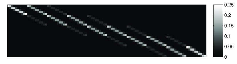
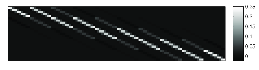
Figure 1: The projection matrix $\mathbf{P}\in\mathbb{R}^{25\times 100}$ modelling the process of downsampling a $10\times 10$ pixel image to $5\times 5$ pixels, using (a) bilinear and (b) bicubic projection models, shown as an image. For the interpretation of image intensities see the associated grey level scales on the right.

Under the assumption of a linear projection model, the least-square error reconstruction of the high-dimensional data can be achieved with a linear projection as well, in this case by $\mathbf{P}_{R}$ which can be computed as:

$$\mathbf{P}_{R}=\mathbf{P}^{T}~{}\left(\mathbf{P}~{}\mathbf{P}^{T}\right)^{-1}.$$ (11)

Since it is assumed that the original data from which $\mathbf{B}_{X}$ was estimated is not available, an estimate of the subspace corresponding to $X^{*}$ can be computed by re-projecting each of the basis vectors (columns) of $\mathbf{B}_{X}$ into $\mathbb{R}^{d_{h}}$:

$$\tilde{\mathbf{B}}^{*}_{X}=\mathbf{P}_{R}~{}\mathbf{B}_{X}.$$ (12)

Note that in general $\tilde{\mathbf{B}}^{*}_{X}$ is not an orthonormal matrix i.e. ${{}\tilde{\mathbf{B}}_{X}^{*}}^{T}~{}\tilde{\mathbf{B}}^{*}_{X}\neq\mathbf{I}$. Thus, after re-projecting the subspace basis, it is orthogonalized using the Householder transformation [19], producing a high-dimensional subspace basis estimate $\mathbf{B}^{*}_{X}$ which can be compared directly with $\mathbf{B}_{Y}$.

2.1.1 Limitations of the Naïve Solution

The process of downsampling an image inherently causes a loss of information. In re-projecting the subspace basis vectors, information gaps are “filled in” through interpolation. This has the effect of constraining the spectrum of variation in the high-dimensional reconstructions to the bandwidth of the low-dimensional data. Compared to the genuine high-resolution images, the reconstructions are void of high frequency detail which usually plays a crucial role in discriminative problems.

2.2 Proposed Solution

We seek a constrained correction to the subspace basis $\mathbf{B}^{*}_{X}$. To this end, consider a vector $\mathbf{x}^{*}_{i}$ in the high-dimensional image space $\mathbb{R}^{d_{h}}$, which when downsampled maps onto $\mathbf{x}_{i}$ in $\mathbb{R}^{d_{l}}$. As before, this is modelled as a linear projection effected by a projection matrix $\mathbf{P}$:

$$\mathbf{x}_{i}=\mathbf{P}~{}\mathbf{x}^{*}_{i}.$$ (13)

Writing the reconstruction of $\mathbf{x}^{*}_{i}$, computed as described in the previous section, as $\mathbf{x}^{*}_{i}+\mathbf{c}_{i}$, it has to hold:

$$\mathbf{x}_{i}=\mathbf{P}~{}\big{(}\mathbf{x}^{*}_{i}+\mathbf{c}_{i}\big{)},$$ (14)

or, equivalently:

$$\mathbf{0}=\mathbf{P}~{}\mathbf{c}_{i},$$ (15)

In other words, the correction term $\mathbf{c}_{i}$ has to lie in the nullspace of $\mathbf{P}$. Let $\mathbf{B}_{c}$ be a matrix of basis vectors spanning the nullspace which, given its meaning in the proposed framework, will henceforth be referred to as the ambiguity constraint subspace. Then the actual appearance in the high-dimensional image space corresponding to the subspace $\mathbf{B}_{X}\in\mathbb{R}^{d_{l}\times D}$ is not spanned by the $D$ columns of $\mathbf{B}^{*}_{X}$ but rather some $D$ orthogonal directions in the span of the columns of $\big{[}\mathbf{B}^{*}_{X}~{}|~{}\mathbf{B}_{c}\big{]}$, as illustrated in Figure 2.

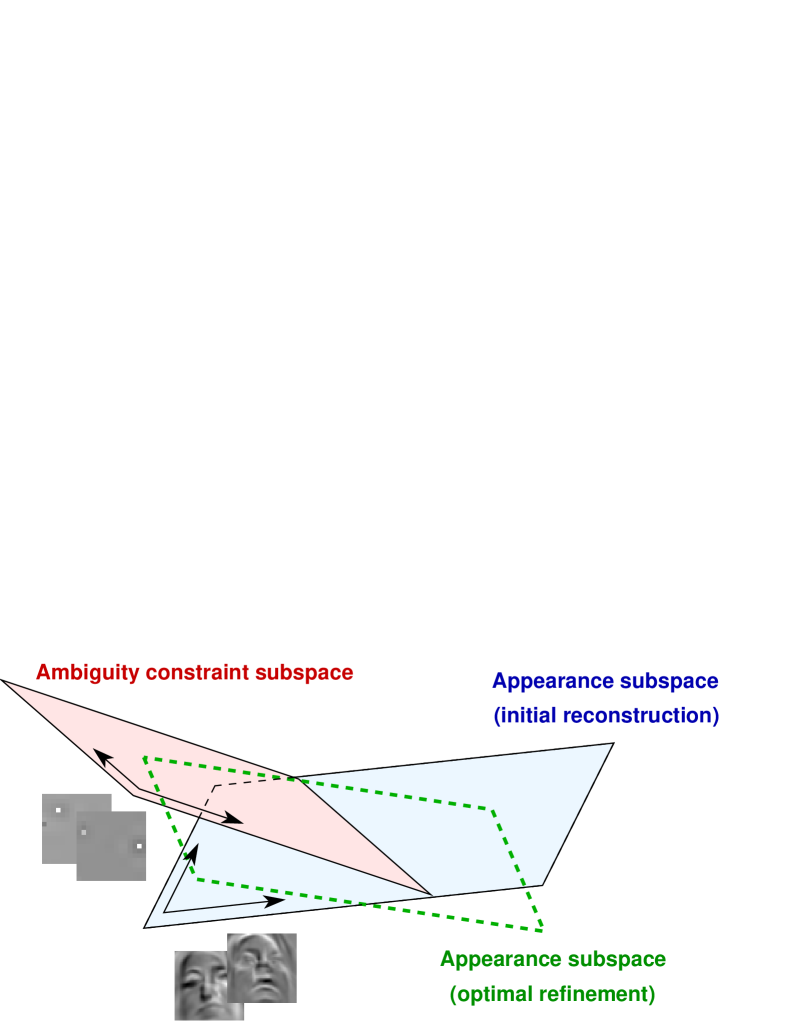
Figure 2: A conceptual illustration of the main idea: the initial reconstruction of the class subspace in the high dimensional image space is refined through rotation within the constraints of the ambiguity constraint subspace.

Let $\mathbf{B}_{Xc}$ be a matrix of orthonormal basis vectors computed by orthogonalizing $\big{[}\mathbf{B}^{*}_{X}~{}|~{}\mathbf{B}_{c}\big{]}$:

$$\mathbf{B}_{Xc}=\text{orth}\big{(}\big{[}\mathbf{B}^{*}_{X}~{}|~{}\mathbf{B}_{c}\big{]}\big{)}$$ (16)

Then we seek a matrix $\mathbf{T}\in\mathbb{R}^{(D+d_{h}-d_{l})\times D}$ which makes the optimal choice of $D$ directions from the span of $\mathbf{B}_{Xc}$:

$$\mathbf{B}_{Xc}~{}\mathbf{T}=\mathbf{B}_{Xc}~{}\bigg{[}~{}\mathbf{t}_{1}~{}|~{}\mathbf{t}_{2}~{}|~{}\ldots~{}|~{}\mathbf{t}_{D}~{}\bigg{]}.$$ (17)

Here the optimal choice of $\mathbf{T}$ is defined as the one that best aligns the reconstructed subspace with the subspace it is compared with, i.e. $\mathbf{B}_{Y}$. The matrix $\mathbf{T}$ can be constructed recursively, so let us consider how its first column $\mathbf{t}_{1}$ can be computed. The optimal alignment criterion can be restated as:

$$\mathbf{t}_{1} =\text{arg}\max_{\mathbf{t}^{\prime}_{1}}\max_{\mathbf{a}}\frac{\big{(}\mathbf{B}_{Y}~{}\mathbf{a}\big{)}\cdot\big{(}\mathbf{B}_{Xc}~{}\mathbf{t}^{\prime}_{1}\big{)}}{\|\mathbf{a}\|~{}\|\mathbf{t}^{\prime}_{1}\|}$$ (18)

Rewriting the right-hand side:

$$\mathbf{t}_{1} =\text{arg}\max_{\mathbf{t}^{\prime}_{1}}\max_{\mathbf{a}}\frac{\big{(}\mathbf{B}_{Y}~{}\mathbf{a}\big{)}\cdot\big{(}\mathbf{B}_{Xc}~{}\mathbf{t}^{\prime}_{1}\big{)}}{\|\mathbf{a}\|~{}\|\mathbf{\mathbf{t}^{\prime}_{1}}\|}=$$ (19)

$$=\text{arg}\max_{\mathbf{t}^{\prime}_{1}}\max_{\mathbf{a}}\frac{\mathbf{a}^{T}}{\|\mathbf{a}\|}~{}{\mathbf{B}_{Y}}^{T}~{}\mathbf{B}_{Xc}~{}\frac{\mathbf{t}^{\prime}_{1}}{\|\mathbf{\mathbf{t}^{\prime}_{1}}\|}=$$ (20)

$$=\text{arg}\max_{\mathbf{t}^{\prime}_{1}}\max_{\mathbf{a}}\frac{\mathbf{a}^{T}}{\|\mathbf{a}\|}~{}\mathbf{U}~{}\Sigma~{}{\mathbf{V}}^{T}~{}\frac{\mathbf{t}^{\prime}_{1}}{\|\mathbf{\mathbf{t}^{\prime}_{1}}\|},$$ (21)

where:

$${\mathbf{B}_{Y}}^{T}~{} \mathbf{B}_{Xc}=$$

$$\overbrace{\bigg{[}~{}\mathbf{u}_{1}~{}|~{}\ldots~{}|~{}\mathbf{u}_{D}~{}\bigg{]}}^{\mathbf{U}}~{}\overbrace{\left[\begin{array}[]{cccccc}~{}~{}\sigma_{1}{}{}&0&\ldots&0&\ldots&0\\ 0&~{}~{}\sigma_{2}{}{}&\ldots&0&\ldots&0\\ \vdots&\vdots&~{}~{}\ddots{}{}&\vdots&\ldots&0\\ 0&0&\ldots&~{}~{}\sigma_{D}{}{}&\ldots&0\\ \end{array}\right]}^{\Sigma}~{}\overbrace{\bigg{[}~{}\mathbf{v}_{1}~{}|~{}\ldots~{}|~{}\mathbf{v}_{D+d_{h}-d_{l}}~{}\bigg{]}^{T}}^{\mathbf{V}^{T}},$$ (26)

is the Singular Value Decomposition (SVD) of ${\mathbf{B}_{Y}}^{T}~{}\mathbf{B}_{Xc}$ and $\sigma_{1}\geq\sigma_{2}\geq\ldots\geq\sigma_{D}$. Then, from the right-hand side in Equation (21), by inspection the optimal directions of $\mathbf{a}$ and $\mathbf{t}^{\prime}_{1}$ are, respectively, the first SVD “output” direction $\mathbf{u}_{1}$ and the first SVD “input” direction, i.e. $\mathbf{a}=\mathbf{u}_{1}$, and $\mathbf{t}_{1}=\mathbf{v}_{1}$. The same process can be used to infer the remaining columns of $\mathbf{T}$, the $i$-th one being $\mathbf{t}_{i}=\mathbf{v}_{i}$.

Thus, the optimal reconstruction $\mathbf{B}^{\prime}_{X}$ of $\mathbf{B}_{X}$ in the high-dimensional space, obtained by the constrained rotation of the naïve estimate $\mathbf{B}^{*}_{X}$, is given by the orthonormal basis matrix:

$$\mathbf{B}^{\prime}_{X}=\mathbf{B}_{Xc}~{}\bigg{[}~{}\mathbf{v}_{1}~{}|~{}\ldots~{}|~{}\mathbf{v}_{D}~{}\bigg{]}$$ (27)

The key steps of the algorithm are summarized in Figure 3.

•  

• Input:     Orthonormal subspace basis matrices $\mathbf{B}_{X}\in\mathbb{R}^{d_{l}}$, $\mathbf{B}_{Y}\in\mathbb{R}^{d_{h}}$
     Projection model $\mathbf{P}\in\mathbb{R}^{d_{l}\times d_{h}}$
  

• Output:  Optimal reconstruction $\mathbf{B}^{\prime}_{X}$ of the high-dimensional space
     corresponding to $\mathbf{B}_{X}$
   

• 1: Compute the reverse projection matrix 
  $\mathbf{P}_{R}=\mathbf{P}^{T}~{}\left(\mathbf{P}~{}\mathbf{P}^{T}\right)^{-1}$

• 2: Compute the initial naïve reconstruction 
  $\mathbf{B}^{*}_{X}=\text{orth}\big{(}\mathbf{P}_{R}~{}\mathbf{B}_{X}\big{)}$

• 3: Compute a basis of the ambiguity constraint subspace 
  $\mathbf{B}_{c}=\text{nullspace}\big{(}\mathbf{P}\big{)}$

• 4: Compute a joint basis of the initial reconstruction and the ambiguity constraint subspace 
  $\mathbf{B}_{Xc}=\text{orth}\big{(}~{}[\mathbf{B}_{c}~{}|~{}\mathbf{B}^{*}_{X}]~{}\big{)}$

• 6: Perform Singular Value Decomposition of ${\mathbf{B}_{Y}}^{T}~{}\mathbf{B}_{Xc}$ 
  ${\mathbf{B}_{Y}}^{T}~{}\mathbf{B}_{Xc}=\mathbf{U}~{}\Sigma~{}\mathbf{V}^{T}=\mathbf{U}~{}\Sigma~{}\big{[}\mathbf{v}_{1}~{}|~{}\ldots~{}|~{}\mathbf{v}_{D}\big{]}^{T}$

• 7: Extract the orthonormal basis of the best reconstruction 
  $\mathbf{B}^{\prime}_{X}=\mathbf{B}_{Xc}~{}\big{[}~{}\mathbf{v}_{1}~{}|~{}\ldots~{}|~{}\mathbf{v}_{D}~{}\big{]}$  

Figure 3: A summary of the proposed matching algorithm.

2.2.1 Computational Requirements and Implementation Issues

Before turning our attention to the empirical analysis of the proposed algorithm let us briefly highlight the low additional computational load imposed by the refinement of the re-constructed class subspace in the high-dimensional image space. Specifically, note that the output of Steps 1 and 3 in Figure 3 can be pre-computed, as it is dependent only on the dimensions of the low and high scale data, not the data itself. Orthogonalization in Step 2 is fast, as $D$ – the number of columns in $\mathbf{B}_{X}$ – is small. Although at first sight more complex, the orthogonalization in Step 4 is also not demanding, as $\mathbf{B}_{c}$ is already orthonormal, so it is in fact only the $D$ columns of $\mathbf{B}^{*}_{X}$ which need to be adjusted. Lastly, the Singular Value Decomposition in Step 6 operates on a matrix which has a high “landscape” eccentricity so the first $D$ “input” directions can be computed rapidly, while Step 7 consists only of a simple matrix multiplication.

3 Experimental Analysis

The theoretical ideas put forward in the preceding sections were evaluated empirically on two popular problems in computer vision: matching sets of images of (i) face appearances and (ii) object appearances. For this, two large data sets were used. These are:

• The Cambridge Face Motion Database [20, 21] , and
  

• The Amsterdam Library of Object Images [22] .

Their contents are reviewed next.

3.1 Data

For a thorough description of the two data sets used, the reader should consult previous publications in which they are described in detail, respectively [21] and [22]. Here they are briefly summarized for the sake of clarity and completeness of the present analysis.

3.1.1 Cambridge Face Motion Database

The Cambridge Face data set is a database of face motion video sequences acquired in the Department of Engineering, University of Cambridge. It contains 100 individuals of varying age, ethnicity and sex. Seven different illumination configurations were used for the acquisition of data. These are illustrated in Figure 4. For every person enrolled in the database 2 video sequences of the person performing pseudo-random motion were collected in each illumination. The individuals were instructed to approach the camera, thus choosing their positioning ad lib, and freely perform head and/or body motion relative to the camera while real-time visual feedback was provided on the screen placed above the camera. Most sequences contain significant yaw and pitch variation, some translatory motion and negligible roll. Mild facial expression changes are present in some sequences (e.g. when the user was smiling or talking to the person supervising the acquisition).

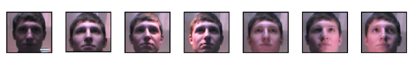
(a) Same pose and identity, different illuminations

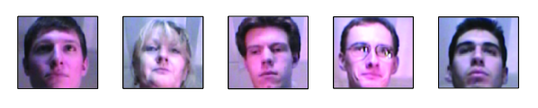
(b) Same illumination, different poses relative to the sources of illumination

Figure 4: (a) Illuminations 1–7 from the Cambridge face motion database. (b) Five different individuals in the illumination setting number 6. In spite of the same spatial arrangement of light sources, their effect on the appearance of faces changes significantly due to variations in people’s heights and the ad lib chosen position relative to the camera.

3.1.2 Amsterdam Library of Object Images

The Amsterdam Library of Object Images is a collection of images of 1000 small objects [22]. Examples of two objects are shown in Figure 5. The data set comprises three main subsets: (i) “Illumination Direction Collection”, (ii) “Illumination Colour Collection” and (iii) “Object View Collection”. In the “Illumination Direction Collection” the camera viewpoint relative to each object was kept constant, while illumination direction was varied. Similarly in the “Illumination Colour Collection”, images corresponding to different voltages of a variable voltage halogen illumination source were acquired from a fixed viewpoint. Finally, “Object View Collection” contains view of objects under a constant illumination but variable pose. These were acquired using 5^∘ increments of the object’s rotation around an axis parallel to the image plane. This collection was used in the evaluation reported here. Figure 5 shows a subset of 10 images (out of the total number of $360/5+1=73$) which illustrate the nature of the data variability. Further detail can be obtained by consulting the original publication [22] and from the web site of the database: www.science.uva.nl/~aloi/.

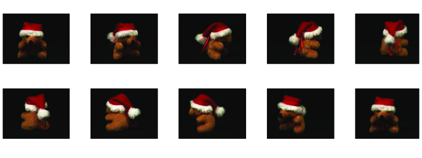
(a) Object 0001 – toy bear

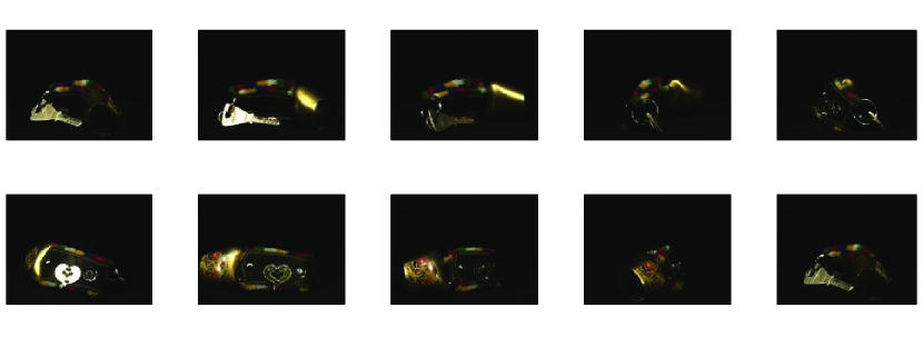
(b) Object 0002 – keys on a chain

Figure 5: Examples of 10 roughly angularly equidistant views (out of 73 available) of two objects from the “Object View Collection” subset of the Amsterdam Library of Object Images [22].

3.2 Evaluation Protocol

In the case of both data sets, evaluation was performed by matching high resolution with low resolution class models. A single class was taken to correspond to a particular person or an object when, respectively, face and object appearance was matched. High resolution linear subspace models were computed using $50\times 50$ pixel face data and $192\times 144$ pixel object images, as described in Section 2. Low resolution subspaces were constructed using downsampled data. Square face images were downsampled to five different scales: $5\times 5$ pixels, $10\times 10$ pixels, $15\times 15$ pixels, $20\times 20$ pixels and $25\times 25$ pixels, as shown in Figure 6 (a). Data from the Amsterdam Library of Object Images was downsampled also to five different scales corresponding to 5%, 10%, 15%, 20% and 25% of its linear scale (e.g. height, while maintaining the original aspect ratio), as shown in Figure 6 (b).

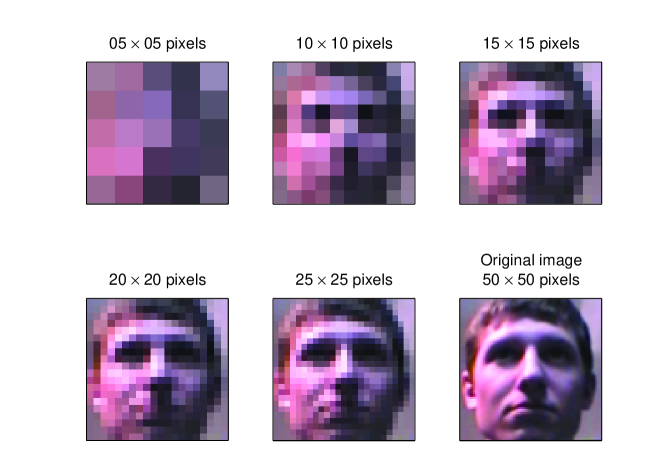
(a) Face scales

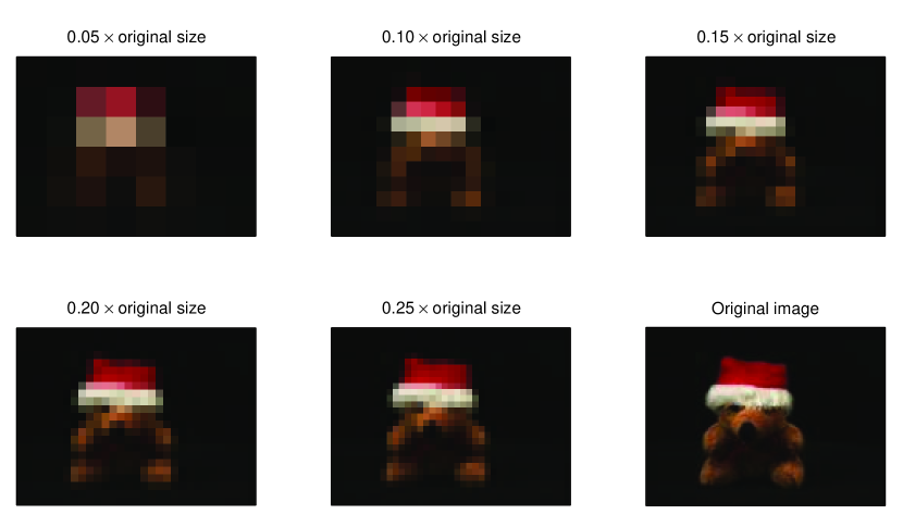
(b) Object scales

Figure 6: Different scales used as low resolution matching input for (a) face and (b) object data. Square face images with the widths of 5 to 25 pixels at 5 pixel increments, were considered. Images from the Amsterdam Library of Object Images were sub-sampled to 5% to 25% of the original size, at 5% increments.

Training was performed by constructing class models with downsampled face images in a single illumination setting in the case of face appearance matching and downsampled object images using half of the available data in the case of object appearance matching. Thus each class represented by a linear subspace corresponds to, respectively, a single person and captures his/her appearance in the training illumination, and a single object using a limited set of views.

In querying an algorithm using a novel subspace, the subspace was classified to the class of the highest similarity. The similarity between two subspaces was expressed by a number in the range $[0,1]$, equal to the correlation of the two highest correlated vectors confined to them, as per Equation (18) in the previous section.

3.3 Results

First, the effects of the method proposed in Section 2.2 on class separation were examined, and compared to that of the naïve method of Section 2.1. This was quantified as follows. For a given pair of training and “query” illumination conditions, the similarity $\rho_{i,j}$ between all image sets $i$ acquired in the training illumination and all sets $j$ acquired in the query illumination was evaluated. Thus, the mean confidences $\overline{e}_{w}$ and $\overline{e}_{b}$ of, respectively, the correct and incorrect matching assignments are given by:

$$\overline{e}_{w} =1-\frac{1}{M}~{}\sum_{i=1}^{M}\rho_{i,i}$$ (28)

$$\overline{e}_{b} =1-\frac{1}{M\times(M-1)}~{}\sum_{i=1}^{M}\sum_{\scriptsize j=1,~{}j\neq i}^{M}\rho_{i,j},$$ (29)

where $M$ is the number of distinct classes. The corresponding separation is then proportional to $\overline{e}_{b}$ and inversely proportional to $\overline{e}_{w}$:

$$\mu=\overline{e}_{b}~{}{\overline{e}_{w}}^{-1}.$$ (30)

The separation was evaluated separately for all training-query illumination pairs in the Cambridge Face Database using the naïve method and compared with that of the proposed solution across different matching scales using the bicubic projection model. A plot of the results is shown in Figure 7 in which for clarity the training-query illumination pairs were ordered in increasing order of improvement for each plot (thus the indices of different abscissae do not necessarily correspond).

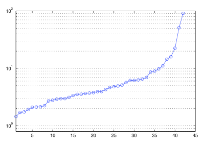
(a) $(5\times 5)\longleftrightarrow(50\times 50)$

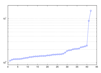
(b) $(10\times 10)\longleftrightarrow(50\times 50)$

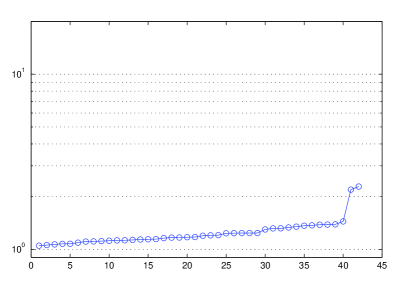
(c) $(15\times 15)\longleftrightarrow(50\times 50)$

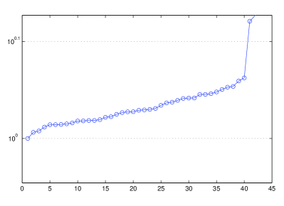
(d) $(20\times 20)\longleftrightarrow(50\times 50)$

Figure 7: The increase in class separation $\mu$ (the ordinate; note that the scale is logarithmic) over different training-query illumination conditions (abscissa), achieved by the proposed method in comparison to the naïve subspace re-projection approach. Note that for clarity the training-query illumination pairs were ordered in increasing order of improvement for each plot; thus, the indices of different abscissae do not necessarily correspond.

Firstly, note that improvement was observed for all illumination combinations at all scales. Unsurprisingly, the most significant increase in class separation ($\approx 8.5$-fold mean increase) was achieved for the most drastic difference in training and query sets, when subspaces embedded in a 25-dimensional image space – representing the appearance variation of images as small as $5\times 5$ pixels, see Figure 6 (a) – was matched against a subspace embedded in the image space of a 100 times greater dimensionality.

It is interesting to note that even at the more favourable scales of the low resolution input, although the mean improvement was less noticeable than at extreme scale discrepancies, the accuracy of matching in certain combinations of illumination settings still greatly benefited from the proposed method. For example, for low resolution subspaces representing appearance in $10\times 10$ pixel images, the mean separation increase of 75.6% was measured; yet, for illuminations “1” and “2” – corresponding to the index 42 on the abscissa in Figure 7 (b) – the improvement was 473.0%. The change effected on the inter-class and intra-class distances is illustrated in Figure 8, which shows a typical similarity matrix produced by the naïve and the proposed matching methods.

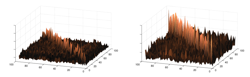
(a) Naïve	(b) Proposed

Figure 8: Typical similarity matrices resulting from the naïve (left) and the proposed (right) matching approaches. Our method produces a dramatic improvement in class separation as witnessed by the increased dominance of the diagonal elements in the aforementioned matrix.

The mean separation increase across different scales for face and object data is shown in, respectively, Figures 9 and 10. These also illustrate the impact that the projection model used has on the quality of matching results, Figures 9 (a) and 10 (a) corresponding to the bilinear projection model, and Figures 9 (b) and 10 (b) to the bicubic. As could be expected from theory, the latter was found to be consistently superior across all scales and for both data sets. In the case of face appearance, the greatest improvement over the naïve re-projection method was observed for the smallest scale of low resolution data – $8.5$-fold separation increase was achieved for $5\times 5$ pixel images, $1.75$-fold for $10\times 10$, $1.25$-fold for $15\times 15$, $1.08$-fold for $20\times 20$ and $1.03$-fold for $25\times 25$. It is interesting to note that the relative performance across different scales of low resolution object data did not follow the same functional form as in the case of face data. A possible reason for this seemingly odd result lies in the presence of confounding background regions (unlike in the face data set, which was automatically cropped to include foreground information only). Not only does the background typically occupy a significant area of object images, it is also of variable shape across different views of the same object, as well as across different objects. It is likely that the interaction of this confounding factor with the downsampling scale is the cause of the less predictable nature of the plots in Figure 10.

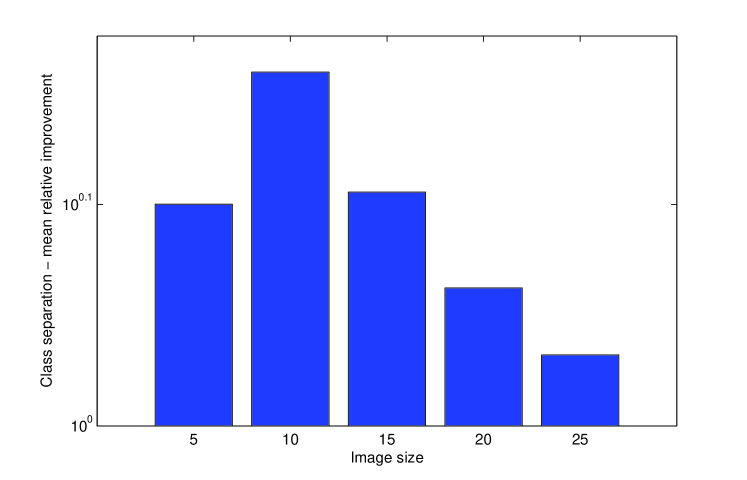
(a) Faces – bilinear projection model

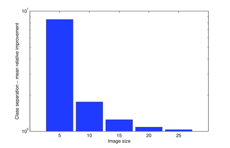
(b) Faces – bicubic projection model

Figure 9: Mean class separation increase achieved, as a function of size of the low-scale images. Shown is the ratio of class separation when subspaces are matched using the proposed method and the naïve re-projection method described in Section 2.1. The rate of improvement decay is incrementally exponential, reaching 1 (no improvement) when $d_{l}=d_{h}$.

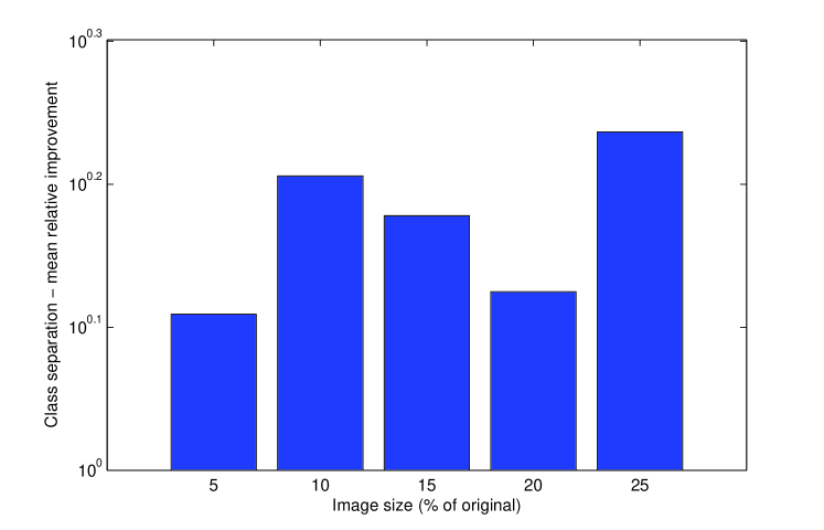
(a) Objects – bilinear projection model

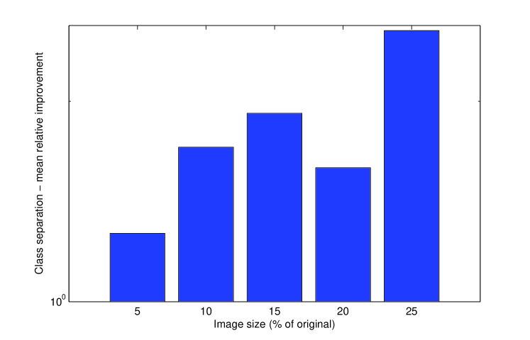
(b) Objects – bicubic projection model

Figure 10: Mean class separation increase achieved, as a function of size of the low-scale images. Shown is the ratio of class separation when subspaces are matched using the proposed method and the naïve re-projection method. Unlike in the plots obtained from face matching experiments in Figure 9, the nature of variation across different scales here appears less regular. It is likely that the reason lies in the large (and variable in shape) area of the background present in the object images.

The inferred most similar modes of variation contained within two subspaces representing face appearance variation of the same person in different illumination conditions and at different training scales for the bilinear and bicubic models respectively are shown in Figures 11 and 12. In both cases, as the scale of low-resolution images is reduced, the naïve algorithm of Section 2.1 finds progressively worse matching modes with significant visual degradation in the mode corresponding to the low-resolution subspace. In contrast, the proposed algorithm correctly reconstructs meaningful high-resolution appearance even in the case of extremely low resolution images ($5\times 5$ pixels).

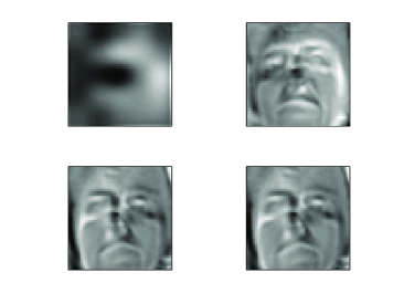
(a) $(5\times 5)\longleftrightarrow(50\times 50)$

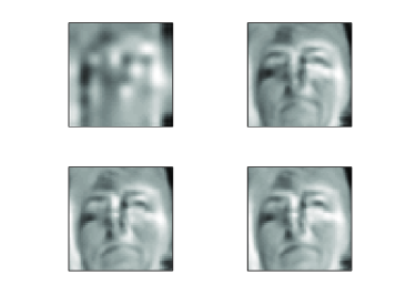
(b) $(10\times 10)\longleftrightarrow(50\times 50)$

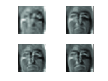
(c) $(15\times 15)\longleftrightarrow(50\times 50)$

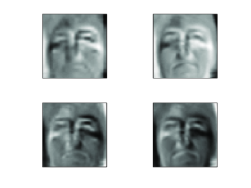
(d) $(20\times 20)\longleftrightarrow(50\times 50)$

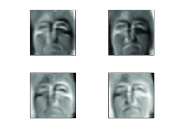
(e) $(25\times 25)\longleftrightarrow(50\times 50)$

Figure 11: Bicubic projection model – the inferred most similar modes of variation contained within two subspaces representing face appearance variation of the same person in different illumination conditions and at different training scales. In each subfigure, which corresponds to a different training-query scale discrepancy, the top pair of images represents appearance extracted by the naïve algorithm of Section 2.1 (as the left-singular and right-singular vectors of ${\mathbf{B}_{Y}}^{T}~{}\mathbf{B}^{*}_{X}$); the bottom pair is extracted by the proposed method (as the left-singular and right-singular vectors of ${\mathbf{B}_{Y}}^{T}~{}\mathbf{B}_{Xc}$).

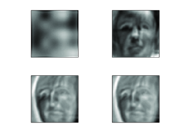
(a) $(5\times 5)\longleftrightarrow(50\times 50)$

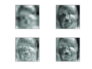
(b) $(10\times 10)\longleftrightarrow(50\times 50)$

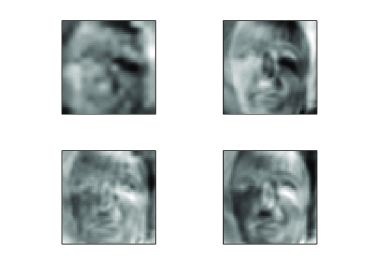
(c) $(15\times 15)\longleftrightarrow(50\times 50)$

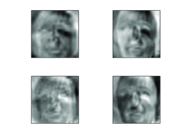
(d) $(20\times 20)\longleftrightarrow(50\times 50)$

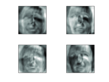
(e) $(25\times 25)\longleftrightarrow(50\times 50)$

Figure 12: Bilinear projection model – the inferred most similar modes of variation contained within two subspaces representing face appearance variation of the same person in different illumination conditions and at different training scales. In each subfigure, which corresponds to a different training-query scale discrepancy, the top pair of images represents appearance extracted by the naïve algorithm of Section 2.1 (as the left-singular and right-singular vectors of ${\mathbf{B}_{Y}}^{T}~{}\mathbf{B}^{*}_{X}$); the bottom pair is extracted by the proposed method (as the left-singular and right-singular vectors of ${\mathbf{B}_{Y}}^{T}~{}\mathbf{B}_{Xc}$).

Lastly, we examined the behaviour of the proposed method in the presence of data corruption by noise. Specifically, we repeated the previously described experiments for the bilinear projection model with the difference that following the downsampling of high resolution images we added pixel-wise Gaussian noise to the resulting low resolution images before creating the corresponding low-dimensional subspaces. Since pixel-wise characteristics of noise were the same across all pixels in a specific experiment, this noise is isotropic in the low-dimensional image space. The sensitivity of the proposed method was evaluated by varying the magnitude of noise added in this manner. In particular, we started by adding noise with pixel-wise standard deviation of 1 (i.e. image space root mean square equal to $\sqrt{D_{l}}$) , or approximately 0.4% of the entire greyscale spanning the range from 0 to 255, and progressively increased up to 30 (i.e. image space root mean square equal to $30\sqrt{D_{l}}$), or approximately 12% of the possible pixel value range which corresponds to the average signal-to-noise ratio of only $1.7$. The results are summarized in the plot in Figure 13 which shows the change in class separation for different levels of additive noise. Note that for the sake of easier visualization in a single plot, the change is shown relative to the separation attained using un-corrupted images, discussed previously and plotted in Figure 9(a). It is remarkable to observe that even in the most challenging experiment, when the magnitude of added noise is extreme, the performance of the proposed method is hardly affected at all. In all cases, including that when matching is performed using low-dimensional subspaces with the greatest downsampling factor, the average class separation is not decreased more than 1.5%. For pixel-wise noise magnitudes of up to 20 greyscale levels, the deterioration is consistently lower than 0.5%, and even for the pixel-wise noise magnitude of 30 greyscale levels the separation decrease of more than 1% is observed in only two instances (for low-dimensional spaces corresponding to images downsampled to $10\times 10$ and $15\times 15$ pixels). Note that this means that even when the proposed method performs matching in the presence of extreme noise, its performance exceeds that of the naïve approach applied to un-corrupted data.

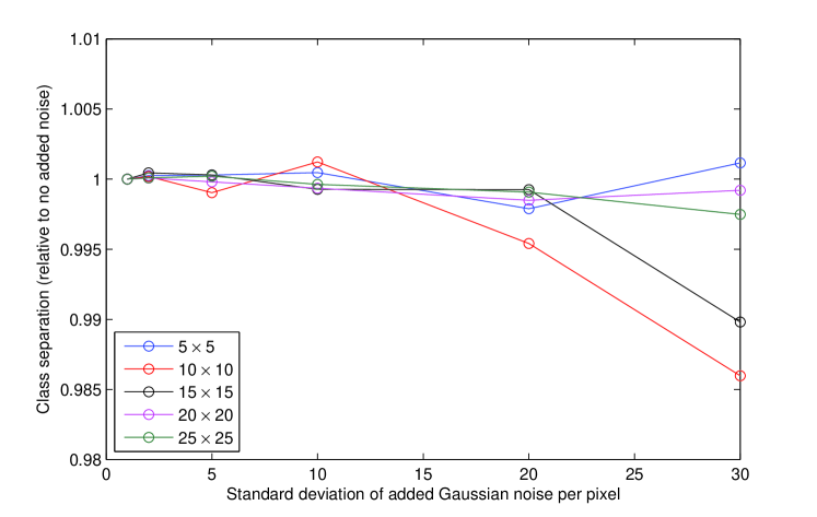
Figure 13: The effects of additive zero-mean Gaussian noise, isotropic in the image space, applied to low resolution images before the construction of the corresponding subspaces. Shown is the change in the observed class separation which is for the sake of visualization clarity measured relative to the separation achieved using the original, un-corrupted images; see Figure 9(a). The results are for the bilinear projection model. Notice the remarkable robustness of the proposed model: even for noise with the pixel-wise standard deviation of 30 greyscale levels (approximately 12% of the entire greyscale intensity range), which corresponds to the average signal-to-noise ratio of 1.7, class separation is decreased by less than 1.5%. Note that this means that even when the proposed method performs matching in the presence of extreme noise, its performance exceeds that of the naïve approach applied to un-corrupted data.

4 Conclusion

In this paper a method for matching linear subspaces which represent appearance variations in images of different scales was described. The approach consists of an initial re-projection of the subspace in the low-dimensional image space to the high-dimensional one, and subsequent refinement of the re-projection through a constrained rotation. Using facial and object appearance images and the corresponding two large data sets, it was shown that the proposed algorithm successfully reconstructs the personal subspace in the high-dimensional image space even for low-dimensional input corresponding to images as small as $5\times 5$ pixels, improving average class separation by an order of magnitude. Our immediate future work will be in the direction of integrating the proposed method with the discriminative framework recently described in [23].

References

- [1] V. Ferrari, T. Tuytelaars, , and L. Van Gool. Retrieving objects from videos based on affine regions. In Proc. European Signal Processing Conference (EUSIPCO), pages 128–131, 2004.
- [2] M. Everingham, A. Zisserman, C. Williams, C. Van Gool, et al. The 2005 PASCAL visual object classes challenge. In Selected Proc. First PASCAL Challenges Workshop, 2006.
- [3] Y. Su, S. Shan, X. Chen, and W. Gao. Hierarchical ensemble of global and local classifiers for face recognition. IEEE Transactions on Image Processing (TIP), 18(8):1885–1896, 2009.
- [4] R. Pradhan, Z. G. Bhutia, M. Nasipuri, and M. P. Pradhan. Gradient and principal component analysis based texture recognition system: A comparative study. Fifth International Conference on Information Technology: New Generations, pages 1222–1223, 2009.
- [5] R. Hartley and A. Zisserman. Multiple view geometry in computer vision. 2nd edition, 2004.
- [6] P. Chen and D. Suter. An analysis of linear subspace approaches for computer vision and pattern recognition. International Journal of Computer Vision (IJCV), 68(1):83–106, 2006.
- [7] M. Bethge. Factorial coding of natural images: how effective are linear models in removing higher-order dependencies? Journal of the Optical Society of America (JOSA A), 23(6):1253–1268, 2006.
- [8] P. N. Belhumeur and D. J. Kriegman. What is the set of images of an object under all possible illumination conditions? International Journal of Computer Vision (IJCV), 28(3):245–260, 1998.
- [9] A. S. Georghiades, P. N. Belhumeur, and D. J. Kriegman. From few to many: Illumination cone models for face recognition under variable lighting and pose. IEEE Transactions on Pattern Analysis and Machine Intelligence (TPAMI), 23(6):643–660, 2001.
- [10] R. Basri and D. W. Jacobs. Lambertian reflectance and linear subspaces. IEEE Transactions on Pattern Analysis and Machine Intelligence (TPAMI), 25(2):218–233, 2003.
- [11] K. Lee, M. Ho, J. Yang, and D. Kriegman. Acquiring linear subspaces for face recognition under variable lighting. IEEE Transactions on Pattern Analysis and Machine Intelligence (TPAMI), 27(5):684–698, 2005.
- [12] S. Zhou, G. Aggarwal, R. Chellappa, and D. Jacobs. Appearance characterization of linear lambertian objects, generalized photometric stereo, and illumination-invariant face recognition. IEEE Transactions on Pattern Analysis and Machine Intelligence (TPAMI), 29(2):230–245, 2007.
- [13] D. Skočaj and A. Leonardis. Weighted and robust incremental method for subspace learning. Image and Vision Computing (IVC), pages 27–38, 2008.
- [14] M. Song and H. Wang. Highly efficient incremental estimation of Gaussian mixture models for online data stream clustering. In Proc. SPIE Conference on Intelligent Computing: Theory And Applications, 2005.
- [15] O. Arandjelović and R. Cipolla. Incremental learning of temporally-coherent Gaussian mixture models. In Proc. British Machine Vision Conference (BMVC), 2:759–768, 2005.
- [16] J. J. Verbeek, N. Vlassis, and B. Kröse. Efficient greedy learning of Gaussian mixture models. Neural Computation, 5(2):469–485, 2003.
- [17] P. Hall, D. Marshall, and R. Martin. Merging and splitting eigenspace models. IEEE Transactions on Pattern Analysis and Machine Intelligence (TPAMI), 22(9):1042–1048, 2000.
- [18] R. Gross, J. Yang, and A. Waibel. Growing Gaussian mixture models for pose invariant face recognition. In Proc. IAPR International Conference on Pattern Recognition (ICPR), 1:1088–1091, 2000.
- [19] A.S. Householder. Unitary triangularization of a nonsymmetric matrix. Journal of the ACM, 5(4):339–342, 1958.
- [20] O. Arandjelović. Recognition from appearance subspaces across image sets of variable scale. In Proc. British Machine Vision Conference (BMVC), 2010. DOI: 10.5244/C.24.79.
- [21] O. Arandjelović. Computationally efficient application of the generic shape-illumination invariant to face recognition from video. Pattern Recognition (PR), 45(1):92–103, 2012.
- [22] J. M. Geusebroek, G. J. Burghouts, and A. W. M. Smeulders. The Amsterdam library of object images. International Journal of Computer Vision (IJCV), 61(1):103–112, 2005.
- [23] O. Arandjelović. Discriminative extended canonical correlation analysis for pattern set matching. Machine Learning (ML), 2013. DOI: 10.1007/s10994-013-5380-5.