The Galerkin Finite Element Method for A Multi-term Time-Fractional Diffusion equation

Abstract.

We consider the initial/boundary value problem for a diffusion equation involving multiple time-fractional derivatives on a bounded convex polyhedral domain. We analyze a space semidiscrete scheme based on the standard Galerkin finite element method using continuous piecewise linear functions. Nearly optimal error estimates for both cases of initial data and inhomogeneous term are derived, which cover both smooth and nonsmooth data. Further we develop a fully discrete scheme based on a finite difference discretization of the time-fractional derivatives, and discuss its stability and error estimate. Extensive numerical experiments for one and two-dimension problems confirm the convergence rates of the theoretical results.
Keywords: multi-term time-fractional diffusion equation, finite element method, error estimate, semidiscrete scheme, Caputo derivative

1. introduction

We consider the following initial/boundary value problem for a multi-term time fractional diffusion equation in $u(x,t)$:

$$P(\partial_{t})u-\Delta u =f, \quad\text{in }\Omega \quad T\geq t>0,$$

(1.1) $$u =0, \quad\text{on}\ \partial\Omega \quad T\geq t>0,$$

$$u(0) =v, \quad\text{in }\Omega,$$

where $\Omega$ denotes a bounded convex polygonal domain in $\mathbb{R}^{d}\,(d=1,2,3)$ with a boundary $\partial\Omega$, $f$ is the source term, and the initial data $v$ is a given function on $\Omega$ and $T>0$ is a fixed value. Here the differential operator $P(\partial_{t})$ is defined by

$$P(\partial_{t})=\partial_{t}^{\alpha}+\sum_{i=1}^{m}b_{i}\partial_{t}^{\alpha_{i}},$$

where $0<\alpha_{m}\leq...\leq\alpha_{1}<\alpha<1$ are the orders of the fractional derivatives, $b_{i}>0$, $i=1,2,...,m$, with the left-sided Caputo fractional derivative $\partial_{t}^{\beta}u$ being defined by (cf. [17, pp. 91])

(1.2) $$\partial_{t}^{\beta}u(t)=\frac{1}{\Gamma(1-\beta)}\int_{0}^{t}(t-\tau)^{-\beta}\frac{d}{d\tau}u(\tau)d\tau,$$

where $\Gamma(\cdot)$ denotes the Gamma function.

In the case of $m=0$, the model (1) reduces to its single-term counterpart

(1.3) $$\partial_{t}^{\alpha}u-\Delta u=f\quad\mbox{ in }\Omega\times(0,T].$$

This model has been studied extensively from different aspects due to its extraordinary capability of modeling anomalous diffusion phenomena in highly heterogeneous aquifers and complex viscoelastic materials [1, 29]. It is the fractional analogue of the classical diffusion equation: with $\alpha=1$, it recovers the latter, and thus inherits some of its analytical properties. However, it differs considerably from the latter in the sense that, due to the presence of the nonlocal fractional derivative term, it has limited smoothing property in space and slow asymptotic decay in time [30], which in turn also impacts related numerical analysis [12] and inverse problems [14, 30].

The model (1) was developed to improve the modeling accuracy of the single-term model (1.3) for describing anomalous diffusion. For example, in [31], a two-term fractional-order diffusion model was proposed for the total concentration in solute transport, in order to distinguish explicitly the mobile and immobile status of the solute using fractional dynamics. The kinetic equation with two fractional derivatives of different orders appears also quite naturally when describing subdiffusive motion in velocity fields [26]; see also [16] for discussions on the model for wave-type phenomena.

There are very few mathematical studies on the model (1). Luchko [23] established a maximum principle for problem (1), and constructed a generalized solution for the case $f\equiv 0$ using the multinomial Mittag-Leffler function. Jiang et al [9] derived analytical solutions for the diffusion equation with fractional derivatives in both time and space. Li and Yamamoto [20] established existence, uniqueness, and the Hölder regularity of the solution using a fixed point argument for problem (1) with variable coefficients $\{b_{i}\}$. Very recently, Li et al [19] showed the uniqueness and continuous dependence of the solution on the initial value $v$ and the source term $f$, by exploiting refined properties of the multinomial Mittag-Leffler function.

The applications of the model (1) motivate the design and analysis of numerical schemes that have optimal (with respect to data regularity) convergence rates. Such schemes are especially valuable for problems where the solution has low regularity. The case $m=0$, i.e., the single-term model (1.3), has been extensively studied, and stability and error estimates were provided; see [21, 35] for the finite difference method, [18, 34] for the spectral method, [25, 27, 28, 12, 11, 10] for the finite element method, and [3, 7] for meshfree methods based on radial basis functions, to name a few. In particular, in [10, 11, 12], the authors established almost optimal error estimates with respect to the regularity of the initial data $v$ and the right hand side $f$ for a semidiscrete Galerkin scheme. These studies include the interesting case of very weak data, i.e., $v\in\dot{H}^{q}(\Omega)$ and $f\in L^{\infty}(0,T;\dot{H}^{q}(\Omega))$ for $-1<q\leq 0$.

Numerical methods for the general multi-term case for an ordinary differential equation were considered in [15, 6]. In [36], a scheme based on the finite element method in space and a specialized finite difference method in time was proposed for (1), and error estimates were derived. We also refer to [22] for a numerical scheme based on a fractional predictor-corrector method for the multi-term time fractional wave-diffusion equation. The error analysis in these works is done under the assumption that the solution is sufficiently smooth and therefore it excludes the case of low regularity solutions. This is the main goal of the present study. However, the derivation of optimal with respect to the regularity error estimates requires additional analysis of the properties of problem (1), e.g., stability, asymptotic behavior for $t\to 0^{+}$. Relevant results of this type have recently been obtained in [19], which, however, are not enough for the analysis of the semidiscrete Galerkin scheme, and hence in Section 2, we make the necessary extensions.

Now we describe the semidiscrete Galerkin scheme. Let ${\{\mathcal{T}_{h}\}}_{0<h<1}$ be a family of shape regular and quasi-uniform partitions of the domain $\Omega$ into $d$-simplexes, called finite elements, with a maximum diameter $h$. The approximate solution $u_{h}$ is sought in the finite element space $X_{h}$ of continuous piecewise linear functions over the triangulation $\mathcal{T}_{h}$

$$X_{h}=\left\{\chi\in H^{1}_{0}(\Omega):\ \chi~{}~{}\mbox{is a linear function over}~{}~{}\tau,\,\,\,\,\forall\tau\in\mathcal{T}_{h}\right\}.$$

The semidiscrete Galerkin FEM for problem (1) is: find $u_{h}(t)\in X_{h}$ such that

(1.4) $${(P(\partial_{t})u_{h},\chi)}+a(u_{h},\chi)={(f,\chi)},\quad\forall\chi\in X_{h},\ T\geq t>0,\quad u_{h}(0)=v_{h},$$

where $a(u,w)=(\nabla u,\nabla w)~{}~{}\text{for}\ u,\,w\in H_{0}^{1}(\Omega)$, and $v_{h}\in X_{h}$ is an approximation of the initial data $v$. The choice of $v_{h}$ will depend on the smoothness of the initial data $v$. We shall study the convergence of the semidiscrete scheme (1.4) for the case of initial data $v\in\dot{H}^{q}(\Omega)$, $-1<q\leq 2$, and right hand side $f\in L^{\infty}(0,T;\dot{H}^{q}(\Omega))$, $-1<q<1$. The case of nonsmooth data, i.e., $-1<q\leq 0$, is very common in inverse problems and optimal control [14, 30]; see also [33, 13, 4, 5] for the parabolic counterpart.

The goal of this work is to develop a numerical scheme based on the finite element approximation for the model (1), and provide a complete error analysis. We derive error estimates optimal with respect to the data regularity for the semidiscrete scheme, and a convergence rate $O(h^{2}+\tau^{2-\alpha})$ for the fully discrete scheme in case of a smooth solution. Specifically, our essential contributions are as follows. First, we obtain an improved regularity result for the inhomogeneous problem, by allowing less regular source term, cf. Theorem 2.3. This is achieved by first establishing a new result, i.e., the complete monotonicity of the multinomial Mittag-Leffler function, cf. Lemma 2.4. Second, we derive nearly optimal error estimates for a semidiscrete Galerkin scheme for both homogeneous and inhomogeneous problems, cf. Theorems 3.1-3.4, which cover both smooth and nonsmooth data. Third, we develop a fully discrete scheme based on a finite difference method in time, and establish its stability and error estimates, cf. Theorem 4.1. We note that the derived error estimate for the fully discrete scheme holds only for smooth solutions.

The rest of the paper is organized as follows. In Section 2, we recall the solution theory for the model (1) for both homogeneous and inhomogeneous problems, using properties of the multinomial Mittag-Leffler function. The readers not interested in the analysis may proceed directly to Section 3. Almost optimal error estimates for their Galerkin finite element approximations are given in Section 3. Then a fully discrete scheme based on a finite difference approximation of the Caputo fractional derivatives is given in Section 4, and an error analysis is also provided. Finally, extensive numerical experiments are presented to illustrate the accuracy and efficiency of the Galerkin scheme, and to verify the convergence theory. Throughout, we denote by $C$ a generic constant, which may differ at different occurrences, but always independent of the mesh size $h$ and time step size $\tau$.

2. Solution theory

In this part, we recall the solution theory for problem (1). We shall describe the solution representation using the multinomial Mittag-Leffler function, and derive optimal solution regularity for the homogeneous and inhomogeneous problems.

2.1. Multinomial Mittag-leffler function

First we recall the multinomial Mittag-Leffler function, introduced in [8]. For $0<\beta<2$, $0<\beta_{i}<1$ and $z_{i}\in\mathbb{C}$, $i=1,...,m$, the multinomial Mittag-Leffler function $E_{(\beta_{1},...,\beta_{m}),\beta}(z_{1},...,z_{m})$ is defined by

$$E_{(\beta_{1},...,\beta_{m}),\beta}(z_{1},...,z_{m})=\sum_{k=0}^{\infty}\sum_{\begin{subarray}{c}l_{1}+...+l_{m}=k\\ l_{1}\geq 0,...,l_{m}\geq 0\end{subarray}}(k;l_{1},...,l_{m})\frac{\prod_{i=1}^{m}z_{i}^{l_{i}}}{\Gamma(\beta+\Sigma_{i=1}^{m}\beta_{i}l_{i})},$$

where the notation $(k;l_{1},...,l_{m})$ denotes the multinomial coefficient, i.e.,

$$(k;l_{1},...,l_{m})=\frac{k!}{l_{1}!...l_{m}!}\quad\mbox{with }k=\sum_{i=1}^{m}l_{i}.$$

It generalizes the exponential function $e^{z}$: with $m=1$ and $\beta=\beta_{1}=1$, it reproduces the exponential function $e^{z}$. It appears in the solution representation of problem (1), cf. (2.4) below. We shall need the following two important lemmas on the function $E_{(\beta_{1},...,\beta_{m}),\beta}(z_{1},...,z_{m})$, recently obtained in [19, Section 2.1].

Lemma 2.1.

Let $0<\beta<2$, $0<\beta_{i}<1$, $\beta_{1}>\max\{\beta_{2},...,\beta_{m}\}$ and $\frac{\beta_{1}\pi}{2}<\mu<\beta_{1}\pi$. Assume that there is $K>0$ such that $-K\leq z_{i}<0$, $i=2,...,m$. Then there exists a constant $C=C(\beta_{1},...,\beta_{m},\beta,K,\mu)>0$ such that

$$E_{(\beta_{1},...,\beta_{m}),\beta}(z_{1},...,z_{m})\leq\frac{C}{1+|z_{1}|},\quad\quad\quad\mu\leq|\mathrm{arg}(z_{1})|\leq\pi.$$

Lemma 2.2.

Let $0<\beta<2$, $0<\beta_{i}<1$ and $z_{i}\in\mathbb{C}$, $i=1,...,m$. Then we have

$$\frac{1}{\Gamma(\beta_{0})}+\sum_{i=1}^{m}z_{i}E_{(\beta_{1},...,\beta_{m}),{\beta_{0}+\beta_{i}}}(z_{1},...,z_{m})=E_{(\beta_{1},...,\beta_{m}),\beta_{0}}(z_{1},...,z_{m}).$$

2.2. Solution Representation

For $s\geq-1$, we denote by $\dot{H}^{s}(\Omega)\subset H^{-1}(\Omega)$ the Hilbert space induced by the norm:

$$\|v\|_{\dot{H}^{s}(\Omega)}^{2}=\sum_{j=1}^{\infty}\lambda_{j}^{s}\langle v,\varphi_{j}\rangle^{2}$$

with $\{\lambda_{j}\}_{j=1}^{\infty}$ and $\{\varphi_{j}\}_{j=1}^{\infty}$ being respectively the eigenvalues and the $L^{2}(\Omega)$-orthonormal eigenfunctions of the Laplace operator $-\Delta$ on the domain $\Omega$ with a homogeneous Dirichlet boundary condition. Then $\{\varphi_{j}\}_{j=1}^{\infty}$ and $\{\lambda_{j}^{1/2}\varphi_{j}\}_{j=1}^{\infty}$, form an orthonormal basis in $L^{2}(\Omega)$ and $H^{-1}(\Omega)$, respectively. Further, $\|v\|_{\dot{H}^{0}(\Omega)}=\|v\|_{L^{2}(\Omega)}=(v,v)^{1/2}$ is the norm in $L^{2}(\Omega)$ and $\|v\|_{\dot{H}^{-1}(\Omega)}=\|v\|_{H^{-1}(\Omega)}$ is the norm in $H^{-1}(\Omega)$. It is easy to verify that $\|v\|_{\dot{H}^{1}(\Omega)}=\|\nabla v\|_{L^{2}(\Omega)}$ is also the norm in $H_{0}^{1}(\Omega)$ and $\|v\|_{\dot{H}^{2}(\Omega)}=\|\Delta v\|_{L^{2}(\Omega)}$ is equivalent to the norm in $H^{2}(\Omega)\cap H^{1}_{0}(\Omega)$ [32, Lemma 3.1]. Note that $\dot{H}^{s}(\Omega)$, $s\geq-1$ form a Hilbert scale of interpolation spaces. Hence, we denote $\|\cdot\|_{H^{s}(\Omega)}$ to be the norm on the interpolation scale between $H^{1}_{0}(\Omega)$ and $L^{2}(\Omega)$ for $s\in[0,1]$ and $\|\cdot\|_{H^{s}(\Omega)}$ to be the norm on the interpolation scale between $L^{2}(\Omega)$ and $H^{-1}(\Omega)$ for $s\in[-1,0]$. Then, $\|\cdot\|_{H^{s}(\Omega)}$ and $\|\cdot\|_{\dot{H}^{s}(\Omega)}$ are equivalent for $s\in[-1,1]$. Further, for a Banach space $B$, we define the space

$$L^{r}(0,T;B)=\{u(t)\in B\mbox{ for a.e. }t\in(0,T)\mbox{ and }\|u\|_{L^{r}(0,T;B)}<\infty\},$$

for any $r\geq 1$, and the norm $\|\cdot\|_{L^{r}(0,T;B)}$ is defined by

$$\|u\|_{L^{r}(0,T;B)}=\left\{\begin{aligned} \left(\int_{0}^{T}\|u(t)\|_{B}^{r}dt\right)^{1/r},&\quad r\in[1,\infty),\\ \displaystyle{\mathrm{esssup}_{t\in(0,T)}}\|u(t)\|_{B},&\quad r=\infty.\end{aligned}\right.$$

Upon denoting ${\vec{\alpha}}=(\alpha,\alpha-\alpha_{1},...,\alpha-\alpha_{m})$, we introduce the following solution operator

(2.1) $$E(t)v=\sum_{j=1}^{\infty}\left(1-\lambda_{j}t^{\alpha}E_{{\vec{\alpha}},1+\alpha}(-\lambda_{j}t^{\alpha},-b_{1}t^{\alpha-\alpha_{1}},...,-b_{m}t^{\alpha-\alpha_{m}})\right)(v,\varphi_{j})\varphi_{j}.$$

This operator is motivated by a separation of variable [24, 23]. Then for problem (1) with a homogeneous right hand side, i.e., $f\equiv 0$, we have $u(x,t)=E(t)v$. However, the representation (2.1) is not always very convenient for analyzing its smoothing property. We derive an alternative representation of the solution operator $E$ using Lemma 2.2:

(2.2) $$\begin{split}E(t)v=&\sum_{j=1}^{\infty}E_{{\vec{\alpha}},1}(-\lambda_{j}t^{\alpha},-b_{1}t^{\alpha-\alpha_{1}},...,-b_{m}t^{\alpha-\alpha_{m}})(v,\varphi_{j})\varphi_{j}\\ &\ \ +\sum_{i=1}^{m}b_{i}t^{\alpha-\alpha_{i}}\sum_{j=1}^{\infty}E_{{\vec{\alpha}},1+\alpha-\alpha_{i}}(-\lambda_{j}t^{\alpha},-b_{1}t^{\alpha-\alpha_{1}},...,-b_{m}t^{\alpha-\alpha_{m}})(v,\varphi_{j})\varphi_{j}.\end{split}$$

Besides, we define the following operator $\bar{E}$ for $\chi\in L^{2}(\Omega)$ by

(2.3) $$\bar{E}(t)\chi=\sum_{j=1}^{\infty}t^{\alpha-1}E_{{\vec{\alpha}},\alpha}(-\lambda_{j}t^{\alpha},-b_{1}t^{\alpha-\alpha_{1}},...,-b_{m}t^{\alpha-\alpha_{m}})(\chi,\varphi_{j})\varphi_{j}.$$

The operators $E(t)$ and ${\bar{E}}(t)$ can be used to represent the solution $u$ of (1) as:

(2.4) $$u(t)=E(t)v+\int_{0}^{t}{\bar{E}}(t-s)f(s)ds.$$

The operator $\bar{E}$ has the following smoothing property.

Lemma 2.3.

For any $t>0$ and $\chi\in\dot{H}^{q}(\Omega)$, $q\in(-1,2]$, there holds for $0\leq p-q\leq 2$

$$\|\bar{E}(t)\chi\|_{\dot{H}^{p}(\Omega)}\leq Ct^{-1+\alpha(1+(q-p)/2)}\|\chi\|_{\dot{H}^{q}(\Omega)}.$$

Proof.

The definition of the operator $\bar{E}$ in (2.3) and Lemma 2.1 yield

$$\begin{split}\|\bar{E}(t)\chi\|_{\dot{H}^{p}(\Omega)}^{2}&=t^{-2+(2+q-p)\alpha}\sum_{j=1}^{\infty}(\lambda_{j}t^{\alpha})^{p-q}|E_{{\vec{\alpha}},\alpha}(-\lambda_{j}t^{\alpha},-b_{1}t^{\alpha-\alpha_{1}},...,-b_{m}t^{\alpha-\alpha_{m}})|^{2}\lambda_{j}^{q}|(\chi,\varphi_{j})|^{2}\\ &\leq Ct^{-2+(2+q-p)\alpha}\sum_{j=1}^{\infty}\frac{(\lambda_{j}t^{\alpha})^{p-q}}{(1+\lambda_{j}t^{\alpha})^{2}}\lambda_{j}^{q}|(\chi,\varphi_{j})|^{2}\\ &\leq Ct^{-2+(2+q-p)\alpha}\sum_{j=1}^{\infty}\lambda_{j}^{q}|(\chi,\varphi_{j})|^{2}\leq Ct^{-2+(2+q-p)\alpha}\|\chi\|_{\dot{H}^{q}(\Omega)},\end{split}$$

where the last line follows by the inequality $\sup_{j\in\mathbb{N}}\frac{(\lambda_{j}t^{\alpha})^{p-q}}{(1+\lambda_{j}t^{\alpha})^{2}}\leq C$, for $0\leq p-q\leq 2$. ∎

2.3. Solution regularity

First we recall known regularity results. In [20], Li and Yamamoto showed that in the case of variable coefficients $\{b_{i}(x)\}$, there exists a unique mild solution $u\in C((0,T];\dot{H}^{\gamma}(\Omega))\cap C([0,T];L^{2}(\Omega))$ and $u\in C([0,T];\dot{H}^{\gamma}(\Omega))\cap L^{\infty}(0,T;\dot{H}^{2}(\Omega))$ when $v\in L^{2}(\Omega)$, $f=0$ and $v=0$, $f\in L^{\infty}(0,T];L^{2}(\Omega))$, respectively, with $\gamma\in[0,1)$. These results were recently refined in [19] for the case of constant coefficients, i.e., problem (1). In particular, it was shown that for $v\in\dot{H}^{q}(\Omega)$, $0\leq q\leq 1$, and $f=0$, $u\in L^{1/(1-q/2)}(0,T;H^{2}(\Omega)\cap H_{0}^{1}(\Omega))$; and for $v=0$ and $f\in L^{r}(0,T;\dot{H}^{q}(\Omega))$, $0\leq q\leq 2$, $r\geq 1$, $u\in L^{r}(0,T;\dot{H}^{q+2-\gamma}(\Omega))$ for some $\gamma\in(0,1]$. Here we follow the approach in [19], and extend these results to a slightly more general setting of $v\in\dot{H}^{q}(\Omega)$, $-1<q\leq 2$, and $f\in L^{2}(0,T;\dot{H}^{q}(\Omega))$, $-1<q\leq 1$. The nonsmooth case, i.e., $-1<q\leq 0$, arises commonly in related inverse problems and optimal control problems.

We shall derive the solution regularity to the homogeneous problem, i.e., $f\equiv 0$, and the inhomogeneous problem, i.e., $v\equiv 0$, separately. These results will be essential for the error analysis of the space semidiscrete Galerkin scheme in Section 3. First we consider the homogeneous problem with initial data $v\in\dot{H}^{q}(\Omega)$, $-1<q\leq 2$.

Theorem 2.1.

Let $u(t)=E(t)v$ be the solution to problem (1) with $f\equiv 0$ and $v\in\dot{H}^{q}(\Omega)$, $q\in(-1,2]$. Then there holds

$$\|P(\partial_{t})^{\ell}u(t)\|_{\dot{H}^{p}(\Omega)}\leq Ct^{-\alpha(\ell+(p-q)/2)}\|v\|_{\dot{H}^{q}(\Omega)},\quad t>0,$$

where for $\ell=0$, $0\leq p-q\leq 2$ and for $\ell=1$, $-2\leq p-q\leq 0$.

Proof.

We show that (2.2) represents indeed the weak solution to problem (1) with $f\equiv 0$ and further it satisfies the desired estimate. We first discuss the case $\ell=0$. By Lemma 2.1 and (2.2) we have for $0\leq p-q\leq 2$

$$\begin{split}\|E(t)v\|_{\dot{H}^{p}(\Omega)}^{2}&=\displaystyle\sum_{j=1}^{\infty}\lambda_{j}^{p}\Big{(}E_{{\vec{\alpha}},1}(-\lambda_{j}t^{\alpha},-b_{1}t^{\alpha-\alpha_{1}},...,-b_{m}t^{\alpha-\alpha_{m}})\Big{.}\\ &\Big{.}\quad\quad+\sum_{i=1}^{m}b_{i}t^{\alpha-\alpha_{i}}E_{{\vec{\alpha}},1+\alpha-\alpha_{i}}(-\lambda_{j}t^{\alpha},-b_{1}t^{\alpha-\alpha_{1}},...,-b_{m}t^{\alpha-\alpha_{m}})\Big{)}^{2}(v,\varphi_{j})^{2}\\ &\leq Ct^{-(p-q)\alpha}\sum_{j=1}^{\infty}\frac{(\lambda_{j}t^{\alpha})^{p-q}}{(1+\lambda_{j}t^{\alpha})^{2}}\lambda_{j}^{q}|(v,\varphi_{j})|^{2}\leq Ct^{-(p-q)\alpha}\|v\|_{\dot{H}^{q}(\Omega)}^{2},\end{split}$$

where the last line follows from the inequality $\sup_{j\in\mathbb{N}}\frac{(\lambda_{j}t^{\alpha})^{p-q}}{(1+\lambda_{j}t^{\alpha})^{2}}\leq C$ for $0\leq p-q\leq 2$. The estimate for the case $\ell=1$ follows from the identity $\|P(\partial_{t})E(t)v\|_{\dot{H}^{p}(\Omega)}=\|E(t)v\|_{\dot{H}^{p+2}(\Omega)}$. It remains to show that (2.2) satisfies also the initial condition in the sense that $\lim_{t\rightarrow 0^{+}}\|E(t)v-v\|_{\dot{H}^{q}(\Omega)}=0$. By identity (2.1) and Lemma 2.1, we deduce

$$\begin{split}\|E(t)v-v\|_{\dot{H}^{q}(\Omega)}^{2}&=\sum_{j=1}^{\infty}\lambda_{j}^{2}t^{2\alpha}\bigg{|}E_{{\vec{\alpha}},1+\alpha}(-\lambda_{j}t^{\alpha},-b_{1}t^{\alpha-\alpha_{1}},...,-b_{m}t^{\alpha-\alpha_{m}})\bigg{|}^{2}\lambda_{j}^{q}|(v,\varphi_{j})|^{2}\\ &\leq C\|v\|_{\dot{H}^{q}(\Omega)}^{2}<\infty.\end{split}$$

Using Lemma 2.2, we rewrite the term $\lambda_{j}t^{\alpha}E_{{\vec{\alpha}},1+\alpha}(-\lambda_{j}t^{\alpha},-b_{1}t^{\alpha-\alpha_{1}},...,-b_{m}t^{\alpha-\alpha_{m}})$ as

$$\lambda_{j}t^{\alpha}E_{{\vec{\alpha}},1+\alpha} (-\lambda_{j}t^{\alpha},-b_{1}t^{\alpha-\alpha_{1}},...,-b_{m}t^{\alpha-\alpha_{m}})$$

$$= (1-E_{{\vec{\alpha}},1}(-\lambda_{j}t^{\alpha},-b_{1}t^{\alpha-\alpha_{1}},...,-b_{m}t^{\alpha-\alpha_{m}}))$$

$$\ \ -\sum_{i=1}^{m}b_{i}t^{\alpha-\alpha_{i}}E_{{\vec{\alpha}},1+\alpha-\alpha_{i}}(-\lambda_{j}t^{\alpha},-b_{1}t^{\alpha-\alpha_{1}},...,-b_{m}t^{\alpha-\alpha_{m}}).$$

Upon noting the identity $\lim_{t\to 0^{+}}(1-E_{{\vec{\alpha}},1}(-\lambda_{j}t^{\alpha},-b_{1}t^{\alpha-\alpha_{1}},...,-b_{m}t^{\alpha-\alpha_{m}}))=0$, and the boundedness of $E_{{\vec{\alpha}},1+\alpha-\alpha_{i}}(-\lambda_{j}t^{\alpha},-b_{1}t^{\alpha-\alpha_{1}},...,-b_{m}t^{\alpha-\alpha_{m}})$ from Lemma 2.1, we deduce that for all $j$

$$\lim_{t\to 0^{+}}\lambda_{j}t^{\alpha}E_{{\vec{\alpha}},1+\alpha}(-\lambda_{j}t^{\alpha},-b_{1}t^{\alpha-\alpha_{1}},...,-b_{m}t^{\alpha-\alpha_{m}})=0.$$

Hence, the desired assertion follows by Lebesgue’s dominated convergence theorem. ∎

Now we turn to the inhomogeneous problem with a nonsmooth right hand side, i.e., $f\in L^{\infty}(0,T;\dot{H}^{q}(\Omega))$, $-1<q\leq 1$, and a zero initial data $v\equiv 0$.

Theorem 2.2.

For $f\in L^{\infty}(0,T;\dot{H}^{q}(\Omega))$, $-1<q\leq 1$, and $v\equiv 0$, the solution $u$ (2.4) belongs to $L^{\infty}(0,T;\dot{H}^{q+2-\epsilon}(\Omega))$ for any $\epsilon>0$ and satisfies

(2.5) $$\|u(\cdot,t)\|_{\dot{H}^{q+2-\epsilon}(\Omega)}\leq C\epsilon^{-1}t^{\epsilon\alpha/2}\|f\|_{L^{\infty}(0,t;\dot{H}^{q}(\Omega))}.$$

Hence, it is a solution to problem (1) with a homogeneous initial data $v=0$.

Proof.

By construction, it satisfies the governing equation. By Lemma 2.3, we have

$$\|u(\cdot,t)\|_{\dot{H}^{q+2-\epsilon}(\Omega)} =\|\int_{0}^{t}\bar{E}(t-s)f(s)ds\|_{\dot{H}^{q+2-\epsilon}(\Omega)}$$

$$\leq\int_{0}^{t}\|\bar{E}(t-s)f(s)\|_{\dot{H}^{q+2-\epsilon}(\Omega)}ds$$

$$\leq C\int_{0}^{t}(t-s)^{\epsilon\alpha/2-1}\|f(s)\|_{\dot{H}^{q}(\Omega)}ds$$

$$\leq C\epsilon^{-1}t^{\epsilon\alpha/2}\|f\|_{L^{\infty}(0,t;\dot{H}^{q}(\Omega))}$$

which shows the desired estimate. Further, it satisfies the initial condition $u(0)=0$, i.e., for any $\epsilon>0$, $\lim_{t\to 0^{+}}\|u(\cdot,t)\|_{\dot{H}^{q+2-\epsilon}(\Omega)}=0$, and thus it is indeed a solution of (1). ∎

Next we extend Theorem 2.2 to allow less regular right hand sides $f\in L^{2}(0,T;\dot{H}^{q}(\Omega))$, $-1<q\leq 1$. Then the function $u(x,t)$ satisfies also the differential equation as an element in the space $L^{2}(0,T;\dot{H}^{q+2}(\Omega))$. However, it may not satisfy the homogeneous initial condition $u(x,0)=0$. In Remark 2.1 below, we argue that the weakest class of source term that produces a legitimate weak solution of (1) is $f\in L^{r}(0,T;\dot{H}^{q}(\Omega))$ with $r>1/\alpha$ and $-1<q\leq 1$. Obviously, for $1/2<\alpha<1$, it does give a solution $u(x,t)\in L^{2}(0,T;\dot{H}^{q+2}(\Omega))$. To this end, we introduce the shorthand notation

$$\bar{E}_{{\vec{\alpha}}}^{j}(t)=t^{\alpha-1}E_{{\vec{\alpha}},\alpha}(-\lambda_{j}t^{\alpha},-b_{1}t^{\alpha-\alpha_{1}},...,-b_{m}t^{\alpha-\alpha_{m}}).$$

The function $\bar{E}_{{\vec{\alpha}}}^{j}(t)$ is completely monotone; see Appendix A for the technical proof.

Lemma 2.4.

The function $\bar{E}_{{\vec{\alpha}}}^{j}(t)$ for $j\in\mathbb{N}$ has the following properties:

$$\bar{E}_{{\vec{\alpha}}}^{j}(t)\ \mbox{ is completely monotone}\quad\mbox{and}\quad\int_{0}^{T}|\bar{E}_{{\vec{\alpha}}}^{j}(t)|\,dt<\frac{1}{\lambda_{j}}.$$

Theorem 2.3.

For $f\in L^{2}(0,T;\dot{H}^{q}(\Omega))$, $-1<q\leq 1$, the representation (2.4) belongs to $L^{2}(0,T;\dot{H}^{q+2}(\Omega))$ and satisfies the a priori estimate

(2.6) $$\|u\|_{L^{2}(0,t;\dot{H}^{q+2}(\Omega))}+\|P(\partial_{t})u\|_{L^{2}(0,t;\dot{H}^{q}(\Omega))}\leq C\|f\|_{L^{2}(0,t;\dot{H}^{q}(\Omega))}.$$

Proof.

By Young’s inequality for the convolution $\|k\ast f\|_{L^{p}}\leq\|k\|_{L_{1}}\|f\|_{L^{p}}$, $k\in L^{1}$, $f\in L^{p}$, $p\geq 1$, and Lemma 2.4, we deduce

$$\left\|\int_{0}^{t}\bar{E}_{{\vec{\alpha}}}^{n}(t-\tau)f_{n}(\tau)\,d\tau\right\|_{L^{2}(0,T)}^{2} \leq\left(\int_{0}^{T}|\bar{E}_{{\vec{\alpha}}}^{n}(t)|\,dt\right)^{2}\left(\int_{0}^{T}|f_{n}(t)|^{2}\,dt\right)\leq\frac{1}{\lambda_{n}^{2}}\int_{0}^{T}|f_{n}(t)|^{2}\,dt.$$

Hence,

$$\|u\|_{L^{2}(0,T;\dot{H}^{q+2}(\Omega))}^{2} \leq\sum_{n=1}^{\infty}\lambda_{n}^{q+2}\left\|\int_{0}^{t}\bar{E}_{{\vec{\alpha}}}^{n}(t-\tau)f_{n}(\tau)\,d\tau\right\|_{L^{2}(0,T)}^{2}$$

$$\leq\sum_{n=1}^{\infty}\lambda_{n}^{q}\int_{0}^{T}|f_{n}(t)|^{2}\,dt=\|f\|_{L^{2}(0,T;\dot{H}^{q}(\Omega))}^{2}.$$

The estimate on $\|P(\partial_{t})u\|_{L^{2}(0,t;\dot{H}^{q}(\Omega))}$ follows analogously. This completes the proof. ∎

Remark 2.1.

The condition $f\in L^{\infty}(0,T;\dot{H}^{q}(\Omega))$ in Theorem 2.2 can be weakened to $f\in L^{r}(0,T;\dot{H}^{q}(\Omega))$ with $r>1/\alpha$. This follows from Lemma 2.3 and Hölder’s inequality with $r^{\prime}$, $1/r^{\prime}+1/r=1$

$$\|u(\cdot,t)\|_{\dot{H}^{q}(\Omega)} \leq\int_{0}^{t}\|\bar{E}(t-s)f(s)\|_{\dot{H}^{q}(\Omega)}ds\leq C\int_{0}^{t}(t-s)^{\alpha-1}\|f(s)\|_{\dot{H}^{q}(\Omega)}ds$$

$$\leq C\left(\frac{t^{1+r^{\prime}(\alpha-1)}}{1+r^{\prime}(\alpha-1)}\right)^{1/r^{\prime}}\|f\|_{L^{r}(0,t;\dot{H}^{q}(\Omega))},$$

where $1+r^{\prime}(\alpha-1)>0$ by the condition $r>1/\alpha$. It follows from this that the initial condition $u(\cdot,0)=0$ holds in the following sense: $\lim_{t\to 0^{+}}\|u(\cdot,t)\|_{\dot{H}^{q}(\Omega)}=0$. Hence for any $\alpha\in(1/2,1)$ the representation (2.4) remains a legitimate solution under the weaker condition $f\in L^{2}(0,T;\dot{H}^{q}(\Omega))$.

3. Error Estimates for Semidiscrete Galerkin Scheme

Now we derive and analyze a space semidiscrete Galerkin finite element scheme. First we describe the semidiscrete scheme, and then derive almost optimal error estimates for the homogeneous and inhomogeneous problems separately. In the analysis we essentially use the technique developed in [12] and improved in [11, 10].

3.1. Semidiscrete scheme

To describe the scheme, we need the $L^{2}(\Omega)$ projection $P_{h}:L^{2}(\Omega)\to X_{h}$ and Ritz projection $R_{h}:H^{1}_{0}(\Omega)\to X_{h}$, respectively, defined by

$$(P_{h}\psi,\chi) =(\psi,\chi)\quad\forall\chi\in X_{h},$$

$$(\nabla R_{h}\psi,\nabla\chi) =(\nabla\psi,\nabla\chi)\quad\forall\chi\in X_{h}.$$

The operators $R_{h}$ and $P_{h}$ satisfy the following approximation property.

Lemma 3.1.

For any $\psi\in\dot{H}^{q}(\Omega)$, $q=1,2$, the operator $R_{h}$ satisfies:

$$\|R_{h}\psi-\psi\|_{L^{2}(\Omega)}+h\|\nabla(R_{h}\psi-\psi)\|_{L^{2}(\Omega)}\leq Ch^{q}\|\psi\|_{\dot{H}^{q}(\Omega)}.$$

Further, for $s\in[0,1]$ we have

$$\|(I-P_{h})\psi\|_{H^{s}(\Omega)} \leq Ch^{2-s}\|\psi\|_{\dot{H}^{2}(\Omega)}\quad\forall\psi\in H^{2}(\Omega)\cap H^{1}_{0}(\Omega),$$

$$\|(I-P_{h})\psi\|_{H^{s}(\Omega)} \leq Ch^{1-s}\|\psi\|_{\dot{H}^{1}(\Omega)}\quad\forall\psi\in H^{1}_{0}(\Omega).$$

Now we can describe the semidiscrete Galerkin scheme. Upon introducing the discrete Laplacian $\Delta_{h}:X_{h}\to X_{h}$ defined by

$$-(\Delta_{h}\psi,\chi)=(\nabla\psi,\nabla\chi)\quad\forall\psi,\,\chi\in X_{h},$$

and $f_{h}=P_{h}f$, we may write the spatially discrete problem (1.4) as

(3.1) $$P(\partial_{t})u_{h}(t)-\Delta_{h}u_{h}(t)=f_{h}(t)\for t\geq 0\quad\mbox{with}\quad u_{h}(0)=v_{h},$$

where $v_{h}\in X_{h}$ is an approximation to the initial data $v$. Next we give a solution representation of (3.1) using the eigenvalues and eigenfunctions $\{\lambda^{h}_{j}\}_{j=1}^{N}$ and $\{\varphi_{j}^{h}\}_{j=1}^{N}$ of the discrete Laplacian $-\Delta_{h}$. First we introduce the operators $E_{h}$ and $\bar{E}_{h}$, the discrete analogues of (2.2) and (2.3), for $t>0$, defined respectively by

(3.2) $$\begin{split}E_{h}(t)v_{h}&=\sum_{j=1}^{N}E_{{\vec{\alpha}},1}(-\lambda_{j}^{h}t^{\alpha},-b_{1}t^{\alpha-\alpha_{1}},...,-b_{m}t^{\alpha-\alpha_{m}})(v,\varphi_{j}^{h})\varphi_{j}^{h}\\ &+\sum_{i=1}^{m}b_{i}t^{\alpha-\alpha_{i}}\sum_{j=1}^{N}E_{{\vec{\alpha}},1+\alpha-\alpha_{i}}(-\lambda_{j}^{h}t^{\alpha},-b_{1}t^{\alpha-\alpha_{1}},...,-b_{m}t^{\alpha-\alpha_{m}})(v,\varphi_{j}^{h})\varphi_{j}^{h},\\ \end{split}$$

and

(3.3) $${\bar{E}_{h}}(t)f_{h}=\sum_{j=1}^{N}t^{\alpha-1}E_{{\vec{\alpha}},\alpha}(-\lambda_{j}^{h}t^{\alpha},-b_{1}t^{\alpha-\alpha_{1}},...,-b_{m}t^{\alpha-\alpha_{m}})\,(f_{h},\varphi^{h}_{j})\,\varphi_{j}^{h}.$$

Then the solution $u_{h}$ of the discrete problem (3.1) can be expressed by:

(3.4) $$u_{h}(x,t)=E_{h}(t)v_{h}+\int_{0}^{t}{\bar{E}_{h}}(t-s)f_{h}(s)\,ds.$$

On the finite element space $X_{h}$, we introduce the discrete norm $|\thickspace\!\!|\thickspace\!\!|\cdot|\thickspace\!\!|\thickspace\!\!|_{\dot{H}^{p}(\Omega)}$ defined by

$$|\thickspace\!\!|\thickspace\!\!|\psi|\thickspace\!\!|\thickspace\!\!|_{\dot{H}^{p}(\Omega)}^{2}=\sum_{j=1}^{N}(\lambda_{j}^{h})^{p}(\psi,\varphi_{j}^{h})^{2}\quad\psi\in X_{h}.$$

The norm $|\thickspace\!\!|\thickspace\!\!|\cdot|\thickspace\!\!|\thickspace\!\!|_{\dot{H}^{p}(\Omega)}$ is well defined for all real $p$. Clearly, $|\thickspace\!\!|\thickspace\!\!|\psi|\thickspace\!\!|\thickspace\!\!|_{\dot{H}^{1}(\Omega)}=\|\psi\|_{\dot{H}^{1}(\Omega)}$ and $|\thickspace\!\!|\thickspace\!\!|\psi|\thickspace\!\!|\thickspace\!\!|_{\dot{H}^{0}(\Omega)}=\|\psi\|_{L^{2}(\Omega)}$ for any $\psi\in X_{h}$. Further, the following inverse inequality holds [12]: if the mesh $\mathcal{T}_{h}$ is quasi-uniform, then for any $l>s$

(3.5) $$|\thickspace\!\!|\thickspace\!\!|\psi|\thickspace\!\!|\thickspace\!\!|_{\dot{H}^{l}(\Omega)}\leq Ch^{s-l}|\thickspace\!\!|\thickspace\!\!|\psi|\thickspace\!\!|\thickspace\!\!|_{\dot{H}^{s}(\Omega)}\quad\forall\psi\in X_{h}.$$

Lemma 3.2.

Assume that the mesh $\mathcal{T}_{h}$ is quasi-uniform. Then for any $v_{h}\in X_{h}$ the function $u_{h}(t)=E_{h}(t)v_{h}$ satisfies

$$|\thickspace\!\!|\thickspace\!\!|P(\partial_{t})^{\ell}u_{h}(t)|\thickspace\!\!|\thickspace\!\!|_{\dot{H}^{p}(\Omega)}\leq Ct^{-\alpha(\ell+(p-q)/2)}|\thickspace\!\!|\thickspace\!\!|v_{h}|\thickspace\!\!|\thickspace\!\!|_{\dot{H}^{q}(\Omega)},\quad t>0,$$

where for $\ell=0$, $0\leq p-q\leq 2$ and for $\ell=1$, $p\leq q\leq p+2$.

Proof.

Upon noting $|\thickspace\!\!|\thickspace\!\!|P(\partial_{t})E_{h}(t)v_{h}|\thickspace\!\!|\thickspace\!\!|_{\dot{H}^{p}(\Omega)}=|\thickspace\!\!|\thickspace\!\!|E_{h}(t)v_{h}|\thickspace\!\!|\thickspace\!\!|_{\dot{H}^{p+2}(\Omega)}$, it suffices to show the case $\ell=0$. Using the representation (3.2) and Lemma 2.1, we have for $0\leq p-q\leq 2$

$$\begin{split}|\thickspace\!\!|\thickspace\!\!|E_{h}(t)v_{h}|\thickspace\!\!|\thickspace\!\!|_{\dot{H}^{p}(\Omega)}^{2}&\leq C\sum_{j=1}^{N}\frac{(\lambda_{j}^{h})^{p}}{(1+\lambda_{j}^{h}t^{\alpha})^{2}}|(v_{h},\varphi_{j}^{h})|^{2}\\ &\leq C\sup_{1\leq j\leq N}\frac{(\lambda_{j}^{h}t^{\alpha})^{p-q}}{(1+\lambda_{j}^{h}t^{\alpha})^{2}}t^{-(p-q)\alpha}\sum_{j=1}^{N}\frac{(\lambda_{j}^{h}t^{\alpha})^{p-q}}{(1+\lambda_{j}^{h}t^{\alpha})^{2}}(\lambda_{j}^{h})^{q}|(v_{h},\varphi_{j}^{h})|^{2}\\ &\leq Ct^{-(p-q)\alpha}|\thickspace\!\!|\thickspace\!\!|v_{h}|\thickspace\!\!|\thickspace\!\!|_{\dot{H}^{q}(\Omega)}^{2},\end{split}$$

where the last inequality follows from $\sup_{1\leq j\leq N}\frac{(\lambda_{j}^{h}t^{\alpha})^{p-q}}{(1+\lambda_{j}^{h}t^{\alpha})^{2}}\leq C$ for $0\leq p-q\leq 2$. ∎

The next result is a discrete analogue to Lemma 2.3.

Lemma 3.3.

Let ${\bar{E}_{h}}$ be defined by (3.3) and $\chi\in X_{h}$. Then for all $t>0$

$$|\thickspace\!\!|\thickspace\!\!|{\bar{E}_{h}}(t)\chi|\thickspace\!\!|\thickspace\!\!|_{\dot{H}^{p}(\Omega)}\leq\left\{\begin{array}[]{ll}Ct^{-1+\alpha(1+(q-p)/2)}|\thickspace\!\!|\thickspace\!\!|\chi|\thickspace\!\!|\thickspace\!\!|_{\dot{H}^{q}(\Omega)},&\quad 0\leq p-q\leq 2,\\[5.59721pt] Ct^{-1+\alpha}|\thickspace\!\!|\thickspace\!\!|\chi|\thickspace\!\!|\thickspace\!\!|_{\dot{H}^{q}(\Omega)},&\quad p<q.\end{array}\right.$$

Proof.

The proof for the case $0\leq p-q\leq 2$ is similar to Lemma 2.3. The other assertion follows from the fact that $\{\lambda_{j}^{h}\}_{j=1}^{N}$ are bounded from zero independent of $h$. ∎

3.2. Error estimates for the homogeneous problem

To derive error estimates, first we consider the case of smooth initial data, i.e., $v\in\dot{H}^{2}(\Omega)$. To this end, we split the error $u_{h}(t)-u(t)$ into two terms:

$$u_{h}-u=(u_{h}-R_{h}u)+(R_{h}u-u):=\vartheta+\varrho.$$

By Lemma 3.1 and Theorem 2.1, we have for any $t>0$

(3.6) $$\|\varrho(t)\|_{L^{2}(\Omega)}+h\|\nabla\varrho(t)\|_{L^{2}(\Omega)}\leq Ch^{2}t^{-(1-q/2)\alpha}\|v\|_{\dot{H}^{q}(\Omega)}\quad v\in\dot{H}^{q}(\Omega),q=1,2.$$

So it suffices to get proper estimates for $\vartheta(t)$, which is given below.

Lemma 3.4.

The function $\vartheta(t):=u_{h}(t)-R_{h}u(t)$ satisfies for $p=0,1$

$$\|\vartheta(t)\|_{\dot{H}^{p}(\Omega)}\leq Ch^{2-p}\|v\|_{\dot{H}^{2}(\Omega)}.$$

Proof.

Using the identity $\Delta_{h}R_{h}=P_{h}\Delta$, we note that $\vartheta$ satisfies

$$P(\partial_{t})\vartheta(t)-\Delta_{h}\vartheta(t)=-P_{h}P(\partial_{t})\varrho(t)\for t>0,$$

with $\vartheta(0)=0$. By the representation (3.4),

$$\vartheta(t)=-\int_{0}^{t}{\bar{E}_{h}}(t-s)P_{h}P(\partial_{t})\varrho(s)\,ds.$$

Then by Lemmas 3.3 and 3.1, and Theorem 2.1 we have for $p=0,1$

$$\begin{split}\|\vartheta(t)\|_{\dot{H}^{p}(\Omega)}&\leq\int_{0}^{t}\|{\bar{E}_{h}}(t-s)P_{h}P(\partial_{t})\varrho(s)\|_{\dot{H}^{p}(\Omega)}\,ds\\ &\leq C\int_{0}^{t}(t-s)^{(1-p/2)\alpha-1}\|P(\partial_{t})\varrho(s)\|_{L^{2}(\Omega)}\,ds\\ &\leq Ch^{2-p}\int_{0}^{t}(t-s)^{(1-p/2)\alpha-1}\|P(\partial_{t})u(s)\|_{\dot{H}^{2-p}(\Omega)}\,ds\\ &\leq Ch^{2-p}\int_{0}^{t}(t-s)^{(1-p/2)\alpha-1}s^{-(1-p/2)\alpha}\,ds\|v\|_{\dot{H}^{2}(\Omega)}\leq Ch^{2-p}\|v\|_{\dot{H}^{2}(\Omega)},\end{split}$$

which is the desired result. ∎

Using (3.6), Lemma 3.4 and the triangle inequality, we arrive at our first estimate, which is formulated in the following Theorem:

Theorem 3.1.

Let $v\in\dot{H}^{2}(\Omega)$ and $f\equiv 0$, and $u$ and $u_{h}$ be the solutions of (1) and (1.4) with $v_{h}=R_{h}v$, respectively. Then

$$\|u_{h}(t)-u(t)\|_{L^{2}(\Omega)}+h\|\nabla(u_{h}(t)-u(t))\|_{L^{2}(\Omega)}\leq Ch^{2}\|v\|_{\dot{H}^{2}(\Omega)}.$$

Now we turn to the nonsmooth case, i.e., $v\in\dot{H}^{q}(\Omega)$ with $-1<q\leq 1$. Since the Ritz projection $R_{h}$ is not well-defined for nonsmooth data, we use instead the $L^{2}(\Omega)$-projection $v_{h}=P_{h}v$ and split the error $u_{h}-u$ into:

(3.7) $$u_{h}-u=(u_{h}-P_{h}u)+(P_{h}u-u):={\widetilde{\vartheta}}+{\widetilde{\varrho}}.$$

By Lemma 3.1 and Theorem 2.1 we have for $-1\leq q\leq 1$

$$\|{\widetilde{\varrho}}(t)\|_{L^{2}(\Omega)}+h\|\nabla{\widetilde{\varrho}}(t)\|_{L^{2}(\Omega)}\leq Ch^{2}\|u(t)\|_{\dot{H}^{2}(\Omega)}\leq Ch^{2}t^{-\alpha(1-q/2)}\|v\|_{\dot{H}^{q}(\Omega)}.$$

Thus, we only need to estimate the term ${\widetilde{\vartheta}}(t)$, which is stated in the following lemma.

Lemma 3.5.

Let ${\widetilde{\vartheta}}(t)=u_{h}(t)-P_{h}u(t)$. Then for $p=0,1$, $-1<q\leq 1$, there holds (with $\ell_{h}=|\ln h|$)

$$\|{\widetilde{\vartheta}}(t)\|_{\dot{H}^{p}(\Omega)}\leq Ch^{\min(q,0)+2-p}\ell_{h}t^{-\alpha\left(1-\max(q/2,0)\right)}\|v\|_{\dot{H}^{q}(\Omega)}.$$

Proof.

Obviously, $P_{h}P(\partial_{t}){\widetilde{\varrho}}=P(\partial_{t})P_{h}(P_{h}u-u)=0$ and using the identity $\Delta_{h}R_{h}=P_{h}\Delta$, we get the following problem for ${\widetilde{\vartheta}}$:

(3.8) $$P(\partial_{t}){\widetilde{\vartheta}}(t)-\Delta_{h}{\widetilde{\vartheta}}(t)=-\Delta_{h}(R_{h}u-P_{h}u)(t),\quad t>0,\quad{\widetilde{\vartheta}}(0)=0.$$

Using (3.3), ${\widetilde{\vartheta}}(t)$ can be represented by

(3.9) $${\widetilde{\vartheta}}(t)=-\int_{0}^{t}{\bar{E}_{h}}(t-s)\Delta_{h}(R_{h}u-P_{h}u)(s)\,ds.$$

Let $A={\bar{E}_{h}}(t-s)\Delta_{h}(R_{h}u-P_{h}u)(s)$. Then by Lemma 3.2, there holds for $p=0,1$:

$$\begin{split}\|A\|_{\dot{H}^{p}(\Omega)}&\leq C(t-s)^{\epsilon\alpha/2-1}|\thickspace\!\!|\thickspace\!\!|\Delta_{h}(R_{h}u-P_{h}u)(s)|\thickspace\!\!|\thickspace\!\!|_{\dot{H}^{p-2+\epsilon}(\Omega)}\\ &\leq C(t-s)^{\epsilon\alpha/2-1}|\thickspace\!\!|\thickspace\!\!|(R_{h}u-P_{h}u)(s)|\thickspace\!\!|\thickspace\!\!|_{\dot{H}^{p+\epsilon}(\Omega)}.\\ \end{split}$$

Then by (3.5), Theorem 2.1, Lemma 3.1 we have for $p=0,1$ and $-1\leq q\leq 1$

$$\begin{split}\|A\|_{\dot{H}^{p}(\Omega)}&\leq Ch^{\min(q,0)+2-p-\epsilon}(t-s)^{\epsilon\alpha/2-1}\|u(s)\|_{\dot{H}^{\min(q,0)+2}(\Omega)}\\ &\leq Ch^{\min(q,0)+2-p-\epsilon}(t-s)^{\epsilon\alpha/2-1}s^{-\left(1-\max(q/2,0)\right)\alpha}\|v\|_{\dot{H}^{q}(\Omega)}.\end{split}$$

Then plugging the estimate into (3.9) yields

$$\begin{split}\|{\widetilde{\vartheta}}\|_{\dot{H}^{p}(\Omega)}&\leq Ch^{\min(q,0)+2-p-\epsilon}\int_{0}^{t}(t-s)^{\epsilon\alpha/2-1}s^{-\left(1-\max(q/2,0)\right)\alpha}\,ds\|v\|_{\dot{H}^{q}(\Omega)}\\ &\leq C\epsilon^{-1}h^{\min(q,0)+2-p-\epsilon}t^{-\alpha\left(1-\max(q/2,0)\right)}\|v\|_{\dot{H}^{q}(\Omega)}.\end{split}$$

Now with the choice $\epsilon=1/\ell_{h}$, we obtain the desired estimate. ∎

Now the triangle inequality yields an error estimate for nonsmooth initial data.

Theorem 3.2.

Let $f\equiv 0$, $u$ and $u_{h}$ be the solutions of (1) with $v\in\dot{H}^{q}(\Omega)$, $-1<q\leq 1$, and (1.4) with $v_{h}=P_{h}v$, respectively. Then with $\ell_{h}=|\ln h|$, there holds

$$\|u_{h}(t)-u(t)\|_{L^{2}(\Omega)}+h\|\nabla(u_{h}(t)-u(t))\|_{L^{2}(\Omega)}\leq Ch^{\min(q,0)+2}\,\ell_{h}\,t^{-\alpha(1-\max(q/2,0))}\|v\|_{\dot{H}^{q}(\Omega)}.$$

3.3. Error estimates for the inhomogeneous problem

Now we derive error estimates for the semidiscrete Galerkin approximations of the inhomogeneous problem with $f\in L^{\infty}(0,T;\dot{H}^{q}(\Omega))$, $-1<q\leq 0$, and $v\equiv 0$, in both $L^{2}$ and $L^{\infty}$-norm in time. To this end, we appeal again to the splitting (3.7). By Theorem 2.2 and Lemma 3.1, the following estimate holds for ${\widetilde{\varrho}}$:

$$\|{\widetilde{\varrho}}(t)\|_{L^{2}(\Omega)}+h\|\nabla{\widetilde{\varrho}}(t)\|_{L^{2}(\Omega)}\leq Ch^{2+q-\epsilon}\|u(t)\|_{\dot{H}^{2+q-\epsilon}(\Omega)}\leq C\epsilon^{-1}h^{2+q-\epsilon}\|f\|_{L^{\infty}(0,t;\dot{H}^{q}(\Omega))}.$$

Now the choice $\ell_{h}=|\ln h|,\,\epsilon=1/\ell_{h}$, yields

(3.10) $$\|{\widetilde{\varrho}}(t)\|_{L^{2}(\Omega)}+h\|\nabla{\widetilde{\varrho}}(t)\|_{L^{2}(\Omega)}\leq C\ell_{h}h^{2+q}\|f\|_{L^{\infty}(0,t;\dot{H}^{q}(\Omega))}.$$

Thus, it suffices to bound the term ${\widetilde{\vartheta}}$; see the lemma below.

Lemma 3.6.

Let ${\widetilde{\vartheta}}(t)$ be defined by (3.9), and $f\in L^{\infty}(0,T;\dot{H}^{q}(\Omega))$, $-1<q\leq 0$. Then with $\ell_{h}=|\ln h|$, there holds

$$\|{\widetilde{\vartheta}}(t)\|_{L^{2}(\Omega)}+h\|\nabla{\widetilde{\vartheta}}(t)\|_{L^{2}(\Omega)}\leq Ch^{2+q}\ell_{h}^{2}\|f\|_{L^{\infty}(0,t;\dot{H}^{q}(\Omega))}.$$

Proof.

By (3.4) and Lemma 3.3, we deduce that for $p=0,1$

$$\|{\widetilde{\vartheta}}(t)\|_{\dot{H}^{p}(\Omega)} \leq\int_{0}^{t}\|{\bar{E}_{h}}(t-s)\Delta_{h}(R_{h}u-P_{h}u)(s)\|_{\dot{H}^{p}(\Omega)}ds$$

$$\leq C\int_{0}^{t}(t-s)^{\epsilon\alpha/2-1}|\thickspace\!\!|\thickspace\!\!|\Delta_{h}(R_{h}u-P_{h}u)(s)|\thickspace\!\!|\thickspace\!\!|_{\dot{H}^{p-2+\epsilon}(\Omega)}ds$$

$$\leq C\int_{0}^{t}(t-s)^{\epsilon\alpha/2-1}|\thickspace\!\!|\thickspace\!\!|R_{h}u(s)-P_{h}u(s)|\thickspace\!\!|\thickspace\!\!|_{\dot{H}^{p+\epsilon}(\Omega)}ds.$$

Further, using (3.5) and Lemma 3.1, we deduce for $p=0,1$

$$\|{\widetilde{\vartheta}}(t)\|_{\dot{H}^{p}(\Omega)} \leq Ch^{-\epsilon}\int_{0}^{t}(t-s)^{\epsilon\alpha/2-1}\|R_{h}u(s)-P_{h}u(s)\|_{\dot{H}^{p}(\Omega)}ds$$

$$\leq Ch^{2+q-p-2\epsilon}\int_{0}^{t}(t-s)^{\epsilon\alpha/2-1}\|u(s)\|_{\dot{H}^{2+q-\epsilon}(\Omega)}ds.$$

Now by (2.5) and the choice $\epsilon=1/\ell_{h}$ we get for $p=0,1$:

$$\|{\widetilde{\vartheta}}(t)\|_{\dot{H}^{p}(\Omega)} \leq C\epsilon^{-1}h^{2+q-p-2\epsilon}\|f\|_{L^{\infty}(0,t;\dot{H}^{q}(\Omega))}\int_{0}^{t}(t-s)^{\epsilon\alpha/2-1}t^{\epsilon\alpha/2}ds$$

$$\leq C\epsilon^{-2}h^{2+q-p-2\epsilon}\|f\|_{L^{\infty}(0,t;\dot{H}^{q}(\Omega))}\leq Ch^{2+q-p}\ell_{h}^{2}\|f\|_{L^{\infty}(0,t;\dot{H}^{q}(\Omega))}.$$

This completes the proof of the lemma. ∎

An inspection of the proof of Lemma 3.6 indicates that for $0<q<1$, one can get rid of one factor $\ell_{h}$. Now we can state an error estimate in $L^{\infty}$-norm in time.

Theorem 3.3.

Let $v\equiv 0$, $f\in L^{\infty}(0,T;\dot{H}^{q}(\Omega))$, $-1<q\leq 0$, and $u$ and $u_{h}$ be the solutions of (1) and (1.4) with $f_{h}=P_{h}f$, respectively. Then with $\ell_{h}=|\ln h|$ and $t>0$, there holds

$$\|u_{h}(t)-u(t)\|_{L^{2}(\Omega)}+h\|\nabla(u_{h}(t)-u(t))\|_{L^{2}(\Omega)}\leq Ch^{2+q}\ell_{h}^{2}\|f\|_{L^{\infty}(0,t;\dot{H}^{q}(\Omega))}.$$

Last, we derive an error estimate in $L^{2}$-norm in time. To this end, we need a discrete analogue of Theorem 2.3, which follows from the identical proof.

Lemma 3.7.

Let $u_{h}$ be the solution of (1.4) with $v_{h}=0$. Then for arbitrary $p>-1$

$$\int_{0}^{T}|\thickspace\!\!|\thickspace\!\!|P(\partial_{t})u_{h}(t)|\thickspace\!\!|\thickspace\!\!|_{\dot{H}^{p}(\Omega)}^{2}+|\thickspace\!\!|\thickspace\!\!|u_{h}(t)|\thickspace\!\!|\thickspace\!\!|_{\dot{H}^{p+2}(\Omega)}^{2}\,dt\leq\int_{0}^{T}|\thickspace\!\!|\thickspace\!\!|f_{h}(t)|\thickspace\!\!|\thickspace\!\!|_{\dot{H}^{p}(\Omega)}^{2}dt.$$

Theorem 3.4.

Let $v\equiv 0$, $f\in L^{\infty}(0,T;\dot{H}^{q}(\Omega))$, $-1<q\leq 0$, and $u$ and $u_{h}$ be the solutions of (1) and (1.4) with $f_{h}=P_{h}f$, respectively. Then

$$\|u_{h}-u\|_{L^{2}(0,T;L^{2}(\Omega))}+h\|\nabla(u_{h}-u)\|_{L^{2}(0,T;L^{2}(\Omega))}\leq Ch^{2+q}\|f\|_{L^{2}(0,T;\dot{H}^{q}(\Omega))}.$$

Proof.

We use the splitting (3.7). By Theorem 2.3 and Lemma 3.1

$$\|{\widetilde{\varrho}}\|_{L^{2}(0,T;L^{2}(\Omega))}+h\|\nabla{\widetilde{\varrho}}\|_{L^{2}(0,T;L^{2}(\Omega))} \leq Ch^{2+q}\|u\|_{L^{2}(0,T;\dot{H}^{2+q}(\Omega))}$$

$$\leq Ch^{2+q}\|f\|_{L^{2}(0,T;\dot{H}^{q}(\Omega))}.$$

By (3.4), (3.8) and Lemmas 3.7 and 3.1, we have for $p=0,\,1$:

$$\begin{split}\int_{0}^{T}\|{\widetilde{\vartheta}}(t)\|^{2}_{\dot{H}^{p}(\Omega)}dt&\leq C\int_{0}^{T}|\thickspace\!\!|\thickspace\!\!|\Delta_{h}(R_{h}u-P_{h}u)(t)|\thickspace\!\!|\thickspace\!\!|_{\dot{H}^{p-2}(\Omega)}^{2}dt\\ &\leq C\int_{0}^{T}|\thickspace\!\!|\thickspace\!\!|(R_{h}u-P_{h}u)(t)|\thickspace\!\!|\thickspace\!\!|_{\dot{H}^{p}(\Omega)}^{2}dt\\ &\leq Ch^{4+2q-2p}\|u(t)\|_{L^{2}(0,T;\dot{H}^{2+q}(\Omega))}^{2}\\ &\leq Ch^{4+2q-2p}\|f(t)\|_{L^{2}(0,T;\dot{H}^{q}(\Omega))}^{2}.\end{split}$$

Combing the preceding two estimates yields the desired assertion. ∎

4. A Fully Discrete Scheme

Now we describe a fully discrete scheme for problem (1) based on the finite difference method introduced in [21]. To discretize the time-fractional derivatives, we divide the interval $[0,T]$ uniformly with a time step size $\tau=T/K$, $K\in\mathbb{N}$. We use the following discretization:

(4.1) $$\frac{\partial^{\alpha}u(x,t_{n+1})}{\partial t^{\alpha}} =\frac{1}{\Gamma(1-\alpha)}\sum_{j=0}^{n}\int_{t_{j}}^{t_{j+1}}(t_{n+1}-s)^{-\alpha}\frac{\partial u(x,s)}{\partial s}\,ds$$

$$=\frac{1}{\Gamma(1-\alpha)}\sum_{j=0}^{n}\frac{u(x,t_{j+1})-u(x,t_{j})}{\tau}\int_{t_{j}}^{t_{j+1}}(t_{n+1}-s)^{-\alpha}\,ds+r_{\alpha,\tau}^{n+1}$$

$$=\frac{1}{\Gamma(2-\alpha)}\sum_{j=0}^{n}d_{\alpha,j}\frac{u(x,t_{n+1-j})-u(x,t_{n-j})}{\tau^{\alpha}}+r_{\alpha,\tau}^{n+1},$$

where $d_{\alpha,j}=(j+1)^{1-\alpha}-j^{1-\alpha}$ with $j=0,1,2,...,n$ and $r_{\alpha,\tau}^{n+1}$ denotes the local truncation error, which is given by

$$\begin{split}|r_{\alpha,\tau}^{n+1}|\leq C\max_{0\leq t\leq T}|u_{tt}(x,t)|\sum_{j=1}^{n}\int_{t_{j}}^{t_{j+1}}\frac{2s-t_{j}-t_{j+1}}{({t_{n+1}-s})^{\alpha}}\,ds+O(\tau^{2}).\end{split}$$

Lin and Xu [21, Lemma 3.1] showed that the truncation error $r_{\alpha,\tau}^{n+1}$ can be bounded by

(4.2) $$|r_{\alpha,\tau}^{n+1}|\leq C\max_{0\leq t\leq T}\left|u_{tt}(x,t)\right|\tau^{2-\alpha}.$$

Then the multi-term fractional derivative $P(\partial_{t})u(t)$ at $t=t_{n+1}$ in (1) can be discretized by

(4.3) $$P(\partial_{t})u(t_{n+1})=P_{\tau}(\bar{\partial}_{t})u(t_{n+1})+R_{\tau}^{n+1},$$

where the discrete differential operator $P_{\tau}(\bar{\partial}_{t})$ is defined by

(4.4) $${\small P_{\tau}(\bar{\partial}_{t})u(t_{n+1}):=\frac{1}{\Gamma(2-\alpha)}\sum_{j=0}^{n}P_{j}\frac{u(x,t_{n+1-j})-u(x,t_{n-j})}{\tau^{\alpha}},}$$

where the coefficients $\{P_{j}\}$ are defined by

$$P_{j}=d_{\alpha,j}+\sum_{i=1}^{m}\frac{\Gamma(2-\alpha)b_{i}d_{\alpha_{i},j}\tau^{\alpha-\alpha_{i}}}{\Gamma(2-\alpha_{i})},\quad j\in\mathbb{N}.$$

Then by (4.2) the local truncation error $R_{\tau}^{n+1}$ of the approximation $P_{\tau}(\bar{\partial}_{t})u(t_{n+1})$ is bounded by

(4.5) $$\begin{split}|R_{\tau}^{n+1}|\leq C\max_{0\leq t\leq T}\left|u_{tt}(x,t)\right|\left(\tau^{2-\alpha}+\sum_{i=1}^{m}b_{i}\tau^{2-\alpha_{i}}\right)\leq C\tau^{2-\alpha}\max_{0\leq t\leq T}\left|u_{tt}(x,t)\right|.\end{split}$$

By the monotonicity and convergence of $\{d_{\alpha,j}\}$ [21, equation (13)], we know that

(4.6) $$P_{0}>P_{1}>...>0\quad\text{and}\quad P_{j}\rightarrow 0\quad\text{for}\quad j\rightarrow\infty.$$

Now we arrive at the following fully discrete scheme: find $U^{n+1}\in X_{h}$ such that

(4.7) $$(P_{\tau}(\bar{\partial}_{t})U^{n+1},\chi)+(\nabla U^{n+1},\nabla\chi)=(F^{n+1},\chi)\quad\forall\chi\in X_{h},$$

where $F^{n+1}=f(x,t_{n+1})$. Upon setting $\gamma=\Gamma(2-\alpha)\tau^{\alpha}$, the fully discrete scheme (4.7) is equivalent to finding $U^{n+1}\in X_{h}$ such that for all $\chi\in X_{h}$

(4.8) $$P_{0}(U^{n+1},\chi)+\gamma(\nabla U^{n+1},\nabla\chi)=\sum_{j=0}^{n-1}(P_{j}-P_{j+1})(U^{n-j},\chi)+P_{n}(U^{0},\chi)+\gamma(F^{n+1},\chi).$$

The next result gives the stability of the fully discrete scheme.

Lemma 4.1.

The fully discrete scheme (4.8) is unconditionally stable, i.e., for all $n\in\mathbb{N}$

(4.9) $$\|U^{n}\|_{L^{2}(\Omega)}\leq\|U^{0}\|_{L^{2}(\Omega)}+c\max_{1\leq j\leq n}\|F^{j}\|_{L^{2}(\Omega)}.$$

where the constant $c$ depends only on $\alpha$ and $T$.

Proof.

The case $n=1$ is trivial. Then the proof proceeds by mathematical induction. By noting the monotone decreasing property of the sequence $\{P_{n}\}$ from (4.6) and choosing $\chi=U^{n+1}$ in (4.8), we deduce

$$\begin{split}P_{0}\|U^{n+1}\|_{L^{2}(\Omega)}&\leq\sum_{j=0}^{n-1}(P_{j}-P_{j+1})\|U^{n-j}\|_{L^{2}(\Omega)}+P_{n}\|U^{0}\|_{L^{2}(\Omega)}+\gamma\|F^{n+1}\|_{L^{2}(\Omega)}\\ &\leq\sum_{j=0}^{n-1}(P_{j}-P_{j+1})\|U^{n-j}\|_{L^{2}(\Omega)}+P_{n}\|U^{0}\|_{L^{2}(\Omega)}+\gamma\max_{1\leq j\leq n+1}\|F^{j}\|_{L^{2}(\Omega)}\\ &\leq P_{0}\|U^{0}\|_{L^{2}(\Omega)}+\left(c(P_{0}-P_{n})+\gamma\right)\max_{1\leq j\leq n+1}\|F^{j}\|_{L^{2}(\Omega)}\\ \end{split}$$

Using the monotonicity of $\{P_{n}\}$ again gives

$$c(P_{0}-P_{n})+\gamma\leq cP_{0}-(cP_{N}-\gamma).$$

It suffices to choose a constant $c$ such that $cP_{N}-\gamma>0$. By taking $\tau=T/N$, we get

$$\begin{split}P_{N}&=(N+1)^{1-\alpha}-N^{1-\alpha}=((T+\tau)^{1-\alpha}-T^{1-\alpha})\tau^{\alpha-1}\leq(1-\alpha)T^{-\alpha}\tau^{\alpha}\end{split}$$

upon noting the concavity of the function $g(\tau)=(T+\tau)^{1-\alpha}$. Then by choosing $c=\Gamma(2-\alpha)T^{\alpha}/(1-\alpha)$ we obtain

$$\begin{split}P_{0}\|U^{n+1}\|_{L^{2}(\Omega)}\leq P_{0}\|U^{0}\|_{L^{2}(\Omega)}+cP_{0}\max_{1\leq j\leq n+1}\|F^{j}\|_{L^{2}(\Omega)}.\\ \end{split}$$

The desired result follows by dividing both sides by $P_{0}$. ∎

Next we state an error estimate for the fully discrete scheme. In order to analyze the temporal discretization error, we assume the solution is sufficiently smooth.

Theorem 4.1.

Let the solution $u$ be sufficiently smooth, and $\{U^{n}\}\subset X_{h}$ be the solution of the fully discrete scheme (4.8) with $U^{0}$ such that

$$\|U^{0}-v\|_{L^{2}(\Omega)}\leq Ch^{2}\|v\|_{\dot{H}^{2}(\Omega)}.$$

Then there holds

$$\begin{split}\|u(t_{n})-U^{n}\|_{L^{2}(\Omega)}\leq C\bigg{(}h^{2}(\|v\|_{H^{2}(\Omega)}+\|f\|_{L^{\infty}(0,T;L^{2}(\Omega))}&+\max_{0<t\leq t_{n}}\|u_{t}\|_{\dot{H}^{2}(\Omega)})\\ &+\tau^{2-\alpha}\max_{0<t\leq t_{n}}\|u_{tt}(t)\|_{L^{2}(\Omega)}\bigg{)}.\end{split}$$

Proof.

We split the error $e^{n}=u(t_{n})-U^{n}$ into

$$e^{n}=(u(t_{n})-R_{h}u(t_{n}))+(R_{h}u(t_{n})-U^{n})=:\varrho^{n}+\theta^{n}.$$

The term $\varrho^{n}$ can be bounded by

$$\|u(t_{n})-R_{h}u(t_{n})\|_{L^{2}(\Omega)}\leq Ch^{2}\|u(t_{n})\|_{\dot{H}^{2}(\Omega)}\leq Ch^{2}(\|v\|_{H^{2}(\Omega)}+\|f\|_{L^{\infty}(0,T;L^{2}(\Omega))}).$$

It suffices to bound the term $\theta^{n}$. By comparing (1) and (4.7), we have the error equation

(4.10) $$(P_{\tau}(\bar{\partial}_{t})\theta^{n},\chi)+(\nabla\theta^{n},\nabla\chi)=(\omega^{n},\chi),$$

where the right hand side $\omega^{n}$ is given by

$$\omega^{n}=R_{h}P_{\tau}(\bar{\partial}_{t})u(t_{n})-P(\partial_{t})u(t_{n})=-P_{\tau}(\partial_{t})\varrho(t_{n})-R_{\tau}^{n}:=\omega_{1}^{n}+\omega_{2}^{n},$$

where the truncation error $R_{\tau}^{n}$ is defined in (4.3). Using the identity

$$\varrho(x,t_{j+1})-\varrho(x,t_{j})=\int_{t_{j}}^{t_{j+1}}\varrho_{t}(x,t)\,dt,$$

we can bound the term $\omega_{1}^{n}$ by

$$\begin{split}\|\omega_{1}^{n}\|_{L^{2}(\Omega)}&\leq C\bigg{|}\bigg{|}\sum_{j=0}^{n-1}\frac{\varrho(t_{j+1})-\varrho(t_{j})}{\tau}\int_{t_{j}}^{t_{j+1}}(t_{n}-s)^{-\alpha}+\sum_{i=1}^{m}b_{i}(t_{n}-s)^{-\alpha_{i}}\,ds\bigg{|}\bigg{|}_{L^{2}(\Omega)}\\ &\leq C\sum_{j=0}^{n-1}\tau^{-1}\int^{t_{j+1}}_{t_{j}}\|\varrho_{t}(t)\|_{L^{2}(\Omega)}\,dt\int_{t_{j}}^{t_{j+1}}(t_{n}-s)^{-\alpha}+\sum_{i=1}^{m}b_{i}(t_{n}-s)^{-\alpha_{i}}\,ds\\ &\leq Ch^{2}\max_{0<t\leq t_{n}}\|u_{t}\|_{\dot{H}^{2}(\Omega)}\left(\int_{0}^{t_{n}}(t_{n}-s)^{-\alpha}+\sum_{i=1}^{m}b_{i}(t_{n}-s)^{-\alpha_{i}}\,ds\right)\\ &\leq Ch^{2}\max_{0<t\leq t_{n}}\|u_{t}\|_{\dot{H}^{2}(\Omega)}.\end{split}$$

Meanwhile, the second term $\omega_{2}^{n}$ can be bounded using (4.5). Then by the stability from Lemma 4.1 for the error equation (4.10), we obtain

$$\|\theta^{n}\|_{L^{2}(\Omega)} \leq C\bigg{(}\|\theta^{0}\|_{L^{2}(\Omega)}+\max_{1\leq j\leq n}\|\omega_{1}^{j}\|_{L^{2}(\Omega)}+\max_{1\leq j\leq n}\|\omega_{2}^{j}\|_{L^{2}(\Omega)}\bigg{)}$$

$$\leq C\bigg{(}h^{2}\|v\|_{\dot{H}^{2}(\Omega)}+h^{2}\max_{0<t\leq t_{n}}\|u_{t}\|_{\dot{H}^{2}(\Omega)}+\tau^{2-\alpha}\max_{0<t\leq t_{n}}\|u_{tt}(t)\|_{L^{2}(\Omega)}\bigg{)}.$$

∎

Remark 4.1.

The error estimate in Theorem 4.1 holds only if the solution $u$ is sufficiently smooth. There seems no known error estimate expressed in terms of the initial data (and right hand side) only for fully discrete schemes for nonsmooth initial data even for the single-term time-fractional diffusion equation with a Caputo fractional derivative.

5. Numerical Experiments

In this part we present one- and two-dimensional numerical experiments to verify the error estimates in Sections 3 and 4. We shall discuss the cases of a homogeneous problem and an inhomogeneous problem separately.

5.1. The case of a smooth solution

Here we consider the following one-dimensional problem on the unit interval $\Omega=(0,1)$ with $0<\beta<\alpha<1$

(5.1) $$\begin{split}\partial_{t}^{\alpha}u(x,t)+\partial_{t}^{\beta}u(x,t)-\partial_{xx}^{2}u(x,t)&=f,\quad 0<x<1\quad 0\leq t\leq T,\\ u(0,t)=u(1,t)&=0,\quad 0\leq t\leq T,\\ u(x,0)&=v(x),\quad 0\leq x\leq 1.\end{split}$$

In order to verify the estimate in Theorem 4.1, we first check the case that the solution $u$ is sufficiently smooth. To this end, we set initial data $v$ to $v(x)=x(1-x)$ and the source term $f$ to $f(x,t)=(2t^{2-\alpha}/{\Gamma(3-\alpha)}+2t^{2-\beta}/{\Gamma(3-\beta)})(-x^{2}+x)+2(1+t^{2})$. Then the exact solution $u$ is given by $u(x,t)=(1+t^{2})(-x^{2}+x)$, which is very smooth.

In our computation, we divide the unit interval $\Omega$ into $M$ equally spaced subintervals, with a mesh size $h=1/N$. Similarly, we fix the time step size at $\tau=1/K$. Here we choose $N$ large enough so that the space discretization error is negligible, and the time discretization error dominates. We measure the accuracy of the numerical approximation $U^{n}$ by the normalized $L^{2}$ error $\|U^{n}-u(t_{n})\|_{L^{2}(\Omega)}/\|v\|_{L^{2}(\Omega)}$. In Table 1, we show the temporal convergence rates, indicated in the column rate (the number in bracket is the theoretical rate), for three different $\alpha$ values, which fully confirm the theoretical result, cf. also Fig. 1 for the plot of the convergence rates.

Table 1. Numerical results for the case with a smooth solution at $t=1$ with $\beta=0.2$ and $\alpha=0.25,0.5,0.95$, discretized on a uniform mesh with $h=2^{-10}$ and $\tau=0.2\times 2^{-k}$.

$\alpha$	$\tau$	$1/10$	$1/20$	$1/40$	$1/80$	$1/160$	rate
$\alpha=0.25$	$L^{2}$-norm	5.58e-4	1.73e-4	5.25e-5	1.51e-5	3.90e-6	$\approx 1.81$ ($1.75$)
$\alpha=0.5$	$L^{2}$-norm	1.45e-3	5.11e-4	1.78e-4	6.17e-5	2.08e-5	$\approx 1.55$ ($1.50$)
$\alpha=0.95$	$L^{2}$-norm	7.92e-3	3.79e-3	1.82e-3	8.73e-4	4.20e-4	$\approx 1.06$ ($1.05$)

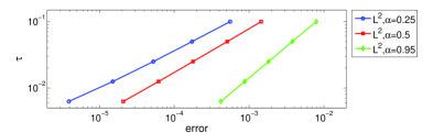
Figure 1. Numerical results for the case with a smooth solution at $t=1$ with $\beta=0.2$ and $\alpha=0.25,0.5,0.95$, discretized on a uniform mesh $h=2^{-10}$ and $\tau=0.2\times 2^{-k}$.

5.2. Homogeneous problems

In this part we present numerical results to illustrate the spatial convergence rates in Section 3. We performed numerical tests on the following three different initial data:

• Smooth data: $v(x)=\sin(2\pi x)$ which belongs to $H^{2}(\Omega)\cap H^{1}_{0}(\Omega)$.

• Nonsmooth data: $v(x)=\chi_{(0,1/2]}$ which lies in the space $\dot{H}^{\epsilon}(\Omega)$ for any $\epsilon\in[0,1/2)$.

• Very weak data: $v(x)=\delta_{1/2}(x)$, a Dirac $\delta_{1/2}(x)$-function concentrated at $x=1/2$, which belongs to the space $\dot{H}^{-\epsilon}(\Omega)$ for any $\epsilon\in(1/2,1]$.

In order to check the convergence rate of the semidiscrete scheme, we discretize the fractional derivatives with a small time step $\tau$ so that the temporal discretization error is negligible. In view of the possibly singular behavior as $t\rightarrow 0$, we set the time step $\tau$ to $\tau=t/(5\times 10^{4})$, with $t$ being the terminal time. For each example, we measure the error $e(t)=u(t)-u_{h}(t)$ by the normalized errors $\|e(t)\|_{L^{2}(\Omega)}/\|v\|_{L^{2}(\Omega)}$ and $\|\nabla e(t)\|_{L^{2}(\Omega)}/\|v\|_{L^{2}(\Omega)}$. The normalization enables us to observe the behavior of the error with respect to time in case of nonsmooth initial data.

5.2.1. Numerical results for example (2a): smooth initial data

The numerical results show $O(h^{2})$ and $O(h)$ convergence rates for the $L^{2}$- and $H^{1}$-norms of the error, respectively, for all three different $\alpha$ values, cf. Fig. 2. As the value of $\alpha$ increases from $0.25$ to $0.95$, the error at $t=1$ decreases accordingly, which resembles that for the single-term time-fractional diffusion equation [12].

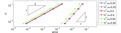
Figure 2. Numerical results for example (2a) at $t=1$ with $\beta=0.2$ and $\alpha=0.25$, $0.5$, $0.95$, discretized on a uniform mesh $h=2^{-k}$ and $\tau=2\times 10^{-5}$.

5.2.2. Numerical results for example (2b): nonsmooth initial data

For nonsmooth initial data, we are particularly interested in errors for $t$ close to zero, and thus we also present the errors at $t=0.01$ and $t=0.001$; see Table 2. The numerical results fully confirm the theoretically predicted rates for nonsmooth initial data. Further, in Table 3 we show the $L^{2}$-norm of the error for fixed $h=2^{-6}$ and $t\rightarrow 0$. We observe that the error deteriorates as $t\rightarrow 0$. Upon noting $v\in\dot{H}^{1/2-\epsilon}(\Omega)$, it follows from Theorem 3.2 that the error grows like $O(t^{-3\alpha/4})$, which agrees well with the results in Table 3.

Table 2. Numerical results for the nonsmooth case (2b) with $\alpha=0.5$ and $\beta=0.2$ at $t=1,0.01,0.001$, discretized on a uniform mesh with $h=2^{-k}$ and $\tau=t/(5\times 10^{4})$.

$t$	$k$	$3$	$4$	$5$	$6$	$7$	rate
$t=1$	$L^{2}$-norm	1.86e-3	4.64e-4	1.16e-4	2.87e-5	6.88e-6	$\approx 2.02$ ($2.00$)
	$H^{1}$-norm	4.89e-2	2.44e-2	1.22e-2	6.07e-3	2.96e-3	$\approx 1.01$ ($1.00$)
$t=0.01$	$L^{2}$-norm	8.04e-3	2.00e-3	5.01e-4	1.24e-4	2.98e-5	$\approx 2.03$ ($2.00$)
	$H^{1}$-norm	2.31e-2	1.16e-1	5.79e-2	2.88e-2	1.40e-2	$\approx 1.01$ ($1.00$)
$t=0.001$	$L^{2}$-norm	1.65e-2	4.14e-3	1.03e-3	2.56e-4	6.18e-4	$\approx 2.01$ ($2.00$)
	$H^{1}$-norm	5.15e-1	2.58e-1	1.29e-2	6.41e-2	3.13e-2	$\approx 1.01$ ($1.00$)

Table 3. $L^{2}$-error with $\alpha=0.5$ and $h=2^{-6}$ for $t\to 0$ for nonsmooth initial data (2b).

$t$	1e-3	1e-4	1e-5	1e-6	1e-7	1e-8	rate
Case(2b)	2.56e-4	5.39e-4	1.15e-3	2.91e-3	6.77e-3	1.55e-2	$\approx-0.37(-0.37)$

5.2.3. Numerical results for example (2c): very weak initial data

The numerical results show a superconvergence with a rate of $O(h^{2})$ in the $L^{2}$-norm and $O(h)$ in the $H^{1}$-norm, cf. Fig. 3(a). This is attributed to the fact that in one-dimension the solution with the Dirac $\delta$-function as the initial data is smooth from both sides of the support point and the finite element spaces $X_{h}$ have good approximation property. When the singularity point $x=1/2$ is not aligned with the grid, Fig. 3(b) indicates an $O(h^{3/2})$ and $O(h^{1/2})$ convergence rate for the $L^{2}$- and $H^{1}$-norm of the error, respectively, which agrees with our theory.

(a) $x=1/2$ aligns with the grid when $h=2^{-k}$

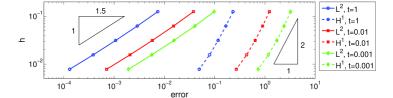
(b) $x=1/2$ does not align with the grid for $h=1/(2^{k}+1)$

Figure 3. Numerical results for very weak initial data: $\alpha=0.5$, $\beta=0.2$ at $t=0.005$, $0.01$, $1.0$, uniform mesh in time with $\tau=t/(5\times 10^{4})$.

5.3. Inhomogeneous problems

Now we consider the inhomogeneous problem with $v\equiv 0$ on the unit interval $\Omega=(0,1)$ and test the following two examples:

1. Nonsmooth data: $f(x,t)=(\chi_{[1/2,1]}(t)+1)\chi_{[0,{1/2}]}(x)$. The jump at $x=1/2$ leads to $f(t,\cdot)\notin\dot{H}^{1}(\Omega)$; nonetheless, for any $\epsilon>0$, $f\in L^{\infty}(0,T;\dot{H}^{{1/2}-\epsilon}(\Omega))$.

2. Very weak data: $f(x,t)=(\chi_{[1/2,1]}(t)+1)\delta_{1/2}(x)$ where $f$ involves a Dirac $\delta_{1/2}(x)$-function concentrated at $x=0.5$.

5.3.1. Numerical results for example (3a)

Since the errors are bounded independently of the time, cf. Theorem 3.3, we only present the errors in $L^{\infty}$ in time, i.e., $\|e(t)\|_{L^{2}(\Omega)}$ and $\|\nabla e(t)\|_{L^{2}(\Omega)}$. In Table 4, we present the $L^{2}$- and $H^{1}$-error at $t=1$, $0.01$, and $0.001$. The numerical results agree well with our theoretical predictions, i.e., $O(h^{2})$ and $O(h)$ convergence rates for the $L^{2}$- and $H^{1}$-norms of the error, respectively.

Table 4. Numerical results for example (3a) with $\alpha=0.5$ and $\beta=0.2$ at $t=1,0.01,0.001$, discretized on a uniform mesh $h=2^{-k}$ and $\tau=t/(5\times 10^{4})$.

$t$	$k$	$3$	$4$	$5$	$6$	$7$	rate
$t=1$	$L^{2}$-norm	1.76e-3	4.40e-4	1.10e-4	2.71e-5	6.53e-6	$\approx 2.01$ ($2.00$)
	$H^{1}$-norm	4.72e-2	2.36e-2	1.18e-2	5.86e-3	2.86e-3	$\approx 1.01$ ($1.00$)
$t=0.01$	$L^{2}$-norm	6.34e-4	1.59e-4	3.96e-5	9.82e-6	2.38e-6	$\approx 2.01$ ($2.00$)
	$H^{1}$-norm	1.89e-2	9.46e-3	4.72e-3	2.35e-3	1.15e-3	$\approx 1.01$ ($1.00$)
$t=0.001$	$L^{2}$-norm	4.55e-4	1.15e-4	2.88e-5	1.15e-6	1.73e-6	$\approx 2.02$ ($2.00$)
	$H^{1}$-norm	1.45e-2	7.31e-3	3.66e-3	1.82e-3	8.88e-4	$\approx 1.01$ ($1.00$)

5.3.2. Numerical results for example (3b)

In Table 6 we show convergence rates at three different times, i.e., $t=1$, $0.01$, and $0.001$. Here the mesh size $h$ is chosen to be $h=1/(2^{k}+1)$, and thus the support of the Dirac $\delta$-function does not align with the grid. The results indicate an $O(h^{1/2})$ and $O(h^{3/2})$ convergence rate for the $H^{1}$- and $L^{2}$-norm of the error, respectively, which agrees well with the theoretical prediction. If the Dirac $\delta$-function is supported at a grid point, both $L^{2}$- and $H^{1}$-norms of the error exhibit a superconvergence of one half order, cf. Table 5. This, however, theoretically remains to be established.

Table 5. Numerical results for example (3b) with $\alpha=0.5$ and $\beta=0.2$ at $t=0.1,0.01,0.001$, discretized on a uniform mesh $h=1/(2^{k}+1)$ and $\tau=t/(5\times 10^{4})$.

$t$	$k$	$3$	$4$	$5$	$6$	$7$	rate
$t=0.1$	$L^{2}$-norm	1.02e-2	4.01e-3	1.49e-3	5.35e-4	1.82e-4	$\approx 1.49$ ($1.50$)
	$H^{1}$-norm	3.24e-1	2.35e-1	1.65e-1	1.11e-1	6.94e-2	$\approx 0.50$ ($0.50$)
$t=0.01$	$L^{2}$-norm	4.66e-3	1.91e-3	7.29e-4	2.64e-4	9.02e-5	$\approx 1.45$ ($1.50$)
	$H^{1}$-norm	1.54e-1	1.14e-1	8.16e-2	5.54e-2	3.47e-2	$\approx 0.55$ ($0.50$)
$t=0.001$	$L^{2}$-norm	4.30e-3	1.83e-3	7.12e-4	2.61e-4	8.97e-5	$\approx 1.45$ ($1.50$)
	$H^{1}$-norm	1.47e-1	1.11e-1	8.05e-2	5.50e-2	3.45e-2	$\approx 0.55$ ($0.50$)

Table 6. Numerical results for example (3b) with $\alpha=0.5$ and $\beta=0.2$ at $t=1,0.01,0.001$, discretized on a uniform mesh with $h=2^{-k}$ and $\tau=t/(5\times 10^{4})$.

$t$	$k$	$3$	$4$	$5$	$6$	$7$	rate
$t=1$	$L^{2}$-norm	5.35e-4	1.34e-4	3.35e-5	8.31e-6	2.01e-6	$\approx 2.01$ ($1.50$)
	$H^{1}$-norm	1.49e-2	7.48e-3	3.74e-3	1.86e-3	9.07e-4	$\approx 1.01$ ($0.50$)
$t=0.01$	$L^{2}$-norm	6.67e-4	1.67e-4	4.17e-5	1.04e-5	2.52e-6	$\approx 2.03$ ($1.50$)
	$H^{1}$-norm	2.56e-2	1.29e-2	6.44e-3	3.20e-3	1.56e-3	$\approx 1.02$ ($0.50$)
$t=0.001$	$L^{2}$-norm	8.19e-4	2.08e-4	5.22e-5	1.30e-5	3.19e-6	$\approx 2.02$ ($1.50$)
	$H^{1}$-norm	3.96e-2	2.00e-2	1.00e-3	4.98e-3	2.45e-3	$\approx 1.01$ ($0.50$)

5.4. Examples in two-dimension

In this part, we present three two-dimensional examples on the unit square $\Omega=(0,1)^{2}$.

1. Nonsmooth initial data: $v=\chi_{(0,1/2)\times(0,1)}$ and $f\equiv 0$.

2. Very weak initial data: $v=\delta_{\Gamma}$ with $\Gamma$ being the boundary of the square $[1/4,3/4]^{2}$ and $\langle\delta_{\Gamma},\phi\rangle=\int_{\Gamma}\phi(s)\,ds$. By Hölder’s inequality and the continuity of the trace operator from $\dot{H}^{{1/2}+\epsilon}(\Omega)$ to $L^{2}(\Gamma)$ [2], we deduce $\delta_{\Gamma}\in H^{-1/2-\epsilon}(\Omega)$.

3. Nonsmooth right hand side: $f(x,t)=(\chi_{[1/20,1/10]}(t)+1)\chi_{(0,1/2)\times(0,1)}(x)$ and $v\equiv 0$.

To discretize the problem, we divide each direction into $N=2^{k}$ equally spaced subintervals, with a mesh size $h=1/N$ so that the domain $[0,1]^{2}$ is divided into $N^{2}$ small squares. We get a symmetric mesh by connecting the diagonal of each small square.

The numerical results for example (4a) are shown in Table 7, which agree well with Theorem 3.2, with a rate $O(h^{2})$ and $O(h)$, respectively, for the $L^{2}$- and $H^{1}$-norm of the error. Interestingly, for example (4b), both the $L^{2}$-norm and $H^{1}$-norm of the error exhibit super-convergence, cf. Table 8. The numerical results for example (4c) confirm the theoretical results; see Table 9. The solution profiles for examples (4b) and (4c) at $t=0.1$ are shown in Fig. 4, from which the nonsmooth region of the solution can be clearly observed.

Table 7. Numerical results for (4a) with $\alpha=0.5$ and $\beta=0.2$ at $t=0.1,0.01,0.001$, discretized on a uniform mesh, $h=2^{-k}$ and $\tau=t/10^{4}$.

$t$	$k$	$3$	$4$	$5$	$6$	$7$	rate
$t=0.1$	$L^{2}$-norm	5.25e-3	1.35e-3	3.38e-4	8.24e-5	1.98e-5	$\approx 2.06$ ($2.00$)
	$H^{1}$-norm	9.10e-2	4.53e-2	2.25e-2	1.09e-2	4.99e-3	$\approx 1.04$ ($1.00$)
$t=0.01$	$L^{2}$-norm	1.25e-2	3.23e-3	8.09e-4	1.97e-4	4.65e-5	$\approx 2.05$ ($2.00$)
	$H^{1}$-norm	2.18e-1	1.08e-1	5.35e-2	2.62e-2	1.27e-2	$\approx 1.05$ ($1.00$)
$t=0.001$	$L^{2}$-norm	3.02e-2	7.84e-3	1.97e-3	4.81e-4	1.16e-4	$\approx 2.03$ ($2.00$)
	$H^{1}$-norm	5.30e-1	2.64e-1	1.31e-1	6.38e-2	3.14e-2	$\approx 1.04$ ($1.00$)

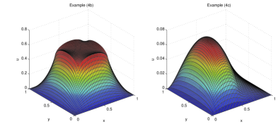
Figure 4. Numerical solutions of examples (4b) and (4c) with $h=2^{-6}$, $\alpha=0.5$, $\beta=0.2$ at $t=0.1$

Table 8. Numerical results for example (4b) with $\alpha=0.5$ and $\beta=0.2$ at $t=0.1,0.01,0.001$ for a uniform mesh with $h=2^{-k}$ and $\tau=t/10^{4}$.

$t$	$k$	$3$	$4$	$5$	$6$	$7$	rate
$t=0.1$	$L^{2}$-norm	1.18e-2	3.18e-3	8.41e-4	2.18e-4	5.41e-5	$\approx 1.92$ ($1.50$)
	$H^{1}$-norm	2.25e-1	1.13e-1	6.60e-2	3.40e-2	1.66e-2	$\approx 0.92$ ($0.50$)
$t=0.01$	$L^{2}$-norm	2.82e-2	7.62e-3	2.28e-3	5.26e-4	1.25e-4	$\approx 1.95$ ($2.00$)
	$H^{1}$-norm	5.66e-1	3.09e-1	1.65e-1	8.52e-2	4.19e-2	$\approx 0.94$ ($1.00$)
$t=0.001$	$L^{2}$-norm	6.65e-2	1.83e-3	4.98e-3	1.33e-3	3.30e-4	$\approx 1.91$ ($2.00$)
	$H^{1}$-norm	1.66e0	8.93e-1	4.75e-1	2.43e-1	1.21e-1	$\approx 0.95$ ($1.00$)

Table 9. Numerical results for example (4c) with $\alpha=0.5$ and $\beta=0.2$ at $t=0.1,0.01,0.001$ for a uniform mesh with $h=2^{-k}$ and $\tau=t/10^{4}$.

$t$	$k$	$3$	$4$	$5$	$6$	$7$	rate
$t=0.1$	$L^{2}$-norm	2.28e-3	5.86e-4	1.47e-4	3.58e-5	7.91e-6	$\approx 2.07$ ($2.00$)
	$H^{1}$-norm	3.97e-2	1.97e-2	9.77e-3	4.76e-3	2.13e-3	$\approx 1.06$ ($1.00$)
$t=0.01$	$L^{2}$-norm	1.06e-3	2.73e-4	6.86e-5	1.67e-6	3.70e-6	$\approx 2.06$ ($2.00$)
	$H^{1}$-norm	1.85e-2	9.18e-3	4.56e-3	2.22e-3	9.94e-3	$\approx 1.06$ ($1.00$)
$t=0.001$	$L^{2}$-norm	8.66e-4	2.28e-4	5.75e-5	1.40e-6	3.11e-6	$\approx 2.04$ ($2.00$)
	$H^{1}$-norm	1.56e-2	7.82e-3	3.88e-3	1.90e-3	8.47e-4	$\approx 1.05$ ($1.00$)

6. Concluding remarks

In this work, we have developed a simple numerical scheme based on the Galerkin finite element method for a multi-term time fractional diffusion equation which involves multiple Caputo fractional derivatives in time. A complete error analysis of the space semidiscrete Galerkin scheme is provided. The theory covers the practically very important case of nonsmooth initial data and right hand side. The analysis relies essentially on some new regularity results of the multi-term time fractional diffusion equation. Further, we have developed a fully discrete scheme based on a finite difference discretization of the Caputo fractional derivatives. The stability and error estimate of the fully discrete scheme were established, provided that the solution is smooth. The extensive numerical experiments in one- and two-dimension fully confirmed our convergence analysis: the empirical convergence rates agree well with the theoretical predictions for both smooth and nonsmooth data.

Appendix A Proof of Lemma 2.4

Proof.

First, we define an auxiliary function $v_{j}(t)$ by

$$\hat{v}_{j}(z)=\mathcal{L}(v_{j})=\frac{z^{\alpha-1}+\sum_{k=1}^{m}b_{k}z^{\alpha_{k}-1}}{z^{\alpha}+\sum_{k=1}^{m}b_{k}z^{\alpha_{k}}+\lambda_{j}}.$$

Now by the property of the Laplace transform $f(0^{+})=\lim_{z\to\infty}z\widehat{f}(z)$, we obtain $v_{j}(0+)=1$. The function $\bar{E}_{{\vec{\alpha}}}^{j}(t)$ is the inverse Laplace integral of $\widehat{\bar{E}_{{\vec{\alpha}}}^{j}}=(z^{\alpha}+\sum_{k=1}^{m}b_{k}z^{\alpha_{k}}+\lambda_{j})^{-1}$, i.e.

(A.1) $$\bar{E}_{{\vec{\alpha}}}^{j}(t)=\frac{1}{2\pi\mathrm{i}}\int_{Br}e^{zt}\frac{1}{{z^{\alpha}+\sum_{k=1}^{m}b_{k}z^{\alpha_{k}}+\lambda_{j}}}\,dz,$$

where $Br=\{z;\ \text{Re}~{}~{}z=\sigma,\ \sigma>0\}$ is the Bromwich path. The function $\widehat{\bar{E}_{{\vec{\alpha}}}^{j}}(z)$ has a branch point $0$, so we cut off the negative part of the real axis. Note that the function $z^{\alpha}+\sum_{k=1}^{m}b_{k}z^{\alpha_{k}}+\lambda_{j}$ has no zero in the main sheet of the Riemann surface including its boundaries on the cut. Indeed, if $z=\varrho e^{i\theta}$, with $\rho>0$, $\theta\in(-\pi,\pi)$, then

$$\Im\left\{z^{\alpha}+\sum_{k=1}^{m}b_{k}z^{\alpha_{k}}+\lambda_{j}\right\}=\varrho^{\alpha}\sin\alpha\theta+\sum_{k=1}^{m}b_{k}\varrho^{\alpha_{k}}\sin\alpha_{k}\theta\neq 0,\ \ \forall\theta\neq 0,$$

since $\sin\alpha\theta$ and $\sin\alpha_{k}\theta$ have the same sign for any $\theta\in(-\pi,\pi)$ and $b_{k}>0$. Hence, $\bar{E}_{{\vec{\alpha}}}^{j}(t)$ can be found by bending the Bromwich path into the Hankel path $Ha(\epsilon)$, which starts from $-\infty$ along the lower side of the negative real axis, encircles the disc $|s|=\epsilon$ counterclockwise and ends at $-\infty$ along the upper side of the negative real axis. Then by taking $\epsilon\to 0$, we obtain

$$\bar{E}_{{\vec{\alpha}}}^{j}(t)=\int_{0}^{\infty}e^{-rz}K_{n}(r)\,dr,$$

where

$$K_{n}(r)=-\frac{1}{\pi}\Im\left\{\left.\frac{1}{z^{\alpha}+\sum_{k=1}^{m}b_{k}z^{\alpha_{k}}+\lambda_{j}}\right|_{z=re^{i\pi}}\right\}.$$

It is easy to check

$$K_{n}(r)=\frac{1}{\pi}\frac{r^{\alpha}\sin\alpha\pi+\sum_{k=1}^{m}b_{k}r^{\alpha_{k}}\sin\alpha_{k}\pi}{(r^{\alpha}\cos\alpha\pi+\sum_{k=1}^{m}b_{k}r^{\alpha_{k}}\cos\alpha_{k}\pi+\lambda_{j})^{2}+(r^{\alpha}\sin\alpha\pi+\sum_{k=1}^{m}b_{k}r^{\alpha_{k}}\sin\alpha_{k}\pi)^{2}}$$

which is greater than zero for all $r>0$. Therefore, $\bar{E}_{{\vec{\alpha}}}^{j}(t)$ is completely monotone. A similar argument shows that $v_{j}(t)$ is also completely monotone. Consequently,

$$\int_{0}^{T}|\bar{E}_{{\vec{\alpha}}}^{j}(t)|\,dt=\int_{0}^{T}\bar{E}_{{\vec{\alpha}}}^{j}(t)\,dt=-\frac{1}{\lambda_{j}}\int_{0}^{T}v^{\prime}_{j}(t)\,dt=\frac{1}{\lambda_{n}}(1-v_{j}(T))<\frac{1}{\lambda_{n}},$$

which concludes the proof of the lemma. ∎

References

• [1] E. E. Adams and L. W. Gelhar. Field study of dispersion in a heterogeneous aquifer: 2. spatial moments analysis. Water Res. Research, 28(12):3293–3307, 1992.
• [2] R. Adams and J. Fournier. Sobolev Spaces. Elsevier/Academic Press, Amsterdam, 2003.
• [3] H. Brunner, L. Ling, and M. Yamamoto. Numerical simulations of 2D fractional subdiffusion problems. J. Comput. Phys., 229(18):6613 –6622, 2010.
• [4] E. Casas, C. Clason, and K. Kunisch. Parabolic control problems in measure spaces with sparse solutions. SIAM J. Control Optim., 51(1):28–63, 2013.
• [5] E. Casas and E. Zuazua. Spike controls for elliptic and parabolic PDEs. Systems Control Lett., 62(4):311–318, 2013.
• [6] A. M. A. El-Sayed, I. L. El-Kalla, and E. A. A. Ziada. Analytical and numerical solutions of multi-term nonlinear fractional orders differential equations. Appl. Numer. Math., 60(8):788–797, 2010.
• [7] Z.-J. Fu, W. Chen, and H.-T. Yang. Boundary particle method for Laplace transformed time fractional diffusion equations. J. Comput. Phys., 235:52–66, 2013.
• [8] S. B. Hadid and Y. F. Luchko. An operational method for solving fractional differential equations of an arbitrary real order. Panamer. Math. J., 6(1):57–73, 1996.
• [9] H. Jiang, F. Liu, I. Turner, and K. Burrage. Analytical solutions for the multi-term time-space Caputo-Riesz fractional advection-diffusion equations on a finite domain. J. Math. Anal. Appl., 389(2):1117–1127, 2012.
• [10] B. Jin, R. Lazarov, J. Pasciak, and Z. Zhou. Error analysis of semidiscrete finite element methods for inhomogeneous time-fractional diffusion. preprint, arXiv:1307.1068, 2013.
• [11] B. Jin, R. Lazarov, J. Pasciak, and Z. Zhou. Galerkin fem for fractional order parabolic equations with initial data in $H^{-s},~{}0\leq s\leq 1$. Proc. 5th Conf. Numer. Anal. Appl., Springer, 24–37, 2013.
• [12] B. Jin, R. Lazarov, and Z. Zhou. Error estimates for a semidiscrete finite element method for fractional order parabolic equations. SIAM J. Numer. Anal., 51(1):445–466, 2013.
• [13] B. Jin and X. Lu. Numerical identification of a Robin coefficient in parabolic problems. Math. Comp., 81:1369–1398, 2012.
• [14] B. Jin and W. Rundell. An inverse problem for a one-dimensional time-fractional diffusion problem. Inverse Problems, 28(7):075010, 19, 2012.
• [15] J. Katsikadelis. Numerical solution of multi-term fractional differential equations. ZAMM Z. Angew. Math. Mech., 89(7):593–608, 2009.
• [16] J. F. Kelly, R. J. McGough, and M. M. Meerschaert. Analytical time-domain Green’s functions for power-law media. J. Acoust. Soc. Am., 124(5):2861–2872, 2008.
• [17] A. Kilbas, H. Srivastava, and J. Trujillo. Theory and Applications of Fractional Differential Equations. Elsevier, Amsterdam, 2006.
• [18] X. Li and C. Xu. A space-time spectral method for the time fractional diffusion equation. SIAM J. Numer. Anal., 47(3):2108–2131, 2009.
• [19] Z. Li, Y. Liu, and M. Yamamoto. Initial-boundary value problems for multi-term time-fractional diffusion equations with positive constant coefficients. preprint, arXiv:1312.2112, 2013.
• [20] Z. Li and M. Yamamoto. Initial-boundary value problems for linear diffusion equations with multiple time-fractional derivatives. preprint, arXiv:1306.2778, 2013.
• [21] Y. Lin and C. Xu. Finite difference/spectral approximations for the time-fractional diffusion equation. J. Comput. Phys., 225(2):1533–1552, 2007.
• [22] F. Liu, M. M. Meerschaert, R. J. McGough, P. Zhuang, and X. Liu. Numerical methods for solving the multi-term time-fractional wave-diffusion equation. Frac. Cal. Appl. Anal., 16(1):9–25, 2013.
• [23] Y. Luchko. Initial-boundary-value problems for the generalized multi-term time-fractioal diffusion equations. J. Math. Anal. Appl., 374(2):538–548, 2011.
• [24] Y. Luchko and R. Gorenflo. An operational method for solving fractional differential equations with the Caputo derivatives. Acta Math. Vietnam., 24(2):207–233, 1999.
• [25] W. McLean and V. Thomée. Maximum-norm error analysis of a numerical solution via Laplace transformation and quadrature of a fractional-order evolution equation. IMA J. Numer. Anal., 30(1):208–230, 2010.
• [26] R. Metzler, J. Klafter, and I. M. Sokolov. Anomalous transport in external fields: Continuous time random walks and fractional diffusion equations extended. Phys. Rev. E, 58(2):1621–1633, 1998.
• [27] K. Mustapha. An implicit finite-difference time-stepping method for a sub-diffusion equation, with spatial discretization by finite elements. IMA J. Numer. Anal., 31(2):719–739, 2011.
• [28] K. Mustapha and W. McLean. Superconvergence of a discontinuous Galerkin method for fractional diffusion and wave equations. SIAM J. Numer. Anal., 51(1):491–515, 2013.
• [29] R. Nigmatulin. The realization of the generalized transfer equation in a medium with fractal geometry. Phys. Stat. Sol. B, 133:425–430, 1986.
• [30] K. Sakamoto and M. Yamamoto. Initial value/boundary value problems for fractional diffusion-wave equations and applications to some inverse problems. J.Math.Anal.Appl., 382(1):426–447, 2011.
• [31] R. Schumer, D. A. Benson, M. M. Meerschaert, and B. Baeumer. Fractal mobile/immobile solute transport. Water Res. Research., 39(10):1296, 13 pp., 2003.
• [32] V. Thomée. Galerkin Finite Element Methods for Parabolic Problems, volume 25 of Springer Series in Computational Mathematics. Springer-Verlag, Berlin, 2006.
• [33] J. Xie and J. Zou. Numerical reconstruction of heat fluxes. SIAM J. Numer. Anal., 43(4):1504–1535, 2005.
• [34] M. Zayernouri and G. E. Karniadakis. Exponentially accurate spectral and spectral element methods for fractional ODEs. J. Comput. Phys., 257, Part A:460– 480, 2014.
• [35] Y.-N. Zhang, Z.-Z. Sun, and H.-W. Wu. Error estimates of Crank-Nicolson-type difference schemes for the subdiffusion equation. SIAM J. Numer. Anal., 49(6):2302–2322, 2011.
• [36] J. Zhao, J. Xiao, and Y. Xu. Stability and convergence of an effective finite element method for multiterm fractional partial differential equations. Abstr. Appl. Anal., pages Art. ID 857205, 10, 2013.