Preserving Lagrangian structure in
nonlinear model reduction with
application to structural dynamics

Abstract

This work proposes a model-reduction methodology that preserves Lagrangian structure (equivalently Hamiltonian structure) and achieves computational efficiency in the presence of high-order nonlinearities and arbitrary parameter dependence. As such, the resulting reduced-order model retains key properties such as energy conservation and symplectic time-evolution maps. We focus on parameterized simple mechanical systems subjected to Rayleigh damping and external forces, and consider an application to nonlinear structural dynamics. To preserve structure, the method first approximates the system’s ‘Lagrangian ingredients’—the Riemannian metric, the potential-energy function, the dissipation function, and the external force—and subsequently derives reduced-order equations of motion by applying the (forced) Euler–Lagrange equation with these quantities. From the algebraic perspective, key contributions include two efficient techniques for approximating parameterized reduced matrices while preserving symmetry and positive definiteness: matrix gappy POD and reduced-basis sparsification (RBS). Results for a parameterized truss-structure problem demonstrate the importance of preserving Lagrangian structure and illustrate the proposed method’s merits: it reduces computation time while maintaining high accuracy and stability, in contrast to existing nonlinear model-reduction techniques that do not preserve structure.

1 Introduction

Computational modeling and simulation for simple mechanical systems characterized by a Lagrangian formalism has become indispensable across a variety of industries. Such simulations enable the understanding of complex systems, reduced design costs, and improved reliability for a wide range of applications. For example, computational structural dynamics tools have become widely used in applications ranging from aerospace to biomedical-device design; molecular-dynamics simulations have gained popularity in materials science and biology, in particular. However, the high computational cost incurred by simulating large-scale simple mechanical systems can result in simulation times on the order of weeks, even when using high-performance computers. As a result, these simulation tools are impractical for time-critical applications that demand the accuracy provided by large-scale, high-fidelity models. In particular, applications such as nondestructive evaluation for structural health monitoring, multiscale modeling, embedded control, design optimization, and uncertainty quantification require highly accurate results to be obtained quickly.

In this work, we consider models that depend on a set of parameters, e.g., design variables, operating conditions. In this context, model-reduction methods present a promising approach for addressing time-critical problems. During the offline stage, these methods perform computationally expensive ‘training’ tasks, which may include evaluating the high-fidelity model for several instances of the system parameters and computing a low-dimensional subspace for the solution. Then, during the inexpensive online stage, these methods quickly compute approximate solutions for arbitrary values of the system parameters. To accomplish this, they reduce the dimension of the high-fidelity model by restricting solutions to lie in the low-dimensional subspace that was computed offline; they also introduce other approximations when nonlinearities are present. Thus, the reduced-order model used online is characterized by a low-dimensional dynamical system that arises from a projection process on the high-fidelity-model equations. This offline/online strategy is effective primarily in two scenarios: ‘many query’ problems (e.g., Bayesian inference), where the high offline cost is amortized over many online evaluations, and real-time problems (e.g., control) characterized by stringent constraints on online evaluation time.

Generating a reduced-order model that preserves the Lagrangian structure intrinsic to mechanical systems is not a trivial task. Such structure is critical to preserve, as it leads to fundamental properties such as energy conservation (in the absence of non-conservative forces), conservation of quantities associated with symmetries in the system, and symplectic time-evolution maps. In fact, the class of structure-preserving time integrators (e.g., geometric integrators [15], variational integrators [19]) has been developed to ensure that the discrete solution to the high-fidelity computational model associates with the time-evolution map of a (modified) Lagrangian system.

Lall et al. [18] show that performing a Galerkin projection on the Euler–Lagrange equation—as opposed to the first-order state-space form—leads to a reduced-order model that preserves Lagrangian structure. However, the computational cost of assembling the associated low-dimensional equations of motion scales with the dimension of the high-fidelity model. For this reason, this approach is efficient only when the low-dimensional operators can be assembled a priori; this occurs only in very limited cases e.g., when operators have a low-order polynomial dependence on the state and are affine in functions of the parameters [22].

Several methods have been developed in the context of nonlinear-ODE model reduction that can reduce the computational cost of assembling the low-dimensional equations of motion. However, these methods destroy Lagrangian structure when applied to simple mechanical systems. For example, collocation approaches [4, 23] perform a Galerkin projection on only a small subset of the full-order equations characterizing the high-fidelity model. Although this method works well for some nonlinear ODEs, it destroys Lagrangian structure. The discrete empirical interpolation method (DEIM) [9, 14, 11] and gappy proper orthogonal decomposition (POD) reconstruction methods [13, 6, 7] compute a few entries of the vector-valued nonlinear functions, and then approximate the uncomputed entries by interpolation or least-squares regression using an empirically derived basis. Galerkin projection can then be performed with the approximated nonlinear function. Again, this technique destroys Lagrangian structure.

The goal of this work is to devise a reduced-order model for nonlinear simple mechanical systems with general parameter dependence that leads to computationally inexpensive online solutions and preserves Lagrangian structure. We focus particularly on parameterized structural-dynamics models under Rayleigh damping and external forces. The methodology we propose constructs a reduced-order model by first approximating the ‘Lagrangian ingredients’ (i.e., quantities defining the problem’s Lagrangian structure) and subsequently deriving the equations of motion by applying the Euler–Lagrange equation to these ingredients. The method approximates the Lagrangian ingredients as follows:

1. Configuration space. The low-dimensional configuration space is derived using standard dimension-reduction techniques, e.g., proper orthogonal decomposition, modal decomposition.

2. Riemannian metric. The Riemannian metric is defined by a low-dimensional symmetric positive-definite matrix. We propose two efficient methods for approximating this low-dimensional matrix that preserve symmetry and positive definiteness.

3. Potential-energy function. The potential energy function is approximated by employing the original potential-energy function, but with the low-dimensional reduced-basis matrix replaced by a low-dimensional sparse matrix with only a few nonzero rows. This sparse matrix is computed online by matching the gradient of the reduced potential to first order about the equilibrium configuration.

4. Dissipation function. The damping matrix associated with the Rayleigh dissipation function is a linear combination of the mass matrix (which defines the Riemannian metric) and the Hessian of the potential. Thus, we form the approximated Rayleigh dissipation function in the same fashion, but employ the approximated mass matrix from ingredient II and approximated potential from ingredient III.

5. External force. The external force is derived by applying the Lagrange–D’Alembert principle with variations in the configuration space. We approximate this by applying gappy POD reconstruction to the external force as expressed in the original coordinates. As a result, the external force appearing in the reduced-order equations of motion can be derived by applying the Lagrange–D’Alembert principle to this modified external force with variations restricted to the low-order configuration space.

We note that a structure-preserving method [5] has been recently proposed for nonlinear port-Hamiltonian systems, which are generalizations of Hamiltonian systems. While this technique guarantees that properties such as stability and passivity are preserved, it does not in fact preserve Lagrangian or classical Hamiltonian structure. In particular, the resulting reduced-order equations of motion cannot be derived from approximated ingredients such as those enumerated above; as a consequence, the approach does not ensure symplecticity or energy conservation for conservative systems, for example.

As hinted above, preserving structure for Lagrangian ingredient II is equivalent to efficiently approximating a low-dimensional reduced matrix while preserving symmetry and positive definiteness. This algebraic task is relevant to a broad scope of applications, e.g., approximating extreme eigenvalues/eigenvectors of a parameterized matrix, preserving Hessian positive definiteness in optimization algorithms. For this reason, Section 2 presents approximation techniques for Lagrangian ingredient II in a stand-alone algebraic setting that does not rely on the Lagrangian formalism. Similarly, Section 3 considers Lagrangian ingredient III in a purely alegraic context that does not depend on Lagrangian dynamics.

The remainder of the paper is organized as follows. Section 4 introduces the Lagrangian-mechanics formulation. Section 5 outlines existing model-reduction techniques and highlights the need for an efficient, structure-preserving method. Section 6 presents the proposed method. Section 7 presents numerical experiments applied to a simple mechanical system from structural dynamics. Finally, Section 8 summarizes the contributions and suggests further research.

The structure-preserving model-reduction methods proposed in this work also preserve Hamiltonian structure when the Hamiltonian formulation of classical mechanics is used. Appendix A provides this connection.

2 Preserving matrix symmetry and positive definiteness

This section presents approximation techniques for Lagrangian ingredient II in an algebraic setting. First, to establish notation, denote the system parameters by ${\mu}\in\mathcal{D}$, where $\mathcal{D}$ represents the parameter domain. Let ${\mathbf{A}\left({\mu}\right)}$ denote an $N\times N$ parameterized symmetric positive-definite (possibly dense) matrix. Finally, let ${\mathbf{V}}$ denote a dense, parameter-independent, full-column-rank $N\times n$ matrix with $n\ll N$ whose columns can be interpreted as a reduced basis spanning an $n$-dimensional subspace of $\mathbb{R}^{N}$. We consider the following online problem:

• At a cost independent of $N$, compute a symmetric positive-definite matrix ${\tilde{\mathbf{A}}\left({\mu}^{\star}\right)}$ that is appropriately close to the matrix ${\mathbf{V}}^{T}{\mathbf{A}\left({\mu}^{\star}\right)}{\mathbf{V}}$ for any specified online point ${\mu}^{\star}\in\mathcal{D}$.

Note that due to the density of ${\mathbf{V}}$, directly computing ${\mathbf{V}}^{T}{\mathbf{A}\left({\mu}^{\star}\right)}{\mathbf{V}}$ requires computing all $\mathcal{O}(N)$ entries of the matrix ${\mathbf{A}\left({\mu}^{\star}\right)}$. Recall that the offline/online strategy we adopt permits expensive offline operations that facilitate the solution to online problem (P1). These operations may include collecting $p$ ‘snapshots’ of the matrix ${\mathbf{A}\left({\mu}^{i}\right)}$, $i=1,\ldots,p$, where ${\mu}^{i}\in\mathcal{D}$ denotes the $i$th instance of the training set.

We assume that computing a single entry of ${\mathbf{A}\left({\mu}^{\star}\right)}$ for any specified online point ${\mu}^{\star}\in\mathcal{D}$ is inexpensive, i.e., the number of floating-point operations (flops) is independent of $N$. However, we make no other assumptions regarding the parameters or the matrix. In particular, we do not assume affine parametric dependence of the matrix, and we view ${\mu}\mapsto{\mathbf{A}\left({\mu}\right)}$ simply as a mechanism for generating instances of the matrix $\mathbf{A}$.

We now present two methods for solving online problem (P1). Method 1 approximates the reduced matrix by projecting the full matrix onto a sparse basis, while Method 2 approximates the reduced matrix as a linear combination of pre-computed reduced matrices. Later, Section 5.2 constrasts the proposed methods with existing model reduction approaches such as DEIM, gappy POD, and collocation. These existing methods apply a one-sided sampling operator to the matrix, i.e., they replace ${\mathbf{V}}^{T}$ with some type of sparse matrix. While this leads to an inexpensive approximation, it gives rise to a non-symmetric reduced matrix approximation. This destroys the underlying problem structure and therefore fails to meet the requirements of online problem (P1).

2.1 Reduced-basis sparsification (RBS)

We first consider a strategy that ‘injects sparseness’ into the matrix ${\mathbf{V}}$. That is, we replace ${\mathbf{V}}$ by ${{\mathbf{U}}_{\mathbf{A}}}\in\mathbb{R}^{N\times n}$, which has full column rank and only $m$ rows (with $n\leq m\ll N$) containing nonzero entries:

$$\tilde{\mathbf{A}}\left({\mu}\right) ={{\mathbf{U}}_{\mathbf{A}}}^{T}{\mathbf{A}\left({\mu}\right)}{{\mathbf{U}}_{\mathbf{A}}}.$$ (1)

This sparse matrix may be expressed as ${{\mathbf{U}}_{\mathbf{A}}}\equiv{\mathbf{P}}\underline{{{\mathbf{U}}_{\mathbf{A}}}}$, where ${\mathbf{P}}\in\{0,1\}^{N\times m}$ is a ‘sampling matrix’ consisting of $m$ selected columns of the $N\times N$ identity matrix, $\underline{{{\mathbf{U}}_{\mathbf{A}}}}\in\mathbb{R}^{m\times n}_{*}$ is a dense matrix with full column rank $n$, and $\mathbb{R}^{m\times n}_{*}$ denotes the noncompact Stiefel manifold: the set of full-rank $m\times n$ matrices. Clearly, $\tilde{\mathbf{A}}\left({\mu}\right)$ is symmetric positive definite if ${\mathbf{A}\left({\mu}\right)}$ is symmetric positive definite; thus, the approximation defined by (1) preserves the requisite structure. Note that this approximation will also preserve structure in cases where ${\mathbf{A}\left({\mu}\right)}$ is symmetric positive semidefinite or simply symmetric. Further, the (online) operation count for computing $\tilde{\mathbf{A}}\left({\mu}^{\star}\right)$ for online point ${\mu}^{\star}\in\mathcal{D}$ is independent of $N$. Computing ${{\mathbf{P}}^{T}}{\mathbf{A}\left({\mu}^{\star}\right)}{\mathbf{P}}$ is equivalent to computing only $m^{2}$ (symmetric) entries of ${\mathbf{A}\left({\mu}^{\star}\right)}$ and entails $\mathcal{O}(m^{2})$ flops; subsequently computing ${\tilde{\mathbf{A}}\left({\mu}^{\star}\right)}=\underline{{{\mathbf{U}}_{\mathbf{A}}}}^{T}\left[{{\mathbf{P}}^{T}}{\mathbf{A}\left({\mu}^{\star}\right)}{\mathbf{P}}\right]\underline{{{\mathbf{U}}_{\mathbf{A}}}}$ requires $\mathcal{O}(m^{2}n+mn^{2})$ flops.

Given a sampling matrix ${\mathbf{P}}$, the matrix $\underline{{{\mathbf{U}}_{\mathbf{A}}}}$ can be computed offline to minimize the average approximation error over the snapshots, i.e., according to the following optimization problem:

$$\underline{{{\mathbf{U}}_{\mathbf{A}}}}=\arg\min_{\mathbf{X}\in\mathbb{R}^{m\times n}_{*}}\sum_{i=1}^{p}\bigl{\|}\mathbf{X}^{T}{{\mathbf{P}}^{T}}{\mathbf{A}\left({\mu}^{i}\right)}{\mathbf{P}}\mathbf{X}-{\mathbf{V}}^{T}{\mathbf{A}\left({\mu}^{i}\right)}{\mathbf{V}}\bigr{\|}_{F}^{2},$$ (2)

where the subscript $F$ denotes the Frobenius norm. To handle the fact that $\mathbb{R}^{m\times n}_{*}$ is an open set, optimization problem (2) can first be solved over $\mathbb{R}^{m\times n}$ and the solution can be subsequently projected onto $\mathbb{R}^{m\times n}_{*}$, which is analogous to the approach taken by Vandereycken [25, Algorithm 6]. We note that other objective functions may be considered for specialized online analyses, e.g., the approximation error of extreme eigenvalues or eigenvectors over the matrix snapshots. Note that problem (2) is a small-scale optimization problem, as $m,n\ll N$. It can be solved at a cost independent of $N$ (for each optimization iteration) during the offline stage after the matrix snapshots ${\mathbf{A}\left({\mu}^{i}\right)}$, $i=1,\ldots,p$ and their reduced counterparts ${\mathbf{V}}^{T}{\mathbf{A}\left({\mu}^{i}\right)}{\mathbf{V}}$, $i=1,\ldots,p$ have been computed.

Procedure 1 provides the offline and online steps required to implement the RBS approximation.

Offline stage

1 Collect matrix snapshots ${\mathbf{A}\left({\mu}^{i}\right)}$, $i=1,\ldots,p$.

2 Form reduced the matrices ${\mathbf{V}}^{T}{\mathbf{A}\left({\mu}^{i}\right)}{\mathbf{V}}$, $i=1,\ldots,p$.

3 Choose the sample matrix ${\mathbf{P}}$.

4 Determine $\underline{{{\mathbf{U}}_{\mathbf{A}}}}$ as the solution to problem (2).

Online stage (given ${\mu}^{\star}$)

1 Compute ${{\mathbf{P}}^{T}}{\mathbf{A}\left({\mu}^{\star}\right)}{\mathbf{P}}$.

2 Form ${\tilde{\mathbf{A}}\left({\mu}^{\star}\right)}=\underline{{{\mathbf{U}}_{\mathbf{A}}}}^{T}\left[{{\mathbf{P}}^{T}}{\mathbf{A}\left({\mu}^{\star}\right)}{\mathbf{P}}\right]\underline{{{\mathbf{U}}_{\mathbf{A}}}}$.

Procedure 1 Reduced-basis sparsification for symmetric matrices

Remark 2.1.

This paper does not focus on methods for selecting the sampling matrix ${\mathbf{P}}$, a task that is typically carried out during the offline stage and uses the collected snapshots. All numerical experiments presented in Section 7 use the GNAT greedy approach [6] for this purpose. This method has proven to be quite robust, even when applied to the approximation techniques proposed in this paper. A more careful study of sampling algorithms will be addressed in future work, where ideas of tailoring the sampling approach to the specific reduced-order modeling approximation will be explored.

2.1.1 Exactness conditions

In the full-sampling case where $m=N$, the approximation is exact if problem (2) is solved via a gradient-based method with an initial guess of $\mathbf{X}^{(0)}={{\mathbf{P}}^{T}}{\mathbf{V}}$; we do this in practice. Under these conditions, ${{\mathbf{U}}_{\mathbf{A}}}={\mathbf{V}}$ and so $\tilde{\mathbf{A}}\left({\mu}\right)={\mathbf{V}}^{T}{\mathbf{A}\left({\mu}\right)}{\mathbf{V}}$.

In the general case where $m<N$, it is possible to show that the approximation is exact if the matrix is parameter-independent (i.e., ${\mathbf{A}\left({\mu}\right)}=\mathbf{A}$) and $m\geq n$. This situation is considered in the discussion that follows Theorem 2.2 below. It is also possible to prove a more general exactness result in cases where the parametric dependence of ${\mathbf{A}\left({\mu}\right)}$ is relatively simple. In particular, consider the parametric form

$${\mathbf{A}\left({\mu}\right)}={{{h}_{1}}\left({\mu}\right)}~{}{\mathbf{A}_{1}}+{{{h}_{2}}\left({\mu}\right)}~{}{\mathbf{A}_{2}},$$ (3)

where ${\mathbf{A}_{1}}$ and ${\mathbf{A}_{2}}$ are $N\times N$ symmetric positive-definite matrices and ${{h}_{1}},{{h}_{2}}:\mathcal{D}\rightarrow\mathbb{R}$. It can then be shown that a sparse reduced basis exists that exactly captures ${\mathbf{V}}^{T}{\mathbf{A}\left({\mu}\right)}{\mathbf{V}}$ under conditions related to how well the eigenvalues of the sampled matrix ${{\mathbf{P}}^{T}}\mathbf{A}({\mu}){\mathbf{P}}$ encompass (or surround) those of the reduced matrix ${\mathbf{V}}^{T}\mathbf{A}({\mu}){\mathbf{V}}$. Loosely stated, the encompassing conditions amount to how well the sampled matrix captures the behavior of the reduced matrix. Formally, the following theorem makes precise the notion of encompassing using eigenvalue interlacing ideas from classical linear algebra.

Theorem 2.2.

Let ${\mathbf{A}\left({\mu}\right)}$ have the form given by Eq. (3). Then,

$$\exists~{}\underline{{{\mathbf{U}}_{\mathbf{A}}}}\in\mathbb{R}^{m\times n}~{}~{}\mbox{such that}~{}~{}~{}\underline{{{\mathbf{U}}_{\mathbf{A}}}}^{T}\hskip 1.8063pt{{\mathbf{P}}^{T}}\hskip 1.8063pt{\mathbf{A}\left({\mu}\right)}\hskip 1.8063pt{\mathbf{P}}\hskip 1.8063pt\underline{{{\mathbf{U}}_{\mathbf{A}}}}={\mathbf{V}}^{T}\hskip 1.8063pt{\mathbf{A}\left({\mu}\right)}\hskip 1.8063pt{\mathbf{V}},\quad\forall{\mu}\in\mathcal{D}$$ (4)

if and only if the generalized eigenvalues of $({\mathbf{V}}^{T}{\mathbf{A}_{2}}{\mathbf{V}},{\mathbf{V}}^{T}{\mathbf{A}_{1}}{\mathbf{V}})$ interlace the generalized eigenvalues of $({{\mathbf{P}}^{T}}{\mathbf{A}_{2}}{\mathbf{P}},{{\mathbf{P}}^{T}}{\mathbf{A}_{1}}{\mathbf{P}})$, i.e.,

$$\lambda^{(s)}_{i}\leq\lambda^{(r)}_{i}\leq\lambda^{(s)}_{i+m-n}~{}~{}~{}for~{}i=1,...,n,$$ (5)

with

$$\left[{\mathbf{V}}^{T}{\mathbf{A}_{2}}{\mathbf{V}}\right]\mathbf{x}_{i}^{(r)}=\lambda_{i}^{(r)}\left[{\mathbf{V}}^{T}{\mathbf{A}_{1}}{\mathbf{V}}\right]\mathbf{x}_{i}^{(r)},\quad i=1,\ldots n$$

and

$$\left[{{\mathbf{P}}^{T}}{\mathbf{A}_{2}}{\mathbf{P}}\right]\mathbf{x}_{i}^{(s)}=\lambda_{i}^{(s)}\left[{{\mathbf{P}}^{T}}{\mathbf{A}_{1}}{\mathbf{P}}\right]\mathbf{x}_{i}^{(s)},\quad i=1,\ldots,m.$$

Note that the eigenvalues are sorted in order of increasing magnitude.

Appendix D.1 contains the proof. Here, we discuss the theorem’s implications.

When $\mathbf{A}$ is independent of ${\mu}$, we can choose ${{h}_{1}}={{h}_{2}}=1$ and ${\mathbf{A}_{1}}={\mathbf{A}_{2}}$. The interlacing property is then trivially satisfied for $m=n$ with $\lambda^{(s)}_{i}=\lambda^{(r)}_{i}=1$, and so the equality in (4) always holds. When instead ${\mathbf{A}_{1}}\neq{\mathbf{A}_{2}}$ and $m\hskip-2.8903pt=\hskip-2.8903ptn\hskip-2.8903pt+\hskip-2.8903pt1$, the interlacing definition is quite restrictive, as it implies that $\lambda^{(s)}_{k}\leq\lambda^{(r)}_{k}\leq\lambda^{(s)}_{k+1}$. We would not generally expect the eigenvalues of the sampled and reduced matrices to have this property. However, when $m\gg n+1$, each interval width is (much) larger and so the condition is not nearly as restrictive. For example, if $n=100$ and $m=300$, then interlacing implies that $\lambda^{(s)}_{i}\leq\lambda^{(r)}_{i}\leq\lambda^{(s)}_{i+200}$. Thus, we generally expect the conditions of the theorem to be satisfied for sufficiently large $m$, though this is not guaranteed and depends on matrix spectrum. As a final note, although the theorem assumes a specific form of ${\mathbf{A}\left({\mu}\right)}$, it should characterize the rough behavior of a more general ${\mathbf{A}\left({\mu}\right)}$ that does not vary ‘too much’ from the affine functional form (3).

2.2 Matrix gappy POD

An alternative structure-preserving approximation applicable to problem (P1) assumes the following form:

$$\tilde{\mathbf{A}}\left({\mu}\right) =\sum\limits_{i=1}^{n_{\mathbf{A}}}{{\xi_{\mathbf{A}}^{i}}\left({\mu}\right)}{\mathbf{V}}^{T}{\underline{\mathbf{A}}}_{i}{\mathbf{V}}.$$ (6)

Here, the matrices ${\underline{\mathbf{A}}}_{i}$, $i=1,\ldots,{n_{\mathbf{A}}}$ are $N\times N$ symmetric matrices that are computed offline and define a basis for the matrix ${\mathbf{A}\left({\mu}\right)}$. Due to the symmetry of ${\underline{\mathbf{A}}}_{i}$, $i=1,\ldots,{n_{\mathbf{A}}}$, the approximation $\tilde{\mathbf{A}}\left({\mu}\right)$ will always be symmetric. The parameter-dependent coefficients $\xi_{\mathbf{A}}\equiv\left(\xi_{\mathbf{A}}^{1},\ldots,\xi_{\mathbf{A}}^{{n_{\mathbf{A}}}}\right)$ are computed online in an efficient manner that ensures $\tilde{\mathbf{A}}\left({\mu}\right)$ is positive definite and thereby preserves requisite structure.

The next sections describe procedures for computing the matrix basis and coefficients. We refer to this method as ‘matrix gappy POD’, as it amounts to the gappy POD procedure [13] applied to matrix data with modifications to preserve positive definiteness. The approach, which we originally proposed [8], is a more general formulation of the ‘matrix DEIM’ approach [26] (or ‘multi-component EIM’ [24] in the context of the reduced-basis method applied to parametrized non-affine elliptic PDEs), as it permits least-squares reconstruction (not simply interpolation). Further, it is equipped with a mechanism to maintain positive definiteness.

2.2.1 Offline computation: matrix basis

To obtain the matrix basis, we propose applying a vectorized POD method, wherein the basis can be considered a set of ‘principal matrices’ that optimally represent the matrix $\mathbf{A}$ over the training set $\{{\mu}^{i}\}$. The (offline) steps for this method are as follows:

1. Collect matrix snapshots ${\mathbf{A}\left({\mu}^{i}\right)}$, $i=1,\ldots,p$.

2. Vectorize the snapshots $\mathbf{a}^{i}\equiv v\left({\mathbf{A}\left({\mu}^{i}\right)}\right)\in\mathbb{R}^{N^{2}}$, $i=1,\ldots,p$, where the function $v:\mathbb{R}^{N\times N}\rightarrow\mathbb{R}^{N^{2}}$ vectorizes a matrix.

3. Compute an ${n_{\mathbf{A}}}$-dimensional (with ${n_{\mathbf{A}}}\leq p$) POD basis of the vectorized snapshots

   $${{\mathbf{W}}_{\mathbf{a}}}\equiv\left[{\underline{\mathbf{a}}}^{1}\ \cdots\ {\underline{\mathbf{a}}}^{{n_{\mathbf{A}}}}\right]\in\mathbb{R}^{N^{2}\times{n_{\mathbf{A}}}}$$ (7)

   using vectorized snapshots $\{\mathbf{a}^{i}\}_{i=1}^{p}$ and an ‘energy criterion’ $\eta_{\mathbf{A}}\in\left[0,1\right]$ as inputs to Algorithm 5 of Appendix B.

4. Transform these POD basis vectors into their matrix counterparts:

   $${\underline{\mathbf{A}}}_{i}=v^{-1}\left({\underline{\mathbf{a}}^{i}}\right),\quad i=1,\ldots,{n_{\mathbf{A}}}.$$ (8)

Each matrix ${\underline{\mathbf{A}}}_{i}$, $i=1,\ldots,{n_{\mathbf{A}}}$ is guaranteed to be symmetric, as Algorithm 5 forms this basis by taking linear combinations of symmetric matrices.

2.2.2 Online computation: coefficients

The approximation error can be bounded as follows:

$$\|{{\mathbf{V}}^{T}\mathbf{A}({\mu}){\mathbf{V}}}-\tilde{\mathbf{A}}\left({\mu}\right)\|_{F} =\|{{\mathbf{V}}^{T}\mathbf{A}({\mu}){\mathbf{V}}}-\sum_{i=1}^{n_{\mathbf{A}}}{{\xi_{\mathbf{A}}^{i}}\left({\mu}\right)}{\mathbf{V}}^{T}{{\underline{\mathbf{A}}}_{i}}{\mathbf{V}}\|_{F}$$ (9)

$$\leq\|{\mathbf{V}}\|_{F}^{2}\bigl{\|}{\mathbf{A}\left({\mu}\right)}-\sum_{i=1}^{n_{\mathbf{A}}}{{\xi_{\mathbf{A}}^{i}}\left({\mu}\right)}{{\underline{\mathbf{A}}}_{i}}\bigr{\|}_{F}$$ (10)

where $\|{\mathbf{V}}\|_{F}^{2}=n$ if ${\mathbf{V}}$ is orthogonal. This leads to a natural choice for the scalar coefficients based on minimizing the upper bound (10). In particular, we compute coefficients $\xi_{\mathbf{A}}\left({\mu}^{\star}\right)$ online for a specific ${\mu}^{\star}\in\mathcal{D}$ as the solution to

$$\begin{split}\underset{\left(x_{1},\ldots,x_{{n_{\mathbf{A}}}}\right)}{\mathrm{minimize}}\quad&\|{{\mathbf{P}}^{T}}{\mathbf{A}\left({\mu}^{\star}\right)}{\mathbf{P}}-\sum\limits_{i=1}^{n_{\mathbf{A}}}x_{i}{{\mathbf{P}}^{T}}{\underline{\mathbf{A}}}_{i}{\mathbf{P}}\|_{F}^{2}\\ \mathrm{subject\ to}\quad&\sum_{i=1}^{n_{\mathbf{A}}}x_{i}{\mathbf{V}}^{T}{\underline{\mathbf{A}}}_{i}{\mathbf{V}}>0.\end{split}$$ (11)

Note that the coefficients are computed to match (as closely as possible) the full matrix and the linear combination of pre-computed full matrices at a few entries. The constraints amount to a strict linear-matrix-inequality, where $\mathbf{A}>0$ denotes a generalized inequality that indicates $\mathbf{A}$ is a positive-definite matrix. This constraint ensures that structure is preserved. Note that the constraint can be modified (resp. dropped) in cases where positive semidefiniteness (resp. simply symmetry) aims to be preserved.

Problem (11) is equivalent to a linear least-squares problem with nonlinear constraints; this can be seen from its vectorized form:

$$\begin{split}\underset{\mathbf{x}=\left[x_{1}\ \cdots\ x_{n_{\mathbf{A}}}\right]^{T}}{\mathrm{minimize}}\quad&\|\bar{}{\mathbf{P}}^{T}v\left({\mathbf{A}\left({\mu}^{\star}\right)}\right)-\bar{}{\mathbf{P}}^{T}{{\mathbf{W}}_{\mathbf{a}}}\mathbf{x}\|_{2}^{2}\\ \mathrm{subject\ to}\quad&\sum_{i=1}^{n_{\mathbf{A}}}x_{i}{\mathbf{V}}^{T}{\underline{\mathbf{A}}}_{i}{\mathbf{V}}>0.\end{split}$$ (12)

Here, $\bar{}{\mathbf{P}}$ is an alternate form of the sampling matrix that can be applied to vectorized matrices, i.e. $\bar{}{\mathbf{P}}^{T}v\left({\mathbf{A}\left({\mu}^{\star}\right)}\right)=v\left({{\mathbf{P}}^{T}}{\mathbf{A}\left({\mu}^{\star}\right)}{\mathbf{P}}\right).$

The objective function is equivalent to that of the gappy POD method [13]—which will be further discussed in Section 5.2.2—applied to matrix data. Note that this optimization problem is solved online using the online-sampled data ${{\mathbf{P}}^{T}}{\mathbf{A}\left({\mu}^{\star}\right)}{\mathbf{P}}$; Appendix C describes a method for solving this optimization problem. In practice, we usually observe the constraints to be inactive at the unconstrained solution. Therefore, typically the constraints need not be handled directly, and solving problem (11) amounts to solving a small-scale linear least-squares problem characterized by an $(m^{2}+m)/2\times{n_{\mathbf{A}}}$ matrix. To ensure a unique solution to problem (11), the matrix $\bar{}{\mathbf{P}}^{T}{{\mathbf{W}}_{\mathbf{a}}}$ must have full column rank. This can be achieved by enforcing $(m^{2}+m)/2\geq{n_{\mathbf{A}}}$ as well as mild conditions on the sampling matrix ${\mathbf{P}}$.

Procedure 2 describes the offline and online stages for implementing the matrix gappy POD approximation.

Offline stage

1 Compute the basis matrices ${\underline{\mathbf{A}}}_{i}$, $i=1,\ldots,{n_{\mathbf{A}}}$ using the vectorized POD approach described in Section 2.2.1.

2 Determine the sampling matrix ${\mathbf{P}}$ which gives rise to a full column rank matrix $\bar{}{\mathbf{P}}^{T}{{\mathbf{W}}_{\mathbf{a}}}$ and with $m$ chosen so that $(m^{2}+m)/2\geq{n_{\mathbf{A}}}$.

3 Compute low-dimensional matrices ${\mathbf{V}}^{T}{{\underline{\mathbf{A}}}_{i}}{\mathbf{V}}$, $i=1,\ldots,{n_{\mathbf{A}}}$.

4 Retain the sampled entries of the matrix basis ${{\mathbf{P}}^{T}}{{\underline{\mathbf{A}}}_{i}}{\mathbf{P}}$, $i=1,\ldots,{n_{\mathbf{A}}}$; discard other entries.

Online stage (given ${\mu}^{\star}$)

1 Compute ${{\mathbf{P}}^{T}}\mathbf{A}({\mu}^{\star}){\mathbf{P}}$.

2 Solve the small-scale optimization problem (11) for coefficients $\xi_{\mathbf{A}}\left({\mu}^{\star}\right)$.

3 Assemble the low-dimensional matrix $\tilde{\mathbf{A}}\left({\mu}^{\star}\right)$ by Eq. (6).

Procedure 2 Matrix gappy POD

2.2.3 Exactness conditions

Theorem 2.3.

The matrix gappy POD approximation is exact for any specified online parameters ${\mu}^{\star}\in\mathcal{D}$ if

1. $v\left({\mathbf{A}\left({\mu}^{\star}\right)}\right)\in\mathrm{range}\left({{\mathbf{W}}_{\mathbf{a}}}\right)$ and

2. $\bar{}{\mathbf{P}}^{T}{{\mathbf{W}}_{\mathbf{a}}}$ has full column rank.

See Appendix D.2 for the proof.

Condition 1 holds, e.g., when ${\mu}^{\star}\in\{{\mu}^{i}\}$ and ${n_{\mathbf{A}}}=p$. Condition 2 can be straightforwardly enforced by the choice of ${\mathbf{P}}$ and automatically holds in the case of full sampling, i.e., $m=N$.

3 Preserving potential-energy structure

This section presents a technique for approximating Lagrangian ingredient III within an algebraic setting. To begin, define a parameterized scalar-valued function $V:\mathbb{R}^{N}\times\mathcal{D}\rightarrow\mathbb{R}$ with $({\mathbf{q}};{\mu})\mapsto V$ that is nonlinear in both arguments and can be interpreted as a Lagrangian dynamical system’s (parameterized) potential energy. Here, ${\mathbf{q}}\in\mathbb{R}^{N}$ denotes the system’s configuration variables and ${\mu}\in\mathcal{D}$ denotes the system parameters that belong to parameter domain $\mathcal{D}$. Unlike the matrix approximations of the previous section, the nonlinear dependence on the configuration variables ${\mathbf{q}}$ introduces additional challenges that must be considered carefully.

We aim to devise an offline method—which may entail expensive operations—for constructing a scalar-valued function $\tilde{}V_{r}:\mathbb{R}^{n}\times\mathcal{D}\rightarrow{\mathbb{R}}$. This function will be used online and should satisfy the demands of online problem (P2):

• Compute the gradient vector $\nabla_{{\mathbf{q}}_{r}}\tilde{}V_{r}({{\mathbf{q}}_{r}^{\star}};{\mu}^{\star})$ at a cost independent of $N$. Given any online parameters ${\mu}^{\star}\in\mathcal{D}$, this vector should be appropriately close to ${\mathbf{V}}^{T}\nabla_{\mathbf{q}}V(\bar{}{\mathbf{q}}\left({\mu}^{\star}\right)+{\mathbf{V}}{{\mathbf{q}}_{r}^{\star}};{\mu}^{\star})$ for all coordinates ${{\mathbf{q}}_{r}^{\star}}\in\mathbb{R}^{n}$.

As before, ${\mathbf{V}}$ represents a dense, parameter-independent, full-column-rank $N\times n$ matrix. We denote by $\bar{}{\mathbf{q}}:\mathcal{D}\rightarrow\mathbb{R}^{N}$ a parameterized reference configuration about which the low-dimensional reduced configuration space is centered. Notice that this problem is concerned with approximating the gradient of the scalar-valued function as opposed to the function itself. As will be discussed in Section 5, this problem arises in model reduction of parameterized Lagrangian-dynamics systems, where the gradient of the potential appears in the equations of motion.

In certain specialized cases, the above approximation can be simplified considerably. For example, when $\bar{}{\mathbf{q}}({\mu})=0$, $\forall{\mu}\in\mathcal{D}$ and the function $V({\mathbf{q}};{\mu})$ is purely quadratic in its first argument, then ${\mathbf{V}}^{T}\nabla_{\mathbf{q}}V(\bar{}{\mathbf{q}}({\mu})+{\mathbf{V}}{{\mathbf{q}}_{r}};{\mu})={\mathbf{V}}^{T}{\mathbf{A}\left({\mu}\right)}{\mathbf{V}}{{\mathbf{q}}_{r}}$, where ${\mathbf{A}\left({\mu}\right)}$ is a symmetric Hessian matrix; in this case, one of the approximation techniques described in Section 2 can be straightforwardly applied. Alternatively, if the potential energy is defined by the integral over a domain (i.e., $V({\mathbf{q}};{\mu})=\int_{\Omega}\mathsf{V}(X,{\mathbf{q}};{\mu})d_{\Omega_{X}}$), a sparse cubature method [2] can be used to achieve computational efficiency and structure preservation. In more general cases, however, another approach is needed. In the following, we develop a method that makes no simplifying assumptions about the dependence of the potential $V$ on the configuration variables or parameters.

Due to the density of the matrix ${\mathbf{V}}$, the most straightforward approach of setting $\tilde{}V_{r}({{\mathbf{q}}_{r}};{\mu})=V(\bar{}{\mathbf{q}}({\mu})+{\mathbf{V}}{{\mathbf{q}}_{r}};{\mu})$ leads to expensive online operations: computing the gradient $\nabla_{{\mathbf{q}}_{r}}\tilde{}V_{r}({{\mathbf{q}}_{r}^{\star}};{\mu}^{\star})={\mathbf{V}}^{T}\nabla_{\mathbf{q}}V(\bar{}{\mathbf{q}}\left({\mu}^{\star}\right)+{\mathbf{V}}{{\mathbf{q}}_{r}^{\star}};{\mu}^{\star})$ requires first computing all $N$ entries of the gradient vector $\nabla_{\mathbf{q}}V(\bar{}{\mathbf{q}}\left({\mu}^{\star}\right)+{\mathbf{V}}{{\mathbf{q}}_{r}^{\star}};{\mu}^{\star})$. To rectify this, we revisit the RBS technique proposed in Section 2.1 and introduce some minor modifications. In particular, we replace ${\mathbf{V}}$ by a sparse parameter-dependent matrix ${{\mathbf{U}}_{V}\left({\mu}\right)}\equiv{\mathbf{P}}\underline{{{\mathbf{U}}_{V}}}\left({\mu}\right)\in\mathbb{R}^{N\times n}_{*}$ with only $m\ll N$ nonzero rows, where $\underline{{{\mathbf{U}}_{V}}}\left({\mu}\right)\in\mathbb{R}^{m\times n}_{*}$ is a dense matrix. That is, we approximate the potential energy as

$$\tilde{}V_{r}({{\mathbf{q}}_{r}};{\mu})\equiv V(\bar{}{\mathbf{q}}({\mu})+{{\mathbf{U}}_{V}\left({\mu}\right)}{{\mathbf{q}}_{r}};{\mu}).$$ (13)

This approximation preserves structure, as $\tilde{}V_{r}$ remains a parameterized scalar-valued function. Now, we wish to compute ${{\mathbf{U}}_{V}}$ such that $\nabla_{{\mathbf{q}}_{r}}\tilde{}V_{r}({{\mathbf{q}}_{r}^{\star}};{\mu}^{\star})={{\mathbf{U}}_{V}\left({\mu}^{\star}\right)}^{T}\nabla_{\mathbf{q}}V\left(\bar{}{\mathbf{q}}\left({\mu}^{\star}\right)+{{\mathbf{U}}_{V}\left({\mu}^{\star}\right)}{{\mathbf{q}}_{r}^{\star}};{\mu}^{\star}\right)$ is as close as possible to ${\mathbf{V}}^{T}\nabla_{\mathbf{q}}V(\bar{}{\mathbf{q}}\left({\mu}^{\star}\right)+{\mathbf{V}}{{\mathbf{q}}_{r}^{\star}};{\mu}^{\star})$ for any online point ${\mu}^{\star}\in\mathcal{D}$ and any ${{\mathbf{q}}_{r}^{\star}}\in\mathbb{R}^{n}$. One can imagine a variety of methods for computing ${{\mathbf{U}}_{V}}$ toward this stated goal. For example, one can formulate an optimization problem to match the potential gradient at training points [8]; this effectively leads to a parameter-independent matrix ${{\mathbf{U}}_{V}}$. However, we found this approach to lead to significant errors for many problems. Instead, we pursue an idea motivated by the analysis in Section 3.1, which centers on the first two terms in a Taylor expansion of ${\mathbf{V}}^{T}\nabla_{\mathbf{q}}V(\bar{}{\mathbf{q}}\left({\mu}^{\star}\right)+{\mathbf{V}}{{\mathbf{q}}_{r}^{\star}};{\mu}^{\star})$ about the reference configuration.

In practice, we often find that the trajectories of dynamical systems are localized in the configuration space. This is particularly true for mechanical oscillators often encountered in structural dynamics, where the trajectory does not deviate drastically from the equilibrium configuration. Using this observation, we focus our approximation efforts on accurately capturing the behavior of the potential in a neighborhood of the online reference configuration $\bar{}{\mathbf{q}}\left({\mu}^{\star}\right)$. Implicitly, this assumes that the online configurations do not greatly diverge from this point. To this end, consider computing ${{\mathbf{U}}_{V}\left({\mu}^{\star}\right)}$ online such that the approximation ${{\mathbf{U}}_{V}\left({\mu}^{\star}\right)}^{T}\nabla_{\mathbf{q}}V(\bar{}{\mathbf{q}}\left({\mu}^{\star}\right)+{{\mathbf{U}}_{V}\left({\mu}^{\star}\right)}{{\mathbf{q}}_{r}^{\star}};{\mu}^{\star})$ matches ${\mathbf{V}}^{T}\nabla_{\mathbf{q}}V(\bar{}{\mathbf{q}}\left({\mu}^{\star}\right)+{\mathbf{V}}{{\mathbf{q}}_{r}^{\star}};{\mu}^{\star})$ to first order about the reference configuration:

$$\begin{split}&{{\mathbf{U}}_{V}\left({\mu}^{\star}\right)}^{T}\nabla_{\mathbf{q}}V(\bar{}{\mathbf{q}}\left({\mu}^{\star}\right);{\mu}^{\star})+{{\mathbf{U}}_{V}\left({\mu}^{\star}\right)}^{T}\nabla_{{\mathbf{q}}{\mathbf{q}}}V(\bar{}{\mathbf{q}}\left({\mu}^{\star}\right);{\mu}^{\star}){{\mathbf{U}}_{V}\left({\mu}^{\star}\right)}{{\mathbf{q}}_{r}^{\star}}\\ &={\mathbf{V}}^{T}\nabla_{\mathbf{q}}V(\bar{}{\mathbf{q}}\left({\mu}^{\star}\right);{\mu}^{\star})+{\mathbf{V}}^{T}\nabla_{{\mathbf{q}}{\mathbf{q}}}V(\bar{}{\mathbf{q}}\left({\mu}^{\star}\right);{\mu}^{\star}){\mathbf{V}}{{\mathbf{q}}_{r}^{\star}},\quad\forall{{\mathbf{q}}_{r}^{\star}}\in\mathbb{R}^{n}.\end{split}$$ (14)

Notice that the high-order terms amount to approximating a reduced Hessian (defined via the dense matrix ${\mathbf{V}}$) by a second reduced Hessian (defined via the sparse matrix ${{\mathbf{U}}_{V}\left({\mu}^{\star}\right)}$). This is equivalent to online problem (P1) presented in Section 2 that was addressed by the RBS algorithm (as well as a matrix gappy POD approach). This RBS algorithm is supported by Theorem 2.2, which shows that an exact approximation of the reduced Hessian is possible under certain assumptions. While these assumptions do not always hold, the theorem gives an expectation that a good approximation can be found under more general circumstances. Unfortunately, the presence of the low-order terms in Eq. (14) alters the character of the reduced approximation and so Theorem 2.2 no longer applies. In this case, the matrix ${{\mathbf{U}}_{V}\left({\mu}^{\star}\right)}$ must serve to capture both gradient and Hessian information simultaneously, which introduces restrictive assumptions in order to obtain an equivalent result to Theorem 2.2; this will be shown in Lemma 1.

To avoid the limitations associated with these restrictions, we choose the reference configuration to be equilibrium, i.e., $\bar{}{\mathbf{q}}({\mu})={\mathbf{q}}_{0}\left({\mu}\right)$ with equilibrium defined as $\nabla_{\mathbf{q}}V({\mathbf{q}}_{0}\left({\mu}\right);{\mu})=0$. This forces the low-order Taylor terms to zero and simplifies Eq. (14) to

$${{\mathbf{U}}_{V}\left({\mu}^{\star}\right)}^{T}\nabla_{{\mathbf{q}}{\mathbf{q}}}V({\mathbf{q}}_{0}\left({\mu}^{\star}\right);{\mu}^{\star}){{\mathbf{U}}_{V}\left({\mu}^{\star}\right)}\\ ={\mathbf{V}}^{T}\nabla_{{\mathbf{q}}{\mathbf{q}}}V({\mathbf{q}}_{0}\left({\mu}^{\star}\right);{\mu}^{\star}){\mathbf{V}}.$$ (15)

Now, Theorem 2.2 holds, implying that Equation (15) can be exactly solved when $m=n$. For this reason, we compute ${{\mathbf{U}}_{V}\left({\mu}^{\star}\right)}$ online for each ${\mu}^{\star}$ to satisfy (15) using $n$ sample indices. Specifically, we define it according to

$$\begin{split}\underline{{{\mathbf{U}}_{V}}}\left({\mu}^{\star}\right)&=\left[\begin{array}[]{c}\mathbf{X}\\ \mathbf{0}_{(m-n)\times n}\end{array}\right],\end{split}$$ (16)

where $\mathbf{X}$ is given by solving

$$\mathbf{L}_{1}^{T}\mathbf{X}=\mathbf{L}_{2}^{T},$$

$\mathbf{L}_{2}\in\mathbb{R}^{n\times n}$ denotes the lower-triangular Cholesky factor of ${\mathbf{V}}^{T}\nabla_{{\mathbf{q}}{\mathbf{q}}}V({\mathbf{q}}_{0}\left({\mu}^{\star}\right);{\mu}^{\star}){\mathbf{V}}$, $\mathbf{L}_{1}\in\mathbb{R}^{n\times n}$ denotes the lower-triangular Cholesky factor of ${{\mathbf{P}_{1}}^{T}}\nabla_{{\mathbf{q}}{\mathbf{q}}}V({\mathbf{q}}_{0}\left({\mu}^{\star}\right);{\mu}^{\star}){\mathbf{P}_{1}}$, and ${\mathbf{P}_{1}}$ represents the first $n$ columns of ${\mathbf{P}}$. We defer discussing the computational cost for this approach to Section 3.2, and now return to the previously alluded difficulties associated with solving (14) when the reference configuration does not correspond to equilibrium.

3.1 Solvability of the two-term Taylor equation

The method presented in the previous section was motivated by difficulties in inexpensively approximating the reduced gradient of a nonlinear function. In this section, we give some insight into these difficulties by investigating a much easier situation: the solvability of the two-term Taylor equation (14), which we write in matrix/vector form as

$$\underline{{{\mathbf{U}}_{V}}}^{T}{\mathbf{P}}^{T}\mathbf{c}+\underline{{{\mathbf{U}}_{V}}}^{T}{\mathbf{P}}^{T}\mathbf{A}{\mathbf{P}}\underline{{{\mathbf{U}}_{V}}}{{\mathbf{q}}_{r}^{\star}}={\mathbf{V}}^{T}\mathbf{c}+{\mathbf{V}}^{T}\mathbf{A}{\mathbf{V}}{{\mathbf{q}}_{r}^{\star}},\quad\forall{{\mathbf{q}}_{r}^{\star}}\in\mathbb{R}^{n}.$$ (17)

Here, we have set $\mathbf{c}=\nabla_{\mathbf{q}}V(\bar{}{\mathbf{q}}\left({\mu}^{\star}\right);{\mu}^{\star})$ and $\mathbf{A}=\nabla_{{\mathbf{q}}{\mathbf{q}}}V(\bar{}{\mathbf{q}}\left({\mu}^{\star}\right);{\mu}^{\star})$. We have also dropped dependence on ${\mu}^{\star}$ such that $\mathbf{c}$ and $\mathbf{A}$ are parameter independent in the following analysis; this is equivalent to restricting equation (14) to a single instance of ${\mu}^{\star}$. This is somewhat less than ideal in that we would normally wish to minimize online costs by computing a single $\underline{{{\mathbf{U}}_{V}}}$ during the offline phase that is then valid for all subsequent online calculations. However, what we now show is that it is not always possible to satisfy equation (14) even when one is restricted to finding a $\underline{{{\mathbf{U}}_{V}}}$ for a single instance of ${\mu}^{\star}$.

As (17) must hold for all ${{\mathbf{q}}_{r}^{\star}}$, we have the following two necessary and sufficient conditions

$$\underline{{{\mathbf{U}}_{V}}}^{T}{{\mathbf{P}}^{T}}\mathbf{A}{\mathbf{P}}\underline{{{\mathbf{U}}_{V}}}={\mathbf{V}}^{T}\mathbf{A}{\mathbf{V}}~{}~{}~{}\mbox{and}~{}~{}~{}\underline{{{\mathbf{U}}_{V}}}^{T}{\mathbf{P}}^{T}\mathbf{c}={\mathbf{V}}^{T}\mathbf{c}.$$ (18)

It is possible to show that satisfying these conditions is equivalent to finding a $\widetilde{}{{\mathbf{U}}_{V}}\in\mathbb{R}^{m\times n}$ such that

$$\widetilde{}{{\mathbf{U}}_{V}}^{T}\widetilde{}{{\mathbf{U}}_{V}}=I~{}~{}~{}\mbox{and}~{}~{}~{}\widetilde{}{{\mathbf{U}}_{V}}^{T}{\mathbf{P}}^{T}\tilde{\mathbf{c}}=\widetilde{{\mathbf{V}}}^{T}\tilde{\mathbf{c}}$$ (19)

where

$$\widetilde{{\mathbf{V}}}^{T}\widetilde{{\mathbf{V}}}=I.$$

The definitions of $\widetilde{}{{\mathbf{U}}_{V}},\widetilde{{\mathbf{V}}},$ and $\tilde{\mathbf{c}}$ are given below. The key point is that the necessary and sufficient conditions for equation (19) amount to finding an orthogonal matrix, $\widetilde{}{{\mathbf{U}}_{V}}$, such that $\widetilde{}{{\mathbf{U}}_{V}}^{T}{\mathbf{P}}^{T}\tilde{\mathbf{c}}=\widetilde{{\mathbf{V}}}^{T}\tilde{\mathbf{c}}$ for a given orthogonal matrix $\widetilde{{\mathbf{V}}}$, and a given vector, $\tilde{\mathbf{c}}$. In the simple case when $\mathbf{A}$ is the identity and ${\mathbf{V}}$ is orthogonal, we have $\widetilde{}{{\mathbf{U}}_{V}}=\underline{{{\mathbf{U}}_{V}}}$ and $\widetilde{{\mathbf{V}}}={\mathbf{V}}$. More generally, we have the following definitions:

$$\widetilde{}{{\mathbf{U}}_{V}}={\mathbf{P}}^{T}\mathbf{L}^{T}{\mathbf{P}}\underline{{{\mathbf{U}}_{V}}}\mathbf{L}_{\phi}^{-T}\mbox{,\ \ \ }~{}\widetilde{{\mathbf{V}}}=\mathbf{L}^{T}{\mathbf{V}}\mathbf{L}_{\phi}^{-T}\mbox{,\ \ \ }~{}\tilde{\mathbf{c}}=\mathbf{L}^{-1}\mathbf{c},$$

where $\mathbf{L}$ is the lower-triangular Cholesky factor of $\mathbf{A}$, and $\mathbf{L}_{\phi}$ is the lower-triangular Cholesky factor of ${\mathbf{V}}^{T}\mathbf{A}{\mathbf{V}}$. The above equivalence hinges on the identities ${\mathbf{P}}^{T}\mathbf{L}{\mathbf{P}}{\mathbf{P}}^{T}\mathbf{L}^{T}{\mathbf{P}}={\mathbf{P}}^{T}\mathbf{A}{\mathbf{P}}$ and ${\mathbf{P}}^{T}\mathbf{L}{\mathbf{P}}{\mathbf{P}}^{T}\mathbf{L}^{-1}={\mathbf{P}}^{T}$. These hold due to the lower-triangular form of the matrix $\mathbf{L}$.

The following lemma addresses the conditions under which Eq. (19) or equivalently Eq. (17) hold.

Lemma 1.

Consider the equations

$$\widetilde{}{{\mathbf{U}}_{V}}^{T}\widetilde{}{{\mathbf{U}}_{V}}=I~{}~{}~{}\mbox{and}~{}~{}~{}\widetilde{}{{\mathbf{U}}_{V}}^{T}{{\mathbf{P}}^{T}}\widetilde{\mathbf{c}}=\widetilde{{\mathbf{V}}}^{T}\tilde{\mathbf{c}}$$ (20)

with the following matrices given: ${\mathbf{P}}\in\{0,1\}^{N\times m}$ consists of selected columns of the identity matrix (see prior definition), $\widetilde{{\mathbf{V}}}\in\mathbb{R}^{N\times n}$ with $\widetilde{{\mathbf{V}}}^{T}\widetilde{{\mathbf{V}}}=I$, and $\tilde{\mathbf{c}}\in\mathbb{R}^{N\times 1}$. Then, assuming that $m\geq n$, some $\widetilde{}{{\mathbf{U}}_{V}}\in\mathbb{R}^{m\times n}$ exists such that Eq. (20) is satisfied if and only if

$$||\widetilde{{\mathbf{V}}}^{T}\tilde{\mathbf{c}}||_{2}=||{{\mathbf{P}}^{T}}\tilde{\mathbf{c}}||_{2}~{}~{}\mbox{and}~{}~{}m=n~{}~{}~{}\mbox{or}~{}~{}~{}||\widetilde{{\mathbf{V}}}^{T}\tilde{\mathbf{c}}||_{2}\leq||{{\mathbf{P}}^{T}}\tilde{\mathbf{c}}||_{2}~{}~{}\mbox{and}~{}~{}m>n.$$ (21)

See Appendix D.3 for the proof.

Obviously, equation (21) is satisfied if either $\tilde{\mathbf{c}}=0$ (i.e., the equilibrium configuration is taken as the reference configuration) or if $m=N$. Unfortunately, however, equation (21) is not guaranteed to be satisfiable in more general situations. Specifically, when $m>n$, the condition $||\widetilde{{\mathbf{V}}}^{T}\tilde{\mathbf{c}}||_{2}\leq||{{\mathbf{P}}^{T}}\tilde{\mathbf{c}}||_{2}$ corresponds to comparing the magnitude of a vector of length $n$ obtained by rotating and dropping components with a second vector of length $m$ obtained by simply dropping components. If $\widetilde{{\mathbf{V}}}$ and $\tilde{\mathbf{c}}$ are not correlated, then one could perhaps hope that on average the vector with more components would generally have a larger magnitude. However, when $\tilde{\mathbf{c}}$ lies completely within the subspace spanned by the columns of $\widetilde{{\mathbf{V}}}$ and all components of $\tilde{\mathbf{c}}$ are non-zero, then $||\widetilde{{\mathbf{V}}}^{T}\tilde{\mathbf{c}}||_{2}=||\tilde{\mathbf{c}}||_{2}$ and so satisfying the necessary and sufficient conditions requires ‘full sampling’ $m=N$. While this scenario may be considered pessimistic, one can expect that a very large value of $m$ will be required when $\tilde{\mathbf{c}}$ lies primarily in the range space of $\widetilde{{\mathbf{V}}}$. In general, there is no guarantee that even the simplified (i.e., parameter-independent) form of the two-term Taylor equation is solvable. When one also considers that Eq. (17) corresponds to the restriction of Eq. (14) to a single instance of ${\mu}^{\star}$, the above result should be seen as quite discouraging.

For this reason, we abandon any attempt at computing a parameter-independent sparse matrix ${{\mathbf{U}}_{V}}$ during the offline phase that can serve to approximate the reduced gradient for all online points ${\mu}^{\star}\in\mathcal{D}$. Instead, we limit ourselves to the online computation of a parameter-dependent matrix ${{\mathbf{U}}_{V}\left({\mu}^{\star}\right)}$ that is only valid for a single point ${\mu}^{\star}$ but can be used for all reduced configuration variables ${{\mathbf{q}}_{r}^{\star}}\in\mathbb{R}^{n}$ that may arise during the online evaluation, e.g., at each nonlinear iteration and time instance considered while numerically solving the equations of motion. Additionally, we set the reference configuration to equilibrium, which results in $\tilde{\mathbf{c}}=0$ and guarantees solvability of the the two-term Taylor expression with $m=n$.

3.2 Implementation and cost

Procedure 3 summarizes the offline/online strategy for implementing the RBS strategy for approximating the potential energy.

Offline stage

1 Determine the sampling matrix ${\mathbf{P}}$.

Online stage (given ${\mu}^{\star}$)

1 Compute ${\mathbf{V}}^{T}\nabla_{{\mathbf{q}}{\mathbf{q}}}V\left({\mathbf{q}}_{0}\left({\mu}^{\star}\right);{\mu}^{\star}\right){\mathbf{V}}$.

2 Compute ${{\mathbf{P}_{1}}^{T}}\nabla_{{\mathbf{q}}{\mathbf{q}}}V\left({\mathbf{q}}_{0}\left({\mu}^{\star}\right);{\mu}^{\star}\right){\mathbf{P}_{1}}$.

3 Solve Equation (16) for $\underline{{{\mathbf{U}}_{V}}}\left({\mu}^{\star}\right)$.

4 For any ${{\mathbf{q}}_{r}^{\star}}\in\mathbb{R}^{n}$, set $\tilde{}V_{r}({{\mathbf{q}}_{r}^{\star}};{\mu}^{\star})=V({\mathbf{q}}_{0}\left({\mu}^{\star}\right)+{\mathbf{P}}\underline{{{\mathbf{U}}_{V}}}\left({\mu}^{\star}\right){{\mathbf{q}}_{r}^{\star}};{\mu}^{\star})$, and compute the gradient as $\nabla_{{\mathbf{q}}_{r}}\tilde{}V_{r}\left({{\mathbf{q}}_{r}^{\star}};{\mu}^{\star}\right)=\underline{{{\mathbf{U}}_{V}}}\left({\mu}^{\star}\right)^{T}{\mathbf{P}}^{T}\nabla_{q}V({\mathbf{q}}_{0}\left({\mu}^{\star}\right)+{\mathbf{P}}\underline{{{\mathbf{U}}_{V}}}\left({\mu}^{\star}\right){{\mathbf{q}}_{r}^{\star}};{\mu}^{\star})$

5

Procedure 3 Reduced-basis sparsification for potential energy

This method satisfies the online computational cost requirements of problem (P2) with one exception: online step 3 incurs an $N$-dependent operation count. However, online steps 1–3 depend only on the online point ${\mu}^{\star}$ and not on the reduced configuration variables ${{\mathbf{q}}_{r}^{\star}}$. Thus, these steps are performed only once per parameter instance, and their cost can be amortized over all online-queried values of ${{\mathbf{q}}_{r}^{\star}}$. As a result, this does not preclude significant computational savings, as will be shown in the numerical results reported in Section 7. Note that online step 3 is equivalent to computing just $\mathcal{O}(n^{2})$ entries of $\nabla_{{\mathbf{q}}{\mathbf{q}}}V$, which can be completed at a cost independent of $N$. Step 3 requires $\mathcal{O}(n^{3})$ operations.

Remark 3.4.

Most nonlinear reduced-order modeling methods [4, 23, 9, 14, 11, 6, 7] assume ‘$H$-independence’ [11], which states that the Jacobian of the vector-valued nonlinear function is sparse; in the present context, this corresponds to sparsity of the matrix $\nabla_{{\mathbf{q}}{\mathbf{q}}}V$. When this assumption holds, the proposed methodology incurs low online computational cost. This efficiency results from the fact that computing ${{\mathbf{P}}^{T}}\nabla_{\mathbf{q}}V({\mathbf{q}}_{0}\left({\mu}^{\star}\right)+{\mathbf{P}}\underline{{{\mathbf{U}}_{V}}}\left({\mu}^{\star}\right){{\mathbf{q}}_{r}^{\star}};{\mu}^{\star})$ in Step 3 of Procedure 3 requires that only $m$ components of the gradient $\nabla_{\mathbf{q}}V$ be evaluated; if $H$-independence holds, then these $m$ components depend on only $\mathcal{O}(m)$ components of the argument ${\mathbf{q}}_{0}\left({\mu}^{\star}\right)+{\mathbf{P}}\mathbf{X}{{\mathbf{q}}_{r}}$, leading to an $N$-independent operation count.

Unfortunately, $H$-independence does not hold for some problems in Lagrangian dynamics. For example molecular-dynamics models can be characterized by a potential that includes interaction terms between all particles, resulting in a dense matrix $\nabla_{{\mathbf{q}}{\mathbf{q}}}V$. Here, the proposed method can still achieve efficiency by ‘centering’ the configuration space at equilibrium such that ${\mathbf{q}}_{0}\left({\mu}\right)=0$, $\forall{\mu}\in\mathcal{D}$. In this case, the method requires computing only $m$ components of the argument ${\mathbf{q}}_{0}\left({\mu}^{\star}\right)+{\mathbf{P}}\mathbf{X}{{\mathbf{q}}_{r}}$ in Step 3 of Procedure 3 regardless of the sparsity of the matrix $\nabla_{{\mathbf{q}}{\mathbf{q}}}V$. This efficiency is achievable due to the fact that the method injects ‘sparsification’ in the argument of the nonlinear function. This ability to achieve an $N$-independent operation count when $H$-independence is violated distinguishes this method from others in the literature.

4 Lagrangian dynamics formulation

We have now developed techniques to approximate parameterized reduced symmetric-positive-definite matrices and potential functions. In this section, we show how these methods enable us to achieve the objective of this work: preserving Lagrangian structure in model reduction for nonlinear mechanical systems. We begin by presenting the Lagrangian-dynamics formulation for such systems and highlighting critical problem structure. Later, Section 5 describes existing nonlinear model-reduction techniques and explains how they destroy structure in this context. Section 6 presents the proposed structure-preserving methodology, which employs the approximation techniques proposed in Sections 2 and 3.

We consider parameterized, nonlinear simple mechanical systems, with a particular focus on structural-dynamics models constructed by a finite-element formulation. Such models are defined by a triple $(Q,g,V)$ parameterized by system parameters ${\mu}\in\mathcal{D}$. The parameters may describe variations in shape and material properties, for example. The triple is composed of:

• A differentiable configuration manifold $Q$. We take $Q=\mathbb{R}^{N}$ where $N$ denotes the number of degrees of freedom in the model, considered to be ‘large’ in this work.

• A parameterized Riemannian metric $g({\mathbf{v}},{\mathbf{w}};{\mu})$, where ${\mathbf{v}}$ and ${\mathbf{w}}$ belong to the tangent bundle of $Q$. We take $g({\mathbf{v}},{\mathbf{w}};{\mu})={\mathbf{v}}^{T}{{\mathbf{M}}\left({\mu}\right)}{\mathbf{w}}$, where ${{\mathbf{M}}\left({\mu}\right)}$ denotes the $N\times N$ parameterized symmetric positive-definite mass matrix.

• A parameterized potential-energy function $V:Q\times\mathcal{D}\rightarrow\mathbb{R}$.

The kinetic energy of a simple mechanical system can be expressed as $T(\dot{}{\mathbf{q}};{\mu})=\frac{1}{2}g(\dot{}{\mathbf{q}},\dot{}{\mathbf{q}};{\mu})=\frac{1}{2}\dot{}{\mathbf{q}}^{T}{{\mathbf{M}}\left({\mu}\right)}\dot{}{\mathbf{q}}$, where ${\mathbf{q}}:\left[0,\mathsf{T}\right]\rightarrow Q$ denotes the time-dependent configuration variables and $\mathsf{T}$ denotes the final time. This leads to the following expression for the Lagrangian, which represents the difference between the kinetic and potential energies:

$$L({\mathbf{q}},\dot{}{\mathbf{q}};{\mu}) =\frac{1}{2}g\left(\dot{}{\mathbf{q}},\dot{}{\mathbf{q}};{\mu}\right)-V\left({\mathbf{q}};{\mu}\right)$$ (22)

$$=\frac{1}{2}\dot{}{\mathbf{q}}^{T}{{\mathbf{M}}\left({\mu}\right)}\dot{}{\mathbf{q}}-V({\mathbf{q}};{\mu}).$$ (23)

In many cases, the non-conservative forces consist of an applied external force and a dissipative force arising from Rayleigh viscous damping. This dissipative force derives from a positive-semidefinite dissipation function

$${\mathcal{F}\left(\dot{}{\mathbf{q}};{\mu}\right)}\equiv\frac{1}{2}\dot{}{\mathbf{q}}^{T}{{\mathbf{C}}\left({\mu}\right)}\dot{}{\mathbf{q}},$$ (24)

where ${{\mathbf{C}}\left({\mu}\right)}=\alpha{{\mathbf{M}}\left({\mu}\right)}+\beta\nabla_{{\mathbf{q}}{\mathbf{q}}}V({\mathbf{q}}_{0}\left({\mu}\right);{\mu})$ denotes a parameterized $N\times N$ symmetric positive-semidefinite matrix with $\alpha\in\mathbb{R}$ and $\beta\in\mathbb{R}$. Here, ${\mathbf{q}}_{0}:\mathcal{D}\rightarrow\mathbb{R}^{N}$ denotes the (parameterized) equilibrium configuration such that $\nabla_{\mathbf{q}}V({\mathbf{q}}_{0}\left({\mu}\right);{\mu})=0$. So, we consider non-conservative forces of the form $\mathbf{f}\left({\mathbf{q}},\dot{}{\mathbf{q}},t;{\mu}\right)-\nabla_{\dot{}{\mathbf{q}}}{\mathcal{F}\left(\dot{}{\mathbf{q}};{\mu}\right)}$, where $\mathbf{f}$ denotes the external force that is derived from the Lagrange–D’Alembert variational principle.

Given the Lagrangian (23), one can derive the equations of motion for a simple mechanical system subject to an external force and Rayleigh viscous damping from the forced Euler–Lagrange equation

$$\frac{d}{dt}\nabla_{\dot{}{\mathbf{q}}}L({\mathbf{q}},\dot{}{\mathbf{q}};{\mu})-\nabla_{\mathbf{q}}L({\mathbf{q}},\dot{}{\mathbf{q}};{\mu})=\mathbf{f}\left({\mathbf{q}},\dot{}{\mathbf{q}},t;{\mu}\right)-\nabla_{\dot{}{\mathbf{q}}}{\mathcal{F}\left(\dot{}{\mathbf{q}};{\mu}\right)}.$$ (25)

Substituting Eqs. (23) and (24) into Eq. (25) leads to the familiar equations of motion

$${{\mathbf{M}}\left({\mu}\right)}\ddot{}{\mathbf{q}}+{{\mathbf{C}}\left({\mu}\right)}\dot{}{\mathbf{q}}+\nabla_{\mathbf{q}}{V\left({\mathbf{q}};{\mu}\right)}=\mathbf{f}\left({\mathbf{q}},\dot{}{\mathbf{q}},t;{\mu}\right).$$ (26)

Conservative mechanical systems, where $\mathbf{f}\left({\mathbf{q}},\dot{}{\mathbf{q}},t;{\mu}\right)=0$ and ${{\mathbf{C}}\left({\mu}\right)}=0$, exhibit important properties and can be characterized using the Hamiltonian formulation of classical mechanics discussed in Appendix A. For example, these systems conserve energy and quantities associated with symmetry, and their time-evolution maps are symplectic. Because these properties are intrinsic characteristics of the mechanical systems, it is desirable for numerical methods to preserve these properties. As mentioned in the introduction, the class of structure-preserving time integrators has been developed for this purpose. This class of integrators ensures that the numerical solution preserves essential properties such as energy conservation, momentum conservation, and symplecticity [15, 19].

For this reason, we aim to develop a reduced-order model that preserves the structure of the mechanical system, yet is computationally inexpensive to simulate. This will ensure that the reduced-order model preserves these characteristic properties. Further, the reduced-order equations of motion for these can be solved with a structure-preserving time integrator; this will ensure that the numerical solution computed using the reduced-order model will also preserve these properties. The properties of the system we seek to preserve are those enumerated in Section 1: a configuration space, a parameterized Riemannian metric, a parameterized potential-energy function, a parameterized positive-semidefinite dissipation function, and an external force derived from the Lagrange–D’Alembert principle. The first three properties constitute the parameterized triple that ensures the model describes a simple mechanical system; the last two characterize the non-conservative forces.

5 Existing model-reduction techniques

Model-reduction techniques aim to generate a low-dimensional model that is inexpensive to evaluate, yet captures the essential features of the high-fidelity model. These methods first conduct a computationally expensive offline stage during which they perform analyses (e.g., solving the equations of motion, modal analyses) for a training set $\{{\mu}^{i}\}_{i=1}^{p}\subset\mathcal{D}$. Then, these methods employ the data generated during these analyses to define a configuration manifold of reduced dimension, as well as other approximations to achieve efficiency in the presence of nonlinearities or arbitrary parameter dependence. This low-dimensional configuration manifold is subsequently employed to generate a low-dimensional model that can be used to perform inexpensive analyses for any specified point ${\mu}^{\star}\in\mathcal{D}$ during the online stage.

When the configuration space is Euclidean (as is the case for the models considered herein), the configuration space of reduced dimension $n\ll N$ can be expressed as

$$\mathsf{Q}_{r}\equiv\{\bar{}{\mathbf{q}}({\mu})+{\mathbf{V}}{{\mathbf{q}}_{r}}\ |\ {{\mathbf{q}}_{r}}\in Q_{r}\},$$ (27)

where $\bar{}{\mathbf{q}}({\mu}):\mathcal{D}\rightarrow\mathbb{R}^{N}$ denotes the (parameterized) reference configuration about which the affine reduced subspace is centered, $Q_{r}=\mathbb{R}^{n}$, and ${\mathbf{V}}\in\mathbb{R}^{N\times n}_{*}$ defines the reduced basis represented as a (typically dense) matrix. This leads to the following expression for the generalized coordinates and their derivatives:

$${\mathbf{q}}=\bar{}{\mathbf{q}}({\mu})+{\mathbf{V}}{{\mathbf{q}}_{r}}$$ (28)

$$\dot{}{\mathbf{q}}={\mathbf{V}}\dot{}{{\mathbf{q}}_{r}}$$ (29)

$$\ddot{}{\mathbf{q}}={\mathbf{V}}\ddot{}{{\mathbf{q}}_{r}}.$$ (30)

Thus, the low-dimensional configuration space can be described in terms of low-dimensional generalized coordinates ${{\mathbf{q}}_{r}}\in Q_{r}$ or in terms of original coordinates by Eq. (28). The basis ${\mathbf{V}}$ can be determined by a variety of techniques, including proper orthogonal decomposition and modal decomposition.

5.1 Galerkin projection

Model reduction based on Galerkin projection preserves Lagrangian structure. As pointed out by Lall et al. [18], the Galerkin projection must be carried out on the Euler–Lagrange equation (25)—not the first-order state-space form—in order to preserve this structure.

Following their approach, Galerkin-projection-based methods replace the original configuration space $Q$ by the reduced-order configuration space $\mathsf{Q}_{r}$ and subsequently derive the equations of motion in the usual way using a set of lower-dimensional generalized coordinates. In this way, the resulting model has an identical structure to the original problem.

For simple mechanical systems subject to non-conservative forces, this amounts to defining the Lagrangian as

$$L_{r}({{\mathbf{q}}_{r}},\dot{}{{\mathbf{q}}_{r}};{\mu}) \equiv L(\bar{}{\mathbf{q}}({\mu})+{\mathbf{V}}{{\mathbf{q}}_{r}},{\mathbf{V}}\dot{}{{\mathbf{q}}_{r}};{\mu})$$ (31)

$$=\frac{1}{2}\dot{}{{\mathbf{q}}_{r}}^{T}{\mathbf{V}}^{T}{{\mathbf{M}}\left({\mu}\right)}{\mathbf{V}}\dot{}{{\mathbf{q}}_{r}}-V(\bar{}{\mathbf{q}}({\mu})+{\mathbf{V}}{{\mathbf{q}}_{r}};{\mu})$$ (32)

and the dissipation function as

$${\mathcal{F}_{r}\left(\dot{}{{\mathbf{q}}_{r}};{\mu}\right)} \equiv{\mathcal{F}\left({\mathbf{V}}\dot{}{{\mathbf{q}}_{r}};{\mu}\right)}$$ (33)

$$=\frac{1}{2}\dot{}{{\mathbf{q}}_{r}}^{T}{\mathbf{V}}^{T}{{\mathbf{C}}\left({\mu}\right)}{\mathbf{V}}\dot{}{{\mathbf{q}}_{r}}.$$ (34)

The external force, which is derived based on the Lagrange–D’Alembert variational principle, is transformed by relation (28) into

$$\mathbf{f}_{r}\left({{\mathbf{q}}_{r}},\dot{}{{\mathbf{q}}_{r}},t;{\mu}\right)\equiv{\mathbf{V}}^{T}\mathbf{f}\left(\bar{}{\mathbf{q}}({\mu})+{\mathbf{V}}{{\mathbf{q}}_{r}},{\mathbf{V}}\dot{}{{\mathbf{q}}_{r}},t;{\mu}\right).$$ (35)

Following Section 4, the forced Euler–Lagrange equation applied to the Lagrangian $L_{r}$, the dissipation function ${\mathcal{F}_{r}}$, and the external force $\mathbf{f}_{r}$ leads to the reduced-order equations of motion

$$\frac{d}{dt}\nabla_{\dot{}{{\mathbf{q}}_{r}}}L_{r}({{\mathbf{q}}_{r}},\dot{}{{\mathbf{q}}_{r}};{\mu})-\nabla_{{{\mathbf{q}}_{r}}}L_{r}({{\mathbf{q}}_{r}},\dot{}{{\mathbf{q}}_{r}};{\mu})+\nabla_{\dot{}{{\mathbf{q}}_{r}}}{\mathcal{F}_{r}\left(\dot{}{{\mathbf{q}}_{r}};{\mu}\right)}=\mathbf{f}_{r}\left({{\mathbf{q}}_{r}},\dot{}{{\mathbf{q}}_{r}},t;{\mu}\right).$$ (36)

This can be rewritten as

$${\mathbf{V}}^{T}{{\mathbf{M}}\left({\mu}\right)}{\mathbf{V}}\ddot{}{{\mathbf{q}}_{r}}+{\mathbf{V}}^{T}{{\mathbf{C}}\left({\mu}\right)}{\mathbf{V}}\dot{}{{\mathbf{q}}_{r}}+{\mathbf{V}}^{T}\nabla_{\mathbf{q}}V(\bar{}{\mathbf{q}}({\mu})+{\mathbf{V}}{{\mathbf{q}}_{r}};{\mu})={\mathbf{V}}^{T}\mathbf{f}\left(\bar{}{\mathbf{q}}({\mu})+{\mathbf{V}}{{\mathbf{q}}_{r}},{\mathbf{V}}\dot{}{{\mathbf{q}}_{r}},t;{\mu}\right).$$ (37)

Note that Eq. (37) could have also been derived by applying Galerkin projection to the original Euler–Lagrange equation (26), i.e., making substitutions (28)–(30) and left multiplying the system of equations by ${\mathbf{V}}^{T}$.

Thus, the Galerkin reduced-order model preserves the problem structure because it preserves all five Lagrangian properties:

1. a configuration space $Q_{r}=\mathbb{R}^{n}$, which relates to the original configuration space by Eq. (27),

2. a parameterized Riemannian metric $g_{r}\left({\mathbf{v}}_{r},{\mathbf{w}}_{r};{\mu}\right)={\mathbf{v}}_{r}^{T}{\mathbf{V}}^{T}{{\mathbf{M}}\left({\mu}\right)}{\mathbf{V}}{\mathbf{w}}_{r}$,

3. a parameterized potential-energy function $V_{r}({\mathbf{q}}_{r};{\mu})=V(\bar{}{\mathbf{q}}({\mu})+{\mathbf{V}}{\mathbf{q}}_{r};{\mu})$,

4. a parameterized positive-semidefinite dissipation function ${\mathcal{F}_{r}}(\dot{}{{\mathbf{q}}_{r}};{\mu})=\frac{1}{2}\dot{}{{\mathbf{q}}_{r}}^{T}{\mathbf{V}}^{T}{{\mathbf{C}}\left({\mu}\right)}{\mathbf{V}}\dot{}{{\mathbf{q}}_{r}}$, and

5. an external force $\mathbf{f}_{r}$ derived from applying the Lagrange–D’Alembert principle to the original external force $\mathbf{f}$, but restricted to variations in the configuration space $\mathsf{Q}_{r}$.

5.1.1 Computational bottleneck

Although the equations of motion (37) are low dimensional, they remain computationally expensive to solve when the operators exhibit arbitrary parameter dependence and the potential is nonlinear. The reason is simple: computing the low-dimensional components of (37) incurs large-scale operations due to the density of ${\mathbf{V}}$. For example, the following steps are required to compute ${\mathbf{V}}^{T}{{\mathbf{M}}\left({\mu}^{\star}\right)}{\mathbf{V}}$ for a specific ${\mu}^{\star}\in\mathcal{D}$ during the online stage:

1. Compute ${{\mathbf{M}}\left({\mu}^{\star}\right)}$, which incurs $\mathcal{O}(N\omega)$ flops, where $\omega$ denotes the average number of nonzeros per row of the matrix ${{\mathbf{M}}\left({\mu}^{\star}\right)}$.

2. Compute the product ${{\mathbf{M}}\left({\mu}^{\star}\right)}{\mathbf{V}}$, which incurs $\mathcal{O}(N\omega n)$ flops.

3. Compute the product ${\mathbf{V}}^{T}({{\mathbf{M}}\left({\mu}^{\star}\right)}{\mathbf{V}})$, which incurs $\mathcal{O}(Nn^{2})$ flops.

Thus, the cost scales with the large dimension $N$ of the original configuration manifold. The same analysis holds for the product ${\mathbf{V}}^{T}{{\mathbf{C}}\left({\mu}^{\star}\right)}{\mathbf{V}}$.

If the potential energy $V$ exhibits a (general) nonlinear dependence on coordinates ${\mathbf{q}}$, the situation worsens. In this case, the vector $\nabla_{\mathbf{q}}V(\bar{}{\mathbf{q}}({\mu})+{\mathbf{V}}{{\mathbf{q}}_{r}};{\mu}^{\star})$ and product ${\mathbf{V}}^{T}\nabla_{\mathbf{q}}V$ must be computed for every instance of ${{\mathbf{q}}_{r}}$. Similarly, ${\mathbf{V}}^{T}{\mathbf{f}\left({\mathbf{q}},\dot{}{\mathbf{q}},t;{\mu}^{\star}\right)}$ must be computed for every time instance. Thus, a dimension reduction is generally insufficient to generate models with computational complexity independent of $N$.

Remark 5.5.

If the mass matrix is affine in functions of the parameters ${{\mathbf{M}}\left({\mu}\right)}=\sum_{i}\alpha_{i}({\mu}){{\mathbf{M}}_{i}}$ with $\alpha_{i}:\mathcal{D}\rightarrow\mathbb{R}$ and ${{\mathbf{M}}_{i}}\in\mathbb{R}^{N\times N}$, then products ${\mathbf{V}}^{T}{{\mathbf{M}}_{i}}{\mathbf{V}}$ can be assembled offline, and ${\mathbf{V}}^{T}{{\mathbf{M}}\left({\mu}^{\star}\right)}{\mathbf{V}}=\sum_{i}\alpha_{i}({\mu}^{\star})\left[{\mathbf{V}}^{T}{{\mathbf{M}}_{i}}{\mathbf{V}}\right]$ can be computed in $\mathcal{O}(n^{2})$ floating-point operations (flops) during the online stage [17, 21]. Similar low-complexity results can be obtained for the other terms if they can be similarly expressed in separable form. However, affine parameter dependence is a quite limiting scenario and does not generally hold.

5.2 Complexity reduction

Several techniques have been developed to mitigate the computational bottleneck described in Section 5.1.1. Before applying projection, these methods compute (or sample) only a few entries of the vector-valued functions; other entries are not computed. In effect, this complexity-reduction strategy is equivalent to employing a sparse left-projection test basis. Such methods have been successfully applied to ODEs that do not exhibit particular structure. However, when applied to mechanical systems described by Lagrangian mechanics, these techniques destroy Lagrangian structure.

5.2.1 Collocation

Collocation approaches [4, 23] compute only a subset of the full-order equations of motion (26) before applying Galerkin projection. That is, the reduced-order equations of motion (37) are approximated by

$$\begin{split}{\mathbf{V}}^{T}{\mathbf{P}}{{\mathbf{P}}^{T}}{{\mathbf{M}}\left({\mu}\right)}{\mathbf{V}}\ddot{}{{\mathbf{q}}_{r}}+{\mathbf{V}}^{T}{\mathbf{P}}{{\mathbf{P}}^{T}}{{\mathbf{C}}\left({\mu}\right)}{\mathbf{V}}\dot{}{{\mathbf{q}}_{r}}+{\mathbf{V}}^{T}{\mathbf{P}}{{\mathbf{P}}^{T}}\nabla_{\mathbf{q}}V(\bar{}{\mathbf{q}}({\mu})+{\mathbf{V}}{{\mathbf{q}}_{r}};{\mu})&\\ ={\mathbf{V}}^{T}{\mathbf{P}}{{\mathbf{P}}^{T}}\mathbf{f}\left(\bar{}{\mathbf{q}}({\mu})+{\mathbf{V}}{{\mathbf{q}}_{r}},{\mathbf{V}}\dot{}{{\mathbf{q}}_{r}},t;{\mu}\right)&.\end{split}$$ (38)

Recall that the sampling matrix ${\mathbf{P}}$ consists of $m$ selected columns of the identity matrix. If one considers the matrix ${\mathbf{P}}{{\mathbf{P}}^{T}}{\mathbf{V}}$ as defining a basis for a test space, Eq. (38) can be viewed as a Petrov–Galerkin projection.

Computing the components of Eq. (38) is inexpensive in the case of $H$-independence, i.e., when the matrices ${\mathbf{M}}$, ${\mathbf{C}}$, $\nabla_{{\mathbf{q}}{\mathbf{q}}}V$, $\nabla_{\mathbf{q}}\mathbf{f}$, and $\nabla_{\dot{}{\mathbf{q}}}\mathbf{f}$ are sparse. To see this, consider the first term in Eq. (38): computing $\left({\mathbf{V}}^{T}{\mathbf{P}}\right)\left({{\mathbf{P}}^{T}}{{\mathbf{M}}\left({\mu}^{\star}\right)}\right){\mathbf{V}}$ for specific online point ${\mu}^{\star}\in\mathcal{D}$ incurs $\mathcal{O}(m\omega n+mn^{2})$ flops when operations are carried out in the order implied by the parentheses. This cost is small if the sparsity measure of ${\mathbf{M}}$ is small, i.e., $\omega\ll N$.

However, this cost-reduction approach destroys the problem’s structure, as it does not preserve the following Lagrangian properties described in Section 4:

1. The approximated reduced mass matrix ${\mathbf{V}}^{T}{\mathbf{P}}{{\mathbf{P}}^{T}}{{\mathbf{M}}\left({\mu}\right)}{\mathbf{V}}$ is not symmetric, so it does not define a metric.

2. The term ${\mathbf{V}}^{T}{\mathbf{P}}{{\mathbf{P}}^{T}}\nabla_{{\mathbf{q}}{\mathbf{q}}}V(\bar{}{\mathbf{q}}({\mu})+{\mathbf{V}}{{\mathbf{q}}_{r}};{\mu}){\mathbf{V}}$ is not symmetric, so it cannot be the Hessian of a potential-energy function.

3. The approximated reduced damping matrix ${\mathbf{V}}^{T}{\mathbf{P}}{{\mathbf{P}}^{T}}{{\mathbf{C}}\left({\mu}\right)}{\mathbf{V}}$ is not symmetric, so it does not derive from a dissipation function.

Note that Property I is trivially satisfied, as the configuration space can be described as $Q_{r}=\mathbb{R}^{n}$ and relates to the original configuration space by Eq. (27). Further, Property V is satisfied, because the non-conservative forces can be derived by applying the Lagrange–D’Alembert variational principle to a modified external force ${\mathbf{P}}{{\mathbf{P}}^{T}}\mathbf{f}\left({\mathbf{q}},\dot{}{\mathbf{q}},t;{\mu}\right)$, but restricted to variations in the (true) configuration space $\mathsf{Q}_{r}$.

5.2.2 DEIM/gappy POD

Methods based on the discrete empirical interpolation method [9, 14, 11] or gappy POD [13, 6, 7] approximate via least-squares regression or interpolation the nonlinear vector-valued functions appearing in Eq. (26); these include ${{\mathbf{M}}\left({\mu}\right)}\ddot{}{\mathbf{q}}$, ${{\mathbf{C}}\left({\mu}\right)}\dot{}{\mathbf{q}}$, $\nabla_{\mathbf{q}}{V\left({\mathbf{q}};{\mu}\right)}$, and $\mathbf{f}\left({\mathbf{q}},\dot{}{\mathbf{q}},t;{\mu}\right)$. Because these approaches construct a separate approximation for each term in the governing equations, they often achieve higher accuracy than collocation.

During the offline stage, these methods construct an orthogonal basis ${\mathbf{W}}_{{\boldsymbol{\theta}}}\in\mathbb{R}^{N\times n_{{\boldsymbol{\theta}}}}$ with $n_{{\boldsymbol{\theta}}}\leq m$ for each nonlinear function ${\boldsymbol{\theta}}(t;{\mu})$ appearing in the equations of motion. The basis ${\mathbf{W}}_{{\boldsymbol{\theta}}}$ can be computed empirically via proper orthogonal decomposition (POD), in which case the approximation technique is referred to as ‘gappy POD’ [13]. This consists of two steps: 1) collect snapshots $\mathcal{X}_{{\boldsymbol{\theta}}}=\{{\boldsymbol{\theta}}(t;{\mu})\ |\ t\in\mathsf{T}_{\mathrm{sample}}({\mu}),\ {\mu}\in\{{\mu}^{i}\}\}$, where $\mathsf{T}_{\mathrm{sample}}({\mu})\subset\left[0,\mathsf{T}\right]$ designates the time instances taken by the time-integration method for the training simulation; and 2) compute ${\mathbf{W}}_{{\boldsymbol{\theta}}}$ by Algorithm 5 of Appendix B using $\mathcal{X}_{{\boldsymbol{\theta}}}$ and an energy criterion $\eta_{\boldsymbol{\theta}}\in\left[0,1\right]$ as inputs.

During the online stage, these methods approximate the nonlinear function as

$${\boldsymbol{\theta}}(t;{\mu})\approx{\mathbf{W}}_{{\boldsymbol{\theta}}}[{{\mathbf{P}}^{T}}{\mathbf{W}}_{{\boldsymbol{\theta}}}]^{+}{{\mathbf{P}}^{T}}{\boldsymbol{\theta}}(t;{\mu})$$ (39)

where a superscript $+$ denotes the Moore–Penrose pseudoinverse and $[{{\mathbf{P}}^{T}}{\mathbf{W}}_{{\boldsymbol{\theta}}}]^{+}{{\mathbf{P}}^{T}}{\boldsymbol{\theta}}$ is simply the solution to the linear least-squares problem

$$\underset{{\boldsymbol{\theta}}_{r}\in\mathbb{R}^{n_{{\boldsymbol{\theta}}}}}{\mathrm{minimize\ }}\|{{\mathbf{P}}^{T}}{\boldsymbol{\theta}}-{{\mathbf{P}}^{T}}{\mathbf{W}}_{{\boldsymbol{\theta}}}{\boldsymbol{\theta}}_{r}\|_{2}^{2}.$$ (40)

Notice that when $n_{{\boldsymbol{\theta}}}=m$, the least-squares residual is zero (assuming the ${{\mathbf{P}}^{T}}{\mathbf{W}}_{{\boldsymbol{\theta}}}$ has full column rank) and so the above procedure corresponds to interpolation.

As with collocation, this approximation technique leads to computational-cost savings during the online stage if computing ${{\mathbf{P}}^{T}}{\boldsymbol{\theta}}(t;{\mu})$ incurs a flop count independent of $N$, i.e., ${\boldsymbol{\theta}}(t;{\mu})$ exhibits $H$-independence. Substituting least-squares approximations for the nonlinear functions into Eq. (37) yields the approximated reduced-order equations of motion

$$\mathbf{Y}_{{{\mathbf{M}}}\ddot{}{{\mathbf{q}}_{r}}}{{\mathbf{M}}\left({\mu}\right)}{\mathbf{V}}\ddot{}{{\mathbf{q}}_{r}}+\mathbf{Y}_{{{\mathbf{C}}}\dot{}{{\mathbf{q}}_{r}}}{{\mathbf{C}}\left({\mu}\right)}{\mathbf{V}}\dot{}{{\mathbf{q}}_{r}}+\mathbf{Y}_{\nabla_{\mathbf{q}}{V}}\nabla_{\mathbf{q}}V(\bar{}{\mathbf{q}}({\mu})+{\mathbf{V}}{{\mathbf{q}}_{r}};{\mu})=\mathbf{Y}_{\mathbf{f}}\mathbf{f}\left({\mathbf{q}}_{0}\left({\mu}\right)+{\mathbf{V}}{{\mathbf{q}}_{r}},{\mathbf{V}}\dot{}{{\mathbf{q}}_{r}},t;{\mu}\right).$$ (41)

Here, we have used the notation

$$\mathbf{Y}_{{\boldsymbol{\theta}}}\equiv{\mathbf{V}}^{T}{\mathbf{W}}_{{\boldsymbol{\theta}}}\left[{{\mathbf{P}}^{T}}{\mathbf{W}}_{{\boldsymbol{\theta}}}\right]^{+}{{\mathbf{P}}^{T}},$$ (42)

and the subscript of $\mathbf{Y}$ and ${\mathbf{W}}$ denotes the function for which the approximation has been constructed.

Unfortunately, this approximation method also destroys the Lagrangian structure. As before, Lagrangian properties II–IV are lost because the reduced mass, stiffness, and damping matrices are not symmetric. However, Property I is preserved. Property V is also preserved, because the non-conservative external force can be derived by the Lagrange–D’Alembert principle applied to the modified external force $\tilde{}\mathbf{f}\left({\mathbf{q}},\dot{}{\mathbf{q}},t;{\mu}\right)={\mathbf{W}}_{{\boldsymbol{\theta}}}\left[{{\mathbf{P}}^{T}}{\mathbf{W}}_{\mathbf{f}}\right]^{+}{{\mathbf{P}}^{T}}\mathbf{f}\left({\mathbf{q}},\dot{}{\mathbf{q}},t;{\mu}\right)$ with variations restricted to the configuration space $\mathsf{Q}_{r}$.

6 Efficient, structure-preserving model reduction

The main idea of the proposed approach is to directly approximate the quantities defining the Lagrangian structure of the Galerkin-projection reduced-order model, and subsequently derive the equations of motion. Section 5.1 enumerates these quantities for the simple mechanical systems considered herein: the Riemannian metric $g_{r}$, the potential-energy function $V_{r}$, the semidefinite dissipation function ${\mathcal{F}_{r}}$, and the external force $\mathbf{f}_{r}$. Approximations to these ingredients should 1) preserve salient properties, 2) lead to computationally inexpensive reduced-order-model simulations, and 3) incur minimal approximation error.

To this end, we propose a model defined by

1. a configuration space $Q_{r}=\mathbb{R}^{n}$, which relates to the original coordinates by Eq. (27),

2. an approximated Riemannian metric $\tilde{g}_{r}$,

3. an approximated potential-energy function $\tilde{}V_{r}$,

4. an approximated positive-semidefinite dissipation function ${\tilde{}\mathcal{F}_{r}}$, and

5. an approximated external force $\tilde{}\mathbf{f}_{r}$ derived from applying the Lagrange–D’Alembert principle to an approximated force $\tilde{}\mathbf{f}$ represented in the original coordinates, but limited to variations in the reduced configuration space $\mathsf{Q}_{r}$.

We can derive the equations of motion by applying the forced Euler–Lagrange equation with these approximations:

$$\frac{d}{dt}\nabla_{\dot{}{{\mathbf{q}}_{r}}}\tilde{L}_{r}({{\mathbf{q}}_{r}},\dot{}{{\mathbf{q}}_{r}};{\mu})-\nabla_{{{\mathbf{q}}_{r}}}\tilde{L}_{r}({{\mathbf{q}}_{r}},\dot{}{{\mathbf{q}}_{r}};{\mu})+\nabla_{\dot{}{{\mathbf{q}}_{r}}}{\tilde{}\mathcal{F}_{r}\left(\dot{}{{\mathbf{q}}_{r}};{\mu}\right)}=\tilde{}\mathbf{f}_{r}\left({{\mathbf{q}}_{r}},\dot{}{{\mathbf{q}}_{r}},t;{\mu}\right),$$ (43)

where the approximated Lagrangian is defined as

$$\tilde{L}_{r}({{\mathbf{q}}_{r}},\dot{}{{\mathbf{q}}_{r}};{\mu})\equiv\frac{1}{2}\tilde{g}_{r}(\dot{}{{\mathbf{q}}_{r}},\dot{}{{\mathbf{q}}_{r}};{\mu})-\tilde{}V_{r}({{\mathbf{q}}_{r}};{\mu}).$$ (44)

Note that Eq. (43) approximates Eq. (36), while Eq. (44) approximates Eq. (32).

Figure 1 depicts the strategy graphically.

(a) Existing complexity-reduction methods (see Section 5.2). By approximating the equations of motion, such methods destroy Lagrangian structure.

(b) Proposed approach. By approximating Lagrangian ingredients before deriving the equations of motion, the approach preserves Lagrangian structure.

Fig. 1: Comparing existing complexity-reduction approaches with the proposed approach. A dashed arrow implies a complexity-reduction approximation.

The next sections describe two proposed methods that align with this strategy for structure preservation. For reference, Table 1 reports components of the equations of motion for these methods, as well as for the model-reduction methods discussed in the previous sections.

method	mass	damping	potential-energy	external	struct.	low
	matrix	matrix	gradient	force	pres.?	cost?
Galerkin	${\mathbf{V}}^{T}{{\mathbf{M}}\left({\mu}\right)}{\mathbf{V}}$	${\mathbf{V}}^{T}{{\mathbf{C}}\left({\mu}\right)}{\mathbf{V}}$	${\mathbf{V}}^{T}\nabla_{\mathbf{q}}V({\mathbf{q}}_{0}\left({\mu}\right)+{\mathbf{V}}{{\mathbf{q}}_{r}};{\mu})$	${\mathbf{V}}^{T}\mathbf{f}$	yes	no
collocation	${\mathbf{V}}^{T}{\mathbf{P}}{{\mathbf{P}}^{T}}{{\mathbf{M}}\left({\mu}\right)}{\mathbf{V}}$	${\mathbf{V}}^{T}{\mathbf{P}}{{\mathbf{P}}^{T}}{{\mathbf{C}}\left({\mu}\right)}{\mathbf{V}}$	${\mathbf{V}}^{T}{\mathbf{P}}{{\mathbf{P}}^{T}}\nabla_{\mathbf{q}}V({\mathbf{q}}_{0}\left({\mu}\right)+{\mathbf{V}}{{\mathbf{q}}_{r}};{\mu})$	${\mathbf{V}}^{T}{\mathbf{P}}{{\mathbf{P}}^{T}}\mathbf{f}$	no	yes
gappy POD	$\mathbf{Y}_{{{\mathbf{M}}}\ddot{}{{\mathbf{q}}_{r}}}{{\mathbf{M}}\left({\mu}\right)}{\mathbf{V}}$	$\mathbf{Y}_{{{\mathbf{C}}}\dot{}{{\mathbf{q}}_{r}}}{{\mathbf{C}}\left({\mu}\right)}{\mathbf{V}}$	$\mathbf{Y}_{\nabla_{\mathbf{q}}{V}}\nabla_{\mathbf{q}}V({\mathbf{q}}_{0}\left({\mu}\right)+{\mathbf{V}}{{\mathbf{q}}_{r}};{\mu})$	$\mathbf{Y}_{\mathbf{f}}\mathbf{f}$	no	yes
proposal 1	${{\mathbf{U}}_{M}}^{T}{{\mathbf{M}}\left({\mu}\right)}{{\mathbf{U}}_{M}}$	$\alpha{{\mathbf{U}}_{M}}^{T}{{\mathbf{M}}\left({\mu}\right)}{{\mathbf{U}}_{M}}+$	${{\mathbf{U}}_{V}}^{T}\nabla_{\mathbf{q}}V({\mathbf{q}}_{0}\left({\mu}\right)+{{\mathbf{U}}_{V}}{{\mathbf{q}}_{r}};{\mu})$	$\mathbf{Y}_{\mathbf{f}}\mathbf{f}$	yes	yes
		$\beta{{\mathbf{U}}_{V}}^{T}\nabla_{{\mathbf{q}}{\mathbf{q}}}V({\mathbf{q}}_{0}\left({\mu}\right);{\mu}){{\mathbf{U}}_{V}}$
proposal 2	$\sum\limits_{i=1}^{n_{M}}\xi^{i}_{{\mathbf{M}}}({\mu}){\mathbf{V}}^{T}\underline{{\mathbf{M}}}^{i}{\mathbf{V}}$	$\alpha\sum\limits_{i=1}^{n_{M}}\xi^{i}_{{\mathbf{M}}}({\mu}){\mathbf{V}}^{T}\underline{{\mathbf{M}}}^{i}{\mathbf{V}}+$	${{\mathbf{U}}_{V}}^{T}\nabla_{\mathbf{q}}V({\mathbf{q}}_{0}\left({\mu}\right)+{{\mathbf{U}}_{V}}{{\mathbf{q}}_{r}};{\mu})$	$\mathbf{Y}_{\mathbf{f}}\mathbf{f}$	yes	yes
		$\beta{{\mathbf{U}}_{V}}^{T}\nabla_{{\mathbf{q}}{\mathbf{q}}}V({\mathbf{q}}_{0}\left({\mu}\right);{\mu}){{\mathbf{U}}_{V}}$

Table 1: Terms appearing in the equations of motion for various model-reduction techniques, including the two proposed structure-preserving methods.

6.1 Riemannian-metric approximation $\tilde{g}_{r}$

The function $g_{r}:\left({\mathbf{v}}_{r},{\mathbf{w}}_{r};{\mu}\right)\mapsto{\mathbf{v}}_{r}^{T}{\mathbf{V}}^{T}{{\mathbf{M}}\left({\mu}\right)}{\mathbf{V}}{\mathbf{w}}_{r}$ is defined by a low-dimensional symmetric positive-definite matrix ${\mathbf{V}}^{T}{{\mathbf{M}}\left({\mu}\right)}{\mathbf{V}}$. Thus, the task of approximating this matrix is consistent with problem (P1) of Section 2; we therefore propose computing an approximated Riemannian metric $\tilde{g}_{r}:\mathbb{R}^{n}\times\mathbb{R}^{n}\times\mathcal{D}\rightarrow\mathbb{R}$ as

$$\tilde{g}_{r}({\mathbf{v}}_{1},{\mathbf{v}}_{2};{\mu})\equiv {\mathbf{v}}_{1}^{T}\tilde{}{\mathbf{M}}\left({\mu}\right){\mathbf{v}}_{2},$$ (45)

where $\tilde{}{\mathbf{M}}\left({\mu}\right)$ is an $n\times n$ matrix that must be symmetric and positive definite. The first method (proposal 1 in Table 1) employs the reduced-basis sparsification technique, i.e., it approximates $\tilde{}{\mathbf{M}}\left({\mu}\right)$ via Eq. (1). The second method (proposal 2 in Table 1) employs matrix gappy POD and approximates this matrix by Eq. (6). Procedures 1 (Section 2.1) and 2 (Section 2.2) provide the offline and online steps to implement these approximations.

6.2 Potential-energy-function approximation $\tilde{}V_{r}$

Noting that only $\nabla_{{\mathbf{q}}_{r}}\tilde{}V_{r}$ appears in the reduced-order equations of motion (see Eqs. (43)–(44)), problem (P2) of Section 3 applies to this scenario, and so we approximate the potential energy according to the method described in that section. In particular, Eq. (13) defines the approximated reduced potential energy. Further, we set the reference configuration to equilibrium $\bar{}{\mathbf{q}}={\mathbf{q}}_{0}$ to avoid the limitations associated with other choices (see the discussion in Section 3). Procedure 3 of Section 3.2 describes the offline/online decomposition for implementing this approximation.

6.3 Dissipation-function approximation ${\mathcal{F}_{r}}$

To maintain the Rayleigh-damping structure, we simply approximate the damping matrix as a linear combination of the approximated mass matrix and Hessian of the potential at equilibrium

$${\tilde{}\mathcal{F}_{r}\left({\mathbf{v}};{\mu}\right)}=\frac{\alpha}{2}{\mathbf{v}}^{T}\tilde{}{\mathbf{M}}\left({\mu}\right){\mathbf{v}}+\frac{\beta}{2}{\mathbf{v}}^{T}\nabla_{{{\mathbf{q}}_{r}}{{\mathbf{q}}_{r}}}\tilde{}V_{r}(0;{\mu}){\mathbf{v}},$$ (46)

where $\alpha$ and $\beta$ are the Rayleigh damping coefficients defined in Section 4.

6.4 External-force approximation $\tilde{}\mathbf{f}_{r}$

The following form of the approximated external force preserves structure, i.e., ensures it is derived from applying the Lagrange–D’Alembert principle to an approximated force $\tilde{}\mathbf{f}$ limited to variations in the reduced configuration space $\mathsf{Q}_{r}$:

$$\tilde{}\mathbf{f}_{r}\left({{\mathbf{q}}_{r}},\dot{}{{\mathbf{q}}_{r}},t;{\mu}\right)\equiv{\mathbf{V}}^{T}\tilde{}\mathbf{f}\left({\mathbf{q}},\dot{}{\mathbf{q}},t;{\mu}\right).$$ (47)

Thus, the task of generating this approximation can be reduced to computing $\tilde{}\mathbf{f}\left({\mathbf{q}},\dot{}{\mathbf{q}},t;{\mu}\right)$—an approximation to the vector-valued function $\mathbf{f}\left({\mathbf{q}},\dot{}{\mathbf{q}},t;{\mu}\right)$. That is, we assign no special mathematical properties to $\mathbf{f}$ aside from the fact that it is a vector. One way to accomplish this is by the DEIM/gappy POD approach described in Section 5.2.2.

The error in this approximation can be bounded using a result derived from the error in the gappy POD approximation of $\mathbf{f}$ (e.g., see [7, Appendix D]). We obtain

$$\|\tilde{}\mathbf{f}_{r}-\mathbf{f}_{r}\|_{2}\leq\|\left(\mathbf{I}-{\mathbf{W}}_{\mathbf{f}}\left[{{\mathbf{P}}^{T}}{\mathbf{W}}_{\mathbf{f}}\right]^{+}{{\mathbf{P}}^{T}}\right)\mathbf{f}\|_{2}\leq\|\mathbf{R}^{-1}\|_{2}\|\left(\mathbf{I}-{\mathbf{W}}_{\mathbf{f}}{\mathbf{W}}_{\mathbf{f}}^{T}\right)\mathbf{f}\|_{2},$$ (48)

where ${\mathbf{W}}_{\mathbf{f}}$ is an orthogonal basis used to represent the external force, and ${{\mathbf{P}}^{T}}{\mathbf{W}}_{\mathbf{f}}=\mathbf{Q}\mathbf{R}$ is the thin QR matrix factorization. This result assumes that ${{\mathbf{P}}^{T}}{\mathbf{W}}_{\mathbf{f}}$ has full rank. Thus, the accuracy of this approximation relies both on the sampling matrix ${{\mathbf{P}}^{T}}$ and how close $\mathbf{f}$ is to the range of ${\mathbf{W}}_{\mathbf{f}}$. To achieve accuracy, we compute ${\mathbf{W}}_{\mathbf{f}}$ via POD, which minimizes the average value of $\|\left(\mathbf{I}-{\mathbf{W}}_{\mathbf{f}}{\mathbf{W}}_{\mathbf{f}}^{T}\right)\mathbf{f}\|_{2}^{2}$ over the training data.

6.4.1 Exactness conditions

Exactness conditions are similar to those described in Section 2.2.3 for the matrix gappy POD approximation. In the general case where $m<N$, if $\mathbf{f}=0$, then the approximation is exact, i.e., $\tilde{}\mathbf{f}_{r}=\mathbf{f}_{r}$. If instead $\mathbf{f}$ has at least one non-zero entry, then sufficient conditions for an exact approximation are 1) $\mathbf{f}\in\mathrm{range}\left({\mathbf{W}}_{\mathbf{f}}\right)$ and 2) ${{\mathbf{P}}^{T}}{\mathbf{W}}_{\mathbf{f}}$ has full column rank. The first of these conditions holds, for example, when ${\mathbf{W}}_{\mathbf{f}}$ is computed via POD, the POD basis is not truncated, $\mathbf{f}$ is independent of ${\mathbf{q}}$ and $\dot{}{\mathbf{q}}$, ${\mu}^{\star}\in\{{\mu}^{i}\}$, and if a snapshot of the external force was collected at the considered time instance. The second of these can be enforced by the method for choosing ${\mathbf{P}}$, which is beyond the scope of this paper. In the full-sampling case where $m=N$, condition 2 holds automatically, so we only require condition 1 in this case.

6.4.2 Implementation

Procedure 4 provides the offline and online steps for implementing the external-force approximation.

Offline stage

1 Collect snapshots of the external force $\mathcal{X}_{\mathbf{f}}\equiv\{\mathbf{f}\left({\mathbf{q}},\dot{}{\mathbf{q}},t;{\mu}\right)\ |\ {\mu}\in\{{\mu}^{i}\},\ t\in\mathsf{T}_{\mathrm{sample}}({\mu})\}$

2 Compute a POD basis ${\mathbf{W}}_{\mathbf{f}}$ using Algorithm 5 with inputs $\mathcal{X}_{\mathbf{f}}$ and $\eta_{\mathbf{f}}\in\left[0,1\right]$.

3 Determine the sampling matrix ${\mathbf{P}}$.

4 Compute the low-dimensional matrix $\mathbf{Y}_{\mathbf{f}}={\mathbf{V}}^{T}{\mathbf{W}}_{\mathbf{f}}\left[{{\mathbf{P}}^{T}}{\mathbf{W}}_{\mathbf{f}}\right]^{+}$.

Online stage (given ${\mu}^{\star}$)

1 Compute $m\ll N$ entries of the external force ${{\mathbf{P}}^{T}}{\mathbf{f}\left({\mathbf{q}},\dot{}{\mathbf{q}},t;{\mu}^{\star}\right)}$.

2 Compute the low-dimensional matrix–vector product $\mathbf{Y}_{\mathbf{f}}\left[{{\mathbf{P}}^{T}}{\mathbf{f}\left({\mathbf{q}},\dot{}{\mathbf{q}},t;{\mu}^{\star}\right)}\right]$.

Procedure 4 External-force approximation via gappy POD

7 Numerical experiments

Although the Galerkin and proposed reduced-order models have a theoretical advantage over the gappy POD and collocation reduced-order models in terms of preserving Lagrangian structure, it is unclear if this translates to improved numerical results in practice. This section investigates this question by applying the model-reduction techniques to a practical problem: the clamped–free truss structure shown in Figure 2.

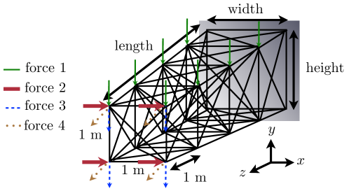
Fig. 2: Clamped–free parameterized truss structure

We set the material properties to those of aluminum, i.e., density $\rho=2700\ \mathrm{kg/m}^{3}$ and elastic modulus $E=62\times 10^{9}$ Pa. The external force is composed of four components:

$$\mathbf{f}({\mu},t)=\sum_{i=1}^{4}{r}_{i}({\mu},t){\mathbf{r}}_{i},$$ (49)

where ${\mathbf{r}}_{i}\in\mathbb{R}^{N}$, $i=1,\ldots,4$ correspond to unit loads uniformly distributed across designated nodes and ${r}_{i}:\mathcal{D}\times\left[0,\mathsf{T}\right]\rightarrow\mathbb{R}$, $i=1,\ldots,4$ denote the component-force magnitudes. Figure  2 depicts the spatial distribution of the forces, which lead to vectors ${\mathbf{r}}_{i}$, $i=1,\ldots,4$ through the finite-element formulation described below. The parameterized, time-dependent magnitudes of these forces are

$${r}_{i}({\mu},t)=\begin{cases}\gamma_{i}\left({\mu}\right)\sin\left(\lambda_{i}({\mu})\left(t-\mathsf{T}/4\right)\right),\quad t\geq\mathsf{T}/4\\ 0,\quad\mbox{otherwise}\end{cases},$$ (50)

where $\gamma_{i}:\mathcal{D}\rightarrow\mathbb{R}$ and $\lambda_{i}:\mathcal{D}\rightarrow\mathbb{R}$, $i=1,\ldots,4$ denote the maximum force magnitudes and force frequencies, respectively. Similarly, the initial condition is composed of four components

$${{\mathbf{q}}(0;{\mu})}=\sum_{i=1}^{4}{s}_{i}({\mu}){\mathbf{s}}_{i},$$ (51)

where ${\mathbf{s}}_{i}$ is the steady-state displacement of the truss subjected to load ${\mathbf{r}}_{i}\gamma_{i}\left(\bar{}{\mu}\right)$ with $\bar{}{\mu}=\left(0,\ldots,0\right)$ denoting the nominal point in parameter space. The equilibrium configuration is simply the undeformed truss represented by ${\mathbf{q}}_{0}\left({\mu}\right)=0$; thus, the configuration space is centered at equilibrium.

The truss is parameterized by 16 parameters ${\mu}\equiv\left({\mu}_{1},\ldots,{\mu}_{16}\right)\in\left[-1,1\right]^{16}$ that affect the geometry, initial condition, and applied force as described in Table 2.

length (m)	bar	width (m)	height (m)	initial condition	external-force	external-force
	cross-sectional			max magnitude (N)	magnitude	frequency
	area ($\mathrm{m}^{2}$)			${s}_{i}$	$\gamma_{i}$	$\lambda_{i}$
$200+50{\mu}_{1}$	$0.0025(1+0.5{\mu}_{2})$	$10(1+{\mu}_{3})$	$10(1+{\mu}_{4})$	$\underline{f}_{i}(1+0.5{\mu}_{i+4})$	$\underline{f}_{i}(1+0.5\mu_{i+8})$	$3\omega_{0}(1+0.5{\mu}_{i+12})$

Table 2: Effect of parameters on truss geometry, initial conditions, and applied forces. Here, $\underline{f}_{i}$, $i=1,\ldots,4$ denote the nominal force magnitudes (to be specified within each experiment) and $\omega_{0}$ denotes the lowest-magnitude eigenvalue of the structure at the nominal point $\bar{}{\mu}$.

The problem is discretized by the finite-element method. The model consists of sixteen three-dimensional bar elements per bay with three degrees of freedom per node; this results in 12 degrees of freedom per bay. We consider a problem with 250 bays, which leads to $N=3\times 10^{3}$ degrees of freedom in the full-order model. The bar elements model geometric nonlinearity, which results in a high-order nonlinearity in the potential-energy $V$.

This discretization leads to a model that corresponds to a Lagrangian dynamical system, with configuration manifold $Q=\mathbb{R}^{N}$, Riemannian metric $g({\mathbf{v}},{\mathbf{w}};{\mu})={\mathbf{v}}^{T}{{\mathbf{M}}\left({\mu}\right)}{\mathbf{w}}$, nonlinear potential-energy function $V$ and dissipation function ${\mathcal{F}\left(\dot{}{\mathbf{q}};{\mu}\right)}\equiv\frac{1}{2}\dot{}{\mathbf{q}}^{T}{{\mathbf{C}}\left({\mu}\right)}\dot{}{\mathbf{q}}$. Here, ${{\mathbf{C}}\left({\mu}\right)}=\alpha{{\mathbf{M}}\left({\mu}\right)}+\beta\nabla_{{\mathbf{q}}{\mathbf{q}}}V(0;{\mu})$ corresponds to Rayleigh damping. Here, $\alpha$ and $\beta$ are chosen such that the damping ratio is a specified value $\zeta$ for the uncoupled ODEs associated with the smallest two eigenvalues of the matrix pencil $\left({\mathbf{M}}(\bar{}{\mu}),\nabla_{{\mathbf{q}}{\mathbf{q}}}V\left(0;\bar{}{\mu}\right)\right)$ [10].

To numerically solve the Lagrangian equations of motion in the time interval $[0,\mathsf{T}]$ with $\mathsf{T}=25$ seconds, we employ the implicit midpoint rule (a symplectic integrator). This ensures that the numerical solution will yield symplectic time-evolution maps in the conservative case. We employ a globalized Newton solver with a More–Thuente linesearch [12] to solve the system of nonlinear algebraic equations arising at each time step. Convergence of the Newton iterations is declared when the residual norm reaches $10^{-6}$ of its value computed using a zero acceleration and the values of the displacement and velocity at the beginning of the timestep. The linear system arising at each Newton iteration is solved directly.

The experiments compare the performance of four reduced-order models: Galerkin projection (Section 5.1), collocation (Section 5.2.1), and gappy POD (Section 5.2.2), and the proposed structure-preserving methods. All reduced-order models (ROMs) employ the same POD reduced basis ${\mathbf{V}}$, which is computed by applying Algorithm 5 with snapshots of the configuration variables and an energy criterion $\eta_{\mathbf{q}}\in\left[0,1\right]$ specified within each experiment. The POD bases ${\mathbf{W}}_{{\boldsymbol{\theta}}}$ employed by the gappy POD approach (see Section 5.2.2) are generated in the same way. In all cases, snapshots are only collected for the first half of the time interval at the training points; as a result, the second half of the time interval can be considered predictive—even for the training set.

Reduced-order models with complexity reduction employ the same sampling matrix ${\mathbf{P}}$, which is generated using GNAT’s greedy sample-mesh algorithm [7]. These models are also implemented using the sample-mesh concept [7]. To solve optimization problems (2), we use the Poblano toolbox for unconstrained optimization [12]. The initial guess for each of these problems is chosen as ${\mathbf{P}}^{T}{\mathbf{P}}{\mathbf{V}}$. In practice, we always found the constraints to be inactive at the unconstrained solution to (12); therefore, this reduces to a linear least-squares problem that we solve directly.

To compare the performance of the reduced-order models, we will consider the response quantity of interest to be the $y$-displacement of the bottom-left node of the end face of the truss in Figure 2; we denote this (parameterized, time-dependent) quantity by $y\in\mathbb{R}$. The reported errors will be a normalized 1-norm (in time) of the error in this quantity:

$$\mathrm{error}=\frac{\sum\limits_{t\in\mathsf{T}_{\mathrm{sample}}({\mu}^{\star})}|y_{\mathrm{ROM}}(t;{\mu}^{\star})-y_{\mathrm{HFM}}(t;{\mu}^{\star})|}{|\mathsf{T}_{\mathrm{sample}}({\mu}^{\star})|\left(\max\limits_{t\in\mathsf{T}_{\mathrm{sample}}({\mu}^{\star})}y_{\mathrm{HFM}}(t;{\mu}^{\star})-\min\limits_{t\in\mathsf{T}_{\mathrm{sample}}({\mu}^{\star})}y_{\mathrm{HFM}}(t;{\mu}^{\star})\right)}.$$ (52)

Here, $y_{\mathrm{ROM}}$ denotes the response computed by a reduced-order model, $y_{\mathrm{HFM}}$ is the high-fidelity ‘truth’ response, and $\mathsf{T}_{\mathrm{sample}}({\mu}^{\star})\subset\left[0,\mathsf{T}\right]$ denotes the time instances selected by the time integrator for online point ${\mu}^{\star}$. In addition to the error in Eq. 52, we will compare the speedup achieved by the reduced-order models, measured as the ratio of the reduced-order-model simulation time to the full-order-model simulation time. All computations are carried out in Matlab on a Mac Pro with 2 $\times$ 2.93 GHz 6-Core Intel Xeon processors and 64 GB of memory.

7.1 Conservative case

We first consider the conservative case characterized by zero damping $\zeta=0$ and no external forces ${\mu}_{i}=-2$ for $i=9,\ldots,16$. This scenario is particularly interesting, as the full-order model corresponds to a conservative Lagrangian dynamical system characterized by energy conservation and symplectic time-evolution maps, and our method can also be interpreted as preserving Hamiltonian structure (see Appendix A). Because we numerically solve the equations of motion using the implicit midpoint rule, which is a symplectic integrator, the numerical solution is also characterized by a sympletic time-evolution map. This will also hold for reduced-order models that preserve Lagrangian structure, i.e., the Galerkin reduced-order model and the two proposed techniques (see Table 1). Note also that the dynamics of undamped, unforced structures are typically quite stiff, which often leaves reduced-order models prone to instabilities. As a result, we are free to vary parameters ${\mu}_{i}$, $i=1,\ldots,8$, which affect only the geometry and initial condition. We set the nominal forces that affect the initial condition to $\underline{f}_{1}=\underline{f}_{2}=2\mathrm{kg}\times 9.81\mathrm{m/s}^{2}$ and $\underline{f}_{3}=\underline{f}_{4}=0.4\mathrm{kg}\times 9.81\mathrm{m/s}^{2}$.

We first perform a timestep-verification study for the nominal point $\bar{}{\mu}$ characterized by $\bar{}{\mu}_{i}=0$, $i=1,\ldots 8$ to ensure we employ an appropriate timestep in the numerical experiments. Results are shown in Figure 3. A timestep size of $\Delta t=0.008$ seconds yields an observed convergence rate in the time-averaged tip displacement of $1.98$, which is close to the asymptotic rate of convergence of the implicit midpoint rule, and an approximated error in the time-averaged tip displacement using Richardson extrapolation of $5.16\times 10^{-7}$. We can therefore declare this to be an appropriate timestep size for the numerical experiments. Further, we note that the average number of Newton iterations per timestep is $3.15$, so the geometric nonlinearity in the potential-energy function is significant.

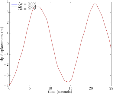
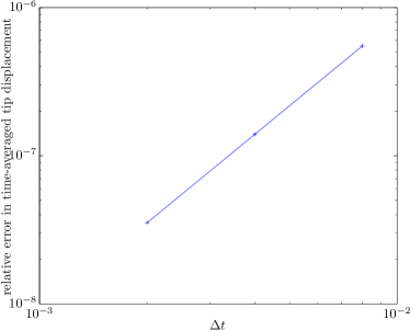
Fig. 3: Conservative case: Timestep verification study at the nominal point. A timestep of $\Delta t=0.008$ seconds gives a convergence rate of $1.98$ and approximate relative error of $5.16\times 10^{-7}$. Note that the three responses in the left figure nearly overlap.

7.1.1 Fixed parameters

We now test the model-reduction techniques in a fixed-parameters scenario. That is, we employ the nominal point in the parameter space for both the training and online points: $\{{\mu}^{i}\}=\bar{}{\mu}$ and ${\mu}^{\star}=\bar{}{\mu}$. Recall that we only collect snapshots for the first half of the time interval, so the second half can be considered a predictive regime. Note that the two proposed structure-preserving methods are the same for this case: they both exactly approximate the reduced mass matrix when the parameters are fixed.

The POD reduced basis ${\mathbf{V}}$ is generated using an energy criterion of $\eta_{\mathbf{q}}=1-10^{-5}$ in Algorithm 5 of Appendix B; this leads to a basis dimension of only $n=11\ll N$. The gappy POD-based reduced-order model employs an energy criterion of $1$ (i.e., no truncation) for its reduced bases ${\mathbf{W}}_{{\boldsymbol{\theta}}}$ (see Section 5.2.2). Figures 4 and 5 report results for the reduced-order models as the number of sample indices varies.

First, note that the Galerkin reduced-order model is accurate (relative error of $5.42\%$); however, it yields a speedup of only 1.69. This is to be expected, as it preserves Lagrangian structure, but has no complexity-reduction mechanism (see Section 5.1.1). In addition, the proposed reduced-order model—which also preserves structure, yet has a complexity-reduction mechanism—yields a stable and accurate response regardless of the number of sample points chosen. For example, $0.4\%$ sampling yields a relative error of 7.3% and a speedup of 207.0. Sampling $2\%$ of the indices yields an error of $0.71\%$ and a speedup of 34.5, and sampling $5\%$ of the indices leads to $0.48\%$ error and a speedup of 15.7. Note that sampling beyond $5\%$ does not improve the method’s accuracy; however, it degrades the speedup, as it requires computing more entries of the vector-valued functions.

The other complexity-reducing reduced-order models (gappy POD and collocation) are always unstable except for collocation in the full-sampling case, when it is equivalent to Galerkin. This clearly highlights the practical benefits of preserving structure in model reduction, as existing structure-destroying complexity-reduction methods failed, even in the relatively simple scenario of fixed parameter values.

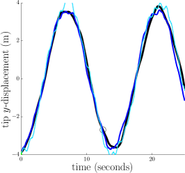
(a) 0.4% sampling

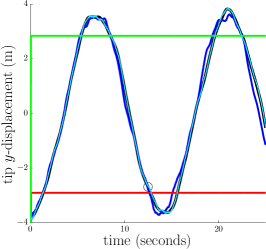
(b) 2% sampling

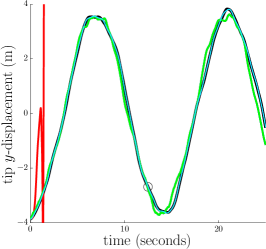
(c) 100% sampling

Fig. 4: Conservative, fixed-parameters case: reduced-order model responses as a function of sampling percentage $m/N\times 100\%$. Legend: full-order model (black), Galerkin ROM (dark blue), structure-preserving ROM (light blue), gappy POD ROM (red), collocation ROM (green), end of training time interval (black circle).

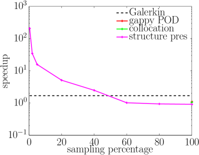
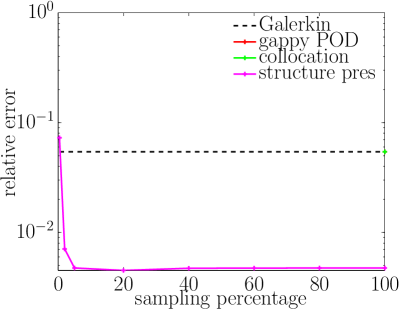
Fig. 5: Conservative, fixed-parameters case: reduced-order model performance as a function of sampling percentage $m/N\times 100\%$. Missing data points for gappy POD and collocation ROMs indicate unstable responses.

7.1.2 Varying parameters

We now consider a fully predictive scenario with ${\mu}^{\star}\not\in\{{\mu}^{i}\}$. We use $p=6$ training points and determine $\{{\mu}^{i}\}$ using Latin hypercube sampling. The online points are subsequently chosen randomly in the parameter space. Figure 6 depicts the tip displacement for the training points. Note that the responses are significantly different from one another. The two proposed structure-preserving reduced-order models will now be different from one another, as the parameters are varying, which means that the parameterized mass matrix will be approximated differently by the two techniques (see Table 1).

Fig. 6: Conservative, varying-parameters case: tip displacement for the training set $\{{\mu}^{i}\}$.

The reduced-order models employ a POD reduced basis with a truncation energy criterion of $\eta_{\mathbf{q}}=1-10^{-6}$, which yields a basis dimension of $n=147\ll N$. Again, the gappy POD-based reduced-order model employs a truncation criterion of $\eta_{\boldsymbol{\theta}}=1$ for its reduced bases. Figure 7 reports the tip displacements generated by the reduced-order models for the three randomly chosen online points, and Figure 8 reports the speedup and errors achieved by the reduced-order models as a function of the number of sample indices.

Again, note that the Galerkin reduced-order model is stable and accurate, as it generates relative errors of 18.7%, 14.5%, and 9.16% at the three online points, respectively. However, it yields discouraging speedups of 0.81 (i.e., the simulation was slower than for the full-order model), 1.61, and 1.32 at these points. The proposed structure-preserving methods are always stable and quite accurate. They yield nearly the same performance, although method two (which employs the matrix gappy POD approximation) generates lower errors for online points with $4.9\%$ sampling. From Figure 7, note that the high-frequency oscillations that characterize the proposed methods’ responses are smoothed out when the sampling percentage reaches 20%. In particular, proposed method 2 generates speedups of 15.9, 28.5, and 26.2 and relative errors of 11.6%, 13.0%, and 11.6% for 4.9% sampling. For 20% sampling, the method generates speedups of 4.84, 9.82, and 7.72, and relative errors of 1.51%, 5.83%, and 1.09%.

In this example, the gappy POD reduced-order model is unstable for all sampling percentages, and the collocation reduced-order model is only stable for 100% sampling (at which point it is mathematically equivalent to the Galerkin reduced-order model). This is not surprising, as these methods do not preserve problem structure, nor do they guarantee energy conservation. This poor performance can be attributed to the stiff dynamics that characterize the considered conservative Lagrangian dynamical system, which lead to instabilities for both reduced-order models.

This example strongly showcases the practical importance of preserving Lagrangian structure: the proposed structure-preserving reduced-order models are the only models that yield both fast and accurate results.

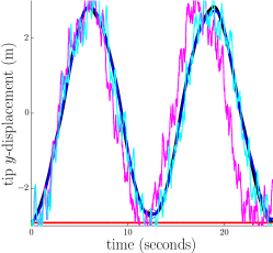
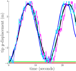
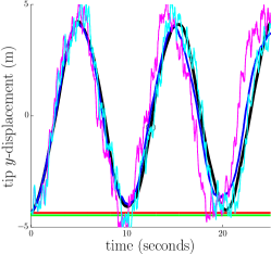
(a) $4.9\%$ sampling

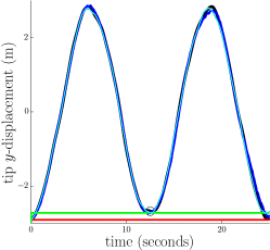
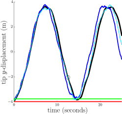
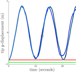
(b) $20\%$ sampling

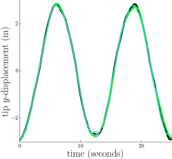
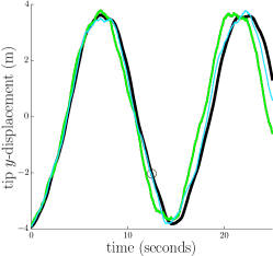
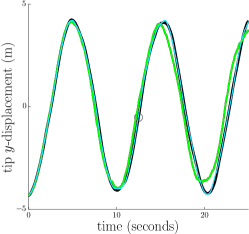
(c) $100\%$ sampling

Fig. 7: Conservative, varying-parameters case: reduced-order model responses as a function of sampling percentage $m/N\times 100\%$ for three randomly chosen online points. Legend: full-order model (black), Galerkin ROM (dark blue), structure-preserving ROM method 1 (magenta), structure-preserving ROM method 2 (light blue), gappy POD ROM (red), collocation ROM (green), end of training time interval (black circle).

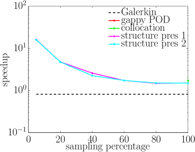
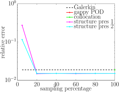
(a) online point 1

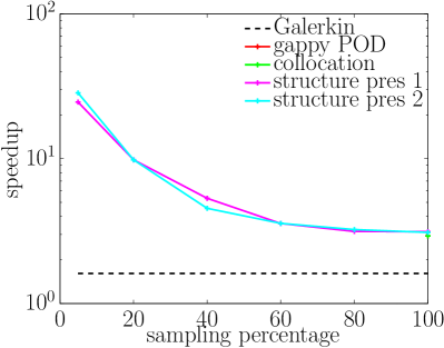
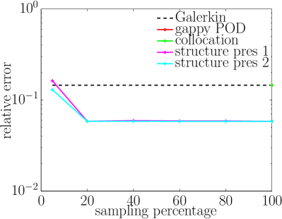
(b) online point 2

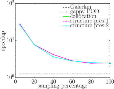
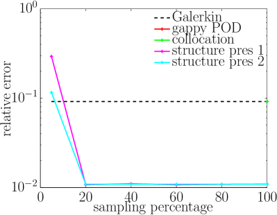
(c) online point 3

Fig. 8: Conservative, varying-parameters case: reduced-order model performance as a function of sampling percentage $m/N\times 100\%$.

7.2 Non-conservative case

We now consider the non-conservative case in which the non-conservative dissipative and external forces are nonzero. That is, we set $\zeta=\mathrm{sin}(5^{\circ})$ and all parameters ${\mu}_{i}$, $i=1,\ldots,16$ are free to vary. We again set the nominal forces to $\bar{f}_{1}=\bar{f}_{2}=2\mathrm{kg}\times 9.81\mathrm{m/s}^{2}$ and $\bar{f}_{3}=\bar{f}_{4}=0.4\mathrm{kg}\times 9.81\mathrm{m/s}^{2}$.

As before, we perform a timestep-verification study for the nominal point $\bar{}{\mu}$ characterized by $\bar{}{\mu}_{i}=0$, $i=1,\ldots 16$ to discover an appropriate timestep. A timestep size of $\Delta t=0.1$ seconds leads to an approximated error using Richardson extrapolation of $1.07\times 10^{-4}$. We can therefore declare this to be an appropriate timestep size for the numerical experiments. Further, we note that the average number of Newton iterations per timestep is $2.56$, so the nonlinearity remains significant.

7.2.1 Fixed parameters

We again test the different methods in the fixed-parameters case where $\{{\mu}^{i}\}=\bar{}{\mu}$ and ${\mu}^{\star}=\bar{}{\mu}$. As above, we only collect snapshots for the first half of the time interval, and the proposed structure-preserving methods yield the same results.

The POD reduced basis ${\mathbf{V}}$ is generated using an energy criterion of $\eta_{\mathbf{q}}=1-10^{-5}$, which leads to a basis dimension of $n=6\ll N$. The gappy POD-based reduced-order model employs an energy criterion of $1$ for its reduced bases ${\mathbf{W}}_{{\boldsymbol{\theta}}}$. Figures 9 and 10 report results for the reduced-order models as the number of sample indices varies.

Again, the Galerkin reduced-order model is accurate, with a relative error of 1.57%, but produces a speedup of only 1.33. The proposed structure-preserving method is always stable as expected. Its performance is dependent upon the sampling percentage, with (arguably) the best performance achieved for 2% sampling (6.28% error and 36.5 speedup). For 0.2% sampling, the method produces 16.1% error and a speedup of 251; 20% sampling leads to 5.39% error and a speedup of 4.6.

The gappy POD reduced-order model is unstable for 0.2%, 2%, and 5% sampling, but stabilizes at 20%; compared to the conservative case, this stability likely results from less stiff dynamics due to the presence of damping. This yields its best performance of 1.53% error, but only a 4.1 speedup. The collocation reduced-order model is stable only for full sampling, when it is equivalent to Galerkin.

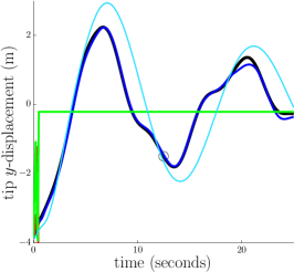
(a) 0.2% sampling

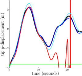
(b) 5% sampling

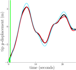
(c) 20% sampling

Fig. 9: Non-conservative, fixed-parameters case: reduced-order model responses as a function of sampling percentage $m/N\times 100\%$. Legend: full-order model (black), Galerkin ROM (dark blue), structure-preserving ROM (light blue), gappy POD ROM (red), collocation ROM (green), end of training time interval (black circle).

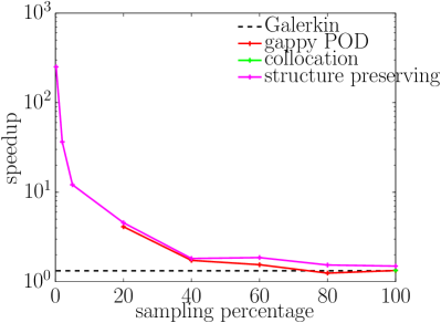
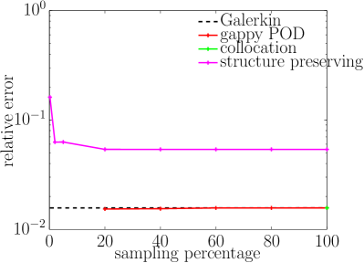
Fig. 10: Non-conservative, fixed-parameters case: reduced-order model performance as a function of sampling percentage $m/N\times 100\%$. Missing data points for gappy POD and collocation ROMs indicate unstable responses.

7.2.2 Varying parameters

We now consider the parameter-varying case where ${\mu}^{\star}\not\in\{{\mu}^{i}\}$. We again employ $p=6$ training points and determine $\{{\mu}^{i}\}$ using Latin hypercube sampling. We choose the online points randomly in the parameter space. Figure 11(a) shows the tip displacement for the training points; clearly, the responses are significantly different from one another.

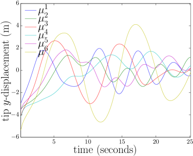
(a) Section 7.2 experiments

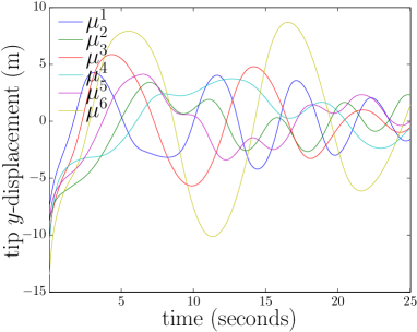
(b) Section 7.3 experiments (higher nonlinearity)

Fig. 11: Non-conservative, parameter-varying case: tip displacement for the training set $\{{\mu}^{i}\}$ for two sets of experiments.

Because we are in a fully predictive scenario, the two proposed structure-preserving reduced-order models again yield different results. All reduced-order models employ an energy criterion of $\eta_{\mathbf{q}}=1-10^{-5}$, which leads to a basis dimension of $n=12$. We employ $\eta_{\boldsymbol{\theta}}=1$ for the gappy POD reduced-order model.

Figures 12 and 13 report the results for this predictive study at the online points. At all three points, Galerkin is accurate (relative errors of 9.8%, 7.5%, and 13.5%), but does not yield significant speedups (speedups of 1.2, 1.4, and 1.1). As is apparent from the plots, the two proposed structure-preserving methods yield nearly the same performance. At 0.4% sampling, method 1 produces relative errors of 11.0%, 2.82%, and 10.3% and speedups of 73.3, 96.3, and 82.3. At 2% sampling, method 1 yields relative errors of 10.9%, 4.38%, and 7.97% and speedups of 19.2, 21.6, and 16.8.

In this example, gappy POD does not stabilize until 40% sampling, at which point the speedup is less than 1. Thus, gappy POD does not yield performance improvement for this problem. Collocation stabilizes at 80% sampling, and also fails to generate any performance improvement.

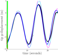
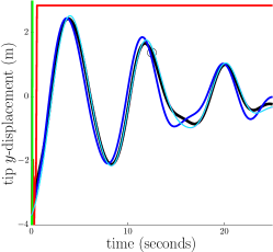
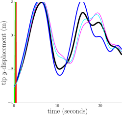
(a) predictions at three randomly chosen online points, $0.4\%$ sampling

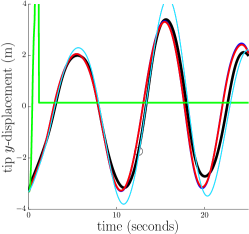
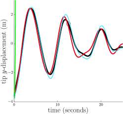
(b) predictions at three randomly chosen online points, $40\%$ sampling

(c) predictions at three randomly chosen online points, $80\%$ sampling

Fig. 12: Non-conservative, parameter-varying case: reduced-order model responses as a function of sampling percentage $m/N\times 100\%$. Legend: full-order model (black), Galerkin ROM (dark blue), structure-preserving ROM method 1 (magenta), structure-preserving ROM method 2 (light blue), gappy POD ROM (red), collocation ROM (green), end of training time interval (black circle).

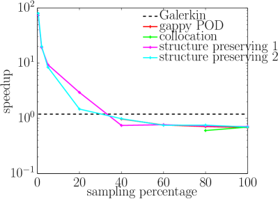
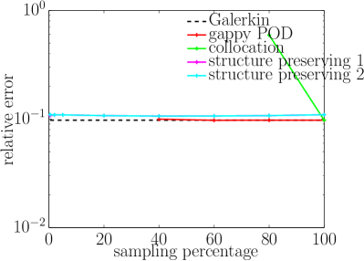
(a) online point 1

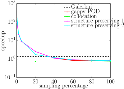
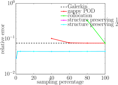
(b) online point 2

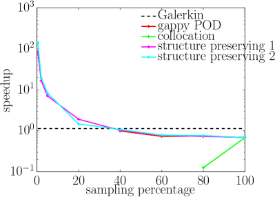
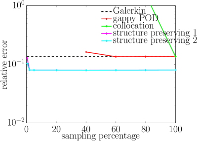
(c) online point 3

Fig. 13: Non-conservative, parameter-varying case: reduced-order model performance as a function of sampling percentage $m/N\times 100\%$.

7.3 Effect of nonlinearity

We now aim to characterize the dependence of problem nonlinearity on the proposed methods’ performances. Recall from Section 3 that the potential-energy approximation is computed by matching the gradient of the potential energy to first order about the equilibrium configuration ${\mathbf{q}}_{0}\left({\mu}^{\star}\right)$. In the presence of stronger nonlinearity, we expect the configuration to deviate further from equilibrium, which should degrade the accuracy of the approximation.

To numerically assess the effect of nonlinearity, we repeat the experiments from Section 7.2.2 using the same training and online points, but we increase the nominal forces by a factor of 2.5 to $\underline{f}_{1}=\underline{f}_{2}=5\mathrm{kg}\times 9.81\mathrm{m/s}^{2}$ and $\underline{f}_{3}=\underline{f}_{4}=1\mathrm{kg}\times 9.81\mathrm{m/s}^{2}$. We first perform a timestep-verification study for the nominal point $\bar{}{\mu}$. As expected, a smaller timestep size of $\Delta t=0.025$ seconds is required, as it corresponds to an approximated error using Richardson extrapolation of $3.62\times 10^{-4}$.

Figure 11(b) displays the tip displacement for the training points. Note that the responses are similar to those for the previous study (see Figure 11(a)), but have larger magnitudes and therefore imply a stronger geometric nonlinearity. The reduced-order models employ a POD reduced basis of dimension $n=14$, which was obtained by an energy criterion of $\eta_{\mathbf{q}}=1-10^{-5}$; gappy POD uses $\eta_{\boldsymbol{\theta}}=1$ for its nonlinear-function bases.

Figures 14 and 15 report the reduced-order models’ performances for this problem. As in the previous case, Galerkin is accurate (relative errors of 8.3%, 3.0%, and 10.0% at the online points), but does not generate significant speedups (1.67, 1.71, and 1.0). The proposed structure-preserving techniques again yield very similar results to each other; however, the errors are significantly larger than in the the experiments from Section 7.2.2 characterized by a less severe nonlinearity. For 0.5% sampling, proposed method 1 yields relative errors of 21.3%, 11.1%, and 15.9% at the online points and speedups of 116.4, 160, and 98.9. Thus, increasing the nonlinearity in the problem does have a deleterious effect on the methods’ performances.

However, it is important to note that other complexity-reducing reduced-order models fail to generate significant performance improvement on this more highly nonlinear problem. In particular collocation is always unstable for a sampling percentage less than 60%, and gappy POD is always unstable when the percentage is less than 80%. As a result, the best speedup obtained by either of the methods is only 2.77 (collocation for 60% sampling for online point 2).

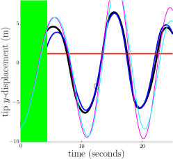
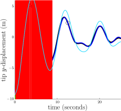
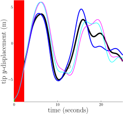
(a) predictions at three randomly chosen online points, $0.5\%$ sampling

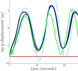
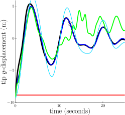
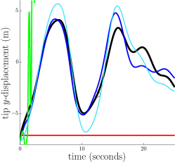
(b) predictions at three randomly chosen online points, $60\%$ sampling

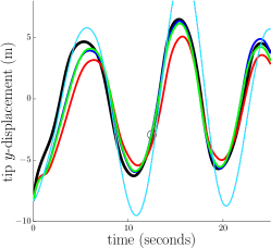
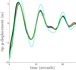
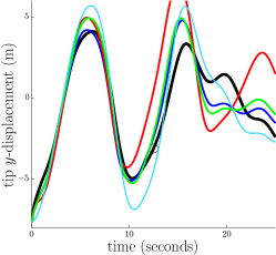
(c) predictions at three randomly chosen online points, $80\%$ sampling

Fig. 14: Non-conservative, highly nonlinear parameter-varying case: reduced-order model responses as a function of sampling percentage $m/N\times 100\%$. Legend: full-order model (black), Galerkin ROM (dark blue), structure-preserving ROM method 1 (magenta), structure-preserving ROM method 2 (light blue), gappy POD ROM (red), collocation ROM (green), end of training time interval (black circle).

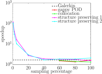
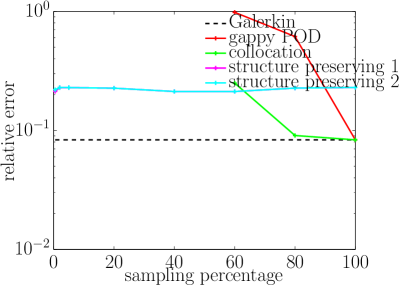
(a) online point 1

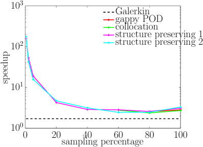
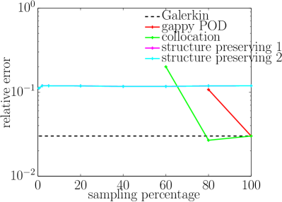
(b) online point 2

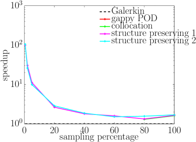
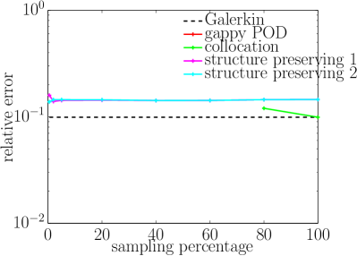
(c) online point 3

Fig. 15: Non-conservative, highly nonlinear parameter-varying case: reduced-order model performance as a function of sampling percentage $m/N\times 100\%$.

8 Conclusions

This paper has presented an efficient structure-preserving model-reduction strategy applicable to simple mechanical systems. The methodology directly approximates the quantities that define the problem’s Lagrangian structure and subsequently derives the equations of motion, while ensuring low online computational cost. The method is distinct from typical model-reduction methods for nonlinear ODEs; these methods are typically based on collocation and DEIM/gappy POD techniques that approximate the equations of motion and destroy Lagrangian structure. At the core of the methodology are the reduced-basis sparsification (RBS) and matrix gappy POD techniques for approximating parameterized reduced matrices while preserving symmetry and positive definiteness; we also employed the former method to preserve potential-energy structure.

Numerical experiments on a geometrically nonlinear parameterized truss structure highlight the method’s benefits: preserving Lagrangian structure ensured the method always generated stable responses that were often very accurate. Other model-reduction techniques were often unstable; achieving stability usually required too many sample indices to lead to significant performance gains for those methods. The experiments also showed that both RBS and matrix gappy POD led to nearly the same performance across a range of experiments.

Future work includes devising a method to improve the method’s robustness in the presence of strong nonlinearity (e.g., by non-local approximation of the potential-energy function), applying the method to a truly large-scale problem, devising a technique-specific method for choosing the sample indices, and deriving error bounds and error estimates that rigorously assess the accuracy of the method’s predictions. Finally, the RBS and matrix gappy POD methods are relevant to a wider class of problems than model reduction for Lagrangian systems; future work will investigate to their applicability to other scenarios.

Appendix A Hamiltonian dynamics

When the Hamiltonian formulation of classical mechanics is taken, the proposed structure-preserving reduced-order models also preserve problem structure. For simplicity, we consider conservative systems with no dissipation or applied external forces. The Hamiltonian ingredients for conservative simple mechanical systems are then the same as those for Lagrangian dynamical systems as described in Section 1:

• A differentiable configuration manifold $Q$, which we set to $Q=\mathbb{R}^{N}$.

• A parameterized Riemannian metric $g({\mathbf{v}},{\mathbf{w}};{\mu})$, which we set to $g({\mathbf{v}},{\mathbf{w}};{\mu})={\mathbf{v}}^{T}{{\mathbf{M}}\left({\mu}\right)}{\mathbf{w}}$, where ${{\mathbf{M}}\left({\mu}\right)}$ denotes the $N\times N$ parameterized symmetric positive-definite mass matrix.

• A parameterized potential-energy function $V:Q\times\mathcal{D}\rightarrow\mathbb{R}$.

Again, the kinetic energy can be expressed as $T(\dot{}{\mathbf{q}};{\mu})=\frac{1}{2}g(\dot{}{\mathbf{q}},\dot{}{\mathbf{q}};{\mu})=\frac{1}{2}\dot{}{\mathbf{q}}^{T}{{\mathbf{M}}\left({\mu}\right)}\dot{}{\mathbf{q}}$, and the Lagrangian becomes $L({\mathbf{q}},\dot{}{\mathbf{q}};{\mu})=\frac{1}{2}\dot{}{\mathbf{q}}^{T}{{\mathbf{M}}\left({\mu}\right)}\dot{}{\mathbf{q}}-V({\mathbf{q}};{\mu})$.

The conjugate momenta ${\mathbf{p}}:\left[0,\mathsf{T}\right]\times\mathcal{D}\rightarrow\mathbb{R}^{N}$ can then be derived as

$${\mathbf{p}}(t;{\mu}) =\frac{\partial L}{\partial\dot{}{\mathbf{q}}}\left(t;{\mu}\right)$$ (53)

$$={{\mathbf{M}}\left({\mu}\right)}\dot{}{\mathbf{q}}(t;{\mu}).$$ (54)

In terms of the conjugate momenta, the kinetic energy then becomes $T_{\mathbf{q}}({\mathbf{p}};{\mu})={\mathbf{p}}^{T}{{\mathbf{M}}\left({\mu}\right)}^{-1}{\mathbf{p}}$. By definition, the Hamiltonian $H:\mathbb{R}^{N}\times\mathbb{R}^{N}\times\mathcal{D}\rightarrow\mathbb{R}$ is the Legendre transformation of the Lagrangian function:

$$H({\mathbf{p}},{\mathbf{q}};{\mu}) =\dot{}{\mathbf{q}}^{T}{\mathbf{p}}-L({\mathbf{q}},\dot{}{\mathbf{q}},t)$$ (55)

$$=\frac{1}{2}{\mathbf{p}}^{T}{{\mathbf{M}}\left({\mu}\right)}^{-1}{\mathbf{p}}+V({\mathbf{q}};{\mu}).$$ (56)

Equivalently, it is the total energy, or sum of the kinetic and potential energies for classical mechanical systems. The equations of motion can then be obtained by applying Hamilton’s equations of motion

$$\dot{}{\mathbf{q}} =\frac{\partial H}{\partial{\mathbf{p}}}$$ (57)

$$\dot{}{\mathbf{p}} =-\frac{\partial H}{\partial{\mathbf{q}}},$$ (58)

which are equivalent to

$$\dot{}{\mathbf{q}}={{\mathbf{M}}\left({\mu}\right)}{\mathbf{q}}$$ (59)

$${{\mathbf{M}}\left({\mu}\right)}\ddot{}{\mathbf{q}}+\nabla_{\mathbf{q}}V({\mathbf{q}};{\mu})=0$$ (60)

from the definition of the Hamiltonian and conjugate momenta. Note that these are equivalent to the equations of motion for a simple mechanical system (26) in the conservative case derived using the Lagrangian formalism.

A.1 Galerkin reduced-order model

To construct the structure-preserving Galerkin reduced-order model for the Hamiltonian formalism, we follow this same recipe, but with the reduced ingredients defined previously. First, we define the reduced configuration space $Q_{r}\in\mathbb{R}^{n}$ with $\mathsf{Q}_{r}\equiv\{\bar{}{\mathbf{q}}({\mu})+{\mathbf{V}}{{\mathbf{q}}_{r}}\ |\ {{\mathbf{q}}_{r}}\in Q_{r}\}$, and subsequently the reduced Lagrangian from Eqs. (31)–(32)

$$L_{r}({{\mathbf{q}}_{r}},\dot{}{{\mathbf{q}}_{r}};{\mu}) \equiv L(\bar{}{\mathbf{q}}({\mu})+{\mathbf{V}}{{\mathbf{q}}_{r}},{\mathbf{V}}\dot{}{{\mathbf{q}}_{r}};{\mu})$$ (61)

$$=\frac{1}{2}\dot{}{{\mathbf{q}}_{r}}^{T}{\mathbf{V}}^{T}{{\mathbf{M}}\left({\mu}\right)}{\mathbf{V}}\dot{}{{\mathbf{q}}_{r}}-V(\bar{}{\mathbf{q}}({\mu})+{\mathbf{V}}{{\mathbf{q}}_{r}};{\mu}).$$ (62)

Then, the reduced conjugate momenta ${\mathbf{p}_{r}}:\left[0,\mathsf{T}\right]\times\mathcal{D}\rightarrow\mathbb{R}^{n}$ can be computed as

$${\mathbf{p}_{r}}(t;{\mu}) =\frac{\partial L_{r}}{\partial\dot{}{{\mathbf{q}}_{r}}}\left(t;{\mu}\right)$$ (63)

$$={\mathbf{V}}^{T}{{\mathbf{M}}\left({\mu}\right)}{\mathbf{V}}\dot{}{{\mathbf{q}}_{r}}(t;{\mu}),$$ (64)

and the reduced Hamiltonian is, by definition,

$$H_{r}({\mathbf{p}_{r}},{{\mathbf{q}}_{r}};{\mu}) =\dot{}{{\mathbf{q}}_{r}}^{T}{\mathbf{p}_{r}}-L({{\mathbf{q}}_{r}},\dot{}{{\mathbf{q}}_{r}},t)$$ (65)

$$=\frac{1}{2}{\mathbf{p}_{r}}^{T}\left({\mathbf{V}}^{T}{{\mathbf{M}}\left({\mu}\right)}{\mathbf{V}}\right)^{-1}{\mathbf{p}_{r}}+V(\bar{}{\mathbf{q}}({\mu})+{\mathbf{V}}{{\mathbf{q}}_{r}};{\mu}).$$ (66)

Applying Hamilton’s equations of motion then yields

$$\dot{}{{\mathbf{q}}_{r}} =\frac{\partial H_{r}}{\partial{\mathbf{p}_{r}}}$$ (67)

$$\dot{}{\mathbf{p}_{r}} =-\frac{\partial H_{r}}{\partial{{\mathbf{q}}_{r}}},$$ (68)

or equivalently

$$\dot{}{{\mathbf{q}}_{r}}={\mathbf{V}}^{T}{{\mathbf{M}}\left({\mu}\right)}{\mathbf{V}}{{\mathbf{q}}_{r}}$$ (69)

$${\mathbf{V}}^{T}{{\mathbf{M}}\left({\mu}\right)}{\mathbf{V}}\ddot{}{{\mathbf{q}}_{r}}+{\mathbf{V}}^{T}\nabla_{\mathbf{q}}V(\bar{}{\mathbf{q}}({\mu})+{\mathbf{V}}{{\mathbf{q}}_{r}};{\mu})=0$$ (70)

Again, these are equivalent to the Galerkin reduced-order equations of motion (37) obtained from the Lagrangian perspective in the absence of non-conservative forces. Clearly, this formulation for a reduced-order model preserves Hamiltonian structure, as the equations of motion are consistent with the Hamiltonian formalism.

A.2 Proposed structure-preserving methods

The proposed methods preserve Hamiltonian structure. The derivation follows that of the Galerkin reduced-order model in the previous section, but with the reduced Lagrangian replaced by the approximated reduced Lagrangian from Eq. (62):

$$\tilde{L}_{r}({{\mathbf{q}}_{r}},\dot{}{{\mathbf{q}}_{r}};{\mu}) =\frac{1}{2}\tilde{g}_{r}(\dot{}{{\mathbf{q}}_{r}},\dot{}{{\mathbf{q}}_{r}};{\mu})-\tilde{}V_{r}({{\mathbf{q}}_{r}};{\mu})$$ (71)

$$=\frac{1}{2}\dot{}{{\mathbf{q}}_{r}}^{T}\tilde{}{\mathbf{M}}\left({\mu}\right)\dot{}{{\mathbf{q}}_{r}}-\tilde{}V_{r}({{\mathbf{q}}_{r}};{\mu}),$$ (72)

where $\tilde{}{\mathbf{M}}\left({\mu}\right)$ is an $n\times n$ symmetric positive definite matrix generated by one of the methods presented in Section 2, and $\tilde{}V_{r}({{\mathbf{q}}_{r}};{\mu})$ is an approximated potential approximated according to the method outlined in Section 3.

The approximated reduced conjugate momenta are then

$$\tilde{}{\mathbf{p}_{r}}(t;{\mu}) =\frac{\partial\tilde{L}_{r}}{\partial\dot{}{{\mathbf{q}}_{r}}}\left(t;{\mu}\right)$$ (73)

$$=\tilde{}{\mathbf{M}}\left({\mu}\right)\dot{}{{\mathbf{q}}_{r}}(t;{\mu}),$$ (74)

and the approximated reduced Hamilton is

$$\tilde{H}_{r}(\tilde{}{\mathbf{p}_{r}},{{\mathbf{q}}_{r}};{\mu}) =\dot{}{{\mathbf{q}}_{r}}^{T}\tilde{}{\mathbf{p}_{r}}-L({{\mathbf{q}}_{r}},\dot{}{{\mathbf{q}}_{r}},t)$$ (75)

$$=\frac{1}{2}\tilde{}{\mathbf{p}_{r}}^{T}\tilde{}{\mathbf{M}}\left({\mu}\right)^{-1}\tilde{}{\mathbf{p}_{r}}+\tilde{}V_{r}({{\mathbf{q}}_{r}};{\mu}).$$ (76)

Applying Hamilton’s equations yields the following equations of motion

$$\dot{}{{\mathbf{q}}_{r}}=\tilde{}{\mathbf{M}}\left({\mu}\right){{\mathbf{q}}_{r}}$$ (77)

$$\tilde{}{\mathbf{M}}\left({\mu}\right)\ddot{}{{\mathbf{q}}_{r}}+\nabla_{{\mathbf{q}}_{r}}\tilde{}V_{r}({{\mathbf{q}}_{r}};{\mu})=0,$$ (78)

which are computationally inexpensive to solve, and also retain Hamiltonian structure, as they are consistent with the Hamiltonian formalism. Note that again these are equivalent to the equations of motion obtained with the proposed strategy in the Lagrangian case with non-conservative forces set to zero.

Appendix B Proper orthogonal decomposition

Algorithm 5 describes the method for computing a proper orthogonal decomposition (POD) basis given a set of snapshots. The method amounts to computing the singular value decomposition of the snapshot matrix; the left singular vectors define the POD basis.

Procedure 5 Proper-orthogonal-decomposition basis computation (normalized snapshots)

0:  Set of snapshots $\mathcal{X}\equiv\{\mathbf{x}_{i}\}_{i=1}^{n_{\mathbf{x}}}\subset\mathbb{R}^{N}$, energy criterion $\eta\in[0,1]$

0:  ${\mathbf{W}}\left(\mathcal{X},\eta\right)$

1:   Compute the thin singular value decomposition $\mathbf{X}=\mathbf{U}\Sigma\mathbf{V}^{T}$, where $\mathbf{X}\equiv\left[\mathbf{x}_{1}/\|\mathbf{x}_{1}\|\ \cdots\ \mathbf{x}_{n_{\mathbf{x}}}/\|\mathbf{x}_{n_{\mathbf{x}}}\|\right]$.

2:  Choose dimension of truncated basis $n=n_{e}(\eta)$, where

$$n_{e}(\eta) \equiv\min_{i\in\mathcal{V}(\eta)}i$$ (79)

$$\mathcal{V}(\eta) \equiv\{n\in\{1,\ldots,{n_{\mathbf{x}}}\}\ |\ \sum_{i=1}^{n}\sigma_{i}^{2}/\sum_{j=1}^{{n_{\mathbf{x}}}}\sigma_{j}^{2}\geq\eta\},$$ (80)

and $\Sigma\equiv\mathrm{diag}\left(\sigma_{i}\right)$ with $\sigma_{1}\geq\cdots\geq\sigma_{n_{\mathbf{x}}}\geq 0$.

3:  ${\mathbf{W}}\left(\mathcal{X},\eta\right)=\left[\mathbf{u}^{1}\ \cdots\ \mathbf{u}^{n}\right]$, where $\mathbf{U}\equiv\left[\mathbf{u}^{1}\ \cdots\ \mathbf{u}^{{n_{\mathbf{x}}}}\right]$.

Appendix C Solving the matrix gappy POD optimization problem

This approach reformulates the constraints of problem (11) in terms of eigenvalues of the reduced matrix. That is, problem (11) is reformulated as

$$\begin{split}\underset{x\equiv\left(x_{1},\ldots,x_{n_{\mathbf{A}}}\right)}{\mathrm{minimize}}\quad&\|{{\mathbf{P}}^{T}}{\mathbf{A}\left({\mu}\right)}{\mathbf{P}}-\sum\limits_{k=1}^{n_{\mathbf{A}}}{{\mathbf{P}}^{T}}{\underline{\mathbf{A}}}_{k}{\mathbf{P}}x_{k}\|_{F}^{2}\\ \mathrm{subject\ to}\quad&{\tilde{\lambda}}_{j}(x)\geq\epsilon>0,\quad j=1,\ldots,n.\\ \end{split}$$ (81)

Here, ${\tilde{\lambda}}_{j}(x)$, $j=1,\ldots,n$ are the eigenvalues of the low-dimensional matrix $\sum\limits_{i=1}^{n_{\mathbf{A}}}{\mathbf{V}}^{T}{\underline{\mathbf{A}}}_{i}{\mathbf{V}}x_{i}$ and $\epsilon$ denotes a numerical threshold for defining a full-rank matrix. This problem can be numerically solved, e.g., using a gradient-based algorithm.

The gradient of the quadratic objective function is obvious. The gradient of the constraint can be derived by assuming distinct eigenvalues:

$$\frac{\partial{\tilde{\lambda}}_{j}}{\partial x_{i}} ={\tilde{\mathbf{y}}}_{j}^{T}\frac{\partial\left(\sum\limits_{k=1}^{n_{\mathbf{A}}}{\mathbf{V}}^{T}{\underline{\mathbf{A}}}_{k}{\mathbf{V}}x_{k}\right)}{\partial x_{i}}{\tilde{\mathbf{y}}}_{j}$$ (82)

$$={\tilde{\mathbf{y}}}_{j}^{T}\left({\mathbf{V}}^{T}{\underline{\mathbf{A}}}_{i}{\mathbf{V}}\right){\tilde{\mathbf{y}}}_{j}.$$ (83)

Here, ${\tilde{\mathbf{y}}}_{j}$ is the eigenvector associated with eigenvalue ${\tilde{\lambda}}_{j}$. This indicates that computing the gradient $\frac{\partial{\tilde{\lambda}}_{j}}{\partial x_{i}}$ is inexpensive and requires the following steps:

1. Compute the eigenvector ${\tilde{\mathbf{y}}}_{j}\in\mathbb{R}^{n}$ of the matrix $\sum\limits_{k=1}^{n_{\mathbf{A}}}{\mathbf{V}}^{T}{\underline{\mathbf{A}}}_{k}{\mathbf{V}}x_{k}$.

2. Compute the low-dimensional matrix–vector product ${\mathbf{w}}=\left({\mathbf{V}}^{T}{\underline{\mathbf{A}}}_{i}{\mathbf{V}}\right){\tilde{\mathbf{y}}}_{j}$.

3. Compute the low-dimensional vector–vector product ${\tilde{\mathbf{y}}}_{j}^{T}{\mathbf{w}}$.

We propose using the unconstrained solution to problem (81) as the initial guess. In practice, this solution is often feasible, so it is typically unnecessary to handle the constraints directly. In the rare cases where it is necessary to deal with multiple equal eigenvalues—or a number of nearby eigenvalues—the methods presented by Andrew and Tan [3] can be used to produce a numerically stable gradient of the constraint; this was not required in the numerical experiments reported in Section 7.

Appendix D Proofs

D.1 Proof of Theorem 2.2

The proof relies on a generalization of the well known Cauchy interlacing thereom. To prove this generalization, we use a theorem (Theorem 4.3.10) from Ref. [16] that we restate below.

Theorem D.6.

Let two sequences of interlacing real numbers be given by $(\lambda^{(r)}_{i})_{i=1}^{n}$ and $(\lambda^{(s)}_{i})_{i=1}^{m}$ as described by inequality (5) when $m=n+1$. Define $\boldsymbol{\Lambda}^{(r)}=\mathop{\operator@font diag}\nolimits(\lambda^{(r)}_{i})$ and $\boldsymbol{\Lambda}^{(s)}=\mathop{\operator@font diag}\nolimits(\lambda^{(s)}_{i})$. Then, there exists a real number $\alpha\in\mathbb{R}$ and a vector $\mathbf{y}\in\mathbb{R}^{n}$ such that $\boldsymbol{\Lambda}^{(s)}$ are the eigenvalues of the real symmetric matrix

$$\hat{\mathbf{B}}^{(\mathrm{bordered})}\equiv\left(\begin{matrix}\boldsymbol{\Lambda}^{(r)}&\mathbf{y}\cr\mathbf{y}^{T}&\alpha\end{matrix}\right).$$

The following corollary is a direct consequence of the above theorem.

Corollary D.7.

Given $\hat{\mathbf{B}}^{(s)}\in\mathrm{SPD}\left(m\right)$ and $\hat{\mathbf{B}}^{(r)}\in\mathrm{SPD}\left(m-1\right)$, where $\mathrm{SPD}\left(k\right)$ denotes the set of $k\times k$ symmetric positive-definite matrices, whose eigenvalues interlace, then

$$\exists~{}\mathbf{U}_{m}~{}\mbox{such that }\mathbf{U}_{m}^{T}\hat{\mathbf{B}}^{(s)}\mathbf{U}_{m}=\hat{\mathbf{B}}^{(r)}~{}~{}~{}~{}\mbox{with}~{}~{}~{}~{}\mathbf{U}_{m}^{T}\mathbf{U}_{m}=I.$$ (84)

Proof D.8.

Using the above theorem, a matrix $\hat{\mathbf{B}}^{(\mathrm{bordered})}\in\mathrm{SPD}\left(m\right)$ exists that shares the same eigenvalues with $\hat{\mathbf{B}}^{(s)}$. Let $\mathbf{Q}^{(\mathrm{bordered})}$, $\mathbf{Q}^{(s)}$, and $\mathbf{Q}^{(r)}$ be the (square, orthogonal) matrices of eigenvectors for $\hat{\mathbf{B}}^{(\mathrm{bordered})}$, $\hat{\mathbf{B}}^{(s)}$, and $\hat{\mathbf{B}}^{(r)}$, respectively. Then,

$$\left(\mathbf{Q}^{(\mathrm{bordered})}\right)^{T}\hat{\mathbf{B}}^{(\mathrm{bordered})}\mathbf{Q}^{(\mathrm{bordered})}=\boldsymbol{\Lambda}^{(s)}=\mathbf{Q}^{(s)}\hat{\mathbf{B}}^{(s)}(\mathbf{Q}^{(s)})^{T},$$

which implies that

$$\hat{\mathbf{B}}^{(\mathrm{bordered})}=\mathbf{Q}^{(\mathrm{bordered})}(\mathbf{Q}^{(s)})^{T}\hat{\mathbf{B}}^{(s)}\mathbf{Q}^{(s)}(\mathbf{Q}^{(\mathrm{bordered})})^{T}.$$

From the definition of $\hat{\mathbf{B}}^{(\mathrm{bordered})}$ it also follows that

$$[\mathbf{I}~{}~{}~{}\mathbf{0}]\hat{\mathbf{B}}^{(\mathrm{bordered})}[\mathbf{I}~{}~{}~{}\mathbf{0}]^{T}=\boldsymbol{\Lambda}^{(r)},$$

where $I$ is the $(m-1)\times(m-1)$ identity matrix and $\mathbf{0}$ is the zero column vector of length $m-1$, and thus

$$\hat{\mathbf{B}}^{(r)}=\mathbf{Q}^{(r)}\boldsymbol{\Lambda}^{(r)}(\mathbf{Q}^{(r)})^{T}=\mathbf{Q}^{(r)}\left[[\mathbf{I}~{}~{}~{}\mathbf{0}]\hat{\mathbf{B}}^{(\mathrm{bordered})}[\mathbf{I}~{}~{}~{}\mathbf{0}]^{T}\right](\mathbf{Q}^{(r)})^{T}.$$ (85)

Combining the above, we can write

$$\hat{\mathbf{B}}^{(r)}=\mathbf{Q}^{(r)}[\mathbf{I}~{}~{}~{}\mathbf{0}]\mathbf{Q}^{(\mathrm{bordered})}(\mathbf{Q}^{(s)})^{T}\hat{\mathbf{B}}^{(s)}\mathbf{Q}^{(s)}(\mathbf{Q}^{(\mathrm{bordered})})^{T}[\mathbf{I}~{}~{}~{}\mathbf{0}]^{T}(\mathbf{Q}^{(r)})^{T}$$

and so (84) is satisfied taking $\mathbf{U}_{m}=\left[\mathbf{Q}^{(r)}[\mathbf{I}~{}~{}~{}\mathbf{0}]\mathbf{Q}^{(\mathrm{bordered})}(\mathbf{Q}^{(s)})^{T}\right]^{T}$.

The generalization of the Cauchy interlacing thereom now follows.

Theorem D.9.

Given two matrices $\hat{\mathbf{B}}^{(s)}\in\mathrm{SPD}\left(m\right)$ and $\hat{\mathbf{B}}^{(r)}\in\mathrm{SPD}\left(n\right)$ (with $m\geq n$), then

$$\exists~{}\mathbf{U}~{}~{}\mbox{such that}~{}~{}~{}\mathbf{U}^{T}\hat{\mathbf{B}}^{(s)}\mathbf{U}=\hat{\mathbf{B}}^{(r)}~{}~{}~{}~{}\mbox{with}~{}~{}~{}~{}\mathbf{U}^{T}\mathbf{U}=\mathbf{I}$$ (86)

if and only if the eigenvalues ${\lambda}_{i}^{(r)}$, $i=1,\ldots,n$ interlace the eigenvalues ${\lambda}_{i}^{(s)}$, $i=1,\ldots,m$ defined as

$$\hat{\mathbf{B}}^{(r)}\hat{\mathbf{x}}_{i}^{(r)} ={\lambda}_{i}^{(r)}\hat{\mathbf{x}}_{i}^{(r)},\quad i=1,\ldots,n$$ (87)

$$\hat{\mathbf{B}}^{(s)}\hat{\mathbf{x}}_{i}^{(s)} ={\lambda}_{i}^{(s)}\hat{\mathbf{x}}_{i}^{(s)},\quad i=1,\ldots,m.$$ (88)

The definition of interlacing is given by inequality (5).

Proof D.10.

It is well known that if $\hat{\mathbf{B}}^{(s)}\in\mathrm{SPD}\left(m\right)$ is given along with an orthogonal $m\times n$ matrix $\mathbf{U}$ (with $m\geq n$), then the eigenvalues of $\mathbf{U}^{T}\hat{\mathbf{B}}^{(s)}\mathbf{U}$ must interlace those of $\hat{\mathbf{B}}^{(s)}$. This is referred to as the Cauchy interlacing theorem (e.g., see [20]).

The converse of the Cauchy interlacing theorem is less widely known. The case $m=n$ follows trivially using an eigenvalue decomposition. The case $m=n+1$ corresponds to the above corollary. The proof is completed by generalizing the corollary to the $m>n+1$ case. This follows from an inductive argument where one considers a projection that reduces the matrix dimension of $\hat{\mathbf{B}}^{(s)}$ by one. According to the above corollary, we have a great deal of flexibility in choosing this lower dimensional matrix if its eigenvalues interlace those of the higher dimension matrix. We then choose a lower dimensional matrix whose eigenvalues not only interlace those of $\hat{\mathbf{B}}^{(s)}$ but whose eigenvalues are also interlaced by those of $\hat{\mathbf{B}}^{(r)}$. That is,

$$\lambda_{i}^{(s)}\leq\mu_{i}\leq\lambda_{i+1}^{(s)}~{}~{}~{}\mbox{and}~{}~{}~{}\mu_{i}\leq\lambda_{i}^{(r)}\leq\mu_{i+m-n-1},$$

where $\mu_{i}$ denotes the $i$th smallest eigenvalue of the intermediate matrix. Rewriting this we obtain the following intervals for the eigenvalues $\mu_{i}$:

$$\mu_{i}\geq\left\{\begin{array}[]{cc}\max(\lambda_{i}^{(s)},\lambda_{i-m+n+1}^{(r)})&i\geq m-n\\ \lambda_{i}^{(s)}&i<m-n\end{array}\right.$$

and

$$\mu_{i}\leq\left\{\begin{array}[]{cc}\min(\lambda_{i+1}^{(s)},\lambda_{i}^{(r)})&i\leq n\\ \lambda_{i+1}^{(s)}&i>n\end{array}\right..$$

Using the interlacing property for $\hat{\mathbf{B}}^{(s)}$ and $\hat{\mathbf{B}}^{(r)}$, one can verify that the intervals for the $\mu_{i}$ are nonempty. That is, $\lambda_{i+1}^{(s)}\geq\lambda_{i}^{(s)}$ and for those $i$ such that $\lambda_{i-m+n+1}^{(r)}$ is defined, we have $\lambda_{i+1}^{(s)}\geq\lambda_{i-m+n+1}^{(r)},~{}\lambda_{i}^{(r)}\geq\lambda_{i}^{(s)},~{}\mbox{and}~{}\lambda_{i}^{(r)}\geq\lambda_{i-m+n+1}^{(r)}$ Thus, there exists an orthogonal matrix $\mathbf{U}_{m}$ such that the $(m\hskip-2.168pt-\hskip-2.168pt1)\times(m\hskip-2.168pt-\hskip-2.168pt1)$ matrix $\mathbf{U}_{m}^{T}\hat{\mathbf{B}}^{(s)}\mathbf{U}_{m}$ has eigenvalues that are interlaced by those of $\hat{\mathbf{B}}^{(r)}$. We repeat this procedure each time reducing the matrix dimension by one until the final reduction where we take the lower dimension matrix to be equal to $\hat{\mathbf{B}}^{(r)}$. This implies that there exists a set of projection matrices such that $\mathbf{U}^{T}\hat{\mathbf{B}}^{(s)}\mathbf{U}$ is equal to $\hat{\mathbf{B}}^{(r)}$ where $\mathbf{U}=\mathbf{U}_{m}\mathbf{U}_{m-1}...\mathbf{U}_{n+1}$.

Equipped with the generalized Cauchy interlacing theorem, we now prove the exactness condition for the ${\mathbf{A}\left({\mu}\right)}$ term which is restated in slightly simplified notation.

Theorem D.11.

Let ${\mathbf{A}\left({\mu}\right)}$ have the form

$${\mathbf{A}\left({\mu}\right)}={{{h}_{1}}\left({\mu}\right)}~{}{\mathbf{A}_{1}}+{{{h}_{2}}\left({\mu}\right)}~{}{\mathbf{A}_{2}}$$ (89)

where ${\mathbf{A}_{1}}\in\mathrm{SPD}\left(N\right)$, ${\mathbf{A}_{2}}\in\mathrm{SPD}\left(N\right)$, and ${{h}_{1}},{{h}_{2}}:\mathcal{D}\rightarrow\mathbb{R}$. Then,

$$\exists~{}\underline{{{\mathbf{U}}_{\mathbf{A}}}}~{}~{}\mbox{such that}~{}~{}~{}\underline{{{\mathbf{U}}_{\mathbf{A}}}}^{T}\hskip 1.8063pt{{\mathbf{P}}^{T}}\hskip 1.8063pt{\mathbf{A}\left({\mu}\right)}\hskip 1.8063pt{\mathbf{P}}\hskip 1.8063pt\underline{{{\mathbf{U}}_{\mathbf{A}}}}={\mathbf{V}}^{T}\hskip 1.8063pt{\mathbf{A}\left({\mu}\right)}\hskip 1.8063pt{\mathbf{V}},~{}~{}~{}~{}\forall{\mu}\in\mathcal{D}$$ (90)

if and only if the eigenvalues of the general matrix pencil

$$\mathbf{B}^{(r)}\mathbf{x}_{i}^{(r)}=\lambda_{i}^{(r)}\mathbf{D}^{(r)}\mathbf{x}_{i}^{(r)},\quad i=1,\ldots,n$$ (91)

interlace the eigenvalues of

$$\mathbf{B}^{(s)}\mathbf{x}_{i}^{(s)}=\lambda_{i}^{(s)}\mathbf{D}^{(s)}\mathbf{x}_{i}^{(s)},\quad i=1,\ldots,m$$ (92)

where

$$\begin{array}[]{lllllll}\mathbf{D}^{(r)}&=&\left[{\mathbf{V}}^{T}{\mathbf{A}_{1}}{\mathbf{V}}\right],&&\mathbf{D}^{(s)}&=&\left[{{\mathbf{P}}^{T}}{\mathbf{A}_{1}}{\mathbf{P}}\right],\\[10.0pt] \mathbf{B}^{(r)}&=&\left[{\mathbf{V}}^{T}{\mathbf{A}_{2}}{\mathbf{V}}\right],&~{}~{}\mbox{and}{}{}&\mathbf{B}^{(s)}&=&\left[{{\mathbf{P}}^{T}}{\mathbf{A}_{2}}{\mathbf{P}}\right].\end{array}$$

The definition of interlacing is given by

$$\lambda^{(s)}_{i}\leq\lambda^{(r)}_{i}\leq\lambda^{(s)}_{i+m-n}~{}~{}~{}for~{}i=1,...,n$$ (93)

where the eigenvalues are indexed in order of increasing magnitude.

Proof D.12.

Clearly (90) can only hold for any ${\mu}\in\mathcal{D}$ and any functions ${{{h}_{1}}\left({\mu}\right)}$ and ${{{h}_{2}}\left({\mu}\right)}$ if and only if

$$\underline{{{\mathbf{U}}_{\mathbf{A}}}}^{T}\mathbf{D}^{(s)}\underline{{{\mathbf{U}}_{\mathbf{A}}}}=\mathbf{D}^{(r)}~{}~{}\mbox{and}~{}~{}\underline{{{\mathbf{U}}_{\mathbf{A}}}}^{T}\mathbf{B}^{(s)}\underline{{{\mathbf{U}}_{\mathbf{A}}}}=\mathbf{B}^{(r)}.$$ (94)

Using a carefully chosen linear transformation, it follows that proving the theorem is equivalent to proving the following:

$$\exists~{}\mathbf{U}~{}~{}\mbox{such that}~{}~{}~{}\mathbf{U}^{T}\hat{\mathbf{B}}^{(s)}\mathbf{U}=\hat{\mathbf{B}}^{(r)}~{}~{}~{}~{}\mbox{with}~{}~{}~{}~{}\mathbf{U}^{T}\mathbf{U}=\mathbf{I}$$ (95)

if and only if the eigenvalues $\lambda_{i}^{(r)}$ interlace the eigenvalues of $\lambda_{i}^{(s)}$, where the eigenvalues previously defined in Eqs. (91)–(92) also satisfy

$$\begin{split}\hat{\mathbf{B}}^{(r)}\hat{\mathbf{x}}^{(r)}&={\lambda}^{(r)}\hat{\mathbf{x}}^{(r)}\\ \hat{\mathbf{B}}^{(s)}\hat{\mathbf{x}}^{(s)}&={\lambda}^{(s)}\hat{\mathbf{x}}^{(s)}.\end{split}$$ (96)

The linear transformation relies on Cholesky factorizations given by $\mathbf{D}^{(s)}=\mathbf{L}^{(s)}(\mathbf{L}^{(s)})^{T}$ and $\mathbf{D}^{(r)}=\mathbf{L}^{(r)}(\mathbf{L}^{(r)})^{T}$. These factors lead to the following definitions

$$\begin{array}[]{llllll}\hat{\mathbf{B}}^{(s)}&=&(\mathbf{L}^{(s)})^{-1}\mathbf{B}^{(s)}(\mathbf{L}^{(s)})^{-T},&\hat{\mathbf{x}}^{(s)}&=&(\mathbf{L}^{(s)})^{T}\mathbf{x}^{(s)},\\[5.0pt] \hat{\mathbf{B}}^{(r)}&=&(\mathbf{L}^{(r)})^{-1}\mathbf{B}^{(r)}(\mathbf{L}^{(r)})^{-T},&\hat{\mathbf{x}}^{(r)}&=&(\mathbf{L}^{(r)})^{T}\mathbf{x}^{(r)},~{}~{}\mbox{and}\\[5.0pt] \mathbf{U}&=&(\mathbf{L}^{(s)})^{T}\underline{{{\mathbf{U}}_{\mathbf{A}}}}(\mathbf{L}^{(r)})^{-T},\end{array}$$

which can be used in Eqs. (91), (92) and (94) to obtain Eqs. (95) and (96). The proof is completed by recognizing that Eqs. (95) and (96) correspond to the generalized Cauchy interlacing thereorm.

D.2 Proof of Theorem 2.3

Proof D.13.

If condition 2 holds, then the unconstrained solution to problem (11) is

$$\xi_{\mathbf{A}}\left({\mu}^{\star}\right)=\left(\bar{}{\mathbf{P}}^{T}{{\mathbf{W}}_{\mathbf{a}}}\right)^{+}\bar{}{\mathbf{P}}^{T}v\left({\mathbf{A}\left({\mu}^{\star}\right)}\right).$$ (97)

If condition 1 holds, then the vectorized matrix can be expressed as

$$v\left({\mathbf{A}\left({\mu}^{\star}\right)}\right)={{\mathbf{W}}_{\mathbf{a}}}\mathbf{z}\left({\mu}^{\star}\right),$$ (98)

or equivalently

$${\mathbf{A}\left({\mu}^{\star}\right)}=\sum_{i=1}^{n_{\mathbf{A}}}z^{i}\left({\mu}^{\star}\right){{\underline{\mathbf{A}}}_{i}},$$ (99)

where $\mathbf{z}\equiv\left(z^{1},\ldots,z^{{n_{\mathbf{A}}}}\right)$. Substituting Eq. (98) into Eq. (97) gives $\xi_{\mathbf{A}}\left({\mu}^{\star}\right)=\mathbf{z}\left({\mu}^{\star}\right)$ and so Eq. (6) yields

$$\tilde{\mathbf{A}}\left({\mu}^{\star}\right) =\sum\limits_{i=1}^{n_{\mathbf{A}}}z^{i}\left({\mu}^{\star}\right){\mathbf{V}}^{T}{\underline{\mathbf{A}}}_{i}{\mathbf{V}}.$$ (100)

Comparing Eqs. (100) and (99) gives the exactness result: $\tilde{\mathbf{A}}\left({\mu}^{\star}\right)={\mathbf{V}}^{T}{\mathbf{A}\left({\mu}^{\star}\right)}{\mathbf{V}}^{T}$.

D.3 Proof of Lemma 1

Proof D.14.

The equation $\widetilde{{{{\mathbf{U}}_{V}}}}^{T}\widetilde{{{{\mathbf{U}}_{V}}}}=I$ simply states that the $m$ columns of $\widetilde{{{{\mathbf{U}}_{V}}}}$ are orthogonal and so any orthogonal matrix $\widetilde{{{{\mathbf{U}}_{V}}}}$ satisfies the first part of (20). Thus, solvability amounts to finding an orthogonal matrix $\widetilde{{{{\mathbf{U}}_{V}}}}$ such that $\tilde{{\mathbf{V}}}^{T}\tilde{\mathbf{c}}=\widetilde{{{{\mathbf{U}}_{V}}}}^{T}{{\mathbf{P}}^{T}}\tilde{\mathbf{c}}$. For a solution to exist, however, it is obviously necessary that $||\tilde{{\mathbf{V}}}^{T}\tilde{\mathbf{c}}||_{2}=||\widetilde{{{{\mathbf{U}}_{V}}}}^{T}{{\mathbf{P}}^{T}}\tilde{\mathbf{c}}||_{2}$. If the vector ${{\mathbf{P}}^{T}}\tilde{\mathbf{c}}$ lies within the span of the basis defined by the columns of $\widetilde{{{{\mathbf{U}}_{V}}}}^{T}$, then $\widetilde{{{{\mathbf{U}}_{V}}}}^{T}{{\mathbf{P}}^{T}}\tilde{\mathbf{c}}$ preserves its 2-norm and so $||\widetilde{{{{\mathbf{U}}_{V}}}}^{T}{{\mathbf{P}}^{T}}\tilde{\mathbf{c}}||_{2}=||{{\mathbf{P}}^{T}}\tilde{\mathbf{c}}||_{2}$. That is, application of $\widetilde{{{{\mathbf{U}}_{V}}}}^{T}$ corresponds to a rotation of ${{\mathbf{P}}^{T}}\tilde{\mathbf{c}}$ about the origin and so length is preserved. If instead the vector ${{\mathbf{P}}^{T}}\tilde{\mathbf{c}}$ lies only partially within the span of the orthogonal basis, then $||\widetilde{{{{\mathbf{U}}_{V}}}}^{T}{{\mathbf{P}}^{T}}\tilde{\mathbf{c}}||_{2}<||{{\mathbf{P}}^{T}}\tilde{\mathbf{c}}||_{2}$. That is, application of $\widetilde{{{{\mathbf{U}}_{V}}}}^{T}$ corresponds to a rotation of the component of ${{\mathbf{P}}^{T}}\tilde{\mathbf{c}}$ lying within the span of the orthogonal basis. This implies that a necessary condition for a solution to (20) is that

$$||\tilde{{\mathbf{V}}}^{T}\tilde{\mathbf{c}}||_{2}\leq||{{\mathbf{P}}^{T}}\tilde{\mathbf{c}}||_{2}.$$ (101)

Case 1: $m=n$
${{\mathbf{P}}^{T}}\tilde{\mathbf{c}}$ must lie within the range of $\widetilde{{{{\mathbf{U}}_{V}}}}$ (as it is a full rank square matrix) and so it is necessary to have equality in (101) when $m=n$. One possible $\widetilde{{{{\mathbf{U}}_{V}}}}$ in this case is obtained by first defining a $\mathbf{Q}_{1}\in\mathbb{R}^{n\times n}$ and a $\mathbf{Q}_{2}\in\mathbb{R}^{n\times n}$ such that the first row of $\mathbf{Q}_{1}$ is $\alpha_{1}\tilde{\mathbf{c}}^{T}\tilde{{\mathbf{V}}}$ with $\alpha_{1}=1/\|\tilde{\mathbf{c}}^{T}\tilde{{\mathbf{V}}}\|_{2}$. Likewise, the first row of $\mathbf{Q}_{2}$ is taken as $\alpha_{1}\tilde{\mathbf{c}}^{T}{\mathbf{P}}$; note that $\alpha_{1}$ also normalizes this row because we assume $\|\tilde{{\mathbf{V}}}^{T}\tilde{\mathbf{c}}\|_{2}=\|{{\mathbf{P}}^{T}}\tilde{\mathbf{c}}\|_{2}$. All remaining rows are chosen so that both $\mathbf{Q}_{1}$ and $\mathbf{Q}_{2}$ are orthogonal matrices. This gives

$$\mathbf{Q}_{1}\tilde{}{\mathbf{V}}^{T}\tilde{\mathbf{c}}=||\tilde{}{\mathbf{V}}^{T}\tilde{\mathbf{c}}||_{2}\mathbf{e}_{1}=||{{\mathbf{P}}^{T}}\tilde{\mathbf{c}}||_{2}\mathbf{e}_{1}=\mathbf{Q}_{2}{{\mathbf{P}}^{T}}\tilde{\mathbf{c}},$$

where $\mathbf{e}_{1}$ is the first canonical unit vector of length $n$ (first element is one and all other $n-1$ components are zero). A suitable $\widetilde{{{{\mathbf{U}}_{V}}}}$ that solves (20) is then given by $\widetilde{{{{\mathbf{U}}_{V}}}}^{T}=\mathbf{Q}_{1}^{T}\mathbf{Q}_{2}$. Thus, equality in (101) is also sufficient when $m=n$. Case 2: $m>n$
The matrix $\widetilde{{{{\mathbf{U}}_{V}}}}$ is now rectangular. One possible $\widetilde{{{{\mathbf{U}}_{V}}}}$ is obtained by defining $\mathbf{Q}_{1}$ as before while instead defining an $m\times m$ orthogonal matrix $\mathbf{Q}_{\mathrm{full}}$ with the first row again set to $\alpha_{2}\tilde{\mathbf{c}}^{T}{\mathbf{P}}$ with $\alpha_{2}=1/\|{{\mathbf{P}}^{T}}\tilde{}\mathbf{c}\|_{2}$. This gives

$$\mathbf{Q}_{1}\tilde{}{\mathbf{V}}^{T}\tilde{\mathbf{c}}=||\tilde{}{\mathbf{V}}^{T}\tilde{\mathbf{c}}||_{2}\mathbf{e}_{1}~{}~{}\mbox{and}~{}~{}\mathbf{Q}_{\mathrm{full}}{{\mathbf{P}}^{T}}\tilde{\mathbf{c}}=||{{\mathbf{P}}^{T}}\tilde{\mathbf{c}}||_{2}\tilde{e}_{1}$$

where $\tilde{e}_{1}\in\mathbb{R}^{m\times 1}$ is the first canonical unit vector of length $m$. If $||{{\mathbf{P}}^{T}}\tilde{\mathbf{c}}||_{2}=||\tilde{}{\mathbf{V}}^{T}\tilde{\mathbf{c}}||_{2}$, then a suitable $\tilde{{\mathbf{V}}}$ solving (20) is given by taking $\mathbf{Q}_{2}$ to be the first $n$ rows of $\mathbf{Q}_{\mathrm{full}}$ (as $\mathbf{Q}_{1}\tilde{}{\mathbf{V}}^{T}\tilde{\mathbf{c}}=\mathbf{Q}_{2}{{\mathbf{P}}^{T}}\tilde{\mathbf{c}}$) and taking $\widetilde{{{{\mathbf{U}}_{V}}}}^{T}=\mathbf{Q}_{1}^{T}\mathbf{Q}_{2}$. If $||{{\mathbf{P}}^{T}}\tilde{\mathbf{c}}||_{2}>||\tilde{}{\mathbf{V}}^{T}\tilde{\mathbf{c}}||_{2}$, then we define a vector $y$ as an arbitrary linear combination of the last $m-n$ rows of $\mathbf{Q}_{\mathrm{full}}$ such that $y$ has unit norm. The first row of $\mathbf{Q}_{2}$ is then taken as

$$(\mathbf{Q}_{2})_{1}=\alpha_{3}\frac{{{\mathbf{P}}^{T}}\tilde{\mathbf{c}}}{||{{\mathbf{P}}^{T}}\tilde{\mathbf{c}}||_{2}}+\sqrt{1-\alpha_{3}^{2}}~{}y,$$

where $(\mathbf{Q})_{k}$ denotes the $k$th row of a matrix $\mathbf{Q}$ and $\alpha_{3}=||\tilde{{\mathbf{V}}}^{T}\tilde{\mathbf{c}}||_{2}/||{{\mathbf{P}}^{T}}\tilde{\mathbf{c}}||_{2}$. The remaining rows of $\mathbf{Q}_{2}$ are simply $(\mathbf{Q}_{\mathrm{full}})_{k}$ for $k=2,\ldots,n$. It is easy to verify that $\mathbf{Q}_{2}$ is again orthogonal and that $\mathbf{Q}_{2}{{\mathbf{P}}^{T}}\tilde{\mathbf{c}}=||\tilde{}{\mathbf{V}}^{T}\tilde{\mathbf{c}}||_{2}\mathbf{e}_{1}$. Thus, $\mathbf{Q}_{2}{{\mathbf{P}}^{T}}\tilde{\mathbf{c}}=||\tilde{}{\mathbf{V}}^{T}\tilde{\mathbf{c}}||_{2}\mathbf{e}_{1}$ and $\widetilde{{{{\mathbf{U}}_{V}}}}^{T}=\mathbf{Q}_{1}^{T}\mathbf{Q}_{2}$ is a possible solution implying that $||{{\mathbf{P}}^{T}}\tilde{\mathbf{c}}||_{2}\geq||\tilde{}{\mathbf{V}}^{T}\tilde{\mathbf{c}}||_{2}$ is a necessary and sufficient condition when $m>n$.

References

- [1] S. Adhikari, Damping models for structural vibration, PhD thesis, Cambridge University, September 2000.
- [2] S.S. An, T. Kim, and D.L. James, Optimizing cubature for efficient integration of subspace deformations, ACM Transactions on Graphics (TOG), 27 (2008), p. 165.
- [3] Alan L. Andrew and Roger C. E. Tan, Computation of derivatives of repeated eigenvalues and the corresponding eigenvectors of symmetric matrix pencils, SIAM J. Matrix Anal. Appl., 20 (1998), pp. 78–100.
- [4] P. Astrid, S. Weiland, K. Willcox, and T. Backx, Missing point estimation in models described by proper orthogonal decomposition, IEEE Transactions on Automatic Control, 53 (2008), pp. 2237–2251.
- [5] C. Beattie and S. Gugercin, Structure-preserving model reduction for nonlinear port-hamiltonian systems, in Decision and Control and European Control Conference (CDC-ECC), 2011 50th IEEE Conference on, IEEE, 2011, pp. 6564–6569.
- [6] K. Carlberg, C. Bou-Mosleh, and C. Farhat, Efficient non-linear model reduction via a least-squares Petrov–Galerkin projection and compressive tensor approximations, International Journal for Numerical Methods in Engineering, 86 (2011), pp. 155–181.
- [7] K. Carlberg, C. Farhat, J. Cortial, and D. Amsallem, The GNAT method for nonlinear model reduction: effective implementation and application to computational fluid dynamics and turbulent flows, Journal of Computational Physics, 242 (2013), pp. 623–647.
- [8] K. Carlberg, R. Tuminaro, and P. Boggs, Efficient structure-preserving model reduction for nonlinear mechanical systems with application to structural dynamics, in AIAA Paper 2012-1969, 53rd AIAA/ASME/ASCE/AHS/ASC Structures, Structural Dynamics and Materials Conference, Honolulu, Hawaii, April 23–26 2012.
- [9] S. Chaturantabut and D. C. Sorensen, Nonlinear model reduction via discrete empirical interpolation, SIAM Journal on Scientific Computing, 32 (2010), pp. 2737–2764.
- [10] I. Chowdhury and S.P. Dasgupta, Computation of Rayleigh damping coefficients for large systems, The Electronic Journal of Geotechnical Engineering, 8 (2003).
- [11] M. Drohmann, B. Haasdonk, and M. Ohlberger, Reduced basis approximation for nonlinear parametrized evolution equations based on empirical operator interpolation, SIAM Journal on Scientific Computing, 34 (2012), pp. A937–A969.
- [12] D.M. Dunlavy, T.G. Kolda, and E. Acar, Poblano v 1.0: A Matlab toolbox for gradient-based optimization, Sandia National Laboratories, Albuquerque, NM and Livermore, CA, Tech. Rep. SAND, 1422 (2010).
- [13] R. Everson and L. Sirovich, Karhunen–Loève procedure for gappy data, Journal of the Optical Society of America A, 12 (1995), pp. 1657–1664.
- [14] D. Galbally, K. Fidkowski, K. Willcox, and O. Ghattas, Non-linear model reduction for uncertainty quantification in large-scale inverse problems, International Journal for Numerical Methods in Engineering, 81 (2009), pp. 1581–1608.
- [15] E. Hairer, C. Lubich, and G. Wanner, Geometric numerical integration: structure-preserving algorithms for ordinary differential equations, vol. 31, Springer Verlag, 2006.
- [16] R.A. Horn and C.R. Johnson, Matrix Analysis, Cambridge University Press, 1990.
- [17] K. Ito and SS Ravindran, A reduced basis method for control problems governed by PDEs, Control and estimation of distributed parameter systems, (1998), pp. 153–168.
- [18] S. Lall, P. Krysl, and J.E. Marsden, Structure-preserving model reduction for mechanical systems, Physica D: Nonlinear Phenomena, 184 (2003), pp. 304–318.
- [19] J.E. Marsden and M. West, Discrete mechanics and variational integrators, Acta Numerica, 10 (2001), p. 514.
- [20] Beresford N Parlett, The symmetric eigenvalue problem, vol. 7, SIAM, 1980.
- [21] C. Prud’homme, D. V. Rovas, K. Veroy, L. Machiels, Y. Maday, A. T. Patera, and G. Turinici, Reliable real-time solution of parameterized partial differential equations: Reduced-basis output bound methods, Journal of Fluids Engineering, 124 (2002), pp. 70–80.
- [22] C. Prud’Homme, Dimitrios V Rovas, Karen Veroy, Luc Machiels, Yvon Maday, Anthony T Patera, Gabriel Turinici, et al., Reliable real-time solution of parametrized partial differential equations: Reduced-basis output bound methods, Journal of Fluids Engineering, 124 (2001), pp. 70–80.
- [23] D. Ryckelynck, A priori hyperreduction method: an adaptive approach, Journal of Computational Physics, 202 (2005), pp. 346–366.
- [24] T. Tonn, Reduced-Basis Method (RBM) for Non-Affine Elliptic Parameterized PDEs, PhD thesis, Ulm University, December 2011.
- [25] B. Vandereycken, Low-rank matrix completion by Riemannian optimization, SIAM Journal on Optimization, 23 (2013), pp. 1214—1236.
- [26] D. Wirtz, D. C. Sorensen, and B. Haasdonk, A-posteriori error estimation for DEIM reduced nonlinear dynamical systems, Preprint Series, Stuttgart Research Centre for Simulation Technology, (2012).