Implicit dose-response curves

Abstract.

We develop tools from computational algebraic geometry for the study of steady state features of autonomous polynomial dynamical systems via elimination of variables. In particular, we obtain nontrivial bounds for the steady state concentration of a given species in biochemical reaction networks with mass-action kinetics. This species is understood as the output of the network and we thus bound the maximal response of the system. The improved bounds give smaller starting boxes to launch numerical methods. We apply our results to the sequential enzymatic network studied in (Markevich et al., 2004) to find nontrivial upper bounds for the different substrate concentrations at steady state.

Our approach does not require any simulation, analytical expression to describe the output in terms of the input, or the absence of multistationarity. Instead, we show how to extract information from effectively computable implicit dose-response curves, with the use of resultants and discriminants. We moreover illustrate in the application to an enzymatic network, the relation between the exact implicit dose-response curve we obtain symbolically and the standard hysteresis diagram provided by a numerical ode solver.

The setting and tools we propose could yield many other results adapted to any autonomous polynomial dynamical system, beyond those where it is possible to get explicit expressions.

Keywords: chemical reaction networks, steady states, bounds, resultants, maximal response

1. Introduction

Consider an autonomous polynomial dynamical system

(1) $$\dfrac{d}{dt}x(t)=f(x(t))$$

where $x=(x_{1},\dots,x_{s})$ and $t$ are real variables, and each coordinate $f_{i}$ is a polynomial in $x_{1},\dots,x_{s}$ with real coefficients. The steady states of (1) are thus the real zeros of the algebraic variety defined by $f_{1}(x)=\dots=f_{s}(x)=0$. An important example of these systems are chemical reaction networks with mass-action kinetics, which have been extensively studied on a mathematical basis since the foundational work by Feinberg (Feinberg, 1979), Horn and Jackson (Horn and Jackson, 1972) and Vol^′pert (Vol^′pert and Hudjaev, 1985). In this case, $x_{1},x_{2},\ldots,x_{s}$ represent species concentrations, considered as functions of time $t$ and the meaningful steady states are those with nonnegative coordinates. We will mainly use the terminology of chemical reaction networks throughout and consider nonnegative $x_{i}$.

Any linear relation (with real coefficients) among the polynomials $f_{1},\dots,f_{s}$ defines a conservation relation of the form

(2) $$L(x)\,=\,\ell(x)-b\,=\,0,$$

where $\ell$ is a homogeneous linear form in the variables $x_{1},\dots,x_{s}$ and the constant $b=\ell(x^{*})\in\mathbb{R}$ is determined by the initial values $x^{*}=x(0)$ of the system.

Definition 1.1.

We say that $b>0$ is a trivial upper bound for the $i$th species if there exists a conservation relation $a_{1}x_{1}+a_{2}x_{2}+\dots+x_{i}+\dots+a_{s}x_{s}-b=0$ with all $a_{j}\geq 0$.

In the particular important case of conservative networks, there are trivial upper bounds for the concentrations of all the species. Note that in the conditions of Definition 1.1, $b$ is an upper bound for the concentration of $x_{i}$ along the whole trajectory in $\mathbb{R}_{\geq 0}^{s}$. Our main goal is to improve these bounds for steady state concentrations of specific species of the system (that we will call output). It is important to notice that, in general, there is no analytical expression to describe these concentrations and there could be multistationarity, which makes finding these bounds a difficult task.

In the special bacterial EnvZ/OmpR osmolarity regulator, algebraic methods are used in Karp et al. (2012) to detect the existence of robust upper bounds at steady state, i.e., bounds that depend only on the reaction constants and not on the initial conditions or the total concentration of the species. Multistationarity in enzymatic networks has been studied with geometric and algebraic tools for example in Feliu and Wiuf (2012); Flockerzi et al. (2013); Pérez Millán et al. (2012); Wang and Sontag (2008). A particular case of our approach has been studied in Feliu et al. (2012) for signaling cascades with $n$ layers and one post-translational modification cycle at each layer. A nontrivial bound for the maximal response of the modified substrate in the $n$-th layer can be read from a polynomial involving its concentration and the total amount of the first modification enzyme, which has degree one in this second variable. This is the simplest case in our analysis, which is then reduced to studying the zeros of the leading coefficient. The authors also present a deeper study of the bounds by tracing back the values of the modified substrate in the $n$-th layer which can be completed to a positive steady state of the whole system.

We consider for instance the steady state concentration of $x_{1}$ as our output and the constant term $c$ of a particular conservation relation (2) as our input. In the chemical reaction network setting, $c$ usually stands for a total concentration. We will find with methods of computational algebraic geometry –under natural hypotheses– an implicit polynomial relation $p(c,x_{1})=0$ between the values of $x_{1}$ at steady state and $c$. Note that in case of multistationarity, there will be several $x_{1}$ satisfying this equation for the same value of the input $c$. Assuming there is a trivial upper bound $b$, one can consider $c$ as the constant term of a conservation relation linearly independent of the one giving $b$. If one is able to plot the curve ${\mathcal{C}}=\{(c,x_{1})~{}|~{}p(c,x_{1})=0\}$, then an upper bound for the values of $x_{1}$ at steady state can be read from this plotting. However, an implicit plot has in general bad quality and is inaccurate. Instead, we appeal to the properties of resultants and discriminants to preview a “box” containing the intersection of $\mathcal{C}$ with the first orthant in the plane $(c,x_{1})$. In fact, these tools are usually applied to produce the approximate implicit plotting. The improved bounds give smaller starting boxes to launch numerical computations. We will call $\mathcal{C}$ an implicit dose-response curve. These implicit dose-response curves can also be used –via implicit differentiation– to study the sensitivities of the local variation of $x_{1}$ around $c^{*}$ as a function of $c$ when $p(c^{*},x_{1}^{*})=0,\frac{\partial p}{\partial x_{1}}(c^{*},x_{1}^{*})\neq 0$, without an explicit expression for the local function $x_{1}=x_{1}(c)$ in a neighborhood of $(c^{*},x_{1}^{*})$ in $\mathcal{C}$.

The approach we propose could yield many similar results. As an application, we consider the mass-action system in Markevich et al. (2004) for the sequential double-phosphorylation enzymatic mechanism, which can give rise to multistationarity:

(3) $$\begin{split}\text{M}+\text{MAPKK}\underset{k_{-1}}{\overset{k_{1}}{\rightleftarrows}}\text{M-MAPKK}\overset{k_{2}}{\rightarrow}\text{Mp}+\text{MAPKK}\underset{k_{-3}}{\overset{k_{3}}{\rightleftarrows}}\text{Mp-MAPKK}\overset{k_{4}}{\rightarrow}\text{Mpp}+\text{MAPKK}\\ \text{Mpp}+\text{MKP3}\underset{h_{-1}}{\overset{h_{1}}{\rightleftarrows}}\text{Mpp-MKP3}\overset{h_{2}}{\rightarrow}\text{Mp-MKP3}\underset{h_{-3}}{\overset{h_{3}}{\rightleftarrows}}\text{Mp + MKP3}\underset{h_{-4}}{\overset{h_{4}}{\rightleftarrows}}\text{Mp-MKP3}^{*}\overset{h_{5}}{\rightarrow}\text{M-MKP3}\underset{h_{-6}}{\overset{h_{6}}{\rightleftarrows}}\text{M}+\text{MKP3}\\ \end{split}$$

We feature the system in the form (1) in § 3.1. There are eleven variables given by the concentrations of the eleven chemical species: the unphosphorylated substrate M, the singly phosphorylated substrate Mp and the doubly phosphorylated substrate Mpp, the two enzymes (the kinase MAPKK and the phosphatase MKP3) plus the six intermediate species. There are three independent conservation relations (also translated to $x_{i}$ variables in § 3.1):

$$[\text{M-MAPKK}]+[\text{Mp-MAPKK}]+[\text{MAPKK}]-\text{MAPKK}_{tot} =0,$$

$$[\text{Mpp-MKP3}]+[\text{Mp-MKP3}]+[\text{Mp-MKP3}^{*}]+[\text{M-MKP3}]+[\text{MKP3}]-\text{MKP3}_{tot} =0,$$

$$[\text{M}]+[\text{Mp}]+[\text{Mpp}]+[\text{M-MAPKK}]+[\text{Mp-MAPKK}]+[\text{Mpp-MKP3}] +$$

$$+[\text{Mp-MKP3}]+[\text{Mp-MKP3}^{*}]+[\text{M-MKP3}]-\text{M}_{tot} =0.$$

The usual output of this network is the concentration $x_{1}=$[Mpp] of the doubly phosphorylated substrate Mpp. Consider as an input of this network the total amount $c=$MAPKK_tot related to the kinase MAPKK. We easily deduce from the third conservation relation that $b=\text{M}_{tot}$ is a trivial upper bound for [Mpp] along the whole trajectory. We find nontrivial bounds for this species at steady state, which are also independent of the input value. Our analysis shows how to “regulate” the parameters of the system in a more explicit way than simply running a simulation of the complete system.

We give in Section 2 sufficient conditions to find nontrivial upper bounds by using tools from computational algebraic geometry, in particular variable elimination and the notion of discriminant (Gelf^′and et al., 1994). Our main theoretical results are summarized in Theorem 2.3. We then apply in Section 3 our results to show nontrivial bounds for the concentration of the doubly-phosphorylated substrate in the sequential double-phosphorylation system presented in Markevich et al. (2004), showing how to exploit the implicit dependencies obtained with a computer algebra system. We moreover point out the relation of the implicit dose-response curve $\mathcal{C}$ with the hysteresis graphs interpolated by numerical ode solvers. An appendix contains the proofs of the theoretical results.

2. Methods and results

Our main result is Theorem 2.3, which can be seen as a sample statement, in the following sense: there are many other similar results which could be proved with the tools we present, adapted to different families of autonomous polynomial dynamical systems.

We assume the dimension $r$ of the space of the homogeneous linear forms defining conservation relations is positive, and take a basis $\ell_{1},\ell_{2},\dots,\ell_{r}$ of this subspace. In the context of chemical reaction systems, the linear equations defining the so called stoichiometric subspace give in general all the conservation relations (Feinberg and Horn, 1977). We will consider the constant term $c=b_{1}$ of $\ell_{1}$ as our input and one of the $x$-variables, say $x_{1}$, as our output.

We will look for steady state invariants which are polynomial consequences of the equations

(4) $$f_{1}=f_{2}=\dots=f_{s}=\ell_{1}-c=\ell_{2}-b_{2}=\dots=\ell_{r}-b_{r}=0,$$

that we will use to detect properties of the concentrations at steady state. So, we will not only look for linear combinations of our equations with real number coefficients, but also with real polynomial coefficients. This is made precise in the definition of the ideal $I$ generated by $f_{1},f_{2},\dots,f_{s},\ell_{1}-c,\ell_{2}-b_{2},\dots,\ell_{r}-b_{r}$ in the polynomial ring ${\mathbb{R}}[c,x_{1}\dots,x_{s}]$:

$$I=\left\{\overset{s}{\underset{j=1}{\displaystyle\sum}}g_{j}f_{j}+g_{s+1}(\ell_{1}-c)+\overset{r}{\underset{k=2}{\displaystyle\sum}}g_{s+k}(\ell_{k}-b_{k})\right\},$$

where $g_{1},\dots,g_{s+r}$ are polynomials in the variables $c,x_{1},\dots,x_{s}$. For a chemical reaction system, the real nonnegative common zero set of all the polynomials in $I$ coincides with the steady states in the stoichiometric compatibility class determined by $c,b_{2},\dots,b_{r}$. We refer the reader to the nice book Cox et al. (2007) for a basic introduction to the concepts and tools from computational algebraic geometry we use. The proofs of our results can be found in the Appendix.

Lemma 2.1.

With the previous notations, assume that system (4) has finitely many complex solutions $(x_{1},\dots,x_{s})$ for any value of $c$. Then, it is possible to construct a nonzero polynomial $p=p(c,x_{1})$ in $I$ only depending on $x_{1}$ and $c$ and with positive degree in $x_{1}$.

Such a polynomial $p$ gives an implicit relation between $x_{1}$ and $c$ at steady state. It can be computed effectively by standard elimination techniques from computational algebraic geometry. The hypothesis of finitely many complex solutions does hold in most biological examples and it is always assumed tacitly. For readers with enough algebraic geometry background, we remark that in fact, for Lemma 2.1 to hold, it is enough to ask the two conditions we state in the following paragraph.

Note that we can choose $s-r$ linearly independent $f_{i}$’s, say $f_{1},\dots,f_{s-r}$, and so $I$ can be generated by the $s$ polynomials $f_{1},\dots,f_{s-r},\ell_{1}-c,\dots,\ell_{r}-b_{r}$ in $s+1$ variables $c,x_{1},\dots,x_{s}$, as $f_{s-r+1},\dots,f_{s}$ are $\mathbb{R}$-linear combinations of $f_{1},\dots,f_{s-r}$. So, it holds that the dimension of the ideal $I$ equals one for general coefficients. This is the first condition. The second natural condition requires that there is no nonzero polynomial only depending on $c$ lying in $I$. This means that system (4) has a solution for infinitely many values of $c$, which also holds in general.

From a polynomial $p=p(c,x_{1})$ as in Lemma 2.1, we can establish bounds for the steady state concentration of $x_{1}$. As a first step, for any given $c=c^{*}$, the $x_{1}$ coordinate of any steady state is a root of the univariate polynomial $p(c^{*},x_{1})$, which can be approximated or bounded in terms of its coefficients. Note that there could be multistationarity for this particular value $c^{*}$ and we can estimate all possible values of $x_{1}$ for any given nonnegative initial condition.

In what follows, we will present a way of getting bounds which hold for any meaningful value of the input $c$. It might happen that $p$ does not depend on $c$. In this exceptional case, the $x_{1}$ coordinates of any steady state can only equal the (finite number of) nonnegative real roots of $p=p(x_{1})$, for any $c$. In what follows, we assume that the degree $n$ of $p$ in $c$ is positive and write

(5) $$p=\sum_{i=0}^{n}p_{i}(x_{1})c^{i},\quad p_{n}\neq 0.$$

In order to understand the intersection of the first orthant with the implicit dose-response curve $\mathcal{C}=\{(c,x_{1})~{}|~{}p(c,x_{1})=0\}$, we will use the notions of resultant and discriminant (Gelf^′and et al., 1994). The resultant

(6) $$R_{n}:=\,{\rm Res}_{n,n-1}\left(p,\frac{\partial p}{\partial c},c\right)\;\in\mathbb{R}[x_{1}],$$

of $p$ and $\frac{\partial p}{\partial c}$, thought of as polynomials in $\mathbb{R}[x_{1}][c]$ of degree $n$ and $n-1$, respectively, is a polynomial in the variable $x_{1}$ which characterizes the existence of common roots of $p(c,x_{1}^{*})$ and its derivative with respect to $c$, for values $x_{1}^{*}$ of $x_{1}$ for which the degree of $p(c,x_{1}^{*})$ in the variable $c$ is $n$.

Take any fixed $x_{1}^{*}$ such that $p_{n}(x_{1}^{*})\not=0$, so that the specialized polynomial $p(c,x_{1}^{*})$ has degree $n$ in $c$. The discriminant of $p(c,x_{1}^{*})$ (with respect to $c$) depends polynomially on $x_{1}^{*}$ and defines a polynomial $D_{n}\in\mathbb{R}[x_{1}]$. By definition, $D_{n}(x_{1}^{*})=0$ if and only if there is a (complex) value of $c$ for which $p(c,x_{1}^{*})=\frac{\partial p}{\partial c}(c,x_{1}^{*})=0$. When there exists a real solution $c^{*}$, this condition is equivalent to the fact that the curve $\mathcal{C}$ has a tangent which is parallel to the $c$-axis at the point $(c^{*},x_{1}^{*})$. On the other side, if the line $x_{1}=\alpha$ is an asymptote of the curve $\mathcal{C}$, that is, if there exists a sequence $(c^{(m)},x_{1}^{(m)})\in{\mathcal{C}}$ with $c^{(m)}\to\infty$ and $x_{1}^{(m)}\to\alpha$, then $p_{n}(\alpha)=0$.

We have the following characterization of the zeros of the resultant (6) (see Gelf^′and et al., 1994, chap. 12 § 1).

Lemma 2.2.

The zeros of $R_{n}$ in the variable $x_{1}$ are given by the union of the roots of the leading coefficient $p_{n}$ and the roots of the discriminant $D_{n}$ of $p$ as a polynomial in the variable $c$.

The resultant $R_{n}$ can be computed as the determinant of the corresponding $(2n-1)\times(2n-1)$ Sylvester matrix (or by smaller matrices, involving the Bezoutian).

The general framework where we could use $p$ to get nontrivial bounds for the steady state values of $x_{1}$ is the following. We assume that system (1) has a nonnegative conservation relation $L=\ell-b$ as in (2), in which $x_{1}$ appears with nonzero coefficient and all the other coefficients in $\ell$ are nonnegative. This gives a trivial bound for the steady state value of $x_{1}$. We furthermore assume that $r\geq 2$ and $\ell_{1}$ is linearly independent from $\ell$. We can obtain bounds for the values of $x_{1}$ (independent of $c$), once the values $b_{2},\dots,b_{r}$ of the conservation relations associated to $\ell_{2},\dots,\ell_{r}$ have been fixed.

We give now our main result. To state it, we introduce the following notations. For any fixed $\gamma\in{\mathbb{R}}$, we will denote by $\mathcal{C}_{\gamma}$ the intersection of $\mathcal{C}$ with the horizontal line $\{x_{1}=\gamma\}$:

(7) $$\mathcal{C}_{\gamma}:=\{c\in\mathbb{R}~{}|~{}p(c,\gamma)=0\},$$

and we denote by $J$ the image

$$J:=\ell_{1}(\mathbb{R}_{\geq 0}^{s})$$

of the nonnegative orthant by the linear form $\ell_{1}$. Note that if the signs of all coefficients in $\ell_{1}$ are the same, we can assume they are all nonnegative and then $J=[0,+\infty)$; otherwise, $J=\mathbb{R}$.

Theorem 2.3.

Consider $p=p(c,x_{1})\in I$ with positive degree $n$ in $c$ such that the resultant $R_{n}\not\equiv 0$. Let $\{\alpha_{1},\alpha_{2},\dots,\alpha_{m}\}$ be the set of real zeros of $R_{n}$, with $\alpha_{1}>\dots>\alpha_{m}$. If for some index $k\in\{1,\dots,m\}$ there exist $\beta_{1},\dots,\beta_{k}\in\mathbb{R}$ with

$$\beta_{1}>\alpha_{1}>\beta_{2}>\alpha_{2}>\dots>\beta_{k}>\alpha_{k}$$

such that for all $1\leq i\leq k$, $\mathcal{C}_{\beta_{i}}=\emptyset$ and $\mathcal{C}_{\alpha_{i}}\cap J=\emptyset$, then $x_{1}<\alpha_{k}$ at any steady state. In other words, $\alpha_{k}$ is an upper bound for $x_{1}$ at steady state.

Moreover, let $\alpha$ denote the biggest positive real root of $p_{n}$ and assume that $\alpha<\alpha_{k}$. Assume $\mathcal{C}_{\gamma}\cap J=\emptyset$ for all roots $\gamma$ of $R_{n}$ in the interval $[\alpha,\alpha_{k}]$. In case $J=[0,+\infty)$, assume also that the univariate polynomial $p(0,x_{1})$ does not have any positive real roots bigger than $\alpha$. Then, $\alpha$ is a more precise upper bound for $x_{1}$ at steady state.

We illustrate in Section 3 the improvement in the maximal response given by Theorem 2.3 in the interesting example of the sequential phosphorylation of Markevich et al. (2004). Considering the polynomial $p$ in that section, we depict in Figure 1 (a) the curve $\mathcal{C}$ and the values of $\alpha_{1},\alpha_{2},\alpha_{3}$ (detailed in § 3.2), together with the trivial bound $500$. We also show in the adjacent image (b) that the occurrence of $\alpha_{2}$ is due to a horizontal tangency at a point with negative value of $c$. For more details, see Figures 2,3.

(a)

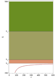
(b)

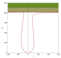
Figure 1. Plot of the implicit curve $\mathcal{C}$ with Maple for the sequential phosphorylation in Markevich et al. (2004). (a): The bounds $500,\alpha_{1},\alpha_{2},\alpha_{3}$ for $c>0,x_{1}>390$, where the intervals $[\alpha_{i+1},\alpha_{i}]$ have different colors. (b): The picture for $-200<c<300,x_{1}>0$.

The first part of Theorem 2.3 is based on the following well known result, which follows from the Implicit Function Theorem (IFT). As we haven’t found any good reference for its proof, we sketch it in the Appendix for the convenience of the reader.

Lemma 2.4.

Let $p=p(c,x_{1})\in I$ with positive degree $n$ in $c$ and for any $\beta$ consider the set $\mathcal{C}_{\beta}$ defined in (7). Then, the cardinality $\#\mathcal{C}_{\beta}$ of $\mathcal{C}_{\beta}$ is the same for all $\beta$ in a connected component $\Omega$ of the complement of the zeros of the resultant $R_{n}$ in $\mathbb{R}$.

Under the hypotheses of Lemma 2.1, there exists a polynomial $p\in I$ with positive degree in $x_{1}$. As we remarked before, unless $x_{1}$ takes only a finite number of values, this polynomial will also have positive degree in $c$, which is required in Theorem 2.3. Indeed, as also $R_{n}$ is required to be non identically zero, if the degree of $p$ in $x_{1}$ is not positive, then $R_{n}$ would be a nonzero constant. Therefore, $R_{n}$ would have no roots and the result is void.

We observe that there is no need to have the exact values of the roots of $R_{n}$ (which are in general impossible to get). It is enough to find (small) intervals that isolate the roots (say, of radius $\delta$ around each $\alpha_{j}$) and then pick the values $\beta_{j}$ between the extreme points of these intervals. The bound we get this way is slightly bigger (e.g. $\alpha_{k}+\delta$), but computable. On the other side, in order to check the emptiness of $\mathcal{C}_{\alpha_{i}}\cap\ell_{1}(\mathbb{R}_{\geq 0}^{s})$, there are symbolic procedures available to determine the number of real roots of zero dimensional ideals subject to real polynomial inequalities, for example the libraries for real roots implemented in Singular (Singular;Tobis, 2005). Namely, if $\alpha_{i}$ is the unique root of $R_{n}$ in the rational interval $(\xi_{1},\xi_{2})$, then one needs to check that there are no real solutions $c$ satisfying the conditions

$$R_{n}(x_{1})=p(c,x_{1})=0,\,\xi_{1}<x_{1}<\xi_{2},\,c\in J.$$

Notice also that the bounds in Theorem 2.3 hold in principle for fixed values of $b_{2},\dots,b_{r}$, but in theory one could get (by a variant of Lemma 2.1 under natural hypotheses) a polynomial $p$ depending on these parameters (and even on the rate constants). We exemplify this in § 3.5.

Our methods can be adapted, besides mass-action kinetics systems, to standard modelings with autonomous rational dynamical systems, like power law dynamics with integer exponents or Michaelis-Menten kinetics.

3. Application to an enzymatic network

In this section, we illustrate the use of Theorem 2.3 to find nontrivial bounds in example (3) from Markevich et al. (2004), which models an enzymatic network with sequential phosphorylations and dephosphorylations. We also use this example to explain the need for the hypotheses and the scope of Theorem 2.3. We moreover use the tools presented in Section 2 to get a more detailed study of the system.

3.1. The equations

We name the species concentrations in network (3) by

$$\begin{array}[]{llll}x_{1}\leftrightarrow[\text{Mpp}],&x_{4}\leftrightarrow[\text{M-MAPKK}],&x_{6}\leftrightarrow[\text{Mpp-MKP3}],&x_{10}\leftrightarrow[\text{MAPKK}],\\ x_{2}\leftrightarrow[\text{Mp}],&x_{5}\leftrightarrow[\text{Mp-MAPKK}],&x_{7}\leftrightarrow[\text{Mp-MKP3}],&x_{11}\leftrightarrow[\text{MKP3}].\\ x_{3}\leftrightarrow[\text{M}],&&x_{8}\leftrightarrow[\text{Mp-MKP3}^{*}],&\\ &&x_{9}\leftrightarrow[\text{M-MKP3}],&\\ \end{array}$$

Then, the differential equations of the system under mass–action kinetics are:

$$f_{1} =k_{4}x_{5}-h_{1}x_{1}x_{11}+h_{-1}x_{6}$$

$$f_{2} =k_{2}x_{4}-k_{3}x_{2}x_{10}+k_{-3}x_{5}+h_{3}x_{7}-(h_{-3}+h_{4})x_{2}x_{11}+h_{-4}x_{8}$$

$$f_{3} =-k_{1}x_{3}x_{10}+k_{-1}x_{4}-h_{-6}x_{3}x_{11}+h_{6}x_{9}$$

$$f_{4} =k_{1}x_{3}x_{10}-(k_{-1}+k_{2})x_{4}$$

$$f_{5} =k_{3}x_{2}x_{10}-(k_{-3}+k_{4})x_{5}$$

$$f_{6} =h_{1}x_{1}x_{11}-(h_{-1}+h_{2})x_{6}$$

$$f_{7} =h_{2}x_{6}-h_{3}x_{7}+h_{-3}x_{2}x_{11}$$

$$f_{8} =h_{4}x_{2}x_{11}-(h_{-4}+h_{5})x_{8}$$

$$f_{9} =h_{5}x_{8}-h_{6}x_{9}+h_{-6}x_{3}x_{11}$$

$$f_{10} =-k_{1}x_{3}x_{10}+(k_{-1}+k_{2})x_{4}-k_{3}x_{2}x_{10}+(k_{-3}+k_{4})x_{5}$$

$$f_{11} =-h_{1}x_{1}x_{11}+h_{-1}x_{6}+h_{3}x_{7}-(h_{-3}+h_{4})x_{2}x_{11}+h_{-4}x_{8}+h_{6}x_{9}-h_{-6}x_{3}x_{11},$$

and the conservation relations can be given as:

$$L_{1}=x_{4}+x_{5}+x_{10}-\text{MAPKK}_{tot} =0$$

$$L_{2}=x_{1}+x_{2}+x_{3}+x_{4}+x_{5}+x_{6}+x_{7}+x_{8}+x_{9}-\text{M}_{tot} =0$$

$$L_{3}=x_{6}+x_{7}+x_{8}+x_{9}+x_{11}-\text{MKP3}_{tot} =0.$$

We set the reaction constants as in the SI in Markevich et al. (2004):

$k_{1}=0.02,k_{-1}=1,k_{2}=0.01,k_{3}=0.032,k_{-3}=1,k_{4}=15$, $h_{1}=0.045,h_{-1}=1,h_{2}=0.092,h_{3}=1$, $h_{-3}=0.01,h_{4}=0.01,h_{-4}=1,h_{5}=0.5,h_{6}=0.086,h_{-6}=0.0011$, and fix $\text{M}_{tot}=500,\text{MKP3}_{tot}=100$. We let

(8) $$\ell_{1} =x_{4}+x_{5}+x_{10},$$

$$\ell_{2} =x_{1}+x_{2}+x_{3}+x_{4}+x_{5}+x_{6}+x_{7}+x_{8}+x_{9},$$

$$\ell_{3} =x_{6}+x_{7}+x_{8}+x_{9}+x_{11}.$$

Denote by $I$ the ideal generated by the polynomials $f_{1},f_{2},\dots,f_{s},\ell_{1}-c,\ell_{2}-500,\ell_{3}-100$.

3.2. The implicit dose-response curve associated to $x_{1}$ and MAPKK_tot

We first take the output $x_{1}:=$[M_pp] and the input $c:=$MAPKK_tot. Note that the trivial bound along trajectories is equal to $\text{M}_{tot}=500$.

Via Gröbner basis elimination methods in Singular we find that the intersection of $I$ with the ring of polynomials in the variables $x_{1}$ and $c$ is generated by the following polynomial $p=p(c,x_{1})=\sum_{i=0}^{4}p_{i}(x_{1})c^{i}$ with degree $n=4$ in $c$, with coefficients:

$$p_{4} =259578228128346056201372100x_{1}^{4}-91228131699664084594014546000x_{1}^{3}$$

$$-5318853461888966748775026000000x_{1}^{2}-107717641535472295661334000000000x_{1}$$

$$-983693913810151954410000000000000,$$

$$p_{3} =-1279181837636260017061541940x_{1}^{5}+217225713953041585784715122400x_{1}^{4}$$

$$+111432561952880309835561787920000x_{1}^{3}+4108996025231164151414890560000000x_{1}^{2}$$

$$+32909012963892503562524400000000000x_{1},$$

$$p_{2} =1651342827133987314483094029x_{1}^{6}-57239961872970579411022490540x_{1}^{5}$$

$$-172636108121018180634948973020000x_{1}^{4}-29157440247951003530589295575600000x_{1}^{3}$$

$$-655794481210925030267002164000000000x_{1}^{2}$$

$$-3924727591361860067680350000000000000x_{1},$$

$$p_{1} =-23638737258912336217603357320x_{1}^{6}+40121950932074520838137058397200x_{1}^{5}$$

$$-10189010265838070554939750993840000x_{1}^{4}$$

$$-458846180258284496202210449400000000x_{1}^{3}$$

$$-3875235380408791071737337000000000000x_{1}^{2}\;\text{and}$$

$$p_{0} =13225968047392416670218470096400x_{1}^{6}-11693689998883687367816615216864000x_{1}^{5}$$

$$+2446220546414268358687194986380000000x_{1}^{4}$$

$$+67830374851435086233478373420000000000x_{1}^{3}$$

$$+440552682490042857644978250000000000000x_{1}^{2}.$$

It is clear that one does not want to find this polynomial by hand. But once we have it, we can extract interesting conclusions.

The resultant $R_{4}$ of $p$ and $\frac{\partial p}{\partial c}$, thought of as polynomials in $\mathbb{R}[x_{1}][c]$ of degrees $4$ and $3$, is a polynomial in $\mathbb{R}[x_{1}]$ of degree $38$ with big coefficients. $R_{4}$ has fourteen nonreal roots (of which eight are double roots), three negative roots (of which one is a double root), four positive real roots (of which two are double roots) and has $x_{1}=0$ as a root of multiplicity six. The values of the positive roots are approximately:

$$\alpha_{1}\approx 454.01,\;\alpha_{2}\approx 410.37,\;\alpha_{3}\approx 404.67,\,\text{and}\;\alpha_{4}\approx 312.56.$$

Following Theorem 2.3, we can choose for example $\beta_{1}=470$, $\beta_{2}=420$, $\beta_{3}=405$ and $\beta_{4}=350$ which satisfy the inequalities $\beta_{1}>\alpha_{1}>\beta_{2}>\alpha_{2}>\beta_{3}>\alpha_{3}>\beta_{4}>\alpha_{4}$. We find that $p(\beta_{1},c)$ and $p(\beta_{2},c)$ have no real roots. Since the nonzero coefficients of $\ell_{1}$ in (8) are positive, we have $J=[0,+\infty)$, and $\mathcal{C}_{\alpha_{1}}\cap J=\mathcal{C}_{\alpha_{2}}\cap J=\emptyset$. This makes $\alpha_{2}$ a nontrivial upper bound for $x_{1}$ at steady state by the first part of Theorem 2.3, which is sharper than the trivial bound $500$.

The leading coefficient $p_{4}$ equals $3916521308700$ times the polynomial

$$(819x_{1}^{2}-308940x_{1}-9100000)(80925216157x_{1}^{2}+2085327062000x_{1}+27600573000000).$$

As the second factor has no real roots, the real roots of $p_{4}$ are the roots of $819x_{1}^{2}-308940x_{1}-9100000$, which are, $\alpha_{3}$ and another one approximately equal to $-27.46$. As $J=[0,+\infty)$, we consider the zeros of $p(0,x_{1})$, which are approximately $-13.52$, $-11.85$ and $0$. They are clearly less than $\alpha_{3}$, and $p(\alpha_{2},c)=0$ for $c\approx-70.4$, which is negative. Then, by the second part of Theorem 2.3, $\alpha_{3}$ is a better nontrivial upper bound for $x_{1}$ at steady state (since $\alpha_{3}<\alpha_{2}<500$).

If instead, we consider $x_{3}$ as output variable, by elimination in $I$ of all variables except for $x_{3}$ and $c$, we obtain a polynomial $q(x_{3},c)\in I$ with degree $n=4$ in the variable $c$. Its leading coefficient $q_{4}$ is

$$375791837967x_{3}(890177377727x_{3}^{2}+81709195989640x_{3}+3800250418891200).$$

Note that ${q}_{4}$ has no positive real roots, which makes us unable to apply the second part of Theorem 2.3. The resultant $R_{4}$ of $q$ and $\frac{\partial q}{\partial c}$, thought of as polynomials in $\mathbb{R}[x_{3}][c]$ of degrees $4$ and $3$, is a polynomial in $\mathbb{R}[x_{3}]$ of degree $38$. $R_{4}$ has only one positive real root which is approximately $\alpha_{1}\approx 440.55$. We can see that $q(450,c)$ has no real roots. This makes $\alpha_{1}$ a nontrivial upper bound for $x_{3}$ at steady state by the first part of Theorem 2.3.

3.3. Depicting the implicit dose-response curve

We depict in Figures 2 and 3 the results we have obtained for the sequential dual phosphorylation–dephosphorylation cycle from Markevich et al. (2004) using the implicit dose-response curve ${\mathcal{C}}=\{(c,x_{1})~{}|~{}p(c,x_{1})=0\}$, plotted with Maple. In Figure 2 we can see the curve $\mathcal{C}$ in the positive quadrant (the usual dose-response curve). This curve represents the relation between the input $\text{MAPKK}_{tot}$ ($c$) and the output Mpp ($x_{1}$) at steady state when both take positive values. The difference between the trivial and the nontrivial bounds is marked with color. In Figure 3(a) we can see that the nontrivial bound is not an upper bound for negative values of $c$, where $\alpha_{2}$ gives a slightly bigger upper bound. Figure 3(b) shows the curve $\mathcal{C}$ for negative values of $x_{1}$.

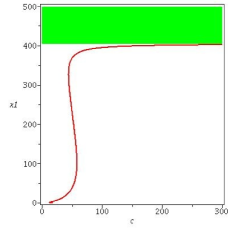
Figure 2. The curve $\mathcal{C}$ in the positive quadrant. This curve represents the relation between the input $\text{MAPKK}_{tot}$ ($c$) and the output Mpp ($x_{1}$) at steady state when both take positive values. The difference between the trivial and the improved bound is marked with color.

(a)

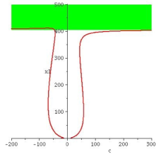
(b)

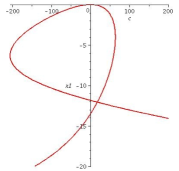
Figure 3. The algebraic curve $\mathcal{C}$ in different quadrants.

Note that for small values $c^{*}$ there are four real values of $x_{1}$ satisfying the degree $4$ polynomial equation $p(c^{*},x_{1})=0$ and in a certain range, approximately for $c^{*}$ in the interval $(44.43,58.33)$, there are $3$ positive solutions. In fact, the system shows multistationarity in this range, and the middle values correspond to unstable steady states. Figure 4 below presents the differences and similarities between the approximate plot of the implicit curve $\mathcal{C}$ and the curve featuring hysteresis obtained via numerical ode simulation with MATLAB. So, the black curve in Figure 4 (a) approximates all the positive real zeros $(c,x_{1})$ of $p$. On the other side, the curves (b), (c), (d) are produced as approximate limit values via numerical integration of the ode system at different initial values. In Figure 4 (c) and (d), the two curves in (b) are depicted separately. The initial values for the curve in (c) vary with $c$ and are $x_{10}^{*}=$[MAPKK]$=c$, $x_{3}^{*}=$[M]$=500$, $x_{11}^{*}=$[MKP3]$=100$, and the other variables are set to zero. The value of $x_{1}$ represented is (approximately) the equilibrium value (computed for a big enough value of time $t$). The curve in (d) should be read “backwards”, starting at $c=100$ with the corresponding equilibrium point of the curve in (c) as initial state. At each step, the total amount of [MAPKK] is reduced from the previous equilibrium, keeping the same stoichiometric compatibility class for each value of $c$, until $c=0$ is reached. Two “fake” traces appear in this usual numerical picture: those that go from the lower stable values of $x_{1}$ to the higher stable values of $x_{1}$ and back, which are produced by an intent of the plotter to interpolate continuously the solutions of the simulations (there are also some inaccuracies due to the numeric approximation). (See the Supplementary Material we provide for the MATLAB script used to produce Figure 4 (b), (c) and (d).) Note that the middle unstable steady state values in the black curve in (a) (in the multistationarity range) are not taken as the initial values, and they do not occur in the blue and green curves in (b).

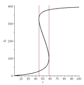
(a)	(b)
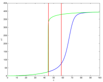
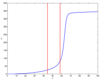
(c)	(d)

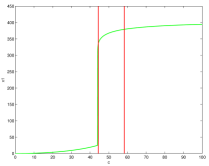
Figure 4. The dose-response curves in the positive orthant with the vertical lines $c=44.43$ and $c=58.33$. (a): The plot of the implicit curve $\mathcal{C}$ in black with Maple. (b): The standard hysteresis simulation diagram with MATLAB, which is the superposition of the curves in (c) and (d). (c): The blue curve in (b) from the lower steady state values of $x_{1}$ to the higher steady state values. (d): The green curve in (b) from the higher steady state values of $x_{1}$ to the lower steady state values.

3.4. Taking $x_{2}$ as output variable

If we now follow the same procedure but eliminating all variables except for $x_{2}$ and $c$, we obtain a polynomial $q(x_{2},c)$, again with degree $4$ in the variable $c$. The resultant $R_{4}$ of $q$ and $\frac{\partial q}{\partial c}$, thought of as polynomials in $\mathbb{R}[x_{2}][c]$, is a polynomial in $\mathbb{R}[x_{2}]$ of degree $38$ with only six positive real roots. The values of these positive roots are approximately $\alpha_{1}\approx 15.2$, $\alpha_{2}\approx 8.49$, $\alpha_{3}\approx 3.02$, $\alpha_{4}\approx 2.1347$, $\alpha_{5}\approx 2.1345$, and $\alpha_{6}\approx 2.1263$.

As $q(20,c)$ has no real roots, $\alpha_{1}$ is a nontrivial upper bound for $x_{2}$ at steady state by the first part of Theorem 2.3. To use the second part of this theorem, we must focus on the roots of the leading coefficient in $c$, which has no positive root. Hence, the only nontrivial bound we can find is $\alpha_{1}\approx 15.2$.

The corresponding implicit dose-response curve $\mathcal{C}^{\prime}=\{(c,x_{2})|q(c,x_{2})=0\}$ has the unexpected shape featured in Figure 6(a). For $c^{*}$ in the same approximate range $(44.43,58.33)$, there are more than one positive solutions $x_{2}$ to the polynomial equation $q(c^{*},x_{2})=0$. The higher values correspond to unstable steady states. The lower values values cannot be completed to a nonnegative steady state, as we now explain with the help of Figure 5. We remark that those points do not lie on a line, as the approximate picture seems to show.

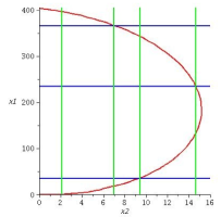
Figure 5. The curve $g(x_{1},x_{2})=0$ (red), the horizontal lines that represent $p(50,x_{1})=0$ and the vertical lines that represent $q(50,x_{2})=0$, in the positive orthant

We can instead eliminate from $I$ all variables (including $c$) but $x_{1}$ and $x_{2}$. We computed with Singular a nonzero polynomial $g=g(x_{1},x_{2})\in I$, which relates the values of $x_{1}$ and $x_{2}$ at steady state for any value of $c$. We pick the value $c^{*}=50$ in the multistationarity range. Figure 5 depicts:

• the (approximate) curve $\{g=0\}$,

• the horizontal lines defined by $p(50,x_{1})=0$,

• the vertical lines defined by $q(50,x_{2})=0$,

in the nonnegative orthant of the $(x_{2},x_{1})$-plane. For any steady state for which $c=50$, the values of its second and first coordinates have to be in the intersection of these three pictures. We see that no point with $x_{2}$ close to $2$ satisfies this property.

One can now guess the shape of the hysteresis simulation diagram (produced with MATLAB), which is shown in Figure 6(b). Again, it is interesting to detect the “fake” traces in the plot, when comparing with the implicit dose-response curve $\mathcal{C}^{\prime}$ in Figure 6(a).

(a)

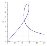
(b)

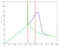
Figure 6. The curve $q(c,x_{2})=0$ in the positive orthant with the lines $c=44.43$ and $c=58.33$ in red. (a): The plot of the implicit curve with Maple. (b): Simulation with MATLAB.

3.5. Moving the parameters

As we remarked in Section 2, by a variant of Lemma 2.1, one could get a polynomial $p$ in the ideal $I$ depending on some of the parameters $b_{2},\dots,b_{r}$ or some rate constants. In theory, this is possible. In practice, even if one could compute $p$ effectively, the output might be too big to be understood. For our running example, we also consider as variables (besides the $x_{i}$’s) the following: $c=b_{1}$ (MAPKK_tot), $b_{2}$ (M_tot), $b_{3}$ (MKP3_tot), and $h_{1}$.

In this case, we can compute a polynomial $p=p(c,b_{2},b_{3},h_{1},x_{1})$ in the parametric steady state ideal (considered in $\mathbb{R}[c,b_{2},b_{3},h_{1},x_{1},\dots,x_{11}]$) of total degree $13$, degree $6$ in $x_{1}$ and degree $4$ in $c$. The coefficient $p_{4}(b_{2},b_{3},h_{1},x_{1})$ of $c^{4}$ in $p$ equals:

$$(\eta_{1}+\eta_{2}x_{1}h_{1}+\eta_{3}x_{1}^{2}h_{1}^{2})(4095x_{1}^{2}h_{1}+4118x_{1}h_{1}b_{3}-4095x_{1}h_{1}b_{2}+4095x_{1}-4095b_{2}),$$

with $\eta_{1}=55891160325>0$, $\eta_{2}=93839717790>0$, and $\eta_{3}=80925216157>0$. The biggest positive asymptote $x_{1}=\alpha$ is given by the only positive root $\alpha$ of the right factor, which is easily seen to be smaller than the trivial bound $b_{2}$. Moreover, the difference $b_{2}-\alpha$ is the following positive quantity:

(9) $$b_{2}-\alpha=\dfrac{\mu-\sqrt{\mu^{2}-4\nu h_{1}^{2}b_{2}b_{3}}}{2h_{1}},$$

where $\mu=1+h_{1}(b_{2}+\nu b_{3})$ and $\nu=\frac{4118}{4095}$. For fixed $b_{2}$ and $b_{3}$, we can see for instance that $\alpha$ tends to the trivial bound $b_{2}=\text{M}_{tot}$ when the dephosphorylation reaction constant $h_{1}$ tends to zero, as expected. In general, one can try to perform the computations keeping a few relevant parameters as variables, to get a precise implicit description of the dependence of the steady state values on these parameters.

4. DISCUSSION

We have introduced a novel approach for the study of dose-response curves, that is, for the relation between steady state coordinates and input variables in autonomous polynomial dynamical systems, via implicit curves. This analysis is possible regardless the absence of explicit expressions or the presence of multistationarity and gives explicitly the implicit relations between the input and the output.

As an application, we made a thorough study of one of the enzymatic mechanisms in Markevich et al. (2004), where we obtained nontrivial bounds at steady state. We also used this example to point out how to understand the usual pictures featuring hysteresis and to show that the implicit curves can be too difficult to be obtained “by hand” but they can nevertheless be used to extract interesting conclusions on the behavior of the system.

Appendix

We include the proofs of Lemma 2.1, Lemma 2.4 and Theorem 2.3.

Proof of Lemma 2.1.

The proof uses basic results on the dimension of algebraic varieties, that can be found for instance in (Shafarevich, 1994, Chapter 1,§ 6). As we remarked after the statement of Lemma 2.1, the ideal $I$ can be generated by $s$ polynomials in $s+1$ variables, and so its dimension $d$ is at least $1$. Consider the projection map $\pi(c,x_{1},\dots,x_{s})=c$ from the variety $V(I)$ of zeros of $I$ in $\mathbb{C}^{s+1}$. If there exists a nonzero polynomial $q\in I\cap\mathbb{R}[c]$, the image of $V(I)$ would be contained in the zero set of $q$ in $\mathbb{C}$ and would be therefore of dimension $0$. By hypothesis, the fiber over any of those points has also dimension $0$ but then from the Fibre Dimension Theorem we would get $0\geq d-0\geq 1$, a contradiction. Therefore, the image is dense in $\mathbb{C}$ and so its closure has dimension $1$. Again, by the same Theorem, we deduce that the dimension of $I$ equals $1$. This implies that, given $2$ (or more) variables, it is possible to find a nonzero polynomial in those variables in the ideal. In particular, we can find a nonzero polynomial $p=p(c,x_{1})$ in $I\cap\mathbb{R}[c,x_{1}]$ with positive degree in $x_{1}$. ∎

Proof of Lemma 2.4.

It is enough to show that for any $\beta\in\Omega$ there exists a neighborhood where the cardinality is constant. By Lemma 2.2, we have that $p_{n}(\beta)\neq 0$ and $\frac{\partial p}{\partial c}(c,\beta)\neq 0$ for all $c$ such that $p(c,\beta)=0$. Let $d=\#\mathcal{C}_{\beta}$ and call $\mathcal{C}_{\beta}=\{c^{1},\dots,c^{d}\}$. Using the IFT, it is possible to find an open set $V$ around $\beta$ and, for $1\leq i\leq d$, open sets $U_{i}$ around each $c^{i}$ with $U_{i}\cap U_{j}=\emptyset$ if $i\neq j$, and smooth functions $g_{i}:V\to U_{i}$ in $\mathcal{C}^{1}$ such that

$$\{(g_{i}(x_{1}),x_{1})~{}|~{}x_{1}\in V\}=\{(c,x_{1})\in U_{i}\times V~{}|~{}p(c,x_{1})=0\}.$$

Thus, for all $x_{1}\in V$ we have that $\#\mathcal{C}_{x_{1}}\geq d$.

Suppose there exists a sequence $\gamma_{m}\to\beta$ for $m\to\infty$ with $\gamma_{m}\in V$ and $\#\mathcal{C}_{\gamma_{m}}>d$. For every $m$, choose a point $c_{m}$ with $p(c_{m},\gamma_{m})=0$ and $c_{m}\neq g_{i}(\gamma_{m})$ for all $i=1,\dots,d$. Since $x_{1}=\beta$ is not an asymptote, the sequence $(c_{m})$ is bounded and thus there exists a convergent subsequence of $((c_{m},\gamma_{m}))$ which converges to a point $(c^{*},\beta)$. But then $p(c^{*},\beta)=0$ and $c^{*}$ is different from $c^{1},\dots,c^{d}$, a contradiction. ∎

Proof of Theorem 2.3.

Let $\alpha_{1}>\alpha_{2}>\dots>\alpha_{m}$ be the real zeros of $R_{n}$, and $k\in\{1,\dots,m\}$, $\beta_{1},\dots,\beta_{k}$ be as in the hypotheses of Theorem 2.3. The open intervals $(\alpha_{i},\alpha_{i-1})$ for $1\leq i\leq k$ and $\alpha_{0}:=+\infty$ are connected components of the complement of the zeros of $R_{n}$. By Lemma 2.4, $\#\mathcal{C}_{x_{1}}=\#\mathcal{C}_{\beta_{i}}=0$ for all $x_{1}\in(\alpha_{i},\alpha_{i-1})$ for $1\leq i\leq k$. There are no zeros of $p$ with $x_{1}=\alpha_{i}$ ($1\leq i\leq k$) because $\mathcal{C}_{\alpha_{i}}\cap J=\emptyset$ by hypothesis, which means that there are no nonnegative steady states with $x_{1}=\alpha_{i}$. Therefore, we have $x_{1}<\alpha_{k}$ at any nonnegative steady state. This is, $\alpha_{k}$ is an upper bound for $x_{1}$ at steady state.

Let $\alpha$ be as in the second part of Theorem 2.3. Denote by $X$ the set $X:=\{x_{1}>\alpha:\textrm{there exists}\;c\in J\;\text{with}\;p(c,x_{1})=0\}$. By the first part of the theorem, we have $x_{1}<\alpha_{k}$ for all $x_{1}$ in $X$. Suppose $X\neq\emptyset$, and let us call $\mu$ the supremum of $X$. If $x_{1}=\mu$ were an asymptote, we would have $p_{n}(\mu)=0$, which is not possible because $\mu>\alpha$. Then, for any sequence $((c^{(m)},x_{1}^{(m)}))\subset\mathcal{C}$ with $x_{1}^{(m)}\in X$, $x_{1}^{(m)}\to\mu$, and $c^{(m)}\in J$, there exists a convergent subsequence such that the first coordinates tend to some $c^{*}\in J$ ($J$ is closed). Since $p$ is continuous, we have $p(c^{*},\mu)=0$, and by hypothesis, as $\alpha<\mu\leq\alpha_{k}$, $\frac{\partial p}{\partial c}(\mu,c^{*})\neq 0$. Then, by the IFT, there exist $\delta>0$ and a smooth function $g$ such that $p(g(x_{1}),x_{1})=0$ for all $x_{1}\in(\mu,\mu+\delta)$. If $J=\mathbb{R}$, this is impossible because $\mu$ is the supremum. If $J=[0,+\infty)$, then $\mu$ is a maximum and $c^{*}=0$, but this is not possible by hypothesis, since $p(0,x_{1})\neq 0$ for all $x_{1}>\alpha$. Therefore, $X=\emptyset$ and $x_{1}\leq\alpha$ at every nonnegative steady state.

∎

References

- Cox et al. (2007) Cox D., Little J., O’Shea D. (2007), Ideals, varieties and algorithms. Undergraduate Texts in Mathematics, Third Edition, Springer, New York.
- Singular (0000) Decker W., Greuel G.-M., Pfister G., Schönemann H. (2012), Singular 3-1-6 — A computer algebra system for polynomial computations. http://www.singular.uni-kl.de
- Feinberg (1979) Feinberg M. (1979), Lectures On Chemical Reaction Networks. Ohio State University. http://www.crnt.osu.edu/LecturesOnReactionNetworks
- Feinberg and Horn (1977) Feinberg M., Horn F. (1977), Chemical mechanism structure and the coincidence of the stoichiometric and kinetic subspaces. Arch. Ration. Mech. Anal. 66(1), pp. 83–97.
- Feliu and Wiuf (2012) Feliu E., Wiuf C. (2012), Enzyme-sharing as a cause of multi-stationarity in signalling systems. J. R. Soc. Interface 9(71), pp. 1224–1232.
- Feliu et al. (2012) Feliu E., Knudsen M., Andersen L., Wiuf C. (2012), An algebraic approach to signaling cascades with layers. Bull. Math. Biol. 74(1), pp. 45–72.
- Flockerzi et al. (2013) Flockerzi D., Holstein K., Conradi C. (2013), N-site phosphorylation systems with 2N-1 steady states. Available at arXiv:1312.4774.
- Gelf′and et al. (1994) Gelf′and I.,Kapranov M., Zelevinsky A. (1994), Discriminants, Resultants and Multidimensional Determinants. Birkhäuser, Boston.
- Horn and Jackson (1972) Horn F., Jackson R. (1972), General mass action kinetics. Arch. Ration. Mech. Anal., 47(2), pp. 81–116.
- Karp et al. (2012) Karp R., Pérez Millán M., Dasgupta T., Dickenstein A., Gunawardena J. (2012), Complex-linear invariants of biochemical networks. J. Theor. Biol. 311, pp. 130–138.
- Maple (0000) Maple 17 (2013), Maplesoft, a division of Waterloo Maple Inc., Waterloo, Ontario.
- Markevich et al. (2004) Markevich N., Hoek J., Kholodenko B. (2004), Signaling switches and bistability arising from multisite phosphorylation in protein kinase cascades. J. Cell Biol. 164(3), pp. 353–359.
- MATLAB (0000) MATLAB (2014), version 8.3.0. Natick, Massachusetts: The MathWorks Inc.
- Pérez Millán et al. (2012) Pérez Millán M., Dickenstein A., Shiu A., Conradi C. (2012), Chemical reaction systems with toric steady states. Bull. Math. Biol. 74(5), pp. 1027–1065.
- Shafarevich (1994) Shafarevich, I. (1994), Basic algebraic geometry. 1. Varieties in projective space. Second edition. Springer-Verlag, Berlin.
- Tobis (2005) Tobis E. A. (2005), Libraries for Counting Real Roots, Reports on Computer Algebra (ZCA, University of Kaiserslautern) 34.
- Vol′pert and Hudjaev (1985) Vol′pert A. I., Hudjaev S. I. (1985), Analysis in classes of discontinuous functions and equations of mathematical physics. volume 8 of Mechanics: Analysis. Martinus Nijhoff Publishers, Dordrecht.
- Wang and Sontag (2008) Wang L., Sontag E. (2008), On the number of steady states in a multiple futile cycle. J. Math. Biol. 57(1), pp. 29–52.