Is the Milky Way’s Hot Halo Convectively Unstable?

Abstract

We investigate the convective stability of two popular types of model of the gas distribution in the hot Galactic halo. We first consider models in which the halo density and temperature decrease exponentially with height above the disk. These halo models were created to account for the fact that, on some sight lines, the halo’s X-ray emission lines and absorption lines yield different temperatures, implying that the halo is non-isothermal. We show that the hot gas in these exponential models is convectively unstable if $\gamma<3/2$, where $\gamma$ is the ratio of the temperature and density scale heights. Using published measurements of $\gamma$ and its uncertainty, we use Bayes’ Theorem to infer posterior probability distributions for $\gamma$, and hence the probability that the halo is convectively unstable for different sight lines. We find that, if these exponential models are good descriptions of the hot halo gas, at least in the first few kiloparsecs from the plane, the hot halo is reasonably likely to be convectively unstable on two of the three sight lines for which scale height information is available. We also consider more extended models of the halo. While isothermal halo models are convectively stable if the density decreases with distance from the Galaxy, a model of an extended adiabatic halo in hydrostatic equilibrium with the Galaxy’s dark matter is on the boundary between stability and instability. However, we find that radiative cooling may perturb this model in the direction of convective instability. If the Galactic halo is indeed convectively unstable, this would argue in favor of supernova activity in the Galactic disk contributing to the heating the hot halo gas.

1. INTRODUCTION

X-ray observations indicate the presence of hot gas above the disk of our Galaxy, in the halo, with temperatures of $\sim$$(\mbox{1--3})\times 10^{6}$ K. Evidence for this hot gas comes from observations of the diffuse soft X-ray background (SXRB) emission (e.g., Kuntz & Snowden, 2000; Yoshino et al., 2009; Henley & Shelton, 2013), and absorption lines from highly ionized metals in the X-ray spectra of active galactic nuclei (e.g., Nicastro et al., 2002; Rasmussen et al., 2003; Yao & Wang, 2007; Hagihara et al., 2010; Gupta et al., 2012; Miller & Bregman, 2013). The hot halo gas is thought to be due to supernova-driven outflows from the Galactic disk (e.g., Shapiro & Field, 1976; Norman & Ikeuchi, 1989; Joung & Mac Low, 2006; Hill et al., 2012) and/or infall of extragalactic gas (e.g., Toft et al., 2002; Rasmussen et al., 2009; Crain et al., 2010), but the relative importance of these two processes remains uncertain (Henley et al., 2010; Henley & Shelton, 2013).

In this paper, we consider the question of energy transport in the hot halo. In particular, we investigate whether or not the hot halo gas is convectively unstable. In a so-called galactic fountain (Shapiro & Field, 1976; Bregman, 1980), a convective flow is expected to be set up by supernova heating: the heated gas moves from the disk into the halo, either by superbubbles breaking out of the disk (e.g., Mac Low et al., 1989) or by regions of hot gas rising buoyantly (Avillez & Mac Low, 2001), and then subsequently cools and falls back to the disk. However, while several different models for the density and temperature distributions of the hot halo have recently been proposed, to the best of our knowledge no one has investigated the convective stability of these models. Our goal here is to help build a more complete picture of the physical processes occurring in the halo.

Whether or not a halo model is convectively unstable depends on the density and temperature distributions of the gas, and there is some disagreement regarding the best model to describe these distributions. Such models fall mainly into two broad categories, which we refer to as exponential and extended halo models (in this paper, we will examine halo models from both categories). Wang & Yao (2012, and references therein) argue in favor of the former type of model, saying that the X-ray observations are best described by a model in which the hot halo plasma is concentrated relatively close to the disk, with an exponential scale height of a few kiloparsecs. However, others argue that the X-ray observations indicate a more extended hot halo ($\gtrsim$100 kpc in extent; e.g., Gupta et al., 2012, 2013; Miller & Bregman, 2013). There is also indirect evidence for an extended halo, such as the lack of gas in satellite galaxies and the confinement of high-velocity clouds (Fang et al., 2013, and references therein). In reality, the halo may consist of a combination of exponentially distributed gas close to the disk and more extended, lower-density gas (Yao & Wang, 2007).

In Section 2, we will discuss the arguments for and against the exponential and extended halo models. As the global morphology and extent of the hot halo are uncertain, we will consider the convective stability of both types of model, in Sections 3 and 4, respectively. We discuss our results in Section 5, and conclude with a summary in Section 6.

2. MODELS OF THE MILKY WAY’S HOT HALO

2.1. Exponential Halo Models

Yao & Wang (2007) argued that the observed halo O VII/O VIII column density ratio (measured from the high-resolution Chandra grating spectrum of Mrk 421) and the diffuse O VII/O VIII emission ratio (from a microcalorimeter spectrum of the SXRB; McCammon et al. 2002) implied different halo temperatures, implying that the halo is non-isothermal (see the first row of Table 2.1). Instead, Yao & Wang (2007) found that the observations could be described by a disk-like halo model in which the number density, $n$, and temperature, $T$, decreased exponentially with height, $z$:

$$n(z) = n_{0}\exp\left(-\frac{z}{h_{n}\xi}\right),$$ (1)

$$T(z) = T_{0}\exp\left(-\frac{z}{h_{T}\xi}\right),$$ (2)

where $n_{0}$ and $T_{0}$ are the midplane values, $h_{n}$ and $h_{T}$ are the scale heights (assumed to be positive), and $\xi$ is the hot gas filling factor (assumed to be a constant).

Table 1Observed Halo Temperatures, Observed Values of $\gamma\equiv h_{T}/h_{n}$, and Convective Instability Probabilities

Sight line	$\log T_{\mathrm{emis}}$	$\log T_{\mathrm{abs}}$	$\gamma$	Reference	$P(\gamma<3/2)$
	(K)	(K)
(1)	(2)	(3)	(4)	(5)	(6)
Mrk 421	$\sim$6.33	6.16 (6.10, 6.21)	0.29 ($<1.63$)	1	0.89
	6.32 (6.29, 6.35)	6.16 (6.08, 6.24)	$\cdots$	2	$\cdots$
LMC X-3	6.38 (6.34, 6.40)	6.11 (5.90, 6.30)	0.5 (0.1, 1.7)	3	0.87
PKS 2155$-$304	6.33 (6.31, 6.35)	6.27 (6.24, 6.29)	2.44 (1.03, 3.55)	4	0.15
	6.36 (6.34, 6.38)	6.27 (6.22, 6.32)	$\cdots$	2	$\cdots$

References. — 1. Temperatures from Yao & Wang (2007); $\gamma$ from Sakai et al. (2012). 2. Gupta et al. (2013). 3. Yao et al. (2009), Table 3. $T_{\mathrm{emis}}$, $T_{\mathrm{abs}}$, and $\gamma$ are from rows 1–3 of that table, respectively. 4. Hagihara et al. (2010). $T_{\mathrm{emis}}$, $T_{\mathrm{abs}}$, and $\gamma$ are from row 3 of Table 4, row 2 of Table 3, and row 1 of Table 7, respectively.

Note. — Columns 2 and 3 contain the halo temperatures inferred from the emission spectrum and from the absorption lines, respectively, assuming an isothermal halo. Column 4 contains the ratio of the temperature and density scale heights. The values in parentheses are the 90% confidence intervals ($1\sigma$ confidence intervals for ref. 2). Column 6 contains the probability that the hot halo is convectively unstable on a given sight line, under the assumption that the exponential halo models are accurate descriptions of the hot halo (see Section 3.3).

Given a set of model parameters, this exponential halo model predicts an X-ray emission spectrum and a set of ion column densities. Essentially, the X-ray emission spectrum and ion column densities are obtained by integrating $n^{2}\varepsilon(T,E)$ and $nf_{i}(T)$, respectively, along the line of sight, where $\varepsilon(T,E)$ is the emissivity at photon energy $E$, $f_{i}(T)$ is the ion fraction for the ion in question, and $n$ and $T$ are obtained from Equations (1) and (2), respectively. By fitting these model predictions simultaneously to the X-ray absorption and emission line data, one can constrain the midplane density and temperature and the corresponding scale heights. Yao & Wang (2007) obtained scale heights of $\sim$1–2 kpc, implying that the hot halo gas is confined close to the disk.

The Yao & Wang (2007) model has subsequently been applied to the LMC X-3 and PKS 2155$-$304 sight lines (Yao et al., 2009; Hagihara et al., 2010), as well as to a re-analysis of the Mrk 421 sight line (Sakai et al., 2012). In each of these subsequent analyses, the absorption line data were obtained from Chandra grating spectra of the targets in question, while the emission data were obtained from nearby blank-sky Suzaku fields. Unlike Yao & Wang (2007), Yao et al. (2009) and Hagihara et al. (2010) accounted for the foreground emission from the Local Bubble and/or from solar wind charge exchange when modeling the X-ray emission spectra (Sakai et al. 2012 did not mention the foreground emission in their brief report of their analysis). Similarly to Yao & Wang (2007), these studies typically found $T_{\mathrm{abs}}<T_{\mathrm{emis}}$ (see Table 2.1) and obtained halo scale heights of a few kiloparsecs. However, for the PKS 2155$-$304 sight line, the difference between $\log T_{\mathrm{abs}}$ and $\log T_{\mathrm{emis}}$ is smaller than on the other sight lines. As a result, $h_{T}$ is somewhat larger on this sight line than on the other sight lines ($\sim$6 kpc, versus $\lesssim$3 kpc). This suggests that, on this sight line, the halo is closer to being isothermal than on the other sight lines.

2.2. Extended Halo Models

While the above-described studies have argued in favor of a hot halo with a scale height of a few kpc, others have argued for a much more extended halo, as is expected from models of disk galaxy formation (e.g., Crain et al., 2010). As noted in the Introduction, indirect evidence for an extended halo comes from the lack of gas in satellite galaxies and from the confinement of high velocity clouds (Fang et al., 2013, and references therein).

Gupta et al. (2012) have argued that there is direct X-ray observational evidence for an extended hot halo. They combined their average measurement of the halo O VII column density (from Chandra grating spectra) with the mean halo emission measure taken from the literature to infer the extent, $L$, of the hot halo gas. For an isothermal plasma of electron density $n_{\mathrm{e}}$, the column density of a given ion $N\propto n_{\mathrm{e}}L$, while the emission measure $\mathcal{E}=n_{\mathrm{e}}^{2}L$, and so $L\propto N^{2}/\mathcal{E}$. Gupta et al. (2012) found $L>100~{}\mbox{kpc}$, in stark contrast to the results described above. A follow-up study, in which the emission measures were obtained from blank-sky Suzaku fields adjacent to the sight lines from which column densities were obtained, also found best-fit values of $L$ exceeding 100 kpc (Gupta et al., 2013). Gupta et al. (2013) compared their calculation of $L$ for the PKS 2155$-$304 sight line with that of Hagihara et al. (2010) ($109^{+200}_{-80}$ versus $4.0^{+1.9}_{-1.4}$ kpc), finding that the differences were due to differences in the values of the measured O VII column density, the assumed oxygen abundance, and the assumed ionization fraction used in the calculations.

Wang & Yao (2012) have disputed Gupta et al.’s (2012) conclusions. They argued that it is inappropriate to adopt the mean column density and emission measure to infer $L$, as there is considerable sight line-to-sight line variation in the observed column densities and emission measures. (This issue was overcome in the above-mentioned follow-up study; Gupta et al. 2013.) Wang & Yao (2012) also argued that it is also inappropriate to assume that the halo is isothermal, since typically $T_{\mathrm{abs}}<T_{\mathrm{emis}}$ (see Table 2.1). This latter point is important because the O VII line tends to sample lower temperatures in absorption than in emission (see Figure 2 in Wang & Yao 2012). If one assumes an isothermal halo, then given an O VII column density and an O VII line intensity, the inferred value of $L$ will change by an order of magnitude if the assumed temperature changes by just 0.2 dex. Note that Gupta et al. (2013) also assumed an isothermal halo, although their values of $T_{\mathrm{abs}}$ are 0.16 and 0.09 dex smaller than their values of $T_{\mathrm{emis}}$ for the Mrk 421 and PKS 2155$-$304 sight lines, respectively, and the confidence intervals for $T_{\mathrm{abs}}$ and $T_{\mathrm{emis}}$ on each sight line do not overlap (see the second and fifth rows of our Table 2.1).

Miller & Bregman (2013) used a set of XMM-Newton O VII equivalent width measurements to constrain the geometry of the halo. They initially assumed a spherically symmetric $\beta$-model in which the halo density, $n$, as a function of Galactocentric distance, $r$, is given by

$$n(r)=n_{0}\left[1+\left(\frac{r}{r_{c}}\right)^{2}\right]^{-3\beta/2},$$ (3)

where the core density, $n_{0}$, the core radius, $r_{c}$, and the slope at large radii, $\beta$, were free parameters. (They also examined a flattened variant of this model.) They initially assumed that the halo had a maximum radius of 200 kpc. Having determined their best-fit parameters, they adjusted the halo size until the fit became unacceptable (in terms of $\chi^{2}$), and in this way concluded that the halo is at least 18 kpc (99% confidence level) in size. However, before their fitting, Miller & Bregman (2013) added an additional uncertainty of $\approx$7 mÅ to their equivalent widths’ measurement uncertainties, to account for intrinsic scatter due to substructure in the halo. It is unclear how their constraint on the halo’s extent would depend on the size of this additional uncertainty.

2.3. Summary of Models

In summary, the global morphology and extent of the Milky Way’s hot halo remain uncertain. Studies just of the halo X-ray emission do not help clarify this issue. Yoshino et al. (2009) found that the halo emission measure tends to decrease toward the Galactic poles, although the decrease is steeper than that expected from a plane-parallel disk model. In Henley & Shelton (2013), on the other hand, we found no such tendency for the emission measure to decrease toward the Galactic poles in our much larger data set, contrary to what is expected from a plane-parallel disk model. However, we pointed out that the patchiness of the halo emission made it difficult to determine the halo’s global morphology. In reality, the hot halo may consist of higher-metallicity gas with a scale height of a few kiloparsecs, which would tend to dominate the X-ray observations, plus a much lower-density, lower-metallicity halo extending to $\sim$100 kpc, as inferred from indirect evidence (Yao & Wang, 2007).

As noted in the Introduction, in this paper we will first consider the exponential halo models introduced by Yao & Wang (2007), and examine the implications of the published results based on these models (Section 3). We will then look at more extended halo models in Section 4.

3. EXPONENTIAL HOT HALO MODEL

3.1. Convective Instability Criterion

Here, we consider the convective stability of the exponential halo models described by Equations (1) and (2). In general, a gas will be convectively unstable if the specific entropy, $\mathcal{S}$, decreases with height (e.g., Shu, 1992, Chapter 8). To simplify the mathematics, we define the following quantity:

$$s=Tn^{-2/3},$$ (4)

which is a monotonic function of $\mathcal{S}$ ($s=\alpha\exp(\mathcal{S}/\beta)$, where $\alpha$ and $\beta$ are constants). Since $s$ is a monotonic function of $\mathcal{S}$, the above convective instability criterion applies to $s$, as well as to $\mathcal{S}$. For most of the remainder of this paper, we will refer to $s$ as the entropy (though we will return to considering $\mathcal{S}$ in Section 4).

Substituting Equations (1) and (2) into Equation (4), we obtain the entropy of Yao & Wang’s (2007) exponential halo model as a function of height:

$$s(z)=s_{0}\exp\left(-\frac{z}{h_{s}\xi}\right),$$ (5)

where

$$s_{0}=T_{0}n_{0}^{-2/3}$$ (6)

is the midplane entropy and

$$h_{s}=\frac{3h_{T}}{3-2h_{T}/h_{n}}$$ (7)

is the entropy scale height.

If $h_{s}>0$, the entropy decreases with height (Equation (5)), and hence the hot halo gas is convectively unstable. From Equation (7), we see that this occurs if

$$\gamma\equiv\frac{h_{T}}{h_{n}}<\frac{3}{2}.$$ (8)

Thus, we have derived the convective instability criterion for Yao & Wang’s (2007) exponential halo model, in terms of the ratio of the temperature and density scale heights, $\gamma$. Note that this criterion is independent of the filling factor, $\xi$, which is not constrained in the observational analyses.

3.2. Observations of $\gamma$

We will use the results obtained by applying the Yao & Wang (2007) exponential halo model to joint analyses of X-ray absorption lines in high-resolution Chandra grating spectra and of X-ray emission from nearby Suzaku blank-sky fields (Yao et al., 2009; Hagihara et al., 2010; Sakai et al., 2012). As noted in Section 2.1, Yao et al. (2009) and Hagihara et al. (2010) accounted for the foreground X-ray emission in their analyses, so the best-fit parameters for the exponential model are applicable to the halo. (As also noted in Section 2.1, Sakai et al. (2012) did not mention the foreground emission in their report.)

The above studies obtained midplane densities of $\sim$$1\times 10^{-3}~{}\mathrm{cm}^{-3}$, midplane temperatures of $\sim$$3\times 10^{6}~{}\mathrm{K}$, and scale heights of a few kiloparsecs. Here, however, we are particularly interested in the ratio of the temperature and density scale heights, $\gamma$. The measurements of $\gamma$ from these studies are shown in column 4 of Table 2.1.

The low values of $\gamma$ measured toward Mrk 421 and LMC X-3 seem to favor the hot halo being convectively unstable (Equation (8)). However, because of the large upper error bars, the $\gamma$s are also consistent with convective stability. On the PKS 2155$-$304 sight line, meanwhile, the measured $\gamma$ favors convective stability, but is also consistent with convective instability.

While the published values of $\gamma$ do not indicate unambiguously whether or not the hot halo is convectively unstable, we can use the published uncertainties on $\gamma$ in combination with Bayes’ Theorem (e.g., Sivia & Skilling, 2006) to estimate the probability that the halo meets the criterion for convective instability. We do this in the following section.

3.3. Probabilities of Convective Instability

To estimate the probability that the halo is convectively unstable on a given sight line, we first estimate the posterior probability distribution for $\gamma$, $P(\gamma|\boldsymbol{d},\boldsymbol{m},\mathcal{I})$. Here, $\boldsymbol{d}$ represents the observational data, $\boldsymbol{m}$ represents the other model parameters besides $\gamma$, and $\mathcal{I}$ represents prior information and assumptions. Note that, for our purposes, $\mathcal{I}$ includes the assumption that the halo exponential models are accurate descriptions of the hot halo. Once we have estimated $P(\gamma|\boldsymbol{d},\boldsymbol{m},\mathcal{I})$, we can estimate the probability that $\gamma<3/2$, and hence the probability of the proposition that the hot halo is convectively unstable.

Bayes’ Theorem is

$$P(\gamma|\boldsymbol{d},\boldsymbol{m},\mathcal{I})\propto P(\boldsymbol{d}|\gamma,\boldsymbol{m},\mathcal{I})P(\gamma|\boldsymbol{m},\mathcal{I}),$$ (9)

where $P(\boldsymbol{d}|\gamma,\boldsymbol{m},\mathcal{I})$ and $P(\gamma|\boldsymbol{m},\mathcal{I})$ are the likelihood and the prior probability, respectively. The likelihood is the probability of obtaining the observed data, given the assumed model. The prior represents our knowledge of $\gamma$ before the observations were taken. Other than requiring $\gamma$ to be positive, we assume no prior knowledge of $\gamma$, and hence a uniform prior probability distribution:

$$P(\gamma|\boldsymbol{m},\mathcal{I})=\left\{\begin{array}[]{ll}\mbox{constant}&\mbox{if $\gamma>0$;}\\ 0&\mbox{otherwise.}\end{array}\right.$$ (10)

If we assume that the uncertainties on the observational data are Gaussian, we can obtain the likelihood from $\chi^{2}$ (Sivia & Skilling, 2006, Equation (3.65)):

$$P(\boldsymbol{d}|\gamma,\boldsymbol{m},\mathcal{I})\propto\exp\left(-\frac{\chi^{2}}{2}\right).$$ (11)

Note that $\chi^{2}$ is a function of the model parameters. Thus, from Bayes’ Theorem (Equation (9)) we obtain

$$P(\gamma|\boldsymbol{d},\boldsymbol{m},\mathcal{I})\propto\exp\left(-\frac{\chi^{2}}{2}\right),$$ (12)

provided $\gamma>0$.

The standard method for obtaining a 90% confidence interval is to vary the model parameter in question from its best-fit value until $\chi^{2}$ has increased by 2.706 from its minimum value, $\chi^{2}_{\mathrm{min}}$ (Lampton et al., 1976; Avni, 1976). Therefore, if we assume that the $\chi^{2}$ surface is parabolic near the minimum,

$$\chi^{2}(\gamma)=\chi^{2}_{\mathrm{min}}+2.706\left(\frac{\gamma-\gamma_{0}}{\gamma_{L,U}-\gamma_{0}}\right)^{2},$$ (13)

where $\gamma_{0}$ is the best-fit value of $\gamma$, $\gamma_{L}$ is the lower limit of the confidence interval (used if $\gamma\leq\gamma_{0}$) and $\gamma_{U}$ is the upper limit of the confidence interval (used if $\gamma>\gamma_{0}$).

Substituting Equation (13) into Equation (12), we obtain

$$P(\gamma|\boldsymbol{d},\boldsymbol{m},\mathcal{I})=\left\{\begin{array}[]{ll}0&\mbox{if $\gamma\leq 0$;}\\ \mathcal{N}\exp\left[-1.353\left(\dfrac{\gamma-\gamma_{0}}{\gamma_{L}-\gamma_{0}}\right)^{2}\right]&\mbox{if $0<\gamma\leq\gamma_{0}$;}\\ \mathcal{N}\exp\left[-1.353\left(\dfrac{\gamma-\gamma_{0}}{\gamma_{U}-\gamma_{0}}\right)^{2}\right]&\mbox{if $\gamma>\gamma_{0}$,}\\ \end{array}\right.$$ (14)

where

$$\mathcal{N}\equiv\Bigg{\{} \int_{0}^{\gamma_{0}}\exp\left[-1.353\left(\dfrac{\gamma-\gamma_{0}}{\gamma_{L}-\gamma_{0}}\right)^{2}\right]d\gamma+$$

$$\int_{\gamma_{0}}^{\infty}\exp\left[-1.353\left(\dfrac{\gamma-\gamma_{0}}{\gamma_{U}-\gamma_{0}}\right)^{2}\right]d\gamma\Bigg{\}}^{-1}$$ (15)

is the normalization. Note that Equation (14) is the posterior probability distribution for $\gamma$ under the assumption that the exponential halo models are accurate descriptions of the hot halo. We are not attempting to compare the probabilities of different types of halo models, in order to determine which is the best description of the observational data.

The posterior probability distributions for $\gamma$ derived from the observations in Table 2.1 are plotted in Figure 1. Note that for the Mrk 421 sight line, in the absence of any information on $\chi^{2}$ below $\gamma_{0}$, we assumed that the $\chi^{2}$ surface is symmetrical about $\gamma_{0}$.

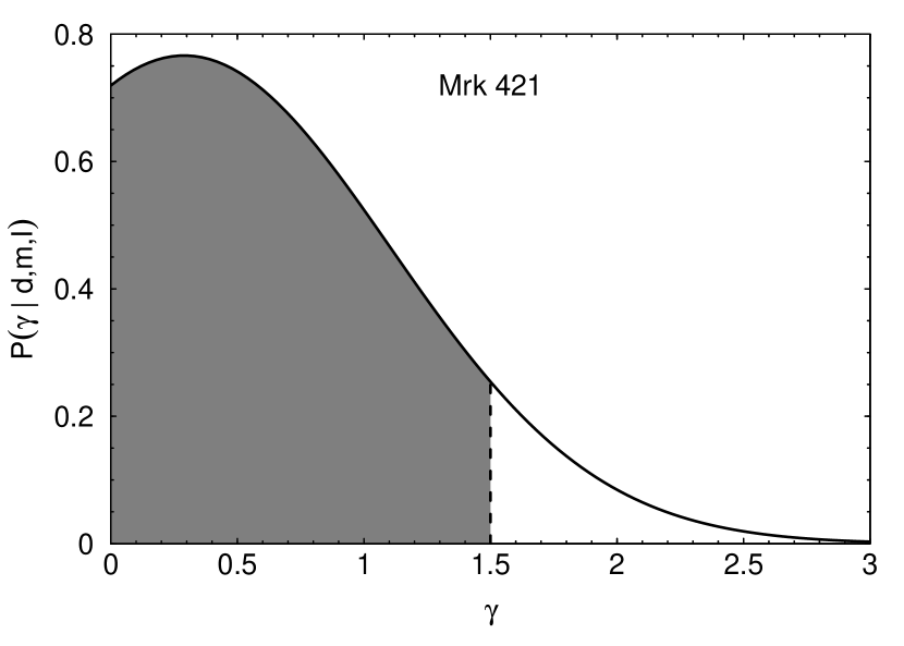
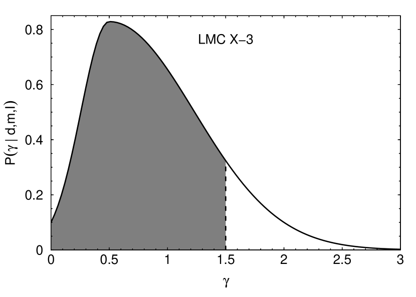
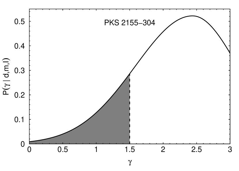
Figure 1.— Posterior probability distributions for $\gamma$, calculated from the observations in Table 2.1 using Equation (14). The shading indicates the region where $\gamma<3/2$, indicating that the hot halo is convectively unstable (Equation (8)).

In each panel of Figure 1 we have shaded the region where $\gamma<3/2$ – the area of this region gives us the probability that the hot halo is convectively unstable, under the assumption that the exponential halo models are accurate descriptions of the hot halo. These probabilities are shown in the final column of Table 2.1. On the Mrk 421 and LMC X-3 sight lines, there is a slightly less than 90% chance that the hot halo is convectively unstable. On the PKS 2155$-$304 sight line, however, the probability of convective instability is much lower.

4. EXTENDED HOT HALO MODELS

Typically, observational analyses that have concluded that the Milky Way’s hot halo is extended have assumed that the halo plasma is isothermal (Gupta et al., 2012, 2013; Miller & Bregman, 2013). While Gupta et al. (2012, 2013) assumed that the halo is of uniform density, in Miller & Bregman’s (2013) halo model the density decreases with Galactocentric distance (see Equation (3)), in which case the halo plasma will be convectively stable.

Fang et al. (2013) examined several different models for the hot halo. They found that both an exponential disk model (of the type discussed in the previous section) and a more extended non-isothermal halo in hydrostatic equilibrium with the Galaxy’s dark matter halo (Maller & Bullock, 2004) could be made consistent with the existing X-ray emission and pulsar dispersion measure data. Fang et al. (2013) argued that indirect evidence (the lack of gas in dwarf satellite galaxies and the possible pressure-confinement of high-velocity clouds) favored the extended Maller & Bullock-like halo (which Fang et al. refer to as the MB model).

The extended MB halo consists of adiabatic gas, with a polytropic index of 5/3. This means that the gas is isentropic, placing it on the boundary between convective stability and instability. However, in the absence of additional energy injection, radiative cooling would cause the entropy of Fang et al.’s (2013) MB model halo to change in such a way as to make the halo convectively unstable, as we will now show.

The change in the specific entropy, $d\mathcal{S}$, due to a radiative loss of energy $dQ$ is $d\mathcal{S}=-dQ/T$. In time $dt$, the energy lost to radiative cooling is $n^{2}\Lambda(T)dt$ per unit volume, or $(n/\bar{m})\Lambda(T)dt$ per unit mass, where $\Lambda(T)$ is the cooling function (e.g., Sutherland & Dopita, 1993), and $\bar{m}\approx 1\times 10^{-24}~{}\mbox{g}$ is the average mass per particle. Hence,

$$\frac{d\mathcal{S}}{dt}=-\frac{n\Lambda(T)}{\bar{m}T}.$$ (16)

Using the density and temperature profiles described by Fang et al.’s (2013) Equations (1) and (2), normalized such that $n=10^{-3.5}~{}\mbox{cm}^{-3}$ and $T=3.5\times 10^{6}~{}\mbox{K}$ at $r=1~{}\mbox{kpc}$ (Fang et al., 2013, Figure 1), we plot $d\mathcal{S}/dt$ as a function of Galactocentric radius in Figure 2.

Figure 2.— Rate of change of halo entropy due to radiative cooling as a function of Galactocentric distance, for Fang et al.’s (2013) MB halo model (calculated using Equation (16)).

Figure 2 shows that radiative cooling decreases the entropy of the MB model halo more rapidly at larger radii, out to $r\sim 70~{}\mbox{kpc}$. Hence, while the model halo is assumed to be isentropic, Figure 2 implies that this situation would not persist – radiative cooling would result in the entropy decreasing with $r$, and the halo would become convectively unstable. However, it should be noted that this change would occur slowly – the cooling time,

$$t_{\mathrm{cool}}=\frac{3kT}{2n\Lambda(T)},$$ (17)

of the MB model plasma is $\sim$1–2 Gyr. In addition, radiative cooling would change both the density and temperature structure of the halo – a detailed simulation would be required to check if the assumed density and temperature structure of the MB model halo would indeed ultimately give rise to convection.

5. DISCUSSION

5.1. The Observed Values of $\gamma$

When considering the exponential halo model (Section 3), we used published values of $\gamma$ that were derived from X-ray data alone. Yao et al. (2009) also investigated including FUSE O VI absorption line data in their analysis of the LMC X-3 sight line. They found that it tightened the constraint on $\gamma$, from $0.5^{+1.2}_{-0.4}$ to $0.8^{+0.3}_{-0.4}$. This appears to strengthen the conclusion that the halo is convectively unstable in this direction. However, for the following reasons, we excluded O VI from our analysis. In these exponential models, the O VI would reside several kiloparsecs above the disk. This contradicts the observation that $\sim$1/5 to $\sim$1/4 of the O VI column density originates below $|z|=1$ kpc (Bowen et al., 2008). In addition, Hagihara et al. (2010) point out that, because O VI-emitting plasma has a high cooling rate, it may be difficult to maintain an O VI-rich plasma high above the disk (although a detailed calculation would be needed to determine the extent to which this is true). Therefore, while including the O VI absorption data can apparently tighten the constraint on $\gamma$, this constraint may be unreliable.

The published values of $\gamma$ depend in part on the separation of the halo X-ray emission from the other components of the soft X-ray background (SXRB), namely, the foreground emission from the Local Bubble and/or from solar wind charge exchange, and the extragalactic background emission. For the PKS 2155$-$304 sight line, Hagihara et al. (2010) examined the effect of varying the normalization of the foreground component of their SXRB emission model – they tried both a normalization of zero, and a normalization $\sim$75% larger than their standard value. Decreasing (increasing) the foreground normalization decreased (increased) the halo temperature inferred from the emission spectrum, $T_{\mathrm{emis}}$ (Hagihara et al., 2010, Table 4).

The lower value of $T_{\mathrm{emis}}$ resulting from a foreground normalization of zero is consistent with $T_{\mathrm{abs}}$ for this sight line, implying that the halo is isothermal on this sight line. Indeed, with a foreground normalization of zero, the exponential halo model yields a relatively large value of $\gamma$ (3.39, versus 2.44 for their standard foreground model). The temperature scale height being a few times the density scale height implies that, from the point of view of the plasma relevant to X-ray observations, the halo is close to being isothermal. Since the density decreases with height, the halo is likely to be convectively stable in this case: with a foreground normalization of zero, Hagihara et al.’s (2010) results imply $P(\gamma<3/2)=0.05$, compared with 0.15 for their standard foreground normalization (Table 2.1). It should be noted, however, that a foreground normalization of zero may be unrealistic – models of solar wind charge exchange emission suggest that $\gtrsim$1 photons $\mbox{cm}^{-2}$ $\mbox{s}^{-1}$ $\mbox{sr}^{-1}$ of foreground O VII emission is present in most observed SXRB spectra (Koutroumpa et al., 2007), while Suzaku observations of the SXRB suggest a uniform foreground O VII intensity of $\sim$2 photons $\mbox{cm}^{-2}$ $\mbox{s}^{-1}$ $\mbox{sr}^{-1}$ (Yoshino et al. 2009; note that Hagihara et al. (2010) chose their standard foreground normalization to yield an O VII intensity of 2 photons $\mbox{cm}^{-2}$ $\mbox{s}^{-1}$ $\mbox{sr}^{-1}$).

At the other extreme, increasing Hagihara et al.’s (2010) foreground normalization led to a greater discrepancy between $T_{\mathrm{emis}}$ and $T_{\mathrm{abs}}$. This led to a smaller best-fit value of $\gamma$ (1.47), and to an increased probability of convective instability: $P(\gamma<3/2)=0.69$

Yao et al. (2009) also examined variants of their standard SXRB spectral model for the LMC X-3 sight line. They varied the normalization of the foreground component and the spectrum of the extragalactic component, and found that $\gamma$ was not strongly affected. However, these variations on Yao et al.’s (2009) analysis all included the O VI absorption data. It is unclear how sensitive the value of $\gamma$ derived for the LMC X-3 sight line from X-ray data alone would be to the other components of the SXRB. However, since $\gamma$ is better constrained for the LMC X-3 sight line than for the PKS 2155$-$304 sight line (compare rows 3 and 4 of Table 2.1), varying the other components of the SXRB model is unlikely to have as large an effect on $P(\gamma<3/2)$ for the LMC X-3 sight line as it did above for the PKS 2155$-$304 sight line.

In summary, we acknowledge that the uncertainty in the foreground component of the SXRB emission model introduces some uncertainty in our estimates of $P(\gamma<3/2)$ for the exponential halo model. However, there is insufficient information in the published studies that we have used to quantify this uncertainty.

The observed values of $\gamma$, and hence the probabilities of the halo being convectively unstable that we have calculated for the exponential halo model, may be refined in the light of future observations. In addition, future spectral analyses could use a Markov Chain Monte Carlo method (e.g., Press et al., 2007, Section 15.8) to explore the model parameter space. Using such a method would allow one to obtain the posterior distribution for $\gamma$ directly from the spectral analysis, rather than having to infer it from the confidence intervals derived by varying $\chi^{2}$. Furthermore, such an approach could allow one to marginalize over the normalization of the foreground component of the SXRB emission model. This means that the posterior distribution for $\gamma$ (and hence the probability of convective instability) would automatically take into account the uncertainty in the foreground emission.

5.2. Implications for the Hot Halo

The observational results based on the exponential halo model imply that the probability that the halo is convectively unstable in the direction of PKS 2155$-$304 is much lower than in the directions of LMC X-3 or Mrk 421 (Table 2.1). Since the halo is observed to be non-uniform in emission (e.g., Yoshino et al., 2009; Henley et al., 2010; Henley & Shelton, 2013), it is entirely possible for some regions of the hot halo to be convectively unstable and for others to be stable. Note that PKS 2155$-$304 is 73° and 164° from LMC X-3 and Mrk 421, respectively, and so the regions of the halo that these sight lines are probing are well separated.

For a given halo model, we can using Equation (17) to calculate the cooling time of the halo gas as a function of height, $z$, or Galactocentric radius, $r$. We can then use $z/t_{\mathrm{cool}}(z)$ or $r/t_{\mathrm{cool}}(r)$ to estimate the speed at which the halo fluid must convect upward in order to offset the radiative losses. We can compare this with the adiabatic sound speed,

$$v_{\mathrm{sound}}=\sqrt{\frac{5kT}{3\bar{m}}},$$ (18)

to see if the radiative energy losses can be offset by subsonic convective heating.

Figure 3.— The ratio of the estimated speed at which the halo fluid must convect upward in order to offset the radiative losses, $z/t_{\mathrm{cool}}$ or $r/t_{\mathrm{cool}}$, to the adiabatic sound speed, $v_{\mathrm{sound}}$. This ratio was calculated using Equations (17) and (18). The solid and dashed curves were calculated using the best-fit exponential halo models for the Mrk 421 and LMC X-3 sight lines, respectively (Sakai et al., 2012; Yao et al., 2009), and are plotted as functions of height, $z$. The dotted curve was calculated using Fang et al.’s (2013) MB model, and is plotted as a function of Galactocentric distance, $r$. The horizontal dot-dash line indicates $z/t_{\mathrm{cool}}$ or $r/t_{\mathrm{cool}}=v_{\mathrm{sound}}$.

Figure 3 shows $(z/t_{\mathrm{cool}})/v_{\mathrm{sound}}$ as a function of $z$, calculated using the best-fit exponential halo models for the Mrk 421 (solid) and LMC X-3 (dashed) sight lines (Sakai et al., 2012; Yao et al., 2009). Up to $z\sim 2.5~{}\mbox{kpc}$, $(z/t_{\mathrm{cool}})/v_{\mathrm{sound}}<1$. Since these models imply that most of the X-ray-emitting and O VII- and O VIII-bearing gas resides below $\sim$2.5 kpc (at which height $T\sim 6\times 10^{5}~{}\mbox{K}$; Yao et al. 2009; Sakai et al. 2012), this result implies that this region could be kept hot by subsonic convection replacing cooling gas with hotter gas from below.

Figure 3 also shows $(r/t_{\mathrm{cool}})/v_{\mathrm{sound}}$ for the MB model discussed in Section 4 (Fang et al., 2013). For this model, $(r/t_{\mathrm{cool}})/v_{\mathrm{sound}}<1$ out to a Galactocentric distance of at least 100 kpc. The main reason $(r/t_{\mathrm{cool}})/v_{\mathrm{sound}}$ is small for this model is that the cooling time is long, as noted in Section 4. Hence, if radiative cooling perturbed the MB model, resulting in a convective instability (Section 4), subsonic convection should be able to maintain the temperature of the halo, in spite of radiative losses.

When considering the exponential models of the halo, we reiterate the point made in Section 3.3 that the probabilities that the halo is convectively unstable (Table 2.1) are conditional upon these exponential models being good descriptions of the hot halo. We noted in Section 2.3 that, in reality, the halo may consist of an exponential-like distribution in the lower halo, plus a more extended, low-density halo suggested by indirect evidence and expected from disk galaxy formation simulations. We do not attempt to come up with a composite halo model here, but point out that the instability criterion derived in Section 3.1 may be applied to the exponential portion of such a model.

Another issue that we do not attempt to address is the timescale on which convection would tend to change the density and temperature distributions of the model halos we have examined. Could a dynamical equilibrium exist, or would convection tend to smooth out the temperature distribution on a short timescale? If this timescale is short, it may argue against certain convectively unstable models being accurate descriptions of the hot halo gas. Alternatively, one could require that a model halo be convectively stable. In the case of the exponential halo model, this would involve imposing a lower limit of 3/2 on $\gamma$ in the spectral analysis. More generally, it would involve requiring that a model halo’s entropy, $Tn^{-2/3}$, increases with distance from the Galaxy. If, on the other hand, convectively unstable halo models are good descriptions of the hot halo gas, in the lower halo at least, this argues in favor of this gas being heated from the bottom, by supernova activity in the disk.

6. SUMMARY

We have examined the convective stability of the Milky Way’s hot halo. Halo models in which the density and temperature decrease exponentially with height (Yao & Wang, 2007; Yao et al., 2009; Hagihara et al., 2010; Sakai et al., 2012) are convectively unstable if $\gamma<3/2$, where $\gamma$ is the ratio of the temperature and density scale heights (Section 3.1). Using the published best-fit values and confidence intervals for $\gamma$, derived from joint analyses of X-ray emission and absorption line data (Section 3.2), we calculated the posterior probabilities for the hot halo being convectively unstable, under the assumption that these exponential models are good descriptions of the halo (Section 3.3). We found that these probabilities are just under 90% in the directions of LMC X-3 and Mrk 421 (Yao et al., 2009; Sakai et al., 2012), but only 15% in the direction of PKS2155$-$304 (Hagihara et al., 2010). These results imply that, if the published exponential models are good descriptions of the hot gas distribution (at least in the lower halo), this gas is reasonably likely to be convectively unstable in two out of three directions, arguing in favor of it being heated from the bottom by supernova activity in the disk.

We also examined model distributions in which the hot halo gas is more extended (Section 4). A variety of such models exists. Miller & Bregman (2013) assumed an isothermal halo in which the gas density is described by a $\beta$-model in their analysis of O VII absorption line data. This model halo is convectively stable, as the temperature of the gas is constant while its density decreases with distance from the Galaxy. Fang et al. (2013), meanwhile, showed that a model in which the hot halo is assumed to be a non-isothermal gas in hydrostatic equilibrium with the Galaxy’s dark matter (Maller & Bullock, 2004) is consistent with the existing pulsar dispersion measure and X-ray emission data. The gas in this model is isentropic, and would thus be on the border between convective stability and instability if radiative cooling were unimportant. However, we found that radiative cooling could perturb this model toward instability, and hence that heating from disk supernovae via convection could play a role in maintaining such a halo against radiative heat loss.

References

- Avillez & Mac Low (2001) Avillez, M. A., & Mac Low, M.-M. 2001, ApJ, 551, L57
- Avni (1976) Avni, Y. 1976, ApJ, 210, 642
- Bowen et al. (2008) Bowen, D. V., Jenkins, E. B., Tripp, T. M., et al. 2008, ApJS, 176, 59
- Bregman (1980) Bregman, J. N. 1980, ApJ, 236, 577
- Crain et al. (2010) Crain, R. A., McCarthy, I. G., Frenk, C. S., Theuns, T., & Schaye, J. 2010, MNRAS, 407, 1403
- Fang et al. (2013) Fang, T., Bullock, J., & Boylan-Kolchin, M. 2013, ApJ, 762, 20
- Gupta et al. (2009) Gupta, A., Galeazzi, M., Koutroumpa, D., Smith, R., & Lallement, R. 2009, ApJ, 707, 644
- Gupta et al. (2013) Gupta, A., Mathur, S., Galeazzi, M., & Krongold, Y. 2013, ApJ, submitted (arXiv:1307.6195)
- Gupta et al. (2012) Gupta, A., Mathur, S., Krongold, Y., Nicastro, F., & Galeazzi, M. 2012, ApJ, 756, L8
- Hagihara et al. (2010) Hagihara, T., Yao, Y., Yamasaki, N. Y., et al. 2010, PASJ, 62, 723
- Henley & Shelton (2008) Henley, D. B., & Shelton, R. L. 2008, ApJ, 676, 335
- Henley & Shelton (2013) Henley, D. B., & Shelton, R. L. 2013, ApJ, 773, 92
- Henley et al. (2010) Henley, D. B., Shelton, R. L., Kwak, K., Joung, M. R., & Mac Low, M.-M. 2010, ApJ, 723, 935
- Hill et al. (2012) Hill, A. S., Joung, M. R., Mac Low, M.-M., et al. 2012, ApJ, 750, 104
- Joung & Mac Low (2006) Joung, M. K. R., & Mac Low, M.-M. 2006, ApJ, 653, 1266
- Koutroumpa et al. (2007) Koutroumpa, D., Acero, F., Lallement, R., Ballet, J., & Kharchenko, V. 2007, A&A, 475, 901
- Koutroumpa et al. (2011) Koutroumpa, D., Smith, R. K., Edgar, R. J., et al. 2011, ApJ, 726, 91
- Kuntz & Snowden (2000) Kuntz, K. D., & Snowden, S. L. 2000, ApJ, 543, 195
- Lampton et al. (1976) Lampton, M., Margon, B., & Bowyer, S. 1976, ApJ, 208, 177
- Mac Low et al. (1989) Mac Low, M.-M., McCray, R., & Norman, M. L. 1989, ApJ, 337, 141
- Maller & Bullock (2004) Maller, A. H., & Bullock, J. S. 2004, MNRAS, 355, 694
- McCammon et al. (2002) McCammon, D., Almy, R., Apodaca, E., et al. 2002, ApJ, 576, 188
- Miller & Bregman (2013) Miller, M. J., & Bregman, J. N. 2013, ApJ, 770, 118
- Nicastro et al. (2002) Nicastro, F., Zezas, A., Drake, J., et al. 2002, ApJ, 573, 157
- Norman & Ikeuchi (1989) Norman, C. A., & Ikeuchi, S. 1989, ApJ, 345, 372
- Press et al. (2007) Press, W. H., Teukolsky, S. A., Vetterling, W. T., & Flannery, B. P. 2007, Numerical Recipes – The Art of Scientific Computing, 3rd edn. (Cambridge: Cambridge University Press)
- Rasmussen et al. (2003) Rasmussen, A., Kahn, S. M., & Paerels, F. 2003, in The IGM/Galaxy Connection. The Distribution of Baryons at , ed. J. L. Rosenberg & M. E. Putman (Dordrecht: Kluwer), 109
- Rasmussen et al. (2009) Rasmussen, J., Sommer-Larsen, J., Pedersen, K., et al. 2009, ApJ, 697, 79
- Sakai et al. (2012) Sakai, K., Mitsuda, K., Yamasaki, N. Y., et al. 2012, in AIP Conf. Proc. 1427, SUZAKU 2011: Exploring the X-ray Universe: Suzaku and Beyond, ed. R. Petre, K. Mitsuda, & L. Angelini (Melville: AIP), 342
- Shapiro & Field (1976) Shapiro, P. R., & Field, G. B. 1976, ApJ, 205, 762
- Shu (1992) Shu, F. H. 1992, The Physics of Astrophysics, Volume II: Gas Dynamics (Sausalito, CA: University Science Books)
- Sivia & Skilling (2006) Sivia, D. S., & Skilling, J. 2006, Data Analysis: A Bayesian Tutorial, 2nd edn. (Oxford: Oxford University Press)
- Smith et al. (2007) Smith, R. K., Bautz, M. W., Edgar, R. J., et al. 2007, PASJ, 59, S141
- Sutherland & Dopita (1993) Sutherland, R. S., & Dopita, M. A. 1993, ApJS, 88, 253
- Toft et al. (2002) Toft, S., Rasmussen, J., Sommer-Larsen, J., & Pedersen, K. 2002, MNRAS, 335, 799
- Wang & Yao (2012) Wang, Q. D., & Yao, Y. 2012, arXiv:1211.4834
- Yao & Wang (2007) Yao, Y., & Wang, Q. D. 2007, ApJ, 658, 1088
- Yao et al. (2009) Yao, Y., Wang, Q. D., Hagihara, T., et al. 2009, ApJ, 690, 143
- Yoshino et al. (2009) Yoshino, T., Mitsuda, K., Yamasaki, N. Y., et al. 2009, PASJ, 61, 805