Stochastic Interactions of Two Brownian Hard Spheres in the Presence of Depletants

Abstract

A quantitative analysis is presented for the stochastic interactions of a pair of Brownian hard spheres in non-adsorbing polymer solutions. The hard spheres are hypothetically trapped by optical tweezers and allowed for random motion near the trapped positions. The investigation focuses on the long-time correlated Brownian motion. The mobility tensor altered by the polymer depletion effect is computed by the boundary integral method, and the corresponding random displacement is determined by the fluctuation-dissipation theorem. From our computations it follows that the presence of depletion layers around the hard spheres has a significant effect on the hydrodynamic interactions and particle dynamics as compared to pure solvent and pure polymer solution (no depletion) cases. The probability distribution functions of random walks of the two interacting hard spheres that are trapped clearly shifts due to the polymer depletion effect. The results show that the reduction of the viscosity in the depletion layers around the spheres and the entropic force due to the overlapping of depletion zones have a significant influence on the correlated Brownian interactions.

I Introduction

The interactions between dispersed colloidal particles in solutions containing non-adsorbing polymer chains play an essential role in many phenomena and processes including macromolecular crowding, protein crystallization, food processing, and co- and self-assembly zimmerman1993macromolecular ; ellis2003join ; doublier2000protein ; tanaka2002protein ; rossi2011cubic . Adding non-adsorbing polymer chains to a dispersion of colloids effectively induces an attractive potential between the colloidal particles asakura1954interaction ; asakura1958interaction ; vrij1976polymers and alters their phase behavior gast1983polymer ; lekkerkerker1992phase ; lekkerkerker1994phase ; poon2002physics ; koda2002test ; fleer2008analytical and transport properties tuinier2006depletion . These changes originate from the presence of polymer depletion zones around the colloidal particles. To avoid the reduction of conformation entropy, polymers prefer to stay away from the colloidal surfaces. Hence depletion zones appear around the colloidal particles. Within the depletion zone the polymer concentration is reduced significantly compared to the bulk polymer concentration. The overlap of depletion layers causes an unbalanced osmotic pressure distribution by the polymers around the colloids, first understood by Asakura and Oosawa asakura1954interaction ; asakura1958interaction . The resulting attractive potential’s range and depth can be tuned by polymer size, concentration, and solution conditions. In the last few decades many studies on polymer depletion were focused on the equilibrium aspects of colloid-polymer mixtures, primarily on the depletion interaction, phase behaviors, microstructure of the colloid-polymer suspensions, and scattering properties gast1983polymer ; lekkerkerker1992phase ; verma1998entropic ; fuchs2002structure ; poon2002physics ; koda2002test ; dzubiella2002phase ; mutch2007colloid ; kleshchanok2008direct .

In order to quantify the dynamic effects of a depletion layer, Donath and coworkers proposed an approximation for the hydrodynamic friction of a sphere in a non-adsorbing polymer solution by considering a slip boundary condition at the surface of the particle donath1997stokes . Tuinier and Taniguchi considered a viscosity profile near the surface that followed polymer segment density profile and could account for the polymer depletion-induced flow behavior close to a flat interface tuinier2005polymer . The translational and rotational motion of a sphere and a pair of spheres through a non-adsorbing polymer were investigated by Fan et. al. tuinier2006depletion ; fan2007motion ; fan2007asymptotic ; fan2010hydrodynamic using both a simplified two-layer model tuinier2006depletion ; fan2007motion and a continuous viscous profile fan2007asymptotic ; fan2010hydrodynamic . For the continuous case, the equilibrium distribution of polymers was determined by mean-field theory fleer2003mean . When two colloidal spheres are suspended in a liquid, they transfer momentum to each other by the hydrodynamic interactions and hence their stochastic motion is correlated. A popular way to directly measure the interactions between colloidal particles is to hold the particles in a desired separation distance which can be done by applying an optical trap, first introduced by Ashkin et. al. ashkin1986observation . This optical tweezer method has been used to measure the pair interactions under charge stabilization crocker1994microscopic and the attractive entropic effect verma1998entropic ; verma2000attractions . Crocker crocker1997measurement developed a blinking optical trap to measure the free diffusive motion of pair particles. Two spherical particles were brought into a desired separation distance when the tweezer is on, while particles start to diffuse freely when off. The cross-correlation analysis of hydrodynamic interactions of two particles was studied experimentally using optical tweezers meiners1999direct ; bartlett2001measurement ; reichert2004hydrodynamic . The method has been extended to investigate the dynamics of optically bounded particles metzger2007measurement and the shear effect ziehl2009direct ; bammert2010dynamics .

Hence there is a strong need in theoretically quantifying the polymer depletion effect on the stochastic interactions of a pair of colloidal particles. Here we present the results of the mobility functions of two interacting spheres and the thermodynamic potential due to the entropic effect. The self- and cross-correlation of the pair particles’ random displacements under dilute to semi-dilute polymer solution conditions are compared to pure solvent case. When accounting for polymer, the polymer entanglement is neglected and the fluid flow is assumed Newtonian. Background polymer fluctuations are also not considered here. The simplified two-layer continuum model is applied to both hydrodynamic and thermodynamic interactions. The polymer structure relaxation is assumed much faster than the long-time Brownian motion such that the depletion envelop always follows the sphere’s trajectory. The mobility is computed deterministically by the boundary integral method, and the result is coupled to the random displacements of the colloidal hard spheres to ensure the consistency of the fluctuation-dissipation theorem.

II Theoretical Formulation

We consider Brownian motion of a pair of isotropic and equal-sized hard spheres in a dilute to semi-dilute non-adsorbing polymer solution. It is assumed that each colloidal particle is surrounded by an assumed equilibrium depletion layer. The mean positions of both hard spheres are fixed by the optical traps as illustrated in Fig. 1. The depletion zone around each sphere is represented by the simplified two-layer model tuinier2006depletion that has uniform solvent viscosity ($\eta_{\textrm{s}}$) in the inner layer ($\Omega_{\textrm{s}}$) and uniform bulk polymer solution viscosity ($\eta_{\textrm{p}}$) in the bulk ($\Omega_{\textrm{p}}$).

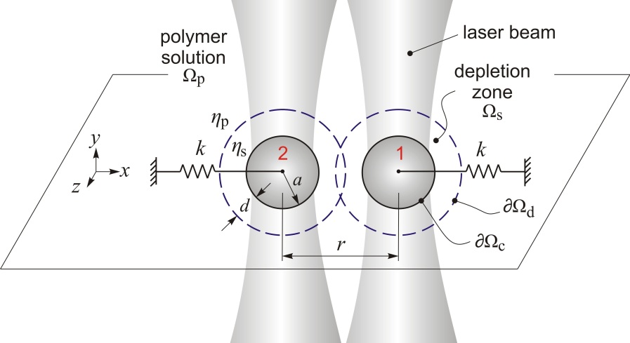
Figure 1: Schematic of a pair of interacting colloidal spheres located by optical tweezers. The domains $\Omega_{\textrm{p}}$ and $\Omega_{\textrm{s}}$ are for the bulk solution and the polymer depletion zones, respectively. $\eta_{\textrm{p}}$ and $\eta_{\textrm{s}}$ are the corresponding bulk and solvent viscosities. The distance $d$ is the apparent thickness of the depletion layer, $a$ is colloid radius, and $k$ is the stiffness that represents the trapping potential. The particle tags 1 and 2 are given.

II.1 Two-Layer Model

In the bulk, the polymer solution viscosity can be approximated by the Martin equation rodriguez1973graphical :

$$\lambda=\frac{\eta_{\textrm{p}}}{\eta_{\textrm{s}}}=1+[\eta]c_{\textrm{b}}e^{k_{\textrm{H}}[\eta]c_{\textrm{b}}}=1+\epsilon e^{k_{\textrm{H}}\epsilon},$$ (1)

where $\eta_{\textrm{p}}$ and $\eta_{\textrm{s}}$ are the corresponding bulk and solvent viscosities, respectively, $c_{\textrm{b}}$ is the bulk polymer concentration, $[\eta]=1/c^{*}_{\textrm{b}}$ is the intrinsic viscosity of the polymer, $c^{*}_{\textrm{b}}$ is the polymer overlap concentration, and $k_{\textrm{H}}$ is the Huggins coefficient. For the polymer concentration we use the scaled quantity $\epsilon=[\eta]c_{\textrm{b}}=c_{\textrm{b}}/c^{*}_{\textrm{b}}$.

The depletion thickness around the hard spheres can be calculated based on the bulk concentration and the sizes of the polymers and colloid spheres. As a correction of the depletion thickness at a planar surface $d_{\textrm{P}}$ fleer2003mean , the thickness at a spherical surface can be expressed as

$$d=a\left[{1+3\frac{d_{\textrm{P}}}{a}+\frac{\pi^{2}}{4}\left(\frac{d_{\textrm{P}}}{a}\right)^{2}}\right]^{1/3}-a,$$ (2)

where $d_{\textrm{P}}$ is the depletion thickness for a planar surface, $a$ is the colloid radius, $d_{\textrm{P}}=d_{0}\sqrt{1/(1+c_{1}\epsilon^{2})}$, where $d_{0}=2R_{g}/\sqrt{\pi}$ indicates the thickness in the dilute limit, and $R_{g}$ is the radius of gyration of polymers. The coefficient $c_{1}$ is around $6.02$ for polymers in a theta solvent fleer2003mean ; fleer2008analytical .

According to the Asakara-Oosawa-Vrij (AOV) model  asakura1954interaction ; vrij1976polymers , the depletion potential between two hard spheres in a solution of dilute depletants is given by the product of the osmotic pressure $\Pi$ and the overlap volume of the polymer depletion zones vrij1976polymers :

$$W^{\textrm{dep}}(\epsilon,r)=\begin{cases}\displaystyle\infty~{}~{}\textrm{for}~{}~{}r\leq 2a\\ \displaystyle{-\frac{4\pi}{3}(a+d)^{3}\left[1-\frac{3}{4}\left(\frac{r}{a+d}\right)+\frac{1}{16}\left(\frac{r}{a+d}\right)^{3}\right]\Pi(\epsilon)}\\ ~{}~{}~{}~{}~{}~{}~{}~{}~{}~{}~{}~{}\textrm{for}~{}~{}2a<r\leq 2(a+d)\\ 0\quad\textrm{for}\quad r>2(a+d),\end{cases}$$ (3)

where $r=|\mathbf{r}_{1}-\mathbf{r}_{2}|$ is the center-to-center distance of the hard spheres, $\Pi(\epsilon)=\Pi_{0}[1+c_{2}\epsilon^{2}]$ approximates the osmotic pressure in the dilute to semi-dilute regime fleer2008analytical , where $\Pi_{0}(\epsilon)=n_{\textrm{b}}(\epsilon)k_{\textrm{B}}T$ is the for dilute limit with $n_{\textrm{b}}(\epsilon)=3\epsilon/(4\pi R_{g}^{3})$ as the number density of polymers, and $c_{2}$ is around $4.1$ for a theta solvetnt fleer2008analytical . The corresponding depletion force therefore is

$$\mathbf{F}^{\textrm{dep}}_{\alpha}(\epsilon,r)=-\nabla W^{\textrm{dep}}(\epsilon,r)$$ (4)

$$\quad\quad\quad={\pi}(a+d)^{2}\left[1-\frac{1}{4}\left(\frac{r}{a+d}\right)^{2}\right]\Pi(\epsilon)~{}\mathbf{\hat{r}}_{\alpha\beta}$$

for $2a<r\leq 2(a+d)$, where $\mathbf{\hat{r}}_{\alpha\beta}=[\mathbf{r}_{\beta}-\mathbf{r}_{\alpha}]/r$ is the unit vector pointing from particle $\alpha$ to $\beta$.

II.2 Brownian Interactions

The translational Brownian motions of both spheres in two quiescent fluid can be described by the general Langevin equation deutch1971molecular :

$$m_{\alpha}\ddot{\mathbf{r}}_{\alpha}=\textbf{F}_{\alpha}^{\textrm{H}}+\textbf{F}_{\alpha}^{\textrm{P}}+\textbf{F}_{\alpha}^{\textrm{B}}~{}~{}~{}~{}~{}~{}(\alpha=1,2),$$ (5)

where $m$ is the particle mass, $\alpha$ labels particles 1 and 2, $\mathbf{r}$ is the particle position vector, and the force summation acting on the hard spheres includes contributions of hydrodynamic forces ($\textbf{F}_{\alpha}^{\textrm{H}}$), polymer depletion and optical trapping forces (non-hydrodynamic, $\textbf{F}_{\alpha}^{\textrm{P}}$), and the random thermal fluctuation force ($\textbf{F}_{\alpha}^{\textrm{B}}$) that drives the Brownian motion. They can be written as

$$\textbf{F}_{\alpha}^{\textrm{H}}=-\left(\bm{\zeta}_{\alpha 1}\cdot\dot{\mathbf{r}}_{1}+\bm{\zeta}_{\alpha 2}\cdot\dot{\mathbf{r}}_{2}\right),$$ (6)

$$\textbf{F}_{\alpha}^{\textrm{P}}=\textbf{F}_{\alpha}^{\textrm{dep}}+\textbf{F}_{\alpha}^{\textrm{trap}},$$ (7)

and

$$\textbf{F}_{\alpha}^{\textrm{B}}=\bm{\kappa}_{\alpha 1}\cdot\textbf{x}_{1}+\bm{\kappa}_{\alpha 2}\cdot\textbf{x}_{2},$$ (8)

where $\bm{\zeta}$ is the resistance tensor, $\bm{\kappa}$ is the weighting coefficient tensor and the vector x contains random numbers in Cartesian coordinates and is defined by a Gaussian distribution with mean $\langle\textbf{x}_{\alpha}(t)\rangle=\textbf{0}$ and co-variance $\langle\textbf{x}_{\alpha}(t)\textbf{x}_{\beta}(t+t^{\prime})\rangle=2\delta_{\alpha\beta}\delta(t^{\prime})\textbf{I}$, where $\delta$ is the Kronecker delta, I is the identity tensor, and $\alpha,\beta$=1, 2. The coefficient $\bm{\kappa}$ is related to the thermal energy $k_{\textrm{B}}T$ and the resistance tensor $\bm{\zeta}$ through the fluctuation-dissipation theory kubo1966fluctuation ,

$$\bm{\zeta}_{\alpha\beta}=\frac{1}{k_{\textrm{B}}T}\left(\bm{\kappa}_{\alpha 1}\cdot\bm{\kappa}_{1\beta}+\bm{\kappa}_{\alpha 2}\cdot\bm{\kappa}_{2\beta}\right)~{}~{}~{}~{}~{}~{}(\alpha,\beta=1,2).$$ (9)

The non-hydrodynamic force includes the entropic and optical trapping forces. For a small displacement away from the equilibrium position of the hard spheres, the optical trap provides a three-dimensional harmonic force Tlusty1998 :

$$\mathbf{F}^{\textrm{trap}}_{\alpha}=-k\left[\mathbf{r}_{\alpha}(t)-\mathbf{r}_{\alpha}^{0}\right],$$ (10)

where $k$ is the apparent stiffness of the potential, and the superscript 0 indicates the equilibrium position in absence of the depletion potential. The stiffness of the harmonic force is approximately a linear function of the light intensity Tlusty1998 .

In order to quantify typical time scales we consider colloidal spheres with radius 500 nm in an optical trap with a stiffness of 18.5 pN$/\mu$m meiners1999direct in an aqueous solvent. The characteristic relaxation time for the colloidal Brownian motion under the potential can then be estimated by $6\pi\eta_{\textrm{s}}a/k\simeq 10^{-3}$ s. If the mass density of the colloid is similar to solvent, the momentum relaxation or decorrelation time, $m/6\pi\eta_{\textrm{s}}a$, is about $10^{-7}$ s, where $\eta_{\textrm{s}}$ is the solvent viscosity. The diffusive time scale for the colloid over its radius is $\sim{6\pi\eta_{\textrm{s}}a^{3}}/{k_{\textrm{B}}T}\simeq 0.6$ s. Therefore for the long-time diffusive interaction, the motion of hard spheres is overdamped and the inertial effect is assumed negligible. By integrating the quasi-steady Langevin equation the new position for the colloidal sphere $\alpha$ at each simulation time step ($\gg$ momentum decorrelation time) can be described by the following diffusive displacement equation ermak1978brownian :

$$\mathbf{r}_{\alpha}(t+\Delta t)= \mathbf{r}_{\alpha}(t)+\left[\frac{\partial}{\partial\mathbf{r}_{1}(t)}\cdot\mathbf{D}_{\alpha 1}(t)+\frac{\partial}{\partial\mathbf{r}_{2}(t)}\cdot\mathbf{D}_{\alpha 2}(t)\right]\Delta t$$

$$~{}~{}+\frac{1}{k_{\textrm{B}}T}\left[\mathbf{D}_{\alpha 1}(t)\cdot\textbf{F}_{1}^{P}(t)+\mathbf{D}_{\alpha 2}(t)\cdot\textbf{F}_{2}^{P}(t)\right]\Delta t+\mathbf{R}_{\alpha}(\Delta t),~{}~{}$$

where $\mathbf{D}_{\alpha\beta}$ ($\alpha,\beta$=1,2) is the diffusion tensor, $\Delta t$ is the integration time step, and $\mathbf{R}_{\alpha}$ is the random displacement that has zero mean $\langle\textbf{R}_{\alpha}(\Delta t)\rangle=\textbf{0}$, and covariance $\langle\mathbf{R}_{\alpha}(\Delta t)\mathbf{R}_{\beta}(\Delta t)\rangle=2\mathbf{D}_{\alpha\beta}(t)\Delta t$. The displacements resulting from the spatial variation of the diffusion tensor, the potential forces acting on both hard spheres, and the thermal fluctuation are all included in the formulation. Computationally, the random displacement vector can be determined by $R_{i}(\Delta t)=\sum_{j=1}^{i}L_{\emph{ij}}(\mathbf{D}_{\alpha\beta})X_{\emph{j}}(\Delta t)$ ($i=1,2,...6$), where $i=1,2,3$ represent Cartesian components for colloid $\alpha=1$, and $i=4,5,6$ are components for colloid $\alpha=2$, tensor $L$ is the weighting factor for random displacement, $\mathbf{L}_{\alpha\beta}=\left(\mathbf{D}_{\alpha 1}\cdot\bm{\kappa}_{1\beta}+\mathbf{D}_{\alpha 2}\cdot\bm{\kappa}_{2\beta}\right)/{k_{\textrm{B}}T}$, and $X_{1},X_{2},...X_{6}$ are series of random variables with zero mean and a covariance of $\sqrt{2\Delta t}$ ermak1978brownian .

II.3 Mobility Functions

Since we apply the two layer approach to account for the depletion zones, the Rotne-Prager tensors rotne1969variational or higher-order corrections batchelor1976brownian are not applicable for resolving the self- and mutual-diffusivity. The diffusivity $\mathbf{D}_{\alpha\beta}=k_{\textrm{B}}T\bm{\zeta}_{\alpha\beta}^{-1}$ here is quantified based on the distance between the hard spheres ($r$), the thickness of polymer depletion layer ($d$), and the bulk-to-solvent viscosity ratio ($\lambda=\eta_{\textrm{p}}/\eta_{\textrm{s}}$). The self-diffusivity can be formulated as a correction of the mobility functions batchelor1976brownian ; dhont1996introduction for the motion of a pair of spheres in a homogeneous medium,

$$\mathbf{D}_{\alpha\alpha}(r,d,\lambda)=\frac{D_{0}}{g_{0}(d,\lambda)}\Big{[}\mathbf{I}+A^{\textrm{s}}(r,d,\lambda)\mathbf{\hat{r}}_{\alpha\beta}\mathbf{\hat{r}}_{\alpha\beta}+B^{\textrm{s}}(r,d,\lambda)\left(\mathbf{I}-\mathbf{\hat{r}}_{\alpha\beta}\mathbf{\hat{r}}_{\alpha\beta}\right)\Big{]},$$ (12)

where $\alpha,\beta=1,2$ and $\alpha\neq\beta$, $g_{0}(d,\lambda)$ is the correction factor for the hydrodynamic friction coefficient of an isolated hard sphere $6\pi\eta_{\textrm{s}}a$ due to the depletion layer fan2007motion , $D_{0}=k_{\textrm{B}}T/6\pi\eta_{\textrm{s}}a$ is the diffusivity of an isolated sphere in a pure solvent, $\mathbf{I}$ is the identity matrix, $A$ and $B$ are mobility functions in parallel and perpendicular directions, respectively, and the superscript s is for self-mobility. Throughout this paper the correction factor $g$ with any super- and sub-script describes the deviation of the friction from a single sphere in a pure solvent (for which $g=1$). Similarly, the mutual diffusivity can be expressed as

$$\mathbf{D}_{\alpha\beta}(r,d,\lambda)=\frac{D_{0}}{g_{0}(d,\lambda)}\Big{[}A^{\textrm{c}}(r,d,\lambda)\mathbf{\hat{r}}_{\alpha\beta}\mathbf{\hat{r}}_{\alpha\beta}+B^{\textrm{c}}(r,d,\lambda)\left(\mathbf{I}-\mathbf{\hat{r}}_{\alpha\beta}\mathbf{\hat{r}}_{\alpha\beta}\right)\Big{]},$$ (13)

where $\alpha,\beta=1,2$ and $\alpha\neq\beta$, the superscript c indicates cross-mobility. The analytical expression for a single particle based on the two-layer approximation is given by fan2007motion

$$g_{0}(d,\lambda)=\frac{2}{\Gamma}\left[\left(2+{3}{\lambda}^{-1}\right)\left(1+{d}^{*}\right)^{6}-2\left(1-{\lambda}^{-1}\right)\left(1+{d}^{*}\right)\right],$$ (14)

where $d^{*}=d/a$ is the normalized depletion thickness and

$$\Gamma= 2\left(2+{3}{\lambda}^{-1}\right)\left(1+{d}^{*}\right)^{6}-3\left(3+{2}{\lambda}^{-1}\right)\left(1-{\lambda}^{-1}\right)\left(1+{d}^{*}\right)^{5}$$

$$+10\left(1-{\lambda}^{-1}\right)\left(1+{d}^{*}\right)^{3}-9\left(1-{\lambda}^{-1}\right)\left(1+{d}^{*}\right)+4\left(1-{\lambda}^{-1}\right)^{2}.$$

Here the mobility functions are decoupled and computed by the boundary integral method. Specifically, the four functions are expressed as

$$\displaystyle{A^{\textrm{s}}(r,d,\lambda)=\frac{g_{0}(d,\lambda)}{2}\left[\frac{1}{g_{\|}^{\textrm{I}}(r,d,\lambda)}+\frac{1}{g_{\|}^{\textrm{II}}(r,d,\lambda)}\right]-1},~{}~{}~{}~{}~{}~{}$$ (16)

$$\displaystyle{B^{\textrm{s}}(r,d,\lambda)=\frac{g_{0}(d,\lambda)}{2}\left[\frac{1}{g_{\bot}^{\textrm{I}}(r,d,\lambda)}+\frac{1}{g_{\bot}^{\textrm{II}}(r,d,\lambda)}\right]-1},$$

$$\displaystyle{A^{\textrm{c}}(r,d,\lambda)=\frac{g_{0}(d,\lambda)}{2}\left[\frac{-1}{g_{\|}^{\textrm{I}}(r,d,\lambda)}+\frac{1}{g_{\|}^{\textrm{II}}(r,d,\lambda)}\right]},\quad\textrm{ and}$$

$$\displaystyle{B^{\textrm{c}}(r,d,\lambda)=\frac{g_{0}(d,\lambda)}{2}\left[\frac{-1}{g_{\bot}^{\textrm{I}}(r,d,\lambda)}+\frac{1}{g_{\bot}^{\textrm{II}}(r,d,\lambda)}\right]},$$

where $g_{\|}^{\textrm{I}}$, $g_{\|}^{\textrm{II}}$, $g_{\bot}^{\textrm{I}}$, and $g_{\bot}^{\textrm{II}}$ are the corrections or the scaled resistances due to depletion effect and the hydrodynamic interaction between both spheres, defined as

$$g_{\|}^{\textrm{I}}(r,d,\lambda)=\displaystyle\frac{F_{\|}^{\textrm{I}}(r,d,\lambda)}{6\pi\eta_{\textrm{s}}aU},~{}~{}g_{\|}^{\textrm{II}}=\displaystyle\frac{F_{\|}^{\textrm{II}}}{6\pi\eta_{\textrm{s}}aU},$$ (17)

$$g_{\bot}^{\textrm{I}}=\displaystyle\frac{F_{\bot}^{\textrm{I}}}{6\pi\eta_{\textrm{s}}aU},~{}~{}\textrm{and}~{}~{}~{}~{}g_{\bot}^{\textrm{II}}=\displaystyle\frac{F_{\bot}^{\textrm{II}}}{6\pi\eta_{\textrm{s}}aU},$$

where the four hydrodynamic interaction modes $F_{\|}^{\textrm{I}}$, $F_{\|}^{\textrm{II}}$, $F_{\bot}^{\textrm{I}}$, and $F_{\bot}^{\textrm{II}}$ (see Fig. 4 in the Results and Discussion) are the computed resistance on each sphere for the interaction parallel and perpendicular to the center-to-center line, respectively. $U$ is the velocity magnitude of both colloids, and $g\rightarrow 1$ as $r\rightarrow\infty$. For mode I (indicated by the superscript) both spheres move in the same direction, whereas in mode II both spheres move in the opposite direction. Accordingly, the divergence of the diffusivity tensor becomes (Appendix A)

$$\displaystyle{\frac{\partial~{}~{}}{\partial\mathbf{r}_{1}}\cdot\mathbf{D}_{11}(r,d,\lambda)=\frac{-D_{0}}{g_{0}}\left[\frac{\partial A^{\textrm{s}}}{\partial r}+\frac{2(A^{\textrm{s}}-B^{\textrm{s}})}{r}\right]\mathbf{\hat{r}}_{12}=-\frac{\partial~{}~{}}{\partial\mathbf{r}_{2}}\cdot\mathbf{D}_{22},}$$ (18)

and

$$\displaystyle{\frac{\partial~{}~{}}{\partial\mathbf{r}_{2}}\cdot\mathbf{D}_{12}(r,d,\lambda)=\frac{D_{0}}{g_{0}}\left[\frac{\partial A^{\textrm{c}}}{\partial r}+\frac{2(A^{\textrm{c}}-B^{\textrm{c}})}{r}\right]\mathbf{\hat{r}}_{12}=-\frac{\partial~{}~{}}{\partial\mathbf{r}_{1}}\cdot\mathbf{D}_{21}.}$$ (19)

For a pair of hard spheres moving in a pure solvent the analytical approximation for all modes of hydrodynamic interactions have been provided by Stimson and Jeffery  Stimson1926 , Brenner brenner1961slow , and O’Neill o1970asymmetrical . However, the analytical results that account for the polymer depletion effect on pair interaction are not available. Here we apply the boundary integral method to compute the hydrodynamic interactions, i.e., $F_{\|}^{\textrm{I}}$, $F_{\|}^{\textrm{II}}$, $F_{\bot}^{\textrm{I}}$, and $F_{\bot}^{\textrm{II}}$ in order to determine the random displacements that are consistent with the fluctuation-dissipation theorem.

II.4 Integral Formulation of the Pair Hydrodynamic Interaction

The quasi-steady Stokes flow applied to the two-layer model can be formulated as

$$\eta_{\text{p}}\nabla^{2}\bm{\mathit{v}}^{(\textrm{p})}-\nabla p^{(\textrm{p})}=0,~{}\nabla\cdot\bm{\mathit{v}}^{(\textrm{p})}=0~{}~{}~{}\textrm{for}~{}~{}~{}\mathbf{r}\in\Omega_{\textrm{p}},$$ (20)

and

$$\eta_{\text{s}}\nabla^{2}\bm{\mathit{v}}^{(\textrm{s})}-\nabla p^{(\textrm{s})}=0,~{}\nabla\cdot\bm{\mathit{v}}^{(\textrm{s})}=0~{}~{}~{}\textrm{for}~{}~{}~{}\mathbf{r}\in\Omega_{\textrm{s}},$$ (21)

where $\bm{\mathit{v}}$ is velocity, $p$ is pressure, $\mathbf{r}$ is position vector, superscript s and p indicate the solvent (depletion zone) and bulk polymer solution, respectively. The no-slip boundary condition is applied at the particle surface by combining the translational and rotational velocity, $\bm{\mathit{v}}^{\textrm{(s)}}=\mathbf{U}_{\alpha}\bm{+}\bm{\omega}_{\alpha}\times\bm{\ell}_{\alpha}$ ($\alpha=1,2$). The far-field boundary conditions are $\bm{\mathit{v}}^{\text{(p)}}\to\mathbf{0}$ and $p^{\textrm{(p)}}\to p^{\infty}$ as $\mathbf{r}\to\infty$. At the interface between the depletion zone and the bulk polymer solution, the velocity and stress are continuous, i.e., $\bm{\mathit{v}}^{\text{(s)}}=\bm{\mathit{v}}^{\text{(p)}}$, and $\bm{\tau}^{\text{(s)}}=\bm{\tau}^{\text{(p)}}$ presuming that the surface tension at the interface is negligible. The translation velocity for four interactive modes is defined as

$$\|\textrm{ mode I}:~{}~{}\mathbf{U}_{1}=\mathbf{U}_{2}=U_{0}~{}\mathbf{\hat{e}}_{x},$$ (22)

$$\|\textrm{ mode II}:~{}~{}\mathbf{U}_{1}=-\mathbf{U}_{2}=-U_{0}~{}\mathbf{\hat{e}}_{x},$$

$$\bot\textrm{ mode I}:~{}~{}\mathbf{U}_{1}=\mathbf{U}_{2}=U_{0}~{}\mathbf{\hat{e}}_{y},~{}\textrm{and }$$

$$\bot\textrm{ mode II}:~{}~{}\mathbf{U}_{1}=-\mathbf{U}_{2}=-U_{0}~{}\mathbf{\hat{e}}_{y},$$

where $U_{0}$ is the velocity magnitude and both spheres are aligned along the $x$-axis. These modes are illustrated in Fig. 4.

To compute the resistance, the integral formulation of the Stokes flow ladyzhenskaya1969mathematical is applied for the two-layer model. In the fluid domain $\Omega$ bounded by surface $\partial\Omega$, the velocity field satisfies the integral momentum equation, $\int_{\partial\Omega}f_{\emph{i}}G_{\emph{ij}}dS-\eta\int_{\partial\Omega}v_{\emph{i}}T_{\emph{ijk}}n_{\emph{k}}dS=0$ when the source point is located outside the fluid domain, while $v_{\emph{j}}=-\int_{\partial\Omega}f_{\emph{i}}G_{\emph{ij}}/(8\pi\eta)dS+\int_{\partial\Omega}v_{\emph{i}}T_{\emph{ijk}}n_{\emph{k}}/(8\pi)dS$ when the source point is within the domain. Here $\eta$ is the viscosity, $i$ and $j$ are Einstein notations, $f_{\emph{i}}=\tau_{ij}n_{j}$ is traction, $n$ represents the surface normal pointing into the fluid, $G_{\emph{ij}}$ is the fundamental solution (Stokeslet) of the Stokes equation, and $T_{\emph{ijk}}$ is its corresponding stress field (stresslet), written as

$$G_{\emph{ij}}(\mathbf{r},\mathbf{r}_{0})=\frac{\delta_{\emph{ij}}}{x}+\frac{x_{\emph{i}}x_{\emph{j}}}{x^{3}},~{}~{}~{}\textrm{and}~{}~{}~{}T_{\emph{ijk}}(\mathbf{r},\mathbf{r}_{0})=-\frac{6x_{\emph{i}}x_{\emph{j}}x_{\emph{k}}}{x^{5}},$$ (23)

here $\mathbf{r}_{0}$ and $\mathbf{r}$ are the source and field points, respectively, $x=|\mathbf{x}|$ and $\textbf{x}=\mathbf{r}-\mathbf{r}_{0}$. By applying the integral formulation and incorporating the stress-free condition at the interface between the depletion zone and the bulk solution $\partial\Omega_{\textrm{d}}$ (Fig. 2), $\Delta f_{\emph{i}}=f^{(\textrm{p})}_{\emph{i}}-f^{(\textrm{s})}_{\emph{i}}=0$, we have

$$v_{\emph{j}}(\mathbf{r}_{0}\in\Omega_{p})=\frac{1}{8\pi\eta_{\text{p}}}\small\int_{\partial\Omega_{\textrm{c}}}f_{\emph{i}}G_{\emph{ij}}dS$$ (24)

$$~{}~{}~{}~{}-\frac{1}{8\pi\lambda}\int_{\partial\Omega_{\textrm{c}}}({U_{\emph{i}}}+\varepsilon_{\emph{ijk}}{\omega_{\emph{j}}}{\ell_{\emph{k}}})T_{\emph{ijk}}n_{\emph{k}}dS+\frac{1-1/\lambda}{8\pi}\int_{\partial\Omega_{\textrm{d}}}v_{\emph{i}}T_{\emph{ijk}}n_{\emph{k}}dS$$

and

$$\frac{1}{\lambda}v_{\emph{j}}(\mathbf{r}_{0}\in\Omega_{s})=\frac{1}{8\pi\eta_{\text{p}}}\int_{\partial\Omega_{\textrm{c}}}f_{\emph{i}}G_{\emph{ij}}dS$$ (25)

$$~{}~{}-\frac{1}{8\pi\lambda}\int_{\partial\Omega_{\textrm{c}}}({U_{\emph{i}}}+\varepsilon_{\emph{ijk}}{\omega_{\emph{j}}}{\ell_{\emph{k}}})T_{\emph{ijk}}n_{\emph{k}}dS+\frac{1-1/\lambda}{8\pi}\int_{\partial\Omega_{\textrm{d}}}v_{\emph{i}}T_{\emph{ijk}}n_{\emph{k}}dS,$$

where $\varepsilon_{\emph{ijk}}$ is the permutation tensor, and the directions of surface normals are given in Fig. 2. As the source approaches the colloidal surface and the depletion interface, the Cauchy principle value is applied to the double-layer integral that includes the velocity term pozrikidis1992boundary .

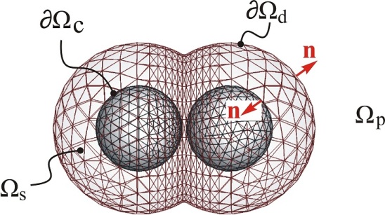
Figure 2: Illustration of the surface mesh applied to the integral computation. $\partial\Omega_{\textrm{d}}$ is the interface between the depletion zone and the bulk polymer solution. The mesh is refined near the region of overlapping depletion zones.

As a result, the corresponding integral equation can be derived for the two-layer model for the entire computation domain shown in Fig. 2, expressed as

$$\mathcal{H}v_{\emph{j}}(\mathbf{r}_{0})=\frac{1}{8\pi\eta_{\text{p}}}\int_{\partial\Omega_{\textrm{c}}}f_{\emph{i}}G_{\emph{ij}}dS$$ (26)

$$~{}~{}-\frac{1}{8\pi\lambda}\int_{\partial\Omega_{\textrm{c}}}({U_{\emph{i}}}+\varepsilon_{\emph{ijk}}{\omega_{\emph{j}}}{\ell_{\emph{k}}})T_{\emph{ijk}}n_{\emph{k}}dS+\frac{1-1/\lambda}{8\pi}\int_{\partial\Omega_{\text{d}}}v_{\emph{i}}T_{\emph{ijk}}n_{\emph{k}}dS,$$

where coefficient $\mathcal{H}=1$ for $\mathbf{r}_{0}\in\Omega_{\textrm{p}}$, $\mathcal{H}=1/\lambda$ for $\mathbf{r}_{0}\in\Omega_{\textrm{s}}$, $\mathcal{H}=({\lambda+1})/({2\lambda})$ for $\mathbf{r}_{0}\in\partial\Omega_{\textrm{d}}$, and $\mathcal{H}={1}/({2\lambda})$ for $\mathbf{r}_{0}\in\partial\Omega_{\textrm{c}}$. In the integral equation the rotational velocity $\omega_{\emph{j}}$ is unknown a priori. It can be determined by the vanishing torque applied to both isotropic spheres due to the hydrodynamic coupling,

$$\mathcal{T}_{\alpha}=\left|\int_{\partial\Omega_{\textrm{c},\alpha}}\varepsilon_{\emph{ijk}}{\ell_{\emph{j}}}{f_{\emph{k}}}dS\right|=0.$$ (27)

In summary, the integral equations (Eqs. 26 and 27) are discretized and computed for the primary variables $v_{j}(\mathbf{r}_{0}\in\partial\Omega_{\textrm{d}}),f_{j}(\mathbf{r}_{0}\in\partial\Omega_{\textrm{c}})$, and the rotational velocity for each sphere $\omega_{j}$. Once the boundary values are found, the results in the fluid domains can be obtained from Eqs. (24) and (25).

III Results and discussion

The stochastic motion of both spheres are correlated due to hydrodynamic and thermodynamic interactions. The four hydrodynamic modes represented by $F_{\|}^{\textrm{I}}$, $F_{\|}^{\textrm{II}}$, $F_{\bot}^{\textrm{I}}$, and $F_{\bot}^{\textrm{II}}$ are in general functions of the separation distance $r$, the polymer-to-sphere size ratio, and the polymer concentration. The latter quantity both affects the bulk viscosity as well as the strength of the depletion attraction. Here the two-layer model requires two input parameters, the depletion thickness $d$ and the bulk-to-solvent viscosity ratio $\lambda$. Figure 3 shows the flow patterns induced by the moving spheres corresponding to two parallel (3a and 3b) and two perpendicular (3c and 3d) modes with respect to the center-to-center line. Patterns 3a^′ to 3d^′ are corresponding typical Stokes flow for comparison. In the very dilute limit, all flow patterns are similar to the cases in a uniform fluid medium as expected (not shown here), while for a higher value of viscosity ratio, e.g. $\lambda=10$ as shown in Fig. 3b and 3d, circulations appear in the depletion zone near the particle surface due to the cage-like behavior, which is similar to what we reported earlier for the single particle tuinier2006depletion ; fan2007motion . The near-field effect has significant impact on the stress distribution and therefore the overall resistance applied to the spheres. The circulation further complicates the slip-like behavior and changes the shear and normal

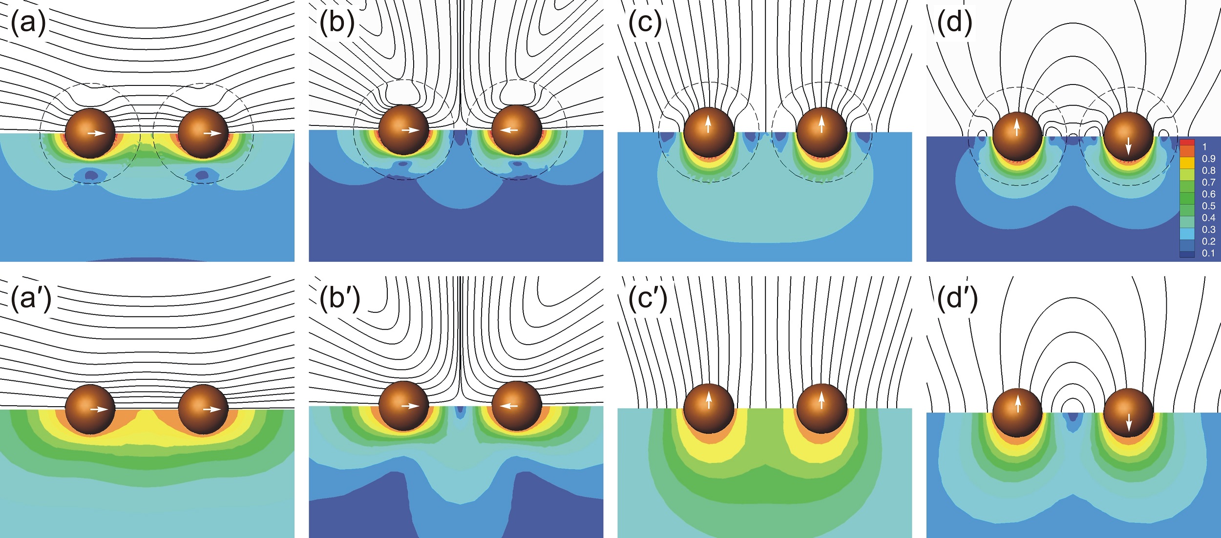
Figure 3: Streamlines and contours of the normalized velocities around interacting spheres in parallel and transverse directions, with (top panels from a to d) and without (a^′ to d^′) polymer depletion zones. Parameters used for the demonstration are: $d/a=1$, $r/a=4.5$, and $\lambda=10$.

viscous force near the front and aft surface. The overall slip-like behavior yields a fast decay of the velocity magnitude away from the particle surface. Overall, mode II has a great reduction of the resistance, whereas in mode I the reduction is less significant. As later shown in Figs. 4, the hydrodynamic correction factor approaches the resistance-distance curve dominated by the solvent viscosity (the lower bound) in modes II for both parallel and perpendicular directions.

Figures 4(a) and 4(b) show the correction factors (Eq. 17) for the hydrodynamic resistance at various scaled separation distance under parallel motion along the same (a) and opposite (b) directions. The boundary integral result is validated by the analytical approximations (the upper and lower bounds) for mode I Stimson1926 and mode II brenner1961slow written as

$$g_{\|}^{\textrm{I}}= \frac{4}{3}\sinh(\theta)\sum_{n=1}^{\infty}\frac{n(n+1)}{(2n-1)(2n+3)}$$ (29)

$$\times\left\{1-\frac{4\sinh^{2}(n+\frac{1}{2})\theta-(2n+1)^{2}\sinh^{2}\theta}{2\sinh(2n+1)\theta+(2n+1)\sinh 2\theta}\right\},$$

where $\theta=\cosh^{-1}({r}/{2a})$ and

$$g_{\|}^{\textrm{II}}= \frac{4}{3}\sinh(\theta)\sum_{n=1}^{\infty}\frac{n(n+1)}{(2n-1)(2n+3)}$$ (31)

$$\times\left\{\frac{4\cosh^{2}(n+\frac{1}{2})\theta+(2n+1)^{2}\sinh^{2}\theta}{2\sinh(2n+1)\theta-(2n+1)\sinh 2\theta}-1\right\}.$$

In the presence of the depletants, the hydrodynamic resistance is bounded by two limiting cases: solvent only and uniform polymer solution without the depletion effect (shown by the analytical data points and numerical dashed curves). The solid curve in between the upper and lower bounds illustrates the numerical results obtained for hard spheres in a non-adsorbing polymer solution described using the two-layer model. The asymptote $g\rightarrow 1.54$ is the analytical result for the resistance of a single sphere under the same depletion condition fan2007motion , and $g\rightarrow 1.0$ is the Stokes limit. For the uniform polymer solution the asymptote is $g\to\lambda$=2 (the upper bound). In the lubrication regime when two spheres are close to each other ($r/a\to 2$, mode II, 4b and 4d), the resistance approaches the solvent limit due to the dominant stress contribution from the polymer-depleted liquid film in between the spheres. However, on mode I (4a and 4c) the thin liquid film has much less influence on the resistance compared with that from the surrounding fluid. The analytical results on the perpendicular modes (square data points in Figs. 4c and 4d) are provided by O’Neill and Majumdar o1970asymmetrical , which are presented by the lower and upper bounds that we also used to validate the boundary integral results. The three data points in Fig. 4c and d The same asymptotes as presented in the parallel mode are given for large separation distance. Note that in the lubrication limit, the liquid film has less shear effect on mode II compared with the parallel motion due to the torque-free condition.

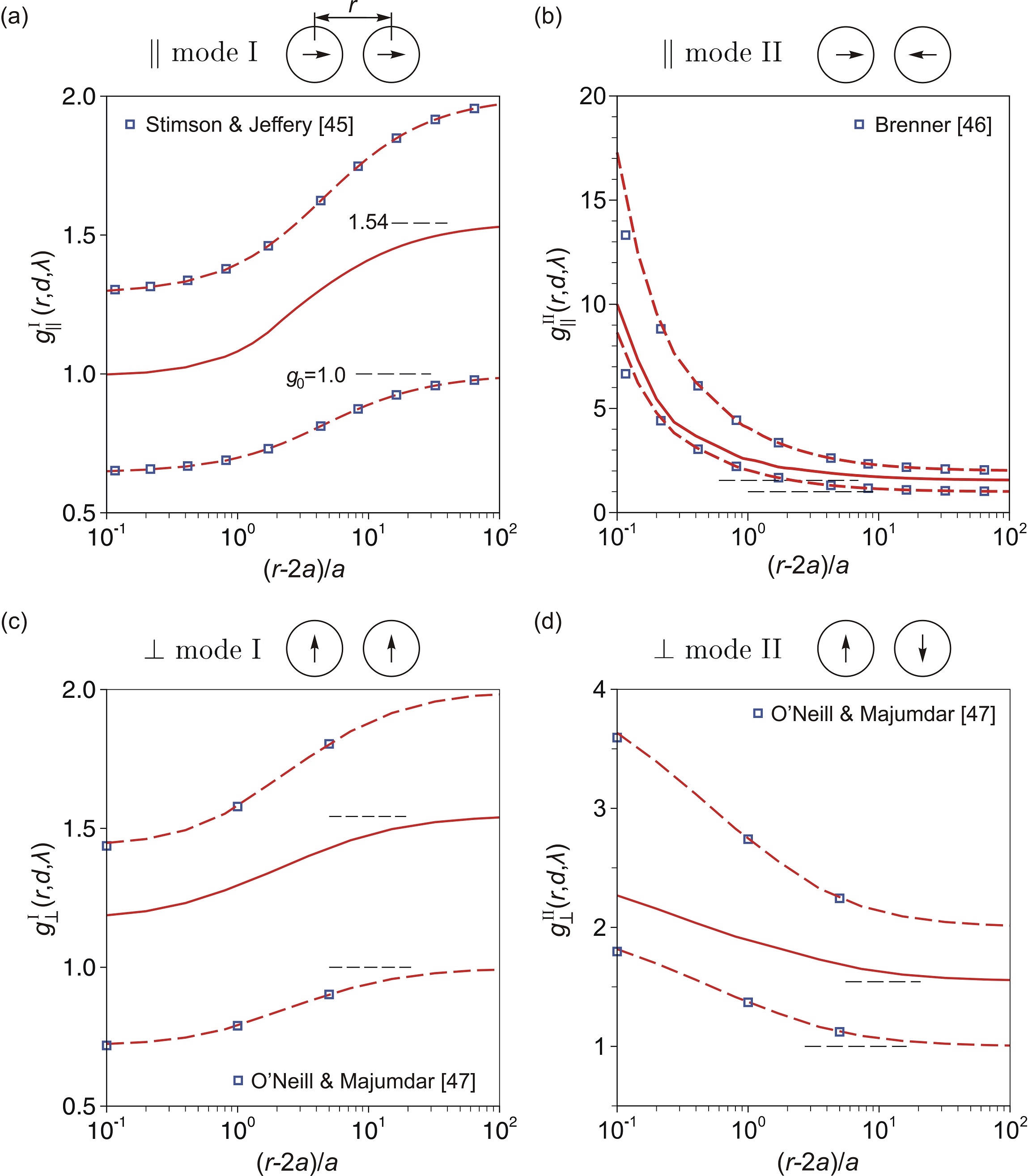
Figure 4: Semi-log plots showing the hydrodynamic correction function $g$ versus the scaled separation distance for both parallel and perpendicular motions to the center-to-center line along the same (a, c) and opposite (b, d) directions. The square data points are the exact series solution for a uniform solvent (lower bound) and uniform bulk solution (upper bound) Stimson1926 ; brenner1961slow ; o1970asymmetrical . The dashed-lines indicate boundary integral results as a numerical validation. The solid curves show the results for hard spheres in a nonadsorbing polymer solution with depletion layer described using the two-layer model.

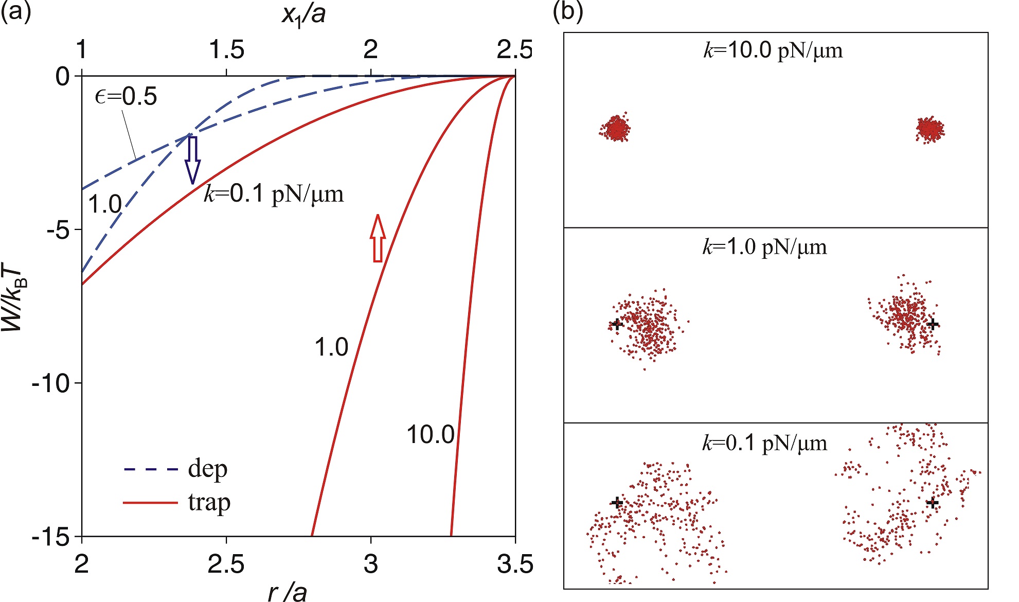
Figure 5: (a) The comparison of the potential of the optical trap applied to the particle with the trapping center located at $x_{1}/a=2.5$ and the polymer depletion potential between two spheres versus the center-to-center separation distance $r/a$ (=2 when spheres are in contact with each other). (b) A test run of Brownian simulations with data points showing the particle position per 200 time steps. The total simulation time is 2 s. In this test case, $d/a=1$ and $\lambda=2$. The centers of two traps are indicated by the plus signs.

In Fig. 5 we compare typical depletion and trapping harmonic potentials applied to the hard spheres. In general the attractive force is enhanced by a higher polymer concentration if the overlap volume remains the same. However, the depletion thickness reduces as the bulk polymer concentration increases, which reduces the overlap volume and suppresses the attractive force. The value for the stiffness of the optical trap has a significant caging effect on the Brownian motion of both spheres as the simulation results illustrated in Fig. 5(b). Parameters used in the simulation are: time step $\triangle t=$28.5 $\mu$s, radius $a=500$ nm, polymer concentration $\epsilon=$ 0.5, and depletion thickness $d/a=0.69$ that corresponds to $R_{g}/a=1$. The distance between the traps and the initial particle separation distance are set to $r/a$=2.5. Both hydrodynamic and depletion effects are taken into account, the data points clearly shows the attractive depletion effect on the probability distribution of the spheres, with the characteristic distribution length inversely proportional to the square root of $k$. Next we consider the correlation analysis that better characterizes the ensemble results.

As a baseline comparison for the correlation analysis, the long-time autocorrelation of the random displacement is considered for a single Brownian sphere with and without polymer depletion, which can be formulated by the analytical result doi1988theory :

$$\langle x(t)x(0)\rangle=\frac{k_{\textrm{B}}T}{k}\left[\exp\left(-\frac{t}{\tau}\right)\right],$$ (32)

where ${k_{\textrm{B}}T}/{k}$ measures the thermal energy versus the strength of the harmonic potential, and more importantly the decorrelation time depends on corrected hydrodynamic resistance, and the harmonic potential,

$$\tau=\frac{6\pi\eta_{\textrm{s}}ag_{0}(\lambda,d)}{k},$$ (33)

and the mean square displacement can also be formulated as

$$\langle x(t)^{2}\rangle=\frac{k_{\textrm{B}}T}{k}\left[1-\exp\left(-\frac{2t}{\tau}\right)\right].$$ (34)

For spheres with a radius of 500 nm and an optical trap with stiffness $k=$10, 1, and 0.1 pN/$\mu$m, the corresponding characteristic length squares for the autocorrelation function $\sqrt{k_{\textrm{B}}T/k}$ are approximately 20, 65, and 200 nm in a pure solvent. The corresponding decorrelation times are 1, 10, and 100 ms, respectively, whereas in a dilute polymer solution, the decorrelation times increases slightly to 1.33, 13.3, and 133 ms in a pure solvent.

This increase is due to the enhanced viscous resistance or slower motion of the particles. Although the discussion here is applicable to an isolated particle, the resulting characteristic distribution length is about the same order of magnitude as the diffusive length (independent of hydrodynamic interactions) observed in Fig. 5b because the total simulation time (2 s) is far beyond the decorrelation time. In other words, the depletion effect shifts the probability distribution of the random walk instead of altering the characteristic diffusive length. If the bulk viscosity is used instead of the two-layer depletion model, the decorrelation times would be 1.53, 15.3, and 153 ms, respectively. One can speculate that the result is applicable for colloid-polymer dispersions with colloid volume fraction $\ll 10^{-5}$ or an averaged pair separation distance $\gg 100a$.

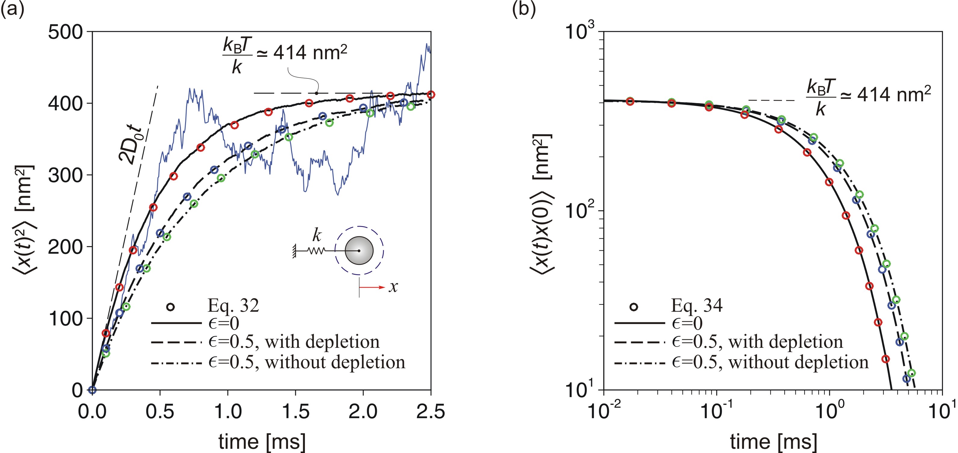
Figure 6: Brownian simulation results for a single sphere showing the mean square displacement versus time (a) and the long-time autocorrelation function (b) of the random motion of the isolated sphere in pure solvent ($\epsilon=0$) and dilute polymer solution ($\epsilon=0.5$) with and without the polymer depletion effect under ambient temperature. The thin blue curve is the average from 100 samples, and the thick black curve is the result from averaging over 10⁴ samples .

In Fig. 6 results are shown for the random motion of a tapped single sphere. In Fig. 6a the mean square displacement is plotted versus time in a pure solvent and in polymer solutions with and without depletion. In Fig. 6a, the thin blue curve is the ensemble average over 100 samples which is considerably noisy compared to the thick black curve from the average over 10⁴ samples. Parameters applied to the simulations are: $a$=500 nm, $k$=10 pN/$\mu$m, $R_{g}/a$=1, viscosity ratio $\lambda$=1.611, depletion thickness $d/a$=0.638 for the normalized polymer concentration $\epsilon=0.5$, and the time step for the Brownian simulation $\Delta t=$3$\times 10^{-5}$ s. In Fig. 6b, the data points represent the analytical solution and the lines are from Brownian simulations. The sample size for computing the autocorrelation function is sufficiently large by considering total simulation time around 10 s. The decay time can be obtained from the best fit to the numerical results based on the exponential decay given by Eq. 33. The computed versus analytical decay times are 0.9424, 1.3298, and 1.5183 ms for $\epsilon=0$, $\epsilon=0.5$ with depletion, and $\epsilon=0.5$ without depletion, respectively. Under the same stiffness, the large viscous effect essentially increases the decorrelation time. At shorter times the difference is negligible, whereas at longer times the viscous effect enhances the autocorrelation along the harmonic force direction as expected. Therefore, the case without the depletion effect has the largest decorrelation time (and thus the $g$ factor) due to the highest viscous resistance.

For the pair interaction, the analytical pair correlation function of spheres in homogeneous fluids is available bartlett2001measurement ; meiners1999direct . A straightforward extension of this result to incorporate the depletion effect for the two-dimensional movement of a pair of spheres in $x-$ and $z-$direction ($y$ and $z$ are equivalent) can be written as

$$\begin{bmatrix}\dot{x}_{1}\\ \dot{z}_{1}\\ \dot{x}_{2}\\ \dot{z}_{2}\end{bmatrix}=\begin{bmatrix}1+A^{\textrm{s}}&0&A^{\textrm{c}}&0\\ 0&1+B^{\textrm{s}}&0&B^{\textrm{c}}\\ A^{\textrm{c}}&0&1+A^{\textrm{s}}&0\\ 0&B^{\textrm{c}}&0&1+B^{\textrm{s}}\end{bmatrix}\begin{bmatrix}-kx_{1}-F^{\textrm{dep}}+F^{\textrm{B}}_{1}\\ -kz_{1}+F^{\textrm{B}}_{1}\\ -kx_{2}+F^{\textrm{dep}}+F^{\textrm{B}}_{2}\\ -kz_{2}+F^{\textrm{B}}_{2}\end{bmatrix}/{(6\pi\eta_{\textrm{s}}ag_{0})}.$$ (35)

The eigenvalues of the mobility tensor are $1/6\pi\eta_{\textrm{s}}ag^{\textrm{I}}_{\|}$, $1/6\pi\eta_{\textrm{s}}ag_{\|}^{\textrm{II}}$, $1/6\pi\eta_{\textrm{s}}ag_{\bot}^{\textrm{I}}$, and $1/6\pi\eta_{\textrm{s}}ag_{\bot}^{\textrm{II}}$, which represent the inverse hydrodynamic resistance in the four hydrodynamic modes with boundary conditions described in Eq. 22. The four principal vectors are $Y_{\|}^{\textrm{I}}=x_{1}+x_{2}$, $Y_{\|}^{\textrm{II}}=x_{1}-x_{2}$, $Y_{\bot}^{\textrm{I}}=z_{1}+z_{2}$, and $Y_{\bot}^{\textrm{II}}=z_{1}-z_{2}$, representing the common (collective, mode I) and relative (mode II) motions of spheres in both parallel and perpendicular directions, respectively. The eigenvector lead to the following autocorrelation functions for the pair interactions under the four eigenmodes:

$$\displaystyle{\langle Y_{\|}^{\textrm{I}}(t)Y_{\|}^{\textrm{I}}(0)\rangle=\frac{2k_{B}T}{k}\left[\exp\left(-\frac{t}{\tau_{\|}^{\textrm{I}}}\right)\right]},$$ (36)

$$\displaystyle{\langle Y_{\|}^{\textrm{II}}(t)Y_{\|}^{\textrm{II}}(0)\rangle=\left(\frac{2{F^{\textrm{dep}}}}{k}\right)^{2}+\frac{2k_{B}T}{k}\left[\exp\left(-\frac{t}{\tau_{\|}^{\textrm{II}}}\right)\right],}$$

$$\displaystyle{\langle Y_{\bot}^{\textrm{I}}(t)Y_{\bot}^{\textrm{I}}(0)\rangle=\frac{2k_{B}T}{k}\left[\exp\left(-\frac{t}{\tau_{\bot}^{\textrm{I}}}\right)\right],\quad\textrm{and}}$$

$$\displaystyle{\langle Y_{\bot}^{\textrm{II}}(t)Y_{\bot}^{\textrm{II}}(0)\rangle=\frac{2k_{B}T}{k}\left[\exp\left(-\frac{t}{\tau_{\bot}^{\textrm{II}}}\right)\right],}$$

where the individual decay time for each mode are $\tau_{\|}^{\textrm{I}}=6\pi\eta_{\textrm{s}}g^{\textrm{I}}_{\|}/k$, $\tau_{\|}^{\textrm{II}}=6\pi\eta_{\textrm{s}}g^{\textrm{II}}_{\|}/k$, $\tau_{\bot}^{\textrm{I}}=6\pi\eta_{\textrm{s}}g^{\textrm{I}}_{\bot}/k$, and $\tau_{\bot}^{\textrm{II}}=6\pi\eta_{\textrm{s}}g^{\textrm{II}}_{\bot}/k$. The four decay times of the corresponding principal modes all reduce to the single particle limit as the separation distance becomes large, e.g., $r/a>\mathcal{O}(10^{2})$. Figure 7 demonstrates autocorrelation functions under the four principal modes with various concentration and separation distance. Comparing Figs 7a with 7b, and 7c with 7d, in both directions the decorrelation times in mode I (the collective motion, 7a and 7c) are always shorter than mode II (relative motion, 7b and 7d). The reason is because the hydrodynamic resistance is always higher in the relative motion, which slows down the particle motion more significantly especially in the lubrication regime.

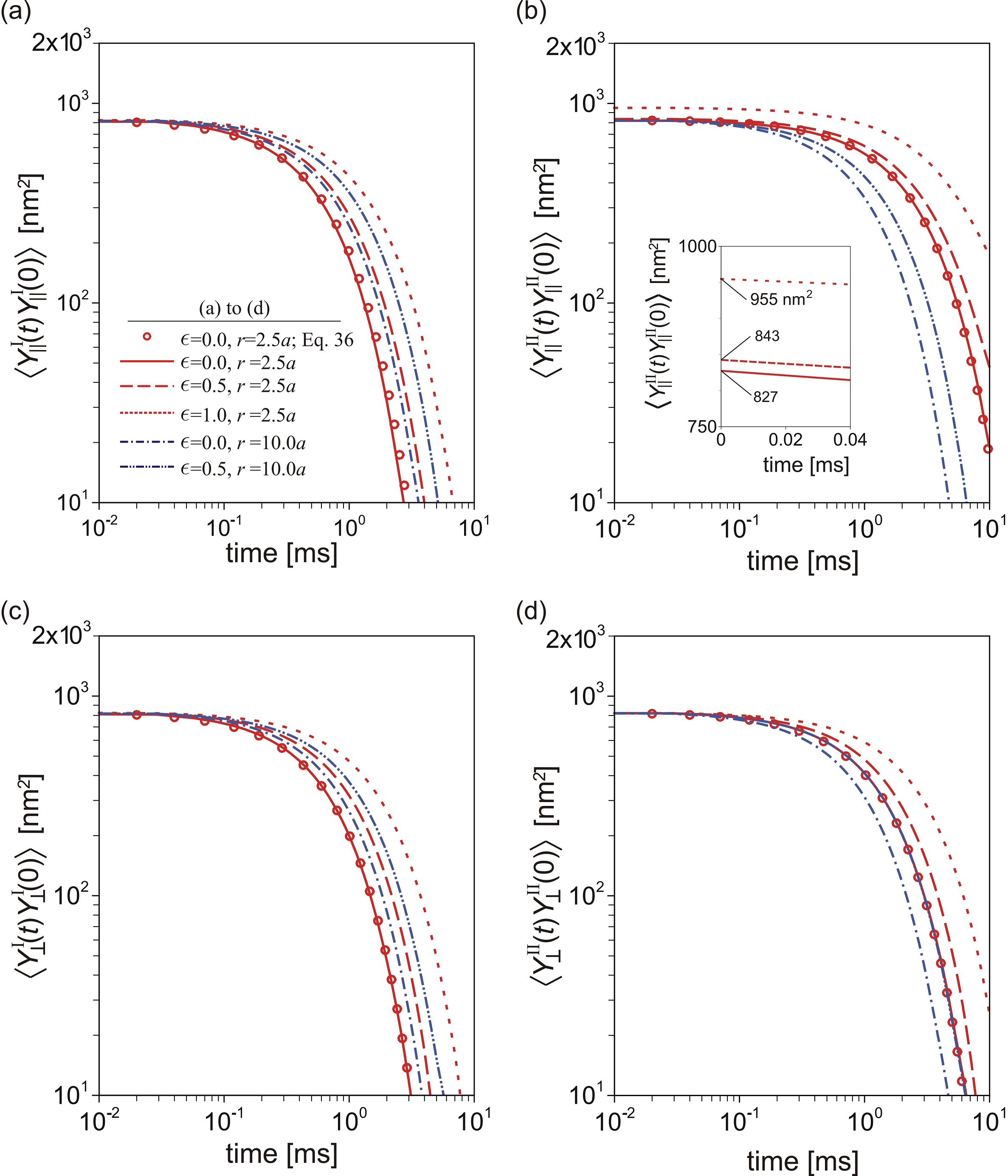
Figure 7: Autocorrelation functions of the displacement along the four principal directions. The data points represent the analytical results (Eq. 29) using the mobility functions given by Batchelor batchelor1976brownian . Parameters for particles and polymer are the same as in Fig. 6.

When comparing parallel to perpendicular motions, in mode I the behavior is similar for both motions because the depletion effect has been canceled in both eigenmodes $Y_{\|}^{\textrm{I}}$ and $Y_{\|}^{\textrm{II}}$ and therefore only the hydrodynamic effect plays a role in mode I, in which the correction factors in parallel and perpendicular motions have similar values. In the eigenmode II parallel motion (7b), the autocorrelation function includes the decomposed contributions from two sources, the depletion force and the hydrodynamic resistance. The polymer depletion effect changes the equilibrium position of spheres along $Y_{\|}^{\textrm{II}}$ direction with a magnitude of $2{F^{\textrm{dep}}}/k$. This shifts the autocorrelation of spheres’ movement in parallel mode II with a magnitude of $4({F^{\textrm{dep}}}/k)^{2}$. In nearby location of optical traps ($r/a\simeq 2.5$) the decorrelation time of motion of spheres is enhanced. In mode II, the increase of the decorrelation time is more pronounced in parallel (7b) than in the perpendicular (7d) directions. It is due to the larger hydrodynamic correction factor $g_{\|}^{\textrm{II}}$ compared to $g_{\bot}^{\textrm{II}}$, which can be speculated from the $g$-factor plots (Figs. 4b, 4c). With increasing polymer concentration $\epsilon$ the decorrelation time in all modes will increase due to larger viscous resistance force. In principle one may compute the $g$ factor and the decay time of displacement autocorrelation functions in four principal directions by experimentally measuring the auto- and cross-correlation of displacements. It is also valuable to validate the attractive potential between two hard spheres from the dynamic view point through the shift $4({F^{\textrm{dep}}}/k)^{2}$ in the autocorrelation function ($Y_{\|}^{\textrm{II}}$).

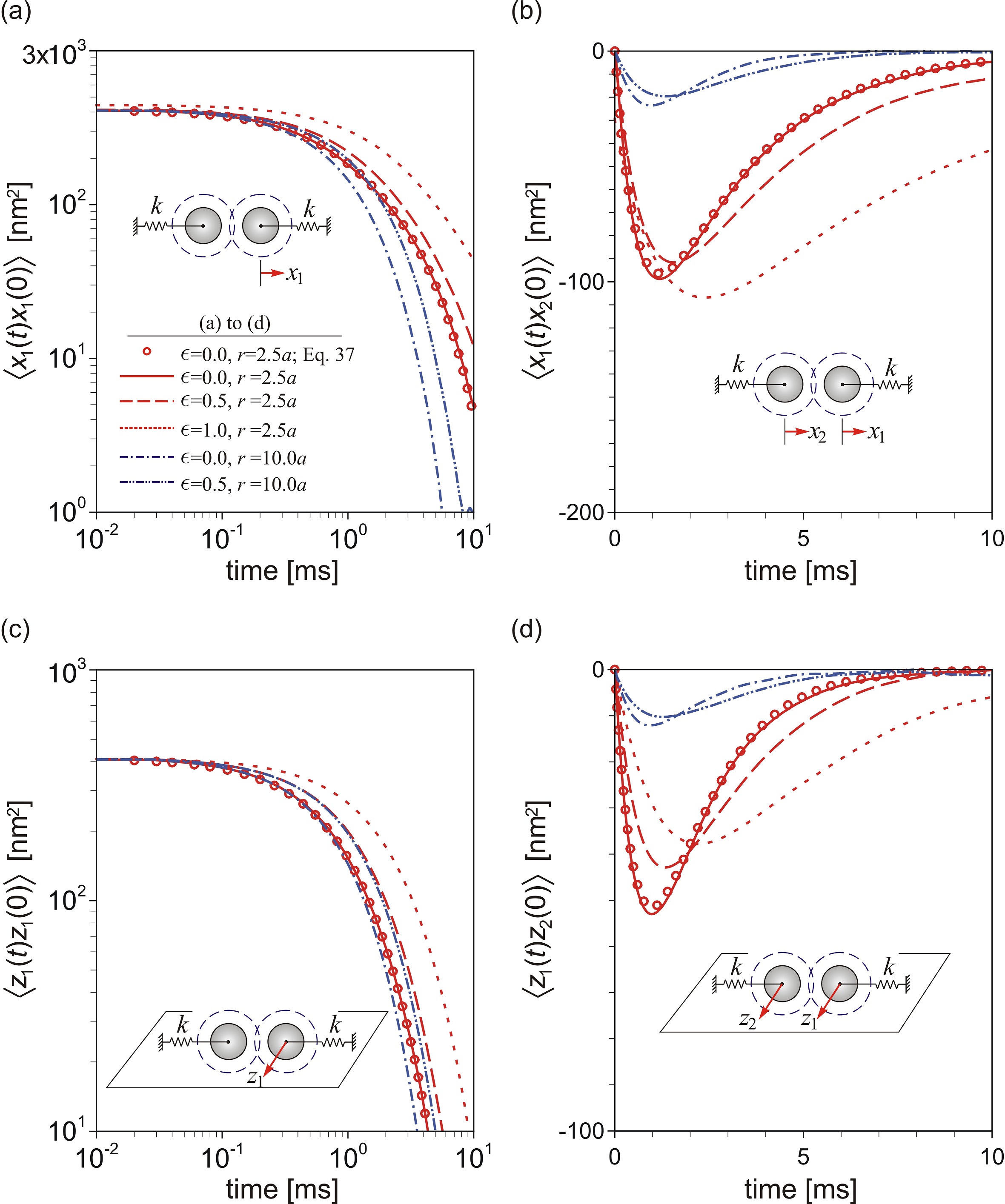
Figure 8: Correlation functions of the displacement of two trapped spheres in the $xz-$plane under the influence of depletion layers. Parameters used for particles and polymer conditions are the same as in Fig. 6.

In physical space, the correlation functions on the $x,z$ plane are

$$\displaystyle{\langle x_{1}(t)x_{1}(0)\rangle=\left(\frac{{F^{\textrm{dep}}}}{k}\right)^{2}+\frac{k_{B}T}{2k}\left[\exp\left(-\frac{t}{\tau_{\|}^{\textrm{I}}}\right)+\exp\left(-\frac{t}{\tau_{\|}^{\textrm{II}}}\right)\right],}$$ (37)

$$\displaystyle{\langle x_{1}(t)x_{2}(0)\rangle=-\left(\frac{{F^{\textrm{dep}}}}{k}\right)^{2}+\frac{k_{B}T}{2k}\left[\exp\left(-\frac{t}{\tau_{\|}^{\textrm{I}}}\right)-\exp\left(-\frac{t}{\tau_{\|}^{\textrm{II}}}\right)\right],}$$

$$\displaystyle{\langle z_{1}(t)z_{1}(0)\rangle=\frac{k_{B}T}{2k}\left[\exp\left(-\frac{t}{\tau_{\bot}^{\textrm{I}}}\right)+\exp\left(-\frac{t}{\tau_{\bot}^{\textrm{II}}}\right)\right],}\quad\textrm{and}$$

$$\displaystyle{\langle z_{1}(t)z_{2}(0)\rangle=\frac{k_{B}T}{2k}\left[\exp\left(-\frac{t}{\tau_{\bot}^{\textrm{I}}}\right)-\exp\left(-\frac{t}{\tau_{\bot}^{\textrm{II}}}\right)\right].}$$

The correlation results are plotted in Fig 8. Note correlation functions above include the self- and cross-correlations in the principle directions, and can be computed by

$$\displaystyle{\langle x_{1}(t)x_{1}(0)\rangle=\frac{1}{4}\left[\langle Y_{\|}^{\textrm{I}}(t)Y_{\|}^{\textrm{I}}(0)\rangle+\langle Y_{\|}^{\textrm{I}}(t)Y_{\|}^{\textrm{II}}(0)\rangle+\langle Y_{\|}^{\textrm{I}}(0)Y_{\|}^{\textrm{II}}(t)\rangle+\langle Y_{\|}^{\textrm{II}}(t)Y_{\|}^{\textrm{II}}(0)\rangle\right]},$$ (38)

and

$$\displaystyle{\langle x_{1}(t)x_{2}(0)\rangle=\frac{1}{4}\left[\langle Y_{\|}^{\textrm{I}}(t)Y_{\|}^{\textrm{I}}(0)\rangle-\langle Y_{\|}^{\textrm{I}}(t)Y_{\|}^{\textrm{II}}(0)\rangle+\langle Y_{\|}^{\textrm{I}}(0)Y_{\|}^{\textrm{II}}(t)\rangle-\langle Y_{\|}^{\textrm{II}}(t)Y_{\|}^{\textrm{II}}(0)\rangle\right]}.$$ (39)

The same formulations are applied to find the correlations functions in the $z$-direction. Along the parallel direction (Fig. 8a and 8b) the auto- and cross-correlation functions at $t=0$ deviates from $k_{\textrm{B}}T/k$ (auto) and zero (cross) with an amount of $({F^{\textrm{dep}}}/k)^{2}$, however, the two decorrelation time scales involved maybe difficult to distinguish from each other. Similarly in the perpendicular direction, the correlation functions are determined by two time scales that originate from the two hydrodynamic modes. Considering the decayed hydrodynamic interactions, at very long lag time all correlations vanish, while at zero lag time the cross-correlation vanishes, implying that apparently the particle does not feel the presence of another particle at the beginning due to the mutual cancellation of collective and relative motions. The entropic force has a finite influence on both correlations. They are always anti-correlated because the first mode (collective motion) always decays faster than the second mode (relative motion) due to its less resistance. In other words, this relative motion dominates the relevance of the displacements of both particles after certain lag time, and the pair interaction behaves like in its second or anticorrelated mode. This fact is not to be confused with the intuition obtained from a steady mobility analysis.

The largest anticorrelation appears at

$$t_{\textrm{min},\|}=\frac{\tau^{\textrm{I}}_{\|}\tau^{\textrm{II}}_{\|}}{\tau^{\textrm{I}}_{\|}-\tau^{\textrm{II}}_{\|}}\ln\left(\frac{\tau^{\textrm{I}}_{\|}}{\tau^{\textrm{II}}_{\|}}\right)=\frac{g^{\textrm{I}}_{\|}g^{\textrm{II}}_{\|}}{g^{\textrm{I}}_{\|}-g^{\textrm{II}}_{\|}}\ln\left(\frac{g^{\textrm{I}}_{\|}}{g^{\textrm{II}}_{\|}}\right).$$ (40)

The same formulation is applicable for the perpendicular direction. The depth of the anticorrelation in parallel direction versus the distance of optical traps is predicted in Fig. 9. At large separation distance the motion obviously is uncorrelated. At short separation distance, the increase of the depth is due to both hydrodynamic and depletion interactions. Without the depletion effect, the analytical results from Batchelor’s approximation (solid curves) is somewhat higher than the numerical simulation (black circles) because the approximation yields a relative lower lubrication force, which enhances the influence of the relative motion. Consistent results are shown by the two blue lines in Fig. 8b and 8d, in which the higher viscosity gives a shallower anticorrelation. By bringing the pair particles closer to each other, the minimum value for $\langle x_{1}(t)x_{2}(0)\rangle$ is lower at small $a/r$ and then higher for the polymer solution cases with depletion effect (red squares and blue diamonds) compared with the solvent-only case (black circles). The overlapping of the depletion zones appears at $a/r$$\approx$0.31 ($\epsilon=0.5$) and $a/r$$\approx$0.38 ($\epsilon=1.0$). Without depletion zones, the uniform polymer solution case, the hydrodynamic resistance experience by the spheres is higher because the higher bulk viscosity simply gives a shallower anticorrelation. Into the overlap region, the entropic force brings particles toward each other and enhances anticorrelation mode. This effect is further enhanced by bringing the spheres closer. The complicated flow pattern and resistance in the two-layer model has relatively much less contribution compared with the entropic effect on the anticorrelation depth. Experimental validation is needed to validate this result.

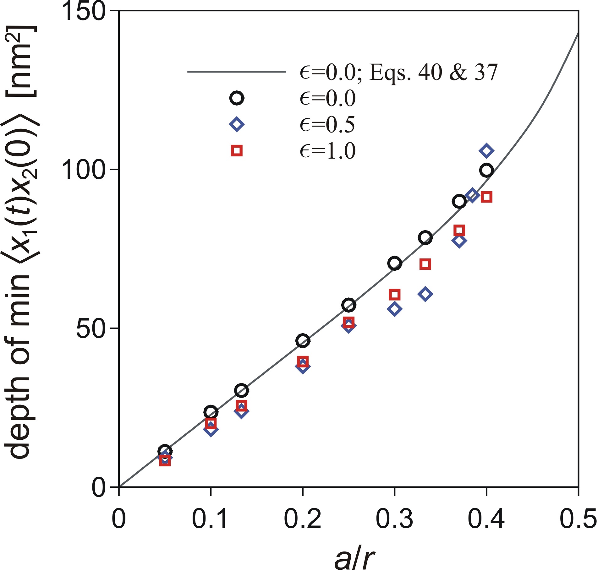
Figure 9: The maximum value of the anticorrelation in the parallel direction versus the center-to-center separation distance. The limit $a/r=0$ indicates an isolated particle, while $a/r=0.5$ means both particles are in contact with each other. The reference curve is the analytical approximation based on the mobility function for the solvent-only case.

IV Conclusion

We presented a theoretical description that enables to characterize the stochastic motions of a pair of hard spheres in non-adsorbing polymer solutions. Based on a two-layer approximation for the polymer depletion effect, the hydrodynamic mobility tensor is resolved by the boundary integral analysis, which determines the corresponding time evolution of stochastic displacements that are consistent with the fluctuation-dissipation theorem. We first find that the presence of depletion zones significantly modifies the hydrodynamic interactions between two moving spheres. Polymer depletion is found to shift the probability distribution of the random walks of two trapped spheres. The resulting auto- and cross-correlation functions are presented in the principal modes, which clearly identify the decomposed entropic and hydrodynamic effects on the dynamic behavior of two hard spheres under the influence of added polymers to the solvent for various particle separation distances. In the presence of depletants, the cross-correlation of the particle displacements is weakened in a way that higher viscosity slows down the motion significantly and lengthens the hydrodynamic decay time. However, the appearance of the depletion zone reduces this viscous effect. Finally, the cross-correlation is significantly enhanced when the depletion zones overlap.

Acknowledgments  M. Karzar-Jeddi and T.-H. Fan acknowledge the support from NSF CMMI-0952646, R. Tuinier thanks DSM for support, and T. Taniguchi acknowledges the support from JSF.

APPENDIX A

The divergence of the diffusivity tensor (Eqs. 12 and 13) can be expressed as

$$\frac{\partial}{\partial\mathbf{r}_{\alpha}}\cdot\mathbf{D}_{\alpha\alpha}= \frac{D_{0}}{g_{0}}\left.\Bigg{[}\frac{\mathbf{r}_{\alpha\beta}\mathbf{r}_{\alpha\beta}}{r^{2}}\cdot\frac{\partial A^{\textrm{s}}}{\partial\mathbf{r}_{\alpha}}+\left(\mathbf{I}-\frac{\mathbf{r}_{\alpha\beta}\mathbf{r}_{\alpha\beta}}{r^{2}}\right)\cdot\frac{\partial B^{\textrm{s}}}{\partial\mathbf{r}_{\alpha}}\right.$$

$$~{}~{}+\left.(A^{\textrm{s}}-B^{\textrm{s}})\mathbf{r}_{\alpha\beta}\mathbf{r}_{\alpha\beta}\cdot\frac{\partial~{}~{}}{\partial\mathbf{r}_{\alpha}}\left(\frac{1}{r^{2}}\right)+\left(\frac{A^{\textrm{s}}-B^{\textrm{s}}}{r^{2}}\right)\frac{\partial~{}~{}}{\partial\mathbf{r}_{\alpha}}\cdot(\mathbf{r}_{\alpha\beta}\mathbf{r}_{\alpha\beta})\right.\Bigg{]},$$

where $\alpha,\beta=1,2$ and $\alpha\neq\beta$, $\mathbf{r}_{\alpha\beta}=\mathbf{r}_{\beta}-\mathbf{r}_{\alpha}$, and $r=|\mathbf{r}_{\beta}-\mathbf{r}_{\alpha}|$. By simplifying the differential terms on the right

$$\frac{\partial}{\partial\mathbf{r}_{\alpha}}\cdot\mathbf{D}_{\alpha\alpha} = \frac{D_{0}}{g_{0}}\left.\Bigg{\{}\frac{\mathbf{r}_{\alpha\beta}\mathbf{r}_{\alpha\beta}}{r^{2}}\cdot\left(\frac{-\mathbf{r}_{\alpha\beta}}{r}\frac{\partial A^{\textrm{s}}}{\partial r}\right)+\left(\mathbf{I}-\frac{\mathbf{r}_{\alpha\beta}\mathbf{r}_{\alpha\beta}}{r^{2}}\right)\cdot\left(\frac{-\mathbf{r}_{\alpha\beta}}{r}\frac{\partial B^{\textrm{s}}}{\partial r}\right)\right.$$

$$~{}~{}~{}~{}+\left.(A^{\textrm{s}}-B^{\textrm{s}})\mathbf{r}_{\alpha\beta}\mathbf{r}_{\alpha\beta}\cdot\left(\frac{2\mathbf{r}_{\alpha\beta}}{r^{4}}\right)+\frac{A^{\textrm{s}}-B^{\textrm{s}}}{r^{2}}\Bigg{[}-\mathbf{r}_{\alpha\beta}\cdot\mathbf{I}+\mathbf{r}_{\alpha\beta}\left(\frac{\partial~{}~{}}{\partial\mathbf{r}_{\alpha}}\cdot\mathbf{r}_{\alpha\beta}\right)\Bigg{]}\right.\Bigg{\}}$$

$$= \frac{D_{0}}{g_{0}}\Bigg{[}\frac{-r^{2}\mathbf{r}_{\alpha\beta}}{r^{3}}\frac{\partial A^{\textrm{s}}}{\partial r}+\frac{-\mathbf{r}_{\alpha\beta}}{r}\frac{\partial B^{\textrm{s}}}{\partial r}+\frac{r^{2}\mathbf{r}_{\alpha\beta}}{r^{3}}\frac{\partial B^{\textrm{s}}}{\partial r}+\frac{2(A^{\textrm{s}}-B^{\textrm{s}})}{r^{2}}\mathbf{r}_{\alpha\beta}+\frac{-4(A^{\textrm{s}}-B^{\textrm{s}})}{r^{2}}\mathbf{r}_{\alpha\beta}\Bigg{]}.$$

Therefore

$$\frac{\partial}{\partial\mathbf{r}_{\alpha}}\cdot\mathbf{D}_{\alpha\alpha} = \frac{-D_{0}}{g_{0}}\left[\frac{\partial A^{\textrm{s}}}{\partial r}+\frac{2(A^{\textrm{s}}-B^{\textrm{s}})}{r}\right]\frac{\mathbf{r}_{\alpha\beta}}{r}.$$ (A3)

Similarly, the divergence of the mutual diffusivity tensor can be expressed as

$$\frac{\partial}{\partial\mathbf{r}_{\beta}}\cdot\mathbf{D}_{\alpha\beta} = \frac{D_{0}}{g_{0}}\Bigg{\{}\frac{\mathbf{r}_{\alpha\beta}\mathbf{r}_{\alpha\beta}}{r^{2}}\cdot\left(\frac{\mathbf{r}_{\alpha\beta}}{r}\frac{\partial A^{\textrm{c}}}{\partial r}\right)+\left(\mathbf{I}-\frac{\mathbf{r}_{\alpha\beta}\mathbf{r}_{\alpha\beta}}{r^{2}}\right)\cdot\left(\frac{\mathbf{r}_{\alpha\beta}}{r}\frac{\partial B^{\textrm{c}}}{\partial r}\right)$$

$$~{}~{}~{}~{}+(A^{\textrm{c}}-B^{\textrm{c}})\mathbf{r}_{\alpha\beta}\mathbf{r}_{\alpha\beta}\cdot\left(\frac{-2\mathbf{r}_{\alpha\beta}}{r^{4}}\right)+\frac{A^{\textrm{c}}-B^{\textrm{c}}}{r^{2}}\Bigg{[}\mathbf{r}_{\alpha\beta}\cdot\mathbf{I}+\mathbf{r}_{\alpha\beta}\left(\frac{\partial~{}~{}}{\partial\mathbf{r}_{\beta}}\cdot\mathbf{r}_{\alpha\beta}\right)\Bigg{]}\Bigg{\}}.$$

Which simplifies to Eq. 19,

$$\frac{\partial}{\partial\mathbf{r}_{\beta}}\cdot\mathbf{D}_{\alpha\beta} = \frac{D_{0}}{g_{0}}\left[\frac{\partial A^{\textrm{c}}}{\partial r}+\frac{2(A^{\textrm{c}}-B^{\textrm{c}})}{r}\right]\frac{\mathbf{r}_{\alpha\beta}}{r}.$$ (A5)

In a uniform fluid ($\lambda$=1), $A^{\textrm{s}}$=$B^{\textrm{s}}$=0, $A^{\textrm{c}}=3a/2r$, $B^{\textrm{c}}=3a/4r$ for the Oseen tensor, and $A^{\textrm{s}}$=$B^{\textrm{s}}$=0, $A^{\textrm{c}}=3a/2r-a^{3}/r^{3}$, $B^{\textrm{c}}=3a/4r+a^{3}/2r^{3}$ for Rotne-Prager tensor. For both cases $\partial\mathbf{D}_{\alpha\alpha}/\partial\mathbf{r}_{\alpha}=\partial\mathbf{D}_{\alpha\beta}/\partial\mathbf{r}_{\beta}=0$ are applicable in Brownian motion simulations..

References

- [1] S.B. Zimmerman, and A.P. Minton, Macromolecular crowding: biochemical, biophysical, and physiological consequences, Annu. Rev. Biophys. Biomol. Struct., 22(1):27–65, 1993.
- [2] R.J. Ellis, and A.P. Minton, Join the crowd, Nature, 425:27–28, 2003.
- [3] J.-L. Doublier, C. Garnier, D. Renard, and C. Sanchez, Protein–polysaccharide interactions, Curr. Opin. Colloid Interface Sci., 5(3):202–214, 2000.
- [4] S. Tanaka, and M. Ataka, Protein crystallization induced by polyethylene glycol: A model study using apoferritin, J. Chem. Phys., 117(7):3504–3510, 2002.
- [5] L. Rossi, S. Sacanna, W.T.M. Irvine, P.M. Chaikin, D.J. Pine, and A.P. Philipse, Cubic crystals from cubic colloids, Soft Matter, 7(9):4139–4142, 2011.
- [6] S. Asakura, and F. Oosawa, On interaction between two bodies immersed in a solution of macromolecules, J. Chem. Phys., 22:1255–1256, 1954.
- [7] S. Asakura, and F. Oosawa, Interaction between particles suspended in solutions of macromolecules, J. of Polym. Sci., 33(126):183–192, 1958.
- [8] A. Vrij, Polymers at interfaces and the interactions in colloidal dispersions, Pure & Appl. Chem., 48(4):471–483, 1976.
- [9] A.P. Gast, C.K. Hall, and W.B. Russel, Polymer-induced phase separations in nonaqueous colloidal suspensions, J. Colloid Interface Sci., 96(1):251–267, 1983.
- [10] H.N.W. Lekkerkerker, W.C.-K. Poon, P.N. Pusey, A. Stroobants, and P.B. Warren, Phase behaviour of colloid+polymer mixtures, Europhys. Lett., 20(6):559–564, 1992.
- [11] H.N.W. Lekkerkerker, and A. Stroobants, Phase behaviour of rod-like colloid+ flexible polymer mixtures, Il Nuovo Cimento D, 16(8):949–962, 1994.
- [12] T. Koda, and S. Ikeda, Test of the scaled particle theory for aligned hard spherocylinders using monte carlo simulation, J. Chem. Phys., 116(13):5825–5830, 2002.
- [13] W.C.K. Poon, The physics of a model colloid–polymer mixture, J. Phys.: Condens. Matter, 14(33):R859–R880, 2002.
- [14] G.J. Fleer, and R. Tuinier, Analytical phase diagrams for colloids and non-adsorbing polymer. Adv. Colloid Interface Sci., 143(1):1–47, 2008.
- [15] R. Tuinier, J.K.G. Dhont, and T.-H. Fan, How depletion affects sphere motion through solutions containing macromolecules, Europhys. Lett., 75(6):929-935, 2006.
- [16] R. Verma, J.C. Crocker, T.C. Lubensky, and A.G. Yodh, Entropic colloidal interactions in concentrated DNA solutions, Phys. Rev. Lett., 81(18):4004–4007, 1998.
- [17] R. Verma, J.C. Crocker, T.C. Lubensky, and A.G. Yodh, Attractions between hard colloidal spheres in semiflexible polymer solutions, Macromolecules, 33(1):177–186, 2000.
- [18] M. Fuchs, and K.S. Schweizer, Structure of colloid-polymer suspensions, J. Phys.: Condens. Matter, 14(12):R239–R269, 2002.
- [19] J. Dzubiella, C.N. Likos, and H. Löwen, Phase behavior and structure of star-polymer–colloid mixtures, J. Chem. Phys., 116(21):9518–9530, 2002.
- [20] K.J. Mutch, J.S. van Duijneveldt, and J. Eastoe, Colloid–polymer mixtures in the protein limit, Soft Matter, 3(2):155–167, 2007.
- [21] D. Kleshchanok, R. Tuinier, and P.R. Lang, Direct measurements of polymer-induced forces, J. Phys.: Condens. Matter, 20(7):073101, 2008.
- [22] E. Donath, A. Krabi, M. Nirschl, V.M. Shilov, M.I. Zharkikh, and B. Vincent, Stokes friction coefficient of spherical particles in the presence of polymer depletion layers. Analytical and numerical calculations, comparison with experimental data, J. Chem. Soc., Faraday Trans., 93(1):115–119, 1997.
- [23] R. Tuinier, and T. Taniguchi, Polymer depletion-induced slip near an interface, J. Phys.: Condens. Matter, 17(2):L9–L14, 2005.
- [24] T.-H. Fan, J.K.G. Dhont, and R. Tuinier, Motion of a sphere through a polymer solution, Phys. Rev. E, 75(1):011803, 2007.
- [25] T.-H. Fan, B. Xie, and R. Tuinier, Asymptotic analysis of tracer diffusivity in nonadsorbing polymer solutions, Phys. Rev. E, 76(5):051405, 2007.
- [26] T.-H. Fan, and R. Tuinier, Hydrodynamic interaction of two colloids in nonadsorbing polymer solutions, Soft Matter, 6(3):647–654, 2010.
- [27] G.J. Fleer, A.M. Skvortsov, and R. Tuinier, Mean-field equation for the depletion thickness, Macromolecules, 36(20):7857–7872, 2003.
- [28] A. Ashkin, J.M. Dziedzic, J.E. Bjorkholm, and S. Chu, Observation of a single-beam gradient force optical trap for dielectric particles, Opt. Lett., 11(5):288–290, 1986.
- [29] J.C. Crocker, and D.G. Grier, Microscopic measurement of the pair interaction potential of charge-stabilized colloid, Phys. Rev. Lett., 73(2):352–355, 1994.
- [30] J.C. Crocker, Measurement of the hydrodynamic corrections to the Brownian motion of two colloidal spheres, J. Chem. Phys., 106:2837–2840, 1997.
- [31] J.-C. Meiners, and S.R. Quake, Direct measurement of hydrodynamic cross correlations between two particles in an external potential, Phys. Rev. Lett., 82(10):2211–2214, 1999.
- [32] P. Bartlett, S.I. Henderson, and S.J. Mitchell, Measurement of the hydrodynamic forces between two polymer–coated spheres, Philos. Trans. A: Math. Phys. Eng. Sci., 359(1782):883–895, 2001.
- [33] M. Reichert, and H. Stark, Hydrodynamic coupling of two rotating spheres trapped in harmonic potentials, Phys. Rev. E, 69(3):031407, 2004.
- [34] N.K. Metzger, R.F. Marchington, M. Mazilu, R.L. Smith, K. Dholakia, and E.M. Wright, Measurement of the restoring forces acting on two optically bound particles from normal mode correlations, Phys. Rev. Lett., 98(6):068102, 2007.
- [35] A. Ziehl, J. Bammert, L. Holzer, C. Wagner, and W. Zimmermann, Direct measurement of shear-induced cross-correlations of Brownian motion, Phys. Rev. Lett., 103(23):230602, 2009.
- [36] J. Bammert, L. Holzer, and W. Zimmermann, Dynamics of two trapped Brownian particles: Shear-induced cross-correlations, Eur. Phys. J. E, 33(4):313–325, 2010.
- [37] F. Rodriguez, Graphical solution of the Martin equation, J. Polym. Sci. Pol. Lett., 11(7):485–486, 1973.
- [38] J.M. Deutch, and I. Oppenheim, Molecular theory of Brownian motion for several particles, J. Chem. Phys., 54:3547–3555, 1971.
- [39] R. Kubo, The fluctuation-dissipation theorem, Rep. Prog. Phys., 29(1):255–284, 1966.
- [40] T. Tlusty, A. Meller, and R. Bar-Ziv, Optical gradient forces of strongly localized fields, Phys. Rev. Lett., 81(8):1738–1741, 1998.
- [41] D.L. Ermak, and J.A. McCammon, Brownian dynamics with hydrodynamic interactions, J. Chem. Phys., 69:1352–1360, 1978.
- [42] J. Rotne, and S. Prager, Variational treatment of hydrodynamic interaction in polymers, J. Chem. Phys., 50:4831–4837, 1969.
- [43] G.K. Batchelor, Brownian diffusion of particles with hydrodynamic interaction, J. Fluid Mech., 74(01):1–29, 1976.
- [44] J.K.G. Dhont, An Introduction to Dynamics of Colloids, Elsevier Science, 1996.
- [45] M. Stimson, and G.B. Jeffery, The motion of two spheres in a viscous fluid, Proc. R. Soc. Lond. A: Math. Phys. Sci., 111(757):110–116, 1926.
- [46] H. Brenner, The slow motion of a sphere through a viscous fluid towards a plane surface, Chem. Eng. Sci., 16(3):242–251, 1961.
- [47] M.E. O’Neill, and R. Majumdar, Asymmetrical slow viscous fluid motions caused by the translation or rotation of two spheres. Part I: The determination of exact solutions for any values of the ratio of radii and separation parameters, Z. Angew. Math. Phys., 21(2):164–179, 1970.
- [48] O.A. Ladyzhenskaya, and R.A. Silverman, The Mathematical Theory of Viscous Incompressible Flow, Gordon and Breach New York, 1969.
- [49] C. Pozrikidis, Boundary Integral and Singularity Methods for Linearized Viscous Flow, Cambridge University Press, 1992.
- [50] M. Doi, and S.F. Edwards, The Theory of Polymer Dynamics, Oxford University Press, 1988.