Perturbative expansion of the plaquette to $\mathcal{O}(\alpha^{35})$ in four-dimensional SU(3) gauge theory

Abstract

Using numerical stochastic perturbation theory, we determine the first 35 infinite volume coefficients of the perturbative expansion in powers of the strong coupling constant $\alpha$ of the plaquette in $\mathrm{SU}(3)$ gluodynamics. These coefficients are obtained in lattice regularization with the standard Wilson gauge action. The on-set of the dominance of the dimension four renormalon associated to the gluon condensate is clearly observed. We determine the normalization of the corresponding singularity in the Borel plane and convert this into the $\overline{\mathrm{MS}}$ scheme. We also comment on the impact of the renormalon on non-perturbative determinations of the gluon condensate.

I Introduction

Perturbative expansions, $\sum_{n=0}^{{n_{\mathrm{max}}}}a_{n}\alpha^{n+1}$, in powers of the coupling parameter $\alpha$ of four dimensional non-Abelian gauge theories are expected to be divergent as ${n_{\mathrm{max}}}\rightarrow\infty$. The structure of the operator product expansion (OPE) determines particular patterns of asymptotic divergence that are usually named renormalons Hooft .

In three recent articles Bauer:2011ws ; Bali:2013pla ; Bali:2013qla , we presented compelling evidence for the existence of the leading renormalon associated to the (dimension one) pole mass of heavy quark effective theory (or potential non-relativistic QCD), as expected from the standard OPE Bigi:1994em ; Beneke:1994sw . This was achieved by expanding the energy of a static source in a lattice scheme to $\mathcal{O}(\alpha^{20})$ using numerical stochastic perturbation theory (NSPT) DRMMOLatt94 ; DRMMO94 . For a review of NSPT, see Ref. DR0 . As a by-product, the normalization of this singularity in the Borel plane was obtained and converted into the modified minimal subtraction ($\overline{\mathrm{MS}}$) scheme.

The situation regarding the renormalon associated with the (dimension four) gluon condensate Vainshtein:1978wd is less well settled. This condensate determines the leading non-perturbative correction, e.g., to the QCD Adler function, or, in lattice regularization, to the plaquette. Previously, diagrammatic DiGiacomo:1981wt ; Alles:1993dn and several high-order NSPT computations DiRenzo:1995qc ; Burgio:1997hc ; DiRenzo:2000ua ; Rakow:2005yn ; Horsley:2012ra of the plaquette have been carried out in lattice regularization, with conflicting conclusions regarding the convergence properties and the position of the leading singularity in the Borel plane.

The position and normalization of this singularity and the value of the gluon condensate are not only topics of theoretical debate but also impact on important questions of particle physics phenomenology. For instance, precision determinations of the strong coupling constant $\alpha_{\mathrm{s}}$ from $\tau$-meson decays rely on perturbative series that are also sensitive to the gluon condensate renormalon Beneke:2008ad ; Pich:2013sqa . The same applies to computations of partial decay rates of a Higgs particle into heavy quark-antiquark pairs, see e.g. Ref. Broadhurst:2000yc . From the theoretical side, high-order perturbative series in quantum mechanical systems ZinnJustin:2004ib ; Basar:2013eka and quantum field theories Dunne:2012ae ; Aniceto:2013fka ; Cherman:2013yfa have recently been studied in the framework of resurgent trans-series. The relevance of this promising work to renormalons in QCD has yet to be elucidated.

The order in $\alpha$ at which the renormalon dominates the asymptotic behaviour of the perturbative series is proportional to the dimension of the associated operator. In our recent investigation of an infrared renormalon associated to a dimension one operator Bauer:2011ws ; Bali:2013pla , the on-set of the asymptotic behaviour in the (Wilson) lattice scheme was observed at orders $\sim$ 7 – 9 in $\alpha$. Hence, in the case of the dimension four gluon condensate, the order of the expansion necessary to enable detection of the corresponding renormalon needs to be multiplied by a factor of approximately four. Previous computations of the plaquette in the Wilson lattice scheme, however, have only been carried out up to $\mathcal{O}(\alpha^{20})$ in the strong coupling constant Horsley:2012ra . In this case no volume was larger than $12^{4}$. For volumes of $24^{4}$ points previous results only exist up to $\mathcal{O}(\alpha^{10})$ DiRenzo:2000ua , and for $32^{4}$ up to $\mathcal{O}(\alpha^{3})$ DiRenzo:2004ge .

A controlled study of the asymptotic behaviour of the series and of the normalization of the renormalon is required to determine the gluon condensate and its intrinsic ambiguity. This application and its phenomenological impact will be discussed in a forthcoming paper. Here we concentrate on the technical details of our simulations and, in particular, on the determination of the infinite volume coefficients to $\mathcal{O}(\alpha^{35})$ from NSPT simulations of finite volumes of up to $40^{4}$ sites. In spite of several optimizations, the computer time and memory requirements were considerable. For instance, the storage of two copies of a $40^{4}$ lattice to order $\alpha^{30}$ alone requires about 170 GBytes of main memory, clearly necessitating the use of parallel systems.

This article is organized as follows. In Sec. II we introduce our notation, the action, the lattice volumes and the simulation methods used. In Sec. III we discuss the dependence of the coefficients of the perturbative series of the plaquette on the volume and boundary conditions. In Sec. IV we extrapolate these coefficients to infinite volume. Finally, in Sec. V we compare these infinite volume results against renormalon-based expectations for their high-order behaviour, determine the normalization of the gluon condensate renormalon and discuss the impact of its value on non-perturbative determinations of the gluon condensate itself, before we conclude.

II Simulation details

We introduce some of our notations and list the simulated lattice volumes. We also explain how we account for errors associated to finite Langevin time steps and qualitatively survey the volume dependence of our results. We refer to Ref. Bali:2013pla for a more detailed account of the theoretical and numerical methods used, their implementation and tests.

II.1 Notation and simulated volumes

We study hypercubic Euclidean spacetime lattices $\Lambda_{E}$ with a lattice spacing $a$ and $N^{4}$ sites, labelled by $x=am\in\Lambda_{E}$, $m=(m_{\mu})=(m_{1},m_{2},m_{3},m_{4})$, $m_{\mu}=0,\ldots,N-1$. We realize linear dimensions $N\leq 40$, twisted boundary conditions (TBC) 'tHooft:1979uj in all three spatial directions $\mu=1,2,3$, and periodic boundary conditions in time $\mu=4$ as, e.g., detailed in Ref. Bali:2013pla .

We employ the standard Wilson gauge action

$$S=\beta\sum_{\begin{subarray}{c}x\in\Lambda_{E}\\ \mu>\nu\end{subarray}}P_{x,\mu\nu}=\int\!d^{4}x\,\sum_{\mu,\nu,c}\frac{1}{4}G_{\mu\nu}^{c}(x)G_{\mu\nu}^{c}(x)\times\left[1+\mathcal{O}(a^{2})\right]\,,$$ (1)

where $\beta=6/g^{2}=3/(2\pi\alpha)$ and $\alpha=g^{2}/(4\pi)\equiv\alpha(a^{-1})$ is the bare lattice coupling. $c=1,\ldots,8$ is the adjoint colour index and

$$P_{x,\mu\nu}=1-\frac{1}{6}\mathrm{Tr}\left(U_{x,\mu\nu}+U_{x,\mu\nu}^{\dagger}\right)\,.$$ (2)

$U_{x,\mu\nu}$ denotes the oriented product of four link variables

$$U_{x,\mu}=\mathcal{P}\exp\left[ig\int_{x}^{x+a\hat{\mu}}\!dx^{\prime}_{\mu}\,A_{\mu}(x^{\prime})\right]\approx e^{igaA_{\mu}[x+(a/2)\hat{\mu}]}\in\mathrm{SU}(3)\,,$$ (3)

enclosing the elementary square (plaquette) with corner positions $x$, $x+a\hat{\mu}$, $x+a(\hat{\mu}+\hat{\nu})$ and $x+a\hat{\nu}$. $\mathcal{P}$ denotes path ordering and $A_{\mu}=A_{\mu}^{c}t^{c}$ as usual. Note that, using the above normalization convention for the action, the gluonic field strength tensor reads

$$G_{\mu\nu}=-\frac{i}{g}[D_{\mu},D_{\nu}]=\partial_{\mu}A_{\nu}-\partial_{\nu}A_{\mu}+ig[A_{\mu},A_{\nu}]\,.$$ (4)

We define the vacuum expectation value of a generic operator $B$ of engineering dimension zero as

$$\langle B\rangle\equiv\langle\Omega|B|\Omega\rangle=\frac{1}{Z}\int\![dU_{x,\mu}]\,e^{-S[U]}B[U]$$ (5)

with the partition function $Z=\int[dU_{x,\mu}]\,e^{-S[U]}$ and measure $[dU_{x,\mu}]=\prod_{x\in\Lambda_{E},\mu}dU_{x,\mu}$. $|\Omega\rangle$ denotes the vacuum state. $\langle B\rangle$ will depend on the lattice extent $Na$ and spacing $a$. The coefficients $b_{n}$ of its perturbative expansion

$$\langle B\rangle_{\mathrm{pert}}(N)\equiv\frac{1}{Z}\left.\int\![dU_{x,\mu}]\,e^{-S[U]}B[U]\right|_{\mathrm{NSPT}}=\sum_{n\geq 0}b_{n}(N)\alpha^{n+1}$$ (6)

are obtained by Taylor expanding the link variables $U_{x,\mu}$ of Eq. (3) in powers of $g$ before averaging over the gauge configurations by means of a Langevin simulation with a time step $\epsilon>0$ (NSPT) DRMMOLatt94 ; DRMMO94 ; DR0 .

In Eq. (6) we have made explicit that the coefficients $b_{n}$ are functions of the linear lattice size $N$. However, we emphasize that the $b_{n}(N)$ do not depend on the lattice spacing $a$: the above integration is over the dimensionless link variables $U_{x,\mu}$ and $a$ can be absorbed into the definition of the $A_{\mu}(x)$ fields of Eq. (3).

The integration over the gauge variables in Eq. (6) is finite for all non-zero modes but divergent for the zero modes (see, for instance, the discussion in Ref. pbcproblem ). Perturbation theory in lattice regularization with TBC eliminates zero modes Coste:1985mn ; Luscher:1985wf , yielding finite, well-defined results for the coefficients $b_{n}$. This is not the case for periodic boundary conditions (PBC) where zero modes are usually subtracted “by hand” to give finite results. We will see in Secs. III.3 and III.4 that this causes some problems.

Table 1: Maximal order of the plaquette expansion and respective linear lattice extent $N$. In total, we have considered 21 different volumes. Volumes for which $\epsilon\rightarrow 0$ extrapolations in the Langevin time step were carried out are labelled by bracketed bold superscripts that indicate the maximal order to which $\epsilon=0$ results are available. For the remaining lattices only a single value $\epsilon=0.05$ was realized.
 

$\mathrm{order}$	$N$
$\mathcal{O}\left(\alpha^{5}\right)$	$11,13$
$\mathcal{O}\left(\alpha^{20}\right)$	$14$
$\mathcal{O}\left(\alpha^{30}\right)$	$12,40$
$\mathcal{O}\left(\alpha^{35}\right)$	$3,4^{(\mathbf{5})},5,6^{(\mathbf{12})},9,10^{(\mathbf{12})},28^{(\mathbf{35})},30$
$\mathcal{O}\left(\alpha^{40}\right)$	$7,8^{(\mathbf{12})},16^{(\mathbf{12})},18,20,22,24,32$

We define

$$P_{x}=\frac{1}{6}\sum_{\mu>\nu}P_{x,\mu\nu}=a^{4}\frac{\pi\alpha}{9}\frac{1}{4}G_{\mu\nu}^{c}(x)G_{\mu\nu}^{c}(x)+\mathcal{O}(a^{6})\,.$$ (7)

The average plaquette

$$\langle P\rangle=\langle P_{0}\rangle=\frac{1}{N^{4}}\sum_{x\in\Lambda_{E}}\langle P_{x}\rangle$$ (8)

does not depend on the spacetime point, due to translational invariance of expectation values, and hence we drop its position index. In this article we compute its expansion coefficients $p_{n}(N)$,

$$\langle P\rangle_{\mathrm{pert}}(N)=\sum_{n\geq 0}p_{n}(N)\alpha^{n+1}\,,$$ (9)

for the volumes and up to the maximal orders in $\alpha$ displayed in Table 1. Due to increases of statistical errors and autocorrelation times at very high orders, we decided to restrict ourselves to ${n_{\mathrm{max}}}+1\leq 35$ in our final analysis.

II.2 Simulations and extrapolation to a vanishing Langevin time step

In our simulation the second-order integrator introduced in Ref. Torrero:2008vi and detailed in Ref. Bali:2013pla is employed. We use stochastic gauge fixing to avoid run-away trajectories, see e.g. Ref. DR0 , and thermalize each order $j-1$, before “switching on” the next order $j\leq n$. After the thermalization phase, “measurements” are taken and analysed following Ref. Wolff:2003sm for the treatment of (auto-)correlations.

Figure 1: Time step extrapolations of $p_{n}(N\!\!=\!\!28;\epsilon)/p_{n}(N\!\!=\!\!28;0.05)$. Boxed numbers refer to the order in $\alpha$: $n+1=1,3,\ldots,35$. The left-most symbols are the extrapolated values.

Due to issues of numerical stability and the expense of generating a sufficiently large number of effectively statistically independent measurements, the time step $\epsilon$ cannot be taken arbitrarily small. We carry out most simulations at $\epsilon=0.05$. However, we investigate the $\mathcal{O}(\epsilon^{2})$ discretization errors by additionally simulating $\epsilon=0.04$ and 0.06 on the $N=4,6,8,10,16$ and 28 lattices to the maximal order in $\alpha$ stated in Table 1.

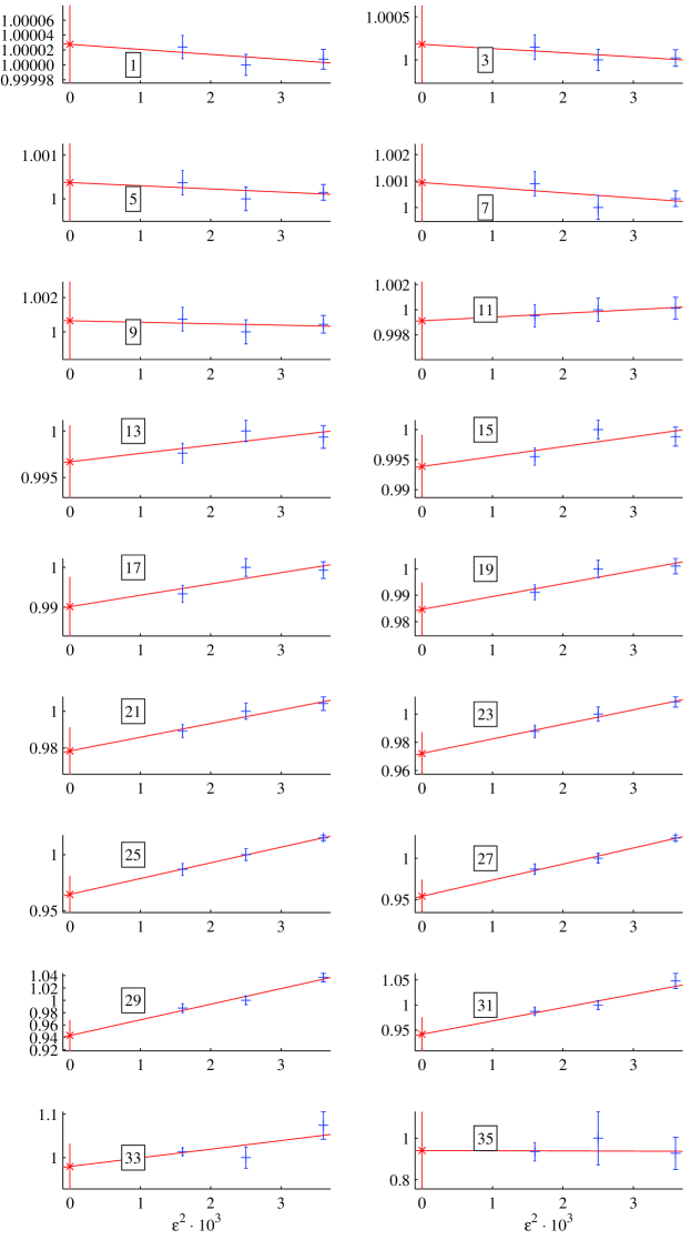
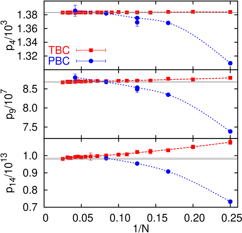
We show the $\epsilon^{2}\rightarrow 0$ extrapolation of the $N=28$ data in Fig. 1 for the example of odd orders $n+1$. For orders $n+1\leq 15$ no statistically significant slopes can be detected and the $\epsilon=0.05$ results are in perfect agreement within errors with the $\epsilon\rightarrow 0$ extrapolations. (One notable exception is the $\mathcal{O}(\alpha^{2})$ data, not depicted here.) For higher orders the non-vanishing size of $\epsilon$ introduces errors, which we estimate in the following way. From the $N=28$ data we compute the relative difference between the value of a coefficient $p_{n}$ obtained at the finite value $\epsilon=0.05$ and the extrapolated result:

$$d_{n}=\left|1-\frac{p_{n}(\epsilon=0)}{p_{n}(\epsilon=0.05)}\right|\,.$$ (10)

For all the volumes and orders where no $\epsilon\rightarrow 0$ extrapolation was carried out, we use $d_{n}p_{n}$ as the estimate of the uncertainty due to the non-zero time step. We then add $d_{n}p_{n}$ to the respective statistical error of $p_{n}$ obtained at $\epsilon=0.05$ in quadrature. For the coefficients $p_{n}(N)$ where the $\epsilon$-extrapolation has been carried out, we use the extrapolated value $p_{n}(N;\epsilon=0)$ and the associated error of the $\epsilon$-extrapolation instead.

Figure 2: The coefficients $p_{0}(N)$ (upper panel) and $p_{1}(N)$ (lower panel) for different linear lattice extents $N$, normalized with respect to the infinite volume expectations from diagrammatic perturbation theory. Circles denote the final values obtained either by increasing the respective errors (empty circles) or by extrapolating to $\epsilon=0$ (full circles) as detailed in the text. Squares correspond to the values obtained at the fixed time step $\epsilon=0.05$. For clarity the symbols have been shifted horizontally by different off-sets.

Figure 3: The coefficient $p_{19}(N)$ versus the linear lattice size $N$. The full circle denotes the $\epsilon=0$ extrapolated result, which at this order is only available for $N=28$. Open circles are the “final” values obtained by increasing the errors as detailed in the text, squares are the results obtained at a fixed time step $\epsilon=0.05$. The symbols have been shifted horizontally to enhance readability.

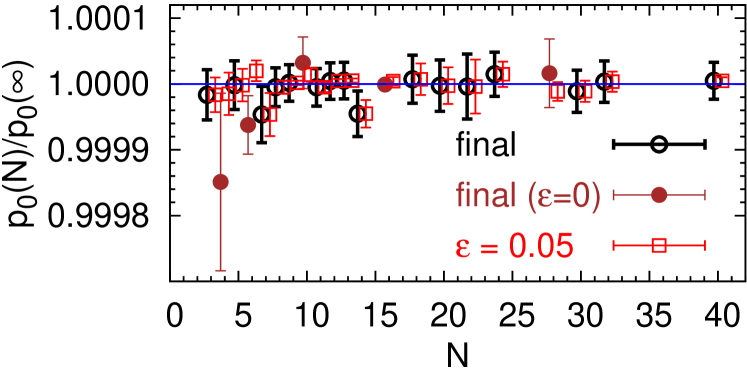
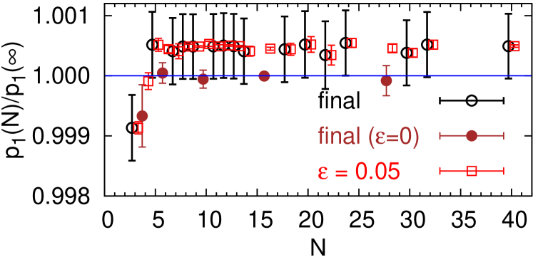
Figs. 2 and 3 show the impact of the $\epsilon$-extrapolation error on $p_{0,1,19}(N)$. In the upper panel of Fig. 2 we normalize the data to the analytically known value $p_{0}(\infty)=p_{0}(N)=4\pi/3$. We observe perfect agreement with this expectation. The $\epsilon$-extrapolation errors dominate for large volumes where the statistical errors are small. This is a general tendency for all orders $n$, but more pronounced for large $n$-values, see Fig. 3. In the lower panel of Fig. 2 we normalize the data to the known value $p_{1}(\infty)$. This plot further illustrates the quality of the $\epsilon$-extrapolation and that our error estimates are reasonable. Note that in this case a non-zero slope of the $\epsilon^{2}$-extrapolation was detected. For all but one of the volumes for which the extrapolation in $\epsilon^{2}$ was performed ($N=6,8,10,16,28$) we find perfect agreement within small errors with the infinite volume result. Only for $N=4$ are finite size effects significant. We also see how our procedure to estimate the $\epsilon$-extrapolation error (based on the deviation at $N=28$) correctly captures the systematics for all the volumes for which we could not perform an $\epsilon$-extrapolation.

Since the gauge action and the algorithm are local in spacetime and Langevin time one may expect the $\epsilon^{2}$-slopes to become independent of $N$ for sufficiently large lattice extents $N$, with $1/N^{2}$ corrections that will depend on the order of the expansion. Indeed, this expectation seems to be supported by our data, see Fig. 2, where the shifts between the $\epsilon=0.05$ and extrapolated data are similar in sign and magnitude for all volumes. However, in the present article we try to inject as little prejudice as possible into the analysis. Therefore, we follow the more conservative approach outlined above and abstain from using this information in the $\epsilon$-extrapolation.

II.3 Qualitative survey of PBC and TBC results

In our simulations we realize TBC. Numerically, these boundary conditions have the advantage of reduced statistical fluctuations and smaller autocorrelation times, due to the complete absence of zero momentum modes. Moreover, at small orders, these boundary conditions reduce finite size effects, and — as we shall see below — we can theoretically control TBC volume effects much better than PBC ones.

Figure 4: The coefficients $p_{4,9,14}(N)$ as functions of $1/N$ for the PBC Horsley:2012ra ; DiRenzo:2000ua (circles) and TBC (squares) data. The splines are drawn to guide the eye. The grey horizontal error bands are the infinite volume extrapolated values, see the last column of Table 4.

As detailed in Ref. Bali:2013pla , in addition to the TBC simulations presented here, for testing purposes and to enable comparison with literature values, we also performed simulations employing PBC. These PBC runs however were limited to small volumes and orders. Therefore, we will resort to literature values to enable a comparison between PBC and TBC. In Ref. Horsley:2012ra PBC results up to $\mathcal{O}(\alpha^{20})$ were presented for $N=4,6,8,12$. Up to $\mathcal{O}(\alpha^{10})$ these can be combined with earlier $N=8$ and $N=24$ results DiRenzo:2000ua , and up to $\mathcal{O}(\alpha^{3})$ with $N=32$ results DiRenzo:2004ge .

In Fig. 4, we compare the volume dependence of the PBC data from the literature with our TBC results for the examples of $p_{4}$, $p_{9}$ and $p_{14}$. The horizontal bands denote the infinite volume extrapolations and their errors, obtained as will be described in Sec. IV below and displayed in the last column of Table 4. These are independent of the boundary conditions and should be the same, irrespectively of using PBC or TBC. The PBC data appear to somewhat over-shoot the infinite volume values. It is not clear whether this behaviour can be attributed to a non-monotonous volume dependence or to a less well-controlled $\epsilon\rightarrow 0$ extrapolation of the PBC data, which were obtained using the unimproved $\mathcal{O}(\epsilon)$ Euler integration scheme. It is clear from the comparison that the TBC volume dependence is much reduced relative to the PBC case. However, at large orders also the TBC data start to show a significant dependence on $N$. In the next section, we will discuss theoretical expectations on the volume dependence both for TBC and for PBC.

III Finite volume corrections

In this section we determine the structure of the volume dependence of the coefficients $p_{n}(N)$ in the limit of large $N$. For simplicity we assume fixed aspect ratios between different directions, so that the finite volume effects can only depend on one parameter, $N$. More specifically, we simulate and consider symmetric lattice volumes. Together with the symmetry of the action, measure and observable under the interchange $a\leftrightarrow-a$, this implies that the coefficients $p_{n}(N)$ of Eq. (9) are functions of $N^{2}$ only:

$$p_{n}(N)=p_{n}-\frac{h_{n}(N)}{N^{2}}-\frac{f_{n}(N)}{N^{4}}-\frac{g_{n}(N)}{N^{6}}+\mathcal{O}\left(\frac{1}{N^{8}}\right)\,.$$ (11)

In the following, we will distinguish between TBC and PBC. Below we discuss theoretical expectations for the two types of boundary conditions, before we confront the numerical PBC data, where finite volume effects are more easily detectable, with different parametrizations.

III.1 Perturbative OPE with TBC

There are no zero modes using TBC (see, for instance Refs. Coste:1985mn ; Luscher:1985wf ) and perturbation theory is characterized by two distinct scales: $1/a$ and $1/(Na)\equiv 1/\ell$. In this context, the $N$-dependence of $h_{n}(N)$, $f_{n}(N)$ and $g_{n}(N)$ appears as the ratio of these two scales, $a/(Na)$, and perturbation theory predicts that it is logarithmic:

$$h_{n}(N)=\sum_{i=0}^{n}h_{n}^{(i)}\ln^{i}(N)\,,\quad f_{n}(N)=\sum_{i=0}^{n}f_{n}^{(i)}\ln^{i}(N)\,,\quad g_{n}(N)=\sum_{i=0}^{n}g_{n}^{(i)}\ln^{i}(N)\,.$$ (12)

We are interested in the large-$N$ (i.e. infinite volume) limit. In this situation

$$\frac{1}{a}\gg\frac{1}{Na}$$ (13)

and it makes sense to factorize the contributions of the different scales within the OPE framework. The hard modes, of scale $\sim 1/a$, determine the Wilson coefficients, whereas the soft modes, of scale $\sim 1/\ell$, can be described by expectation values of local gauge invariant operators. Due to the absence of such operators of dimension two, there can be no $1/N^{2}=a^{2}/\ell^{2}$ terms, i.e. $h_{n}=0$ in Eq. (11). The $1/N^{4}$-term, i.e. $f_{n}(N)$, is also fixed to a large extent by the OPE. The renormalization group invariant definition of the gluon condensate

$$\langle O_{\mathrm{G}}\rangle=-\frac{2}{\beta_{0}}\left\langle\Omega\left|\frac{\beta(\alpha)}{\alpha}G_{\mu\nu}^{c}G_{\mu\nu}^{c}\right|\Omega\right\rangle=\left\langle\Omega\left|\left[1+\mathcal{O}(\alpha)\right]\frac{\alpha}{\pi}G_{\mu\nu}^{c}G_{\mu\nu}^{c}\right|\Omega\right\rangle$$ (14)

is the only local gauge invariant expectation value of an operator of dimension $a^{-4}$. In the purely perturbative case discussed here, it only depends on the soft scale $1/\ell$, i.e. on the lattice size. On dimensional grounds, the perturbative gluon condensate $\langle O_{\mathrm{G}}\rangle_{\mathrm{soft}}$ is proportional to $1/\ell^{4}=1/(Na)^{4}$, and the logarithmic $\ell$-dependence is encoded in $\alpha(\ell^{-1})$. Therefore,

$$\frac{\pi^{2}}{36}\,a^{4}\langle O_{\mathrm{G}}\rangle_{\mathrm{soft}}=-\frac{1}{N^{4}}\sum_{n\geq 0}f_{n}\alpha^{n+1}((Na)^{-1})\,,$$ (15)

and the perturbative expansion of the plaquette on a finite volume of $N^{4}$ sites can be written as

$$\langle P\rangle_{\mathrm{pert}}(N)=P_{\mathrm{pert}}(\alpha)\langle\mathds{1}\rangle+\frac{\pi^{2}}{36}C_{\mathrm{G}}(\alpha)\,a^{4}\langle O_{\mathrm{G}}\rangle_{\mathrm{soft}}+\mathcal{O}\left(\frac{1}{N^{6}}\right)\,,$$ (16)

where

$$P_{\mathrm{pert}}(\alpha)=\sum_{n\geq 0}p_{n}\alpha^{n+1}$$ (17)

and $p_{n}$ are the infinite volume coefficients that we are interested in. The constant prefactor $\pi^{2}/36$ is chosen such that the Wilson coefficient, which only depends on $\alpha$, is normalized to unity for $\alpha=0$. It can be expanded as follows:

$$C_{\mathrm{G}}(\alpha) =1+\sum_{k\geq 0}c_{k}\alpha^{k+1}\,.$$ (18)

Combining the above three equations gives

$$\langle P\rangle_{\mathrm{pert}}(N) =\sum_{n\geq 0}\left[p_{n}-\frac{f_{n}(N)}{N^{4}}\right]\alpha^{n+1}$$ (19)

$$=\sum_{n\geq 0}p_{n}\alpha^{n+1}$$

$$\quad-\frac{1}{N^{4}}\left(1+\sum_{k\geq 0}c_{k}\alpha^{k+1}(a^{-1})\right)\times\sum_{n\geq 0}f_{n}\alpha^{n+1}((Na)^{-1})+\mathcal{O}\left(\frac{1}{N^{6}}\right)\,,$$

where ultimately we are interested in the $p_{n}$. Comparing the above expression with Eq. (12), we obtain $f_{n}^{(i)}$ as polynomials of $f_{j}$ and $c_{k}$:

$$f_{0}(N) =f_{0}\,,$$ (20)

$$f_{1}(N) =\left(f_{1}+c_{0}f_{0}\right)+f_{0}\frac{\beta_{0}}{2\pi}\ln(N)\,,$$ (21)

$$f_{2}(N) =\left(f_{2}+c_{0}f_{1}+c_{1}f_{0}\right)+\left[\left(2f_{1}+c_{0}f_{0}\right)\frac{\beta_{0}}{2\pi}+f_{0}\frac{\beta_{1}}{8\pi^{2}}\right]\ln(N)$$ (22)

$$+f_{0}\left(\frac{\beta_{0}}{2\pi}\right)^{\!\!2}\!\ln^{2}(N)\,,$$

$$f_{n}(N) =\left(f_{n}+c_{0}f_{n-1}+\cdots+c_{n-2}f_{1}+c_{n-1}f_{0}\right)$$ (23)

$$+\left\{\left[nf_{n-1}+(n-1)c_{0}f_{n-2}+(n-2)c_{1}f_{n-3}+\cdots+c_{n-2}f_{0}\right]\frac{\beta_{0}}{2\pi}+\cdots\right\}\ln(N)$$

$$+\cdots\,.$$

The $\beta$-function coefficients and the logarithms above are obtained by expanding $\alpha((Na)^{-1})$ within Eq. (19) in terms of $\alpha=\alpha(a^{-1})$ using the renormalization group, where we define the QCD $\beta$-function as

$$\beta(\alpha(\mu))=\frac{d\alpha(\mu)}{d\ln\mu}=-2\alpha\left[\beta_{0}\frac{\alpha(\mu)}{4\pi}+\beta_{1}\left(\frac{\alpha(\mu)}{4\pi}\right)^{2}+\cdots\right]\ ,$$ (24)

where

$$\beta_{0} =11\,,\quad\beta_{1}=102\,,$$

$$\quad\beta_{2}^{\overline{\mathrm{MS}}} =\frac{2857}{2}\,,\quad\beta_{2}^{\mathrm{latt}}=-6299.8999(6)\,,$$ (25)

$$\beta_{3}^{\overline{\mathrm{MS}}} \approx 29243.0\,,\quad\beta_{3}^{\mathrm{latt}}=-1.16(12)\times 10^{6}\,.$$

$\beta_{3}^{\overline{\mathrm{MS}}}$ was calculated in Ref. vanRitbergen:1997va where the previous results on $\beta_{0}$, $\beta_{1}$ and $\beta_{2}^{\overline{\mathrm{MS}}}$ are referenced. In the lattice scheme only $\beta_{2}^{\mathrm{latt}}$ has been computed diagrammatically Luscher:1995np ; Christou:1998ws ; Bode:2001uz . The value for $\beta_{3}^{\mathrm{latt}}$ that we quote Bali:2013qla was obtained by calculating the normalization of the heavy quark pole mass renormalon and then assuming the corresponding $\overline{\mathrm{MS}}$-scheme expansion to follow its asymptotic behaviour from orders $\alpha_{\mathrm{s}}^{4}$ onwards. Similar estimates, $\beta_{3}^{\mathrm{latt}}\approx-1.37\times 10^{6}$ up to $\beta_{3}^{\mathrm{latt}}\approx-1.55\times 10^{6}$, were found in Ref. Guagnelli:2002ia using a very different method.

Note that the coefficients $f_{n}^{(i)}$ within Eq. (12) for $i>0$ are entirely determined by $f_{j}$ and $\beta_{j}$ with $j<n$ and $c_{k}$ with $k<n-1$. Eqs. (19) – (23) are the most general parametrization of the $1/N^{4}$-effects for any lattice action using TBC.

Using the above conventions, the trace anomaly of the energy-momentum tensor reads

$$\langle\Omega|T_{\mu\mu}(0)|\Omega\rangle=\left\langle\Omega\left|\frac{\beta(\alpha)}{4\alpha}G_{\mu\nu}^{c}(0)G_{\mu\nu}^{c}(0)\right|\Omega\right\rangle=-\frac{\beta_{0}}{8}\langle O_{\mathrm{G}}\rangle\,,$$ (26)

which in turn equals the expectation value of the Lagrangian density times $\beta(\alpha)/\alpha$. In this paper we employ the Wilson action, for which the discretized Lagrangian is exactly proportional to the plaquette $P$, see Eq. (7), so that the above relation — in this case between the plaquette and $a^{4}\langle O_{\mathrm{G}}\rangle$ — holds up to $\mathcal{O}(a^{6})$ corrections. This fixes the Wilson coefficient exactly DiGiacomo:1990gy ; DiGiacomo:1989id :

$$C_{\mathrm{G}}(\alpha) =1+\sum_{k\geq 0}c_{k}\alpha^{k+1}=-\frac{\beta_{0}\alpha^{2}}{2\pi\beta(\alpha)}$$ (27)

$$=1-\frac{\beta_{1}}{\beta_{0}}\frac{\alpha}{4\pi}+\frac{\beta_{1}^{2}-\beta_{0}\beta_{2}}{\beta_{0}^{2}}\left(\frac{\alpha}{4\pi}\right)^{2}-\frac{\beta_{1}^{3}-2\beta_{0}\beta_{1}\beta_{2}+\beta_{0}^{2}\beta_{3}}{\beta_{0}^{3}}\left(\frac{\alpha}{4\pi}\right)^{3}+\mathcal{O}(\alpha^{4})\,.$$

Note that $C_{\mathrm{G}}(\alpha)$ is scheme-dependent not only through $\alpha$, but also explicitly, due to its dependence on the higher $\beta$-function coefficients $\beta_{2}$ etc.. The $c_{k}$ depend on the $\beta_{i}$ with $i\leq k+1$ via Eq. (27).

Finally, we consider $1/N^{6}$-effects. At this order the number of terms and thus fit parameters grows quite rapidly. Therefore, we do not attempt a complete study of the $1/N^{6}$ corrections, but aim at achieving a qualitative understanding of the corresponding structure. The philosophy is the same as above: we have to carry out the OPE program to the next order. This means that we have to consider all gauge invariant local operators of dimension six that are singlets under the hypercubic subgroup H(4) of O(4). Three such operators exist Luscher:1984xn , one of which can be eliminated via the equations of motion for on-shell quantities. We consider the O(4) invariant $\langle O_{6}\rangle=\langle gG^{3}\rangle$ as one such example but in principle a second matrix element needs to be added. $O_{6}$ has a non-trivial anomalous dimension, complicating the logarithmic corrections. The contribution of this term will be

$$\delta\langle P\rangle_{\mathrm{pert}}(N) \sim\frac{1}{N^{6}}\left[1+\sum_{k\geq 0}c^{(6)}_{k}\alpha^{k+1}(a^{-1})\right]\times\exp\left[\int_{\alpha(a^{-1})}^{\alpha((Na)^{-1})}\frac{d\alpha^{\prime}}{\alpha^{\prime}}\left(\gamma_{0}+\gamma_{1}\alpha^{\prime}+\cdots\right)\right]$$

$$\quad\times\sum_{n\geq 0}g_{n}\alpha^{n+1}((Na)^{-1})\,.$$ (28)

$\gamma_{0}$, the one-loop anomalous dimension of $O_{6}$, is known Narison:1983kn but not the higher orders in the scheme we use. The above structure results in three new unknown parameters for each additional power of $\alpha$: one additional $c_{k}^{(6)}$-value for the Wilson coefficient, one higher order anomalous dimension coefficient $\gamma_{j}$ and an additional $g_{n}$-value from the expansion of $\langle O_{6}\rangle_{\mathrm{soft}}$.

Besides the OPE of the plaquette expectation value, we also have to perform the OPE of the lattice action, to obtain an effective action where only soft modes remain dynamical:

$$S=\frac{1}{4}\int\!d^{4}\!x\,G^{2}(x)+a^{2}C_{6}(a^{-1})\int\!d^{4}\!x\,gG^{3}(x)+\cdots\,.$$ (29)

The dimension six operators here are the same as those considered above, since the symmetries are the same. Again we focus on $O_{6}$, which produces the following additional contribution to $P_{\mathrm{pert}}(N)$:

$$\tilde{\delta}\langle P\rangle_{\mathrm{pert}}(N) \sim a^{6}C_{6}(a^{-1})\,\int\!d^{4}\!y\,\langle\mathcal{T}\!\left\{G^{2}(0),O_{6}(y)\right\}\rangle_{\mathrm{soft}}$$ (30)

$$\sim\frac{1}{N^{6}}\left[1+\sum_{k\geq 0}\tilde{c}^{(6)}_{k}\alpha^{k+1}(a^{-1})\right]\times\exp\left[\int_{\alpha}^{\alpha((Na)^{-1})}\frac{d\alpha^{\prime}}{\alpha^{\prime}}\left(\gamma_{0}+\gamma_{1}\alpha^{\prime}+\cdots\right)\right]$$

$$\times\sum_{n\geq 0}\tilde{g}_{n}\alpha^{n+1}((Na)^{-1})\,.$$

The anomalous dimension is the same as that in Eq. (28), as the operator is the same. Since we employ the plaquette action, also the Wilson coefficient is identical to that in Eq. (28) ($\tilde{c}^{(6)}_{k}={c}^{(6)}_{k}$) and differences between the soft matrix elements can be absorbed into Eq. (28), redefining $g_{n}+\tilde{g}_{n}\mapsto g_{n}$. Therefore, no additional parameters are required. The same arguments also apply to the second independent operator of dimension six. Overall, at $\mathcal{O}(1/N^{6})$ we expect a total of six new parameters per order in $\alpha$, which exceeds our fitting capabilities. Therefore, we do not attempt a more systematic study of the $1/N^{6}$-effects.

III.2 Non-perturbative OPE with TBC

Since in NSPT we Taylor expand in powers of $g$ before averaging over the gauge variables, no mass gap is generated dynamically. It is interesting though to discuss in what particular setting our results can be related to non-perturbative results obtained by Monte-Carlo lattice simulations. In this case an additional scale, $\Lambda_{\mathrm{QCD}}\sim 1/a\,e^{-2\pi/(\beta_{0}\alpha)}$, is generated dynamically. However, we can always tune $N$ and $\alpha$ such that

$$\frac{1}{a}\gg\frac{1}{Na}=\frac{1}{\ell}\gg\Lambda_{\mathrm{QCD}}\,.$$ (31)

In this small-volume situation we encounter a double expansion in powers of $a/\ell$ and $a\Lambda_{\mathrm{QCD}}$ (or $(\ell\Lambda_{\mathrm{QCD}})(a/\ell)$). The construction of the OPE is completely analogous to that of Sec. III.1 above and we obtain

$$\langle P\rangle_{\mathrm{MC}} =\frac{1}{Z}\left.\int\![dU_{x,\mu}]\,e^{-S[U]}P[U]\right|_{\mathrm{MC}}$$ (32)

$$=P_{\mathrm{pert}}(\alpha)\langle\mathds{1}\rangle+\frac{\pi^{2}}{36}C_{\mathrm{G}}(\alpha)\,a^{4}\langle O_{\mathrm{G}}\rangle_{\mathrm{MC}}+\mathcal{O}\left(a^{6}\right)\,.$$

In the last equality we have factored out the hard scale, $1/a$, from the scales $1/(Na)$ and $\Lambda_{\mathrm{QCD}}$, which are encoded in $\langle O_{\mathrm{G}}\rangle_{\mathrm{MC}}$. Exploiting the right-most inequality of Eq. (31), we can expand $\langle O_{\mathrm{G}}\rangle_{\mathrm{MC}}$ as follows:

$$\langle O_{\mathrm{G}}\rangle_{\mathrm{MC}}=\langle O_{\mathrm{G}}\rangle_{\mathrm{soft}}\left[1+\mathcal{O}(\Lambda_{\mathrm{QCD}}^{2}\ell^{2})\right]\,.$$ (33)

Hence, a non-perturbative small-volume simulation would yield the same expression as NSPT, up to non-perturbative corrections that can be made arbitrarily small by reducing $a$ and therefore $\ell=Na$, keeping $N$ fixed. In other words, $p_{n}^{\mathrm{NSPT}}(N)=p_{n}^{\mathrm{MC}}(N)$ up to non-perturbative corrections.

We can also consider the limit

$$\frac{1}{a}\gg\Lambda_{\mathrm{QCD}}\gg\frac{1}{Na}\,.$$ (34)

This is the standard situation realized in non-perturbative lattice simulations. Again the OPE can be constructed as in Sec. III.1 and Eq. (32) also holds. The difference is that now

$$\langle O_{\mathrm{G}}\rangle_{\mathrm{MC}}=\langle O_{\mathrm{G}}\rangle_{\mathrm{NP}}\left[1+\mathcal{O}\left(\frac{1}{\Lambda_{\mathrm{QCD}}^{2}\ell^{2}}\right)\right]\,,$$ (35)

where $\langle O_{\mathrm{G}}\rangle_{\mathrm{NP}}\sim\Lambda_{\mathrm{QCD}}^{4}$ is the so-called non-perturbative gluon condensate introduced in Ref. Vainshtein:1978wd .

Finally, we re-emphasize that Eq. (32) holds, irrespectively of ordering the scales according to Eq. (31) or to Eq. (34). We further remark that the relation Eq. (27) for the Wilson coefficient $C_{\mathrm{G}}$ for the plaquette action also holds when non-perturbative effects are included.

III.3 Perturbative and non-perturbative OPEs with PBC

In the case of PBC one encounters constant, i.e. zero, modes. The effects associated to these are non-perturbative in nature. They can be interpreted as introducing an extra scale $g^{1/2}/(Na)$, besides the perturbative scales $1/a$ and $1/(Na)$. Therefore, with PBC, irrespectively of how small the coupling is, there are non-perturbative effects associated with these modes, which will invalidate the perturbative OPE of the plaquette with PBC. The violations of the perturbative OPE will decrease with $1/N^{4}$ because the relative measure of the zero mode contributions becomes suppressed by this factor for large volumes. These effects are then of the same order as those associated with $\langle O_{\mathrm{G}}\rangle_{\mathrm{soft}}$. Both contributions will undergo mixing and invalidate the parametrization of the finite size effects Eqs. (19) – (23).

The $\mathcal{O}(\alpha)$ zero mode contribution has been explicitly computed in Ref. Coste:1985mn . Generalizing this derivation to higher orders in $\alpha$ becomes extremely complicated. In particular one has to disentangle the contributions of the different scales. Since it is not clear how to properly account for the zero modes, in practice they are omitted in diagrammatic PBC calculations or subtracted in NSPT computations. In particular, the literature results of $p_{n}^{\mathrm{PBC}}(N)$ that we use here do not include these contributions. Therefore, these literature values do not correspond to any physical situation, except in the infinite volume limit where zero modes can be neglected. In other words, the coefficients $p_{n}^{\mathrm{PBC}}(N)$ cannot be obtained from a fit to non-perturbative data (with infinite precision) of the plaquette computed in the situation

$$\frac{1}{a}\gg\frac{1}{Na}\gg\frac{g^{1/2}}{Na}\gg\Lambda_{\mathrm{QCD}}\,.$$ (36)

This means that one cannot apply the standard OPE and the finite size behaviour of the $p_{n}^{\mathrm{PBC}}(N)$ is less well constrained than in the TBC case. However, the leading-order corrections will still scale as $1/N^{4}$, and they will be logarithmically modulated. Given precise data and large volumes, this may still suffice to extrapolate high-order coefficients $p_{n}(N)$ to infinite $N$.

III.4 Phenomenological fits to PBC data

In order to confirm the validity of the interpolating function and the perturbative OPE structure discussed above, we perform a series of tests using the PBC data. In particular we investigate numerically whether any $1/N^{2}$ effects, which are incompatible with the expected OPE structure, may nevertheless be present in the data or in diagrammatic lattice perturbation theory.

We start by studying the low-order coefficients obtained using diagrammatic lattice perturbation theory. At $\mathcal{O}(\alpha)$ exact results can be derived both for PBC and for TBC:

$$p^{\mathrm{TBC}}_{0}(N)=\frac{4}{3}\pi\,,\qquad p^{\mathrm{PBC}}_{0}(N)=\frac{4}{3}\pi\left(1-\frac{1}{N^{4}}\right)\,.$$ (37)

One consequence of using TBC instead of PBC is that the one-loop behaviour is flat: $p_{0}^{\mathrm{TBC}}\left(N\right)=p\left(\infty\right)\equiv p_{0}$. In Fig. 2 we compared our TBC $p_{0}\left(N\right)$ data with the analytical value and found agreement within errors down to the smallest lattice volume, so finite volume effects are truly absent at leading order.

The $\mathcal{O}(\alpha^{2})$ infinite volume coefficient was first computed in Ref. DiGiacomo:1981wt and with increased precision in Ref. Alles:1998is . We have recomputed it using the formulae of this last reference together with the very precise lattice integrals of Ref. Luscher:1995np , obtaining

$$p_{1}=5.355009398(6)\,.$$ (38)

In order to study the $N$-dependence we have also computed $p^{\mathrm{PBC}}_{1}(N)$ for $N\leq 64$ and high precision, using the formulae given in Ref. Heller:1984hx . From this analysis we conclude that to this order there are no $1/N^{2}$ effects and we obtain

$$p^{\mathrm{PBC}}_{1}(N)\approx p_{1}-\frac{1}{N^{4}}\left[3.3\ln(N)+13.4\right]-\frac{18}{N^{6}}\,,$$ (39)

where we have fixed the $p_{1}$-value to Eq. (38).

Comparing Eqs. (39) and (37) with Eq. (21), we observe that the coefficient of $\ln(N)$ does not comply with the OPE ($3.3\neq\beta_{0}f_{0}=22/3$). This difference illustrates that we cannot use the OPE with PBC after subtracting the zero modes. The zero modes contribute to the $\mathcal{O}(\alpha)$ constant as well as to the logarithmic and constant terms at $\mathcal{O}(\alpha^{2})$ (at higher orders the contribution could be more complicated, due to the $g^{1/2}/(Na)$ scale):

$$\delta p^{\mathrm{zero\;mode}}_{1}(N)=\frac{1}{N^{4}}\left[a\ln(N)+b\right]+\mathcal{O}\left(\frac{1}{N^{6}}\right)\,.$$ (40)

This term was partially subtracted by omitting zero momentum contributions to the lattice sums. In any case, at present nothing about the coefficients $a$ or $b$ is known. Based on this diagrammatic perturbation theory analysis for PBC we conclude that there are no $1/N^{2}$ effects at $\mathcal{O}(\alpha)$ nor at $\mathcal{O}(\alpha^{2})$. We remark that there are indications that these may also be absent at $\mathcal{O}(\alpha^{3})$, for which the infinite volume coefficient was first computed in Ref. Alles:1993dn and with increased precision in Ref. Alles:1998is :

$$p_{2}=27.1983(9)\,.$$ (41)

We now turn to the NSPT PBC data. These cover orders up to $\alpha^{20}$. We have seen in Sec. II.3 (see Fig. 4) that the dependence on $1/N$ is much more pronounced with PBC than with TBC. While this additionally complicates the infinite volume extrapolation of PBC results, it allows us to identify the power scaling of the leading $1/N$ correction with higher numerical significance than for TBC.

Table 2: Exploratory fits to PBC data and the resulting $\chi^{2}_{\mathrm{red}}$ as a measure of the fit quality. All fits have two parameters per order $n$. The finite size correction is $f_{n}(N)/N^{d}$. The second column is for $f_{n}(N)$ with renormalization group running while the third column is for constant $f_{n}(N)=f_{n}$.
 

$\mathrm{power}\,\,d{}{}$	$\chi^{2}_{\mathrm{red}}\,\,(\mathrm{run})$	$\chi^{2}_{\mathrm{red}}\,\,(\mathrm{no\,\,run})$
$2$	$63.40$	$20.19$
$4$	$4.24$	$7.45$
$6$	$11.01$	$22.79$

We attempt several fits to PBC $N\geq 4$ data, assuming the leading term to be of the form $p_{n}-f_{n}(N)/N^{d}$ with $d=2,4,6$, where we allow for two different parametrization of $f_{n}(N)$: $f_{n}(N)=\mbox{const.}=f_{n}$ (no run), and $f_{n}(N)$ as given in Eqs. (20) – (23) (run), setting $c_{n}=0$. In each of these parametrizations we encounter two fit parameters, $p_{n}$ and $f_{n}$, per order of the expansion. The resulting reduced $\chi^{2}$-values $\chi^{2}_{\mathrm{red}}\equiv\chi^{2}/N_{\rm DF}$ (as a measure of the quality of the respective fits) are shown in the second and third columns of Table 2. The numbers indicate that the parametrizations work best for $d\sim 4$. Higher and, most notably, lower values of $d$ are clearly ruled out by the data, irrespectively of including a running into the $f_{n}(N)$ or not. We also see that for $d=4$ the data prefer “running” to “no running”. However, we have neglected the Wilson coefficient of the gluon condensate (the $c_{k}$), ignored the (unknown) effect of the subtracted zero modes and most of the literature data are available only for rather small $N$ ($=4,6,8$ and 12). Therefore, it is not surprising that the value $\chi^{2}_{\mathrm{red}}\approx 4.2$ in the best “running” $d=4$ case is still unsatisfactory. The number of parameters needed to incorporate these effects into the parametrization will quickly explode with the order, turning a model-independent fit to PBC data impossible for any realistic number of volumes.

We conclude that no $1/N^{2}$ terms exist and that some sort of running of the $1/N^{4}$-term is required to describe the PBC data. We take this as a confirmation of the theoretical arguments presented in Sec. III.1.

IV Infinite volume coefficients

In this section we determine the infinite volume coefficients $p_{n}$, defined in Eq. (11), for $0<n\leq 34$. For $n=0$, we use the exact result $p_{0}=4\pi/3$. Our default fit function for $p_{n}(N)$ is (see also Eq. (19))

$$p_{n}(N)=p_{n}-\frac{f_{n}(N)}{N^{4}}\,,$$ (42)

where the $f_{n}(N)$ are defined in Eqs. (20) – (23). $p_{n}(N)$ depends on the fit parameters $p_{n}$, $f_{j}$ with $j\leq n$, and $c_{k}$, with $k\leq n-1$. We know from diagrammatic calculations that $f_{0}=0$. Since $f_{0}=0$, $c_{33}$ does not appear in the fit. We will also set $c_{32}=0$, as this coefficient cannot be parametrically distinguished from $f_{34}$. For the $\beta$-function coefficients that appear in our fit function, we will set $\beta_{0}$, $\beta_{1}$ and $\beta_{2}$ to their known values Eq. (25) (note that $\beta_{2}$ depends on the scheme) and $\beta_{i}=0$ for $i\geq 3$. We also fix $c_{0}$ and $c_{1}$ to their known values of Eq. (27) ($c_{1}$ is scheme-dependent too). Therefore, our default fit function depends on a total of 34 $p_{n}$-coefficients, 34 $f_{n}$-coefficients, and 30 $c_{n}$-coefficients. This function with 98 free parameters should describe all 35 orders of perturbation theory on the volumes listed in Table 1 for any $N$ bigger than a small volume cut-off $\nu\leq N$. 15 different volumes will contribute to our primary fit, described below.

The combined dependence on $f_{j}$ and $c_{k}$ introduces strong correlations between different orders, which we take into account by simultaneously fitting all $p_{n}(N)$ for $0<n\leq 34$. Unlike in Ref. Bali:2013pla , we cannot, in a first sweep, fit each new $p_{n}(N)$ independently with two new fit parameters $f_{n}$ and $c_{n-1}$, keeping the $f_{j}$- and $c_{k}$-values that were obtained at previous orders $k<j<n$ fixed and, subsequently, run the fit to convergence. The reason is that the $c_{k}$ non-linearly couple different orders, which considerably complicates the fitting procedure. Particularly problematic is the introduction of the $c_{k}$ for small values of $k$, which makes finding stable solutions quite difficult (with a large region of the parameter space of $c_{k}$ and $f_{j}$ producing small variations of $\chi^{2}_{\mathrm{red}}$). This is so because the parametrization cannot easily distinguish between, for instance, $c_{0}f_{33}\alpha(a^{-1})\alpha^{34}((Na)^{-1})$ and $f_{34}\alpha^{35}((Na)^{-1})$, as the running of these two terms is very similar. This problem is alleviated because we know $c_{0}$ and $c_{1}$ analytically. Fortunately, as we increase the order $k$ of $c_{k}$ the running of different products $c_{k}f_{n-k}\alpha^{n}(a^{-1})\alpha^{n-k+1}((Na)^{-1})$ becomes more and more distinguishable.

Table 3: $\chi^{2}_{\mathrm{red}}$ and $p_{n}$ for different values of $\nu$ using the fit function Eq. (42). The $n=0$ values were fixed to the exact result. The diagrammatic expectations are $p_{1}=5.355009398(6)$ and $p_{2}=27.1983(9)$. 

$\nu$	$13$	$11$	$9$	$7$
$\chi^{2}_{\mathrm{red}}$	$0.826107$	$0.768641$	$0.700803$	$0.863024$
$p_{0}$	$\mathbf{4{\boldsymbol{\pi}}/3}$	$\mathbf{4{\boldsymbol{\pi}}/3}$	$\mathbf{4{\boldsymbol{\pi}}/3}$	$\mathbf{4{\boldsymbol{\pi}}/3}$
$p_{1}$	$5.35606(66)$	$5.35539(25)$	$5.35522(13)$	$5.35509(12)$
$p_{2}/10$	$2.71947(22)$	$2.71978(14)$	$2.719761(94)$	$2.719752(81)$
$p_{3}/10^{2}$	$1.80963(13)$	$1.809690(92)$	$1.809718(73)$	$1.809747(64)$
$p_{4}/10^{3}$	$1.38319(23)$	$1.38324(14)$	$1.383242(90)$	$1.383285(75)$
$p_{5}/10^{4}$	$1.15170(53)$	$1.15189(42)$	$1.15184(26)$	$1.15186(12)$
$p_{6}/10^{5}$	$1.01632(63)$	$1.01650(52)$	$1.01678(35)$	$1.01670(16)$
$p_{7}/10^{5}$	$9.3553(64)$	$9.3572(54)$	$9.3605(40)$	$9.3621(21)$
$p_{8}/10^{6}$	$8.8936(53)$	$8.8949(44)$	$8.8971(35)$	$8.9025(23)$
$p_{9}/10^{7}$	$8.6745(43)$	$8.6752(39)$	$8.6803(29)$	$8.6858(27)$
$p_{10}/10^{8}$	$8.6358(74)$	$8.6370(67)$	$8.6441(53)$	$8.6532(45)$
$p_{11}/10^{9}$	$8.744(14)$	$8.745(12)$	$8.7568(97)$	$8.7706(74)$
$p_{12}/10^{10}$	$8.977(25)$	$8.979(20)$	$8.993(16)$	$9.003(14)$
$p_{13}/10^{11}$	$9.331(38)$	$9.331(30)$	$9.350(23)$	$9.366(19)$
$p_{14}/10^{12}$	$9.805(54)$	$9.796(43)$	$9.827(33)$	$9.847(28)$
$p_{15}/10^{14}$	$1.0397(78)$	$1.0382(63)$	$1.0423(46)$	$1.0448(39)$
$p_{16}/10^{15}$	$1.111(12)$	$1.110(10)$	$1.1143(69)$	$1.1173(57)$
$p_{17}/10^{16}$	$1.196(19)$	$1.194(16)$	$1.201(10)$	$1.2041(84)$
$p_{18}/10^{17}$	$1.294(29)$	$1.294(26)$	$1.303(15)$	$1.307(12)$
$p_{19}/10^{18}$	$1.409(44)$	$1.416(39)$	$1.421(22)$	$1.426(18)$
$p_{20}/10^{19}$	$1.544(64)$	$1.554(57)$	$1.562(32)$	$1.567(25)$
$p_{21}/10^{20}$	$1.704(93)$	$1.723(82)$	$1.727(44)$	$1.731(35)$
$p_{22}/10^{21}$	$1.89(13)$	$1.93(12)$	$1.924(61)$	$1.922(48)$
$p_{23}/10^{22}$	$2.11(19)$	$2.20(16)$	$2.160(84)$	$2.143(69)$
$p_{24}/10^{23}$	$2.38(28)$	$2.54(23)$	$2.45(12)$	$2.40(10)$
$p_{25}/10^{24}$	$2.76(40)$	$3.02(33)$	$2.82(18)$	$2.71(15)$
$p_{26}/10^{25}$	$3.31(58)$	$3.71(50)$	$3.32(28)$	$3.10(24)$
$p_{27}/10^{26}$	$4.14(85)$	$4.79(87)$	$4.04(46)$	$3.60(40)$
$p_{28}/10^{27}$	$5.4(13)$	$6.6(17)$	$5.15(82)$	$4.32(67)$
$p_{29}/10^{28}$	$7.6(22)$	$9.6(33)$	$7.0(15)$	$5.5(11)$
$p_{30}/10^{30}$	$1.20(43)$	$1.55(67)$	$1.04(29)$	$0.76(21)$
$p_{31}/10^{31}$	$1.90(84)$	$2.5(13)$	$1.64(55)$	$1.15(38)$
$p_{32}/10^{32}$	$3.1(17)$	$4.3(26)$	$2.7(11)$	$1.90(70)$
$p_{33}/10^{33}$	$5.2(33)$	$7.3(52)$	$4.8(20)$	$3.3(14)$
$p_{34}/10^{34}$	$9.1(65)$	$13(10)$	$8.8(40)$	$6.4(27)$

Table 4: The same as Table 3. $\nu=9$, except for the first column: adding the $1/N^{6}$-term (Eq. (43)) and setting $\nu=8$. Second column: including $\beta_{3}^{\mathrm{latt}}$ of Eq. (25). Third column: setting $\beta_{2}^{\mathrm{latt}}=0$. Last column: result of Table 3, including systematic errors.

	$1/N^{6}$	$\beta_{3}\neq 0$	$\beta_{2}=0$	$\mathrm{Final\;result}$
$\chi^{2}_{\mathrm{red}}$	$0.671138$	$0.70238$	$0.70026$
$p_{0}$	$\mathbf{4{\boldsymbol{\pi}}/3}$	$\mathbf{4{\boldsymbol{\pi}}/3}$	$\mathbf{4{\boldsymbol{\pi}}/3}$	$\mathbf{4{\boldsymbol{\pi}}/3}$
$p_{1}$	$5.35559(23)$	$5.35522(13)$	$5.35522(13)$	$5.35522(18)$
$p_{2}/10$	$2.71974(14)$	$2.719762(94)$	$2.719761(94)$	$2.719761(95)$
$p_{3}/10^{2}$	$1.80966(10)$	$1.809719(73)$	$1.809718(73)$	$1.809718(78)$
$p_{4}/10^{3}$	$1.38317(15)$	$1.383248(90)$	$1.383244(90)$	$1.38324(10)$
$p_{5}/10^{4}$	$1.15152(45)$	$1.15164(11)$	$1.15184(26)$	$1.15184(26)$
$p_{6}/10^{5}$	$1.01617(55)$	$1.01694(32)$	$1.01677(35)$	$1.01678(36)$
$p_{7}/10^{5}$	$9.3553(55)$	$9.3620(38)$	$9.3604(40)$	$9.3605(43)$
$p_{8}/10^{6}$	$8.8924(44)$	$8.8978(34)$	$8.8970(35)$	$8.8971(65)$
$p_{9}/10^{7}$	$8.6729(34)$	$8.6800(27)$	$8.6803(29)$	$8.6803(62)$
$p_{10}/10^{8}$	$8.6331(61)$	$8.6425(50)$	$8.6440(53)$	$8.644(11)$
$p_{11}/10^{9}$	$8.741(11)$	$8.759(10)$	$8.7565(97)$	$8.757(17)$
$p_{12}/10^{10}$	$8.980(19)$	$8.998(15)$	$8.992(16)$	$8.993(19)$
$p_{13}/10^{11}$	$9.339(30)$	$9.355(22)$	$9.350(23)$	$9.350(28)$
$p_{14}/10^{12}$	$9.819(45)$	$9.833(31)$	$9.827(33)$	$9.827(38)$
$p_{15}/10^{14}$	$1.0424(65)$	$1.0427(45)$	$1.0422(47)$	$1.0423(53)$
$p_{16}/10^{15}$	$1.1162(95)$	$1.1150(64)$	$1.1143(69)$	$1.1143(75)$
$p_{17}/10^{16}$	$1.204(14)$	$1.2024(91)$	$1.201(10)$	$1.201(11)$
$p_{18}/10^{17}$	$1.309(20)$	$1.305(13)$	$1.303(15)$	$1.303(16)$
$p_{19}/10^{18}$	$1.433(28)$	$1.424(20)$	$1.421(22)$	$1.421(23)$
$p_{20}/10^{19}$	$1.579(39)$	$1.565(28)$	$1.562(32)$	$1.562(32)$
$p_{21}/10^{20}$	$1.745(56)$	$1.727(41)$	$1.727(45)$	$1.727(44)$
$p_{22}/10^{21}$	$1.955(81)$	$1.921(56)$	$1.924(62)$	$1.924(61)$
$p_{23}/10^{22}$	$2.21(12)$	$2.155(77)$	$2.160(86)$	$2.160(86)$
$p_{24}/10^{23}$	$2.55(19)$	$2.44(11)$	$2.45(12)$	$2.45(13)$
$p_{25}/10^{24}$	$3.02(31)$	$2.80(16)$	$2.83(18)$	$2.82(21)$
$p_{26}/10^{25}$	$3.71(50)$	$3.26(23)$	$3.33(28)$	$3.32(35)$
$p_{27}/10^{26}$	$4.78(84)$	$3.92(37)$	$4.06(47)$	$4.04(63)$
$p_{28}/10^{27}$	$6.6(15)$	$4.92(63)$	$5.19(83)$	$5.15(12)$
$p_{29}/10^{28}$	$9.7(26)$	$6.6(11)$	$7.1(15)$	$7.0(22)$
$p_{30}/10^{30}$	$1.57(47)$	$9.6(21)$	$1.05(29)$	$1.04(40)$
$p_{31}/10^{31}$	$2.60(87)$	$1.49(40)$	$1.66(56)$	$1.64(74)$
$p_{32}/10^{32}$	$4.4(16)$	$2.46(76)$	$2.8(11)$	$2.7(13)$
$p_{33}/10^{33}$	$7.6(30)$	$4.2(15)$	$4.9(21)$	$4.8(25)$
$p_{34}/10^{34}$	$13.6(55)$	$7.7(29)$	$9.0(41)$	$8.8(46)$

Using the setup described above, we fit to subsets of data constrained by $N\geq\nu$, and vary $\nu$. We display some of these results in Table 3 and use them to explore the validity range of Eq. (42). Our “thermometer” for this will be to obtain acceptable $\chi^{2}_{\mathrm{red}}$-values and agreement with $p_{1}$ and $p_{2}$ from diagrammatic lattice perturbation theory. We find that including small volumes improves the quality of the fit down to a cut-off $\nu=9$. For smaller values of $\nu$ the $\chi^{2}_{\mathrm{red}}$-values rapidly increase. This we interpret as becoming sensitive to higher order finite volume effects that are not accounted for in our parametrization. Therefore, we take the results from the $\nu=9$ fit, which uses 365 data points, as our central values.

We now estimate the systematic errors. They are due to our incomplete parametrization of the finite volume corrections, since we have set higher $\beta$-function coefficients to zero within the $1/N^{4}$ terms. Moreover, we have ignored $1/N^{6}$- and higher order finite volume corrections.

We determine the $\mathcal{O}(1/N^{4})$ truncation uncertainties in two ways. First we consider the differences between the central values of the $\nu=9$ and $\nu=7$ fits shown in Table 3. The other possibility we explore is varying the parametrization to check the robustness of our results. In principle, the leading parametric uncertainty originates from the omission of the higher order $\beta$-function coefficients: $\beta_{3}$, $\beta_{4}$, etc., which affect the log-structure of the $1/N^{4}$ corrections. Therefore, we perform alternative fits either eliminating $\beta_{2}$ (we also set $\beta_{2}=0$ in $c_{1}$) or incorporating $\beta_{3}^{\mathrm{latt}}$ (quoted in Eq. (25)) into our fits. For the first case the outcome is given in the third column of Table 4. We observe that the shifts are much smaller than the statistical errors or the differences between the $\nu=9$ and $\nu=7$ results. Including $\beta_{3}^{\mathrm{latt}}$ means including the associated $\ln(N)$ running and fixing $c_{2}$ to its value Eq. (27). We display this result in the second column of Table 4. The shifts of the $p_{n}$ are well below the statistical errors, even at high orders. It is worth mentioning that the bulk of the changes is produced by fixing $c_{1}$ or $c_{2}$ to the values Eq. (27), while the different running is a subleading effect. This explains why fixing $\beta_{2}=0$ had little impact on the $p_{n}$-values: the $c_{k}$ ($k>1$) were kept as fit parameters. Since the differences between truncating at $\beta_{1}$-, $\beta_{2}$- or $\beta_{3}$-order (see Table 4) can clearly be neglected, we take the differences between the results of the $\nu=9$ and $\nu=7$ fits displayed in Table 3 as our systematic uncertainties and add these in quadrature to the statistical errors of our parameters from the primary $\nu=9$ fit. The final results are shown in the last column of Table 4. All results from fits with acceptable $\chi^{2}_{\mathrm{red}}$-values that we performed, including those displayed in the two tables, perfectly agree within errors with these final results.

The above error analysis is quite similar to the one we did for the expansion of the Polyakov line in Ref. Bali:2013pla . In that case the systematic errors were dominant, and could mainly be attributed to omitting higher $\beta$-function coefficients. For the plaquette expansion the situation is quite different: the systematic uncertainties are of the same size as the statistical errors and are not dominated by the impact of omitting higher $\beta$-function coefficients.

The main parametric uncertainty in our case are $1/N^{6}$-effects. Their significance should rapidly diminish as the volume cut-off $\nu$ is increased. Therefore, the systematic errors estimated above by varying $\nu$ should also account for the truncation of the parametrization at $\mathcal{O}(1/N^{4})$. We will now check this assumption by adding $1/N^{6}$ corrections. As discussed in Sec. III.1, we cannot include the most general $\mathcal{O}(1/N^{6})$ expression compatible with the OPE, which would require six additional parameters for each order of the expansion. Instead, we add the following simplified term:

$$\delta\langle P\rangle_{\mathrm{pert}}(N)\sim\frac{1}{N^{6}}\sum_{n\geq 0}g_{n}\alpha^{n+1}((Na)^{-1})\,.$$ (43)

This is expected to be the main contribution according to the renormalon analysis of Sec. V below. This term introduces one new fit parameter per order of the perturbative expansion and additional correlations between different orders through the running of $\alpha((Na)^{-1})$. We perform this fit for different values of $\nu$ and display the result obtained for $\nu=8$, which produced the smallest $\chi^{2}_{\mathrm{red}}$-value, in the first column of Table 4. The differences between the central values of this and our primary fit may be taken as estimates of the systematic errors associated to the truncation of the parametrization at $\mathcal{O}(1/N^{4})$. We find these differences comparable in size to those between the results of the $\nu=9$ and $\nu=7$ fits, without the $1/N^{6}$ correction.

Figure 5: The TBC coefficients $p_{19,24,29,34}(N)$ as functions of $1/N$. The solid line represents the fit function Eq. (42) with $\nu=9$, the dotted line Eq. (42) with $\nu=7$, and the dashed line Eq. (42) plus the $1/N^{6}$-term Eq. (43) with $\nu=8$. We also show (squares at $1/N=0$) our infinite volume extrapolations (last column of Table 4), as well as (circles) the infinite volume extrapolations including the $1/N^{6}$-term (first column of Table 4).

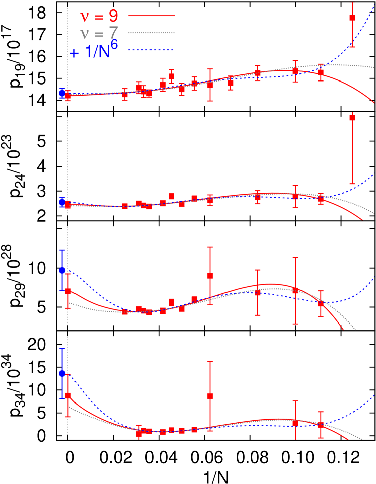
In Fig. 5 we compare the NSPT finite volume data with different fit functions for a few representative cases. We plot our primary fit function Eq. (42) with $\nu=9$ and with $\nu=7$, and the fit function including the $1/N^{6}$-effect Eq. (43) with $\nu=8$. We also show our final results for the infinite volume coefficients $p_{n}$ (last column of Table 4), as well as the results from the fit including the $1/N^{6}$-effects (first column of Table 4). From these figures the change of the curvature of the fit function due to the running of $\alpha((Na)^{-1})$, that becomes more pronounced as we increase the order $n$, is apparent. The increase in curvature is expected from the asymptotic renormalon analysis, see Sec. V below. We remark that the differences between our larger lattices, i.e. $40\geq N\geq 24$, and the values extrapolated to $N=\infty$ are much smaller here than they were in the case of the Polyakov line Bali:2013pla where we went up to $N(=N_{S})=16$.

Table 5: Ratios $p_{n}/(np_{n-1})$ for different values of $\nu$ using the fit function Eq. (42), in analogy to Table 3. The expectations from diagrammatic perturbation theory are $p_{1}/p_{0}=1.278414323(14)$ and $p_{2}/(2p_{1})=2.53952(9)$.

$\nu$	$13$	$11$	$9$	$7$
$p_{1}/p_{0}$	$1.27867(16)$	$1.278506(60)$	$1.278464(31)$	$1.278434(28)$
$p_{2}/(2p_{1})$	$2.53869(36)$	$2.53929(17)$	$2.53936(11)$	$2.539406(95)$
$p_{3}/(3p_{2})$	$2.21811(22)$	$2.21794(15)$	$2.21799(11)$	$2.21803(10)$
$p_{4}/(4p_{3})$	$1.91087(34)$	$1.91088(21)$	$1.91085(14)$	$1.91088(12)$
$p_{5}/(5p_{4})$	$1.66528(81)$	$1.66549(62)$	$1.66542(38)$	$1.66540(20)$
$p_{6}/(6p_{5})$	$1.4708(11)$	$1.47078(98)$	$1.47125(69)$	$1.47110(29)$
$p_{7}/(7p_{6})$	$1.3150(12)$	$1.3150(10)$	$1.31514(75)$	$1.31547(35)$
$p_{8}/(8p_{7})$	$1.18831(96)$	$1.18824(86)$	$1.18811(64)$	$1.18865(35)$
$p_{9}/(9p_{8})$	$1.08374(74)$	$1.08367(69)$	$1.08404(52)$	$1.08406(42)$
$p_{10}/(10p_{9})$	$0.99555(90)$	$0.99559(82)$	$0.99583(65)$	$0.99624(59)$
$p_{11}/(11p_{10})$	$0.9204(15)$	$0.9205(14)$	$0.9209(11)$	$0.92142(87)$
$p_{12}/(12p_{11})$	$0.8555(26)$	$0.8556(21)$	$0.8558(17)$	$0.8554(14)$
$p_{13}/(13p_{12})$	$0.7996(34)$	$0.7993(27)$	$0.7998(22)$	$0.8002(19)$
$p_{14}/(14p_{13})$	$0.7505(41)$	$0.7499(33)$	$0.7507(26)$	$0.7510(23)$
$p_{15}/(15p_{14})$	$0.7069(49)$	$0.7065(40)$	$0.7071(31)$	$0.7074(28)$
$p_{16}/(16p_{15})$	$0.6679(60)$	$0.6680(50)$	$0.6682(37)$	$0.6684(33)$
$p_{17}/(17p_{16})$	$0.6330(73)$	$0.6331(62)$	$0.6339(44)$	$0.6339(40)$
$p_{18}/(18p_{17})$	$0.6015(86)$	$0.6020(74)$	$0.6028(52)$	$0.6029(47)$
$p_{19}/(19p_{18})$	$0.573(10)$	$0.5758(88)$	$0.5742(61)$	$0.5743(54)$
$p_{20}/(20p_{19})$	$0.548(13)$	$0.549(10)$	$0.5495(70)$	$0.5495(62)$
$p_{21}/(21p_{20})$	$0.526(15)$	$0.528(11)$	$0.5263(78)$	$0.5260(70)$
$p_{22}/(22p_{21})$	$0.504(17)$	$0.510(13)$	$0.5063(87)$	$0.5049(79)$
$p_{23}/(23p_{22})$	$0.485(19)$	$0.495(14)$	$0.4883(97)$	$0.4847(90)$
$p_{24}/(24p_{23})$	$0.470(21)$	$0.482(16)$	$0.473(11)$	$0.467(11)$
$p_{25}/(25p_{24})$	$0.463(25)$	$0.475(20)$	$0.461(14)$	$0.452(13)$
$p_{26}/(26p_{25})$	$0.462(28)$	$0.473(27)$	$0.453(17)$	$0.440(16)$
$p_{27}/(27p_{26})$	$0.462(33)$	$0.478(38)$	$0.450(22)$	$0.430(20)$
$p_{28}/(28p_{27})$	$0.468(39)$	$0.489(49)$	$0.456(28)$	$0.429(26)$
$p_{29}/(29p_{28})$	$0.485(49)$	$0.505(59)$	$0.471(34)$	$0.438(32)$
$p_{30}/(30p_{29})$	$0.523(61)$	$0.537(61)$	$0.492(39)$	$0.459(38)$
$p_{31}/(31p_{30})$	$0.512(63)$	$0.527(60)$	$0.509(37)$	$0.489(37)$
$p_{32}/(32p_{31})$	$0.513(62)$	$0.528(57)$	$0.522(34)$	$0.517(33)$
$p_{33}/(33p_{32})$	$0.503(65)$	$0.519(57)$	$0.527(31)$	$0.535(31)$
$p_{34}/(34p_{33})$	$0.518(56)$	$0.530(46)$	$0.540(24)$	$0.566(26)$

Table 6: Ratios $p_{n}/(np_{n-1})$ for different fits. For details see the caption of Table 4. In the last column we display the final values including their statistical and systematic errors.

	$1/N^{6}$	$\beta_{3}\neq 0$	$\beta_{2}=0$	${\rm Final\;result}$
$p_{1}/p_{0}$	$1.278554(54)$	$1.278464(31)$	$1.278464(31)$	$1.278464(43)$
$p_{2}/(2p_{1})$	$2.53916(17)$	$2.53936(11)$	$2.53936(11)$	$2.53936(12)$
$p_{3}/(3p_{2})$	$2.21793(15)$	$2.21799(11)$	$2.21799(11)$	$2.21799(12)$
$p_{4}/(4p_{3})$	$1.91081(22)$	$1.91086(14)$	$1.91086(14)$	$1.91085(15)$
$p_{5}/(5p_{4})$	$1.66504(67)$	$1.66512(18)$	$1.66542(39)$	$1.66542(38)$
$p_{6}/(6p_{5})$	$1.47077(99)$	$1.47174(48)$	$1.47123(69)$	$1.47125(70)$
$p_{7}/(7p_{6})$	$1.3151(10)$	$1.31515(73)$	$1.31515(76)$	$1.31514(82)$
$p_{8}/(8p_{7})$	$1.18827(81)$	$1.18802(63)$	$1.18812(64)$	$1.18811(83)$
$p_{9}/(9p_{8})$	$1.08368(58)$	$1.08391(46)$	$1.08404(52)$	$1.08404(52)$
$p_{10}/(10p_{9})$	$0.99541(74)$	$0.99568(62)$	$0.99582(65)$	$0.99583(77)$
$p_{11}/(11p_{10})$	$0.9205(13)$	$0.9214(12)$	$0.9209(11)$	$0.9209(12)$
$p_{12}/(12p_{11})$	$0.8560(19)$	$0.8561(17)$	$0.8558(17)$	$0.8558(17)$
$p_{13}/(13p_{12})$	$0.8000(25)$	$0.7997(22)$	$0.7998(22)$	$0.7998(22)$
$p_{14}/(14p_{13})$	$0.7510(30)$	$0.7508(26)$	$0.7507(26)$	$0.7507(26)$
$p_{15}/(15p_{14})$	$0.7077(36)$	$0.7069(31)$	$0.7071(31)$	$0.7071(31)$
$p_{16}/(16p_{15})$	$0.6692(43)$	$0.6683(37)$	$0.6682(37)$	$0.6682(37)$
$p_{17}/(17p_{16})$	$0.6346(51)$	$0.6343(44)$	$0.6338(44)$	$0.6339(44)$
$p_{18}/(18p_{17})$	$0.6039(61)$	$0.6029(52)$	$0.6027(52)$	$0.6028(52)$
$p_{19}/(19p_{18})$	$0.5761(72)$	$0.5743(61)$	$0.5742(61)$	$0.5742(61)$
$p_{20}/(20p_{19})$	$0.5509(85)$	$0.5494(70)$	$0.5495(70)$	$0.5495(70)$
$p_{21}/(21p_{20})$	$0.5277(98)$	$0.5257(79)$	$0.5264(78)$	$0.5263(78)$
$p_{22}/(22p_{21})$	$0.508(11)$	$0.5056(87)$	$0.5064(87)$	$0.5063(88)$
$p_{23}/(23p_{22})$	$0.492(14)$	$0.4876(96)$	$0.4883(97)$	$0.488(10)$
$p_{24}/(24p_{23})$	$0.480(16)$	$0.471(11)$	$0.473(11)$	$0.473(12)$
$p_{25}/(25p_{24})$	$0.474(20)$	$0.459(13)$	$0.461(14)$	$0.461(16)$
$p_{26}/(26p_{25})$	$0.473(24)$	$0.449(15)$	$0.453(17)$	$0.453(22)$
$p_{27}/(27p_{26})$	$0.478(28)$	$0.445(19)$	$0.451(22)$	$0.450(30)$
$p_{28}/(28p_{27})$	$0.490(32)$	$0.449(24)$	$0.457(29)$	$0.456(39)$
$p_{29}/(29p_{28})$	$0.510(33)$	$0.463(29)$	$0.472(34)$	$0.471(47)$
$p_{30}/(30p_{29})$	$0.537(33)$	$0.484(34)$	$0.494(39)$	$0.492(51)$
$p_{31}/(31p_{30})$	$0.536(29)$	$0.502(33)$	$0.511(37)$	$0.509(42)$
$p_{32}/(32p_{31})$	$0.531(25)$	$0.515(29)$	$0.524(34)$	$0.522(34)$
$p_{33}/(33p_{32})$	$0.522(25)$	$0.521(28)$	$0.529(31)$	$0.527(32)$
$p_{34}/(34p_{33})$	$0.523(22)$	$0.537(23)$	$0.542(24)$	$0.540(35)$

We now determine the infinite volume $p_{n}/(np_{n-1})$-ratios. These can be obtained from the same fits, since we have also computed the correlation matrices. The results for different values of $\nu$ using our default fit function are displayed in Table 5. We find strong correlations between the errors of consecutive expansion coefficients. Due to these correlations, the infinite volume $p_{n}/(np_{n-1})$-ratios are more precise than the coefficients themselves. We compute the central values and the errors of the ratios in the same way as we did for the coefficients. We show the results for the different variations of the fit function we discussed above in Table 6. Again in the last column we display our final numbers. For the coefficients $p_{n}$ the statistical and systematic errors were of similar magnitudes. In the case of the ratios the total errors are dominated by statistics. The systematics cancel to a large extent and also the relative statistical uncertainties are somewhat reduced, due to the above-mentioned correlations between subsequent orders.

Whereas we could determine the coefficients $p_{n}$ and their ratios with reasonable accuracy, this is not the case for the $1/N^{4}$ correction coefficients $f_{n}$ and $c_{n}$: these become compatible with zero within errors (albeit with central values significantly bigger than the $p_{n}$). However, these parameters need to be included and their correlations are important to achieve acceptable fit qualities.

V Asymptotic behaviour of the expansion coefficients

In this section we confront the infinite volume coefficients $p_{n}$ obtained in Sec. IV with their large-$n$ dependence expected from the renormalon picture. We start by presenting our theoretical expectations. Then we compare these against the numerical data, extract the normalization of the leading renormalon and compare this with other determinations. We conclude estimating the intrinsic ambiguity of truncated perturbative series.

V.1 Renormalon analysis of the plaquette

The renormalon-associated large-$n$ dependence of the coefficients $p_{n}$ means the perturbative expansion of the plaquette is asymptotically divergent and its summation ambiguous. This ambiguity is not arbitrary but such that it can be absorbed by higher dimensional terms of the OPE, in our case by the gluon condensate $\langle O_{\mathrm{G}}\rangle$ (of dimension $d=4$) times its Wilson coefficient $C_{\mathrm{G}}$ (see Eq. (32)). This fixes the large-$n$ dependence of the $p_{n}$. Successive contributions to the sum $p_{n}\alpha^{n+1}$ should decrease for increasing orders $n$ down to a minimum contribution for $n_{0}\sim 1/(a_{d}\beta_{0})$, where $a_{d}=\beta_{0}/(2\pi d)$ (for a more detailed discussion see Sec. V.4 below). After this order the series starts to diverge. Assuming the ambiguity of the sum to be of the order of the minimum term we have $p_{n_{0}}\alpha^{n_{0}+1}\sim\exp[-1/(a_{d}\alpha)]\sim\Lambda_{\mathrm{QCD}}^{d}a^{d}$, which can be absorbed redefining the gluon condensate.

For notational convenience we introduce the following parametrization of the integrated inverse $\beta$-function:

$$\Lambda=\mu\exp\left\{-\left[\frac{2\pi}{\beta_{0}\alpha(\mu)}+b\ln\left(\frac{1}{2}\frac{\beta_{0}\alpha(\mu)}{2\pi}\right)+\sum_{j\geq 1}s_{j}\,(-b)^{j}\!\left(\frac{\beta_{0}\alpha(\mu)}{2\pi}\right)^{\!j}\right]\right\}$$ (44)

with

$$b=\frac{\beta_{1}}{2\beta_{0}^{2}}\,,\quad s_{1}=\frac{\beta_{1}^{2}-\beta_{0}\beta_{2}}{4b\beta_{0}^{4}}\,,\quad s_{2}=\frac{\beta_{1}^{3}-2\beta_{0}\beta_{1}\beta_{2}+\beta_{0}^{2}\beta_{3}}{16b^{2}\beta_{0}^{6}}\,.$$ (45)

Note that the expansion coefficients $c_{k}$ defined in Eq. (27) are related to the above constants for the case of the Wilson action:

$$c_{0}=-b\frac{\beta_{0}}{2\pi}\,,\quad c_{1}=s_{1}b\left(\frac{\beta_{0}}{2\pi}\right)^{\!2}\,,\quad c_{2}=-2s_{2}b^{2}\left(\frac{\beta_{0}}{2\pi}\right)^{\!3}\,.$$ (46)

The best way to quantify the asymptotic behaviour of the perturbative series is by performing its Borel transform:

$$B[P_{\mathrm{pert}}]\equiv\sum_{n=0}^{\infty}\frac{p_{n}}{n!}\left(\frac{4\pi}{\beta_{0}}u\right)^{\!n}\,.$$ (47)

The Borel transform of the expansion of the plaquette will have a singularity, due to the dimension four gluon condensate, at $u=d/2=2$:

$$B[P_{\mathrm{pert}}]=N_{P}\,\frac{1}{(1-2u/d)^{1+db}}\left[1+b_{1}\left(1-\frac{2u}{d}\right)+b_{2}\,\frac{db}{db-1}\left(1-\frac{2u}{d}\right)^{2}+\cdots\right]\,,$$ (48)

where (the second equalities apply to the Wilson action case)

$$b_{1} =ds_{1}+\frac{2\pi c_{0}}{\beta_{0}b}=ds_{1}-1\,,$$ (49)

$$b_{2} =\frac{4\pi^{2}c_{1}}{\beta_{0}^{2}b^{2}}+ds_{1}\left(\frac{ds_{1}}{2}+\frac{2\pi c_{0}}{\beta_{0}b}\right)-ds_{2}=ds_{1}\left(\frac{ds_{1}}{2}-1+\frac{1}{db}\right)-ds_{2}\,.$$ (50)

We skip the detailed derivation, which is quite standard (see, e.g., Ref. Beneke:1998ui ), and directly state the result of the Borel integral for large orders $n$:

$$p_{n} \stackrel{{\scriptstyle n\rightarrow\infty}}{{=}}N_{P}\,\left(\frac{\beta_{0}}{2\pi d}\right)^{\!n}\frac{\Gamma(n+1+db)}{\Gamma(1+db)}\left\{1+\frac{db}{n+db}\,b_{1}\right.$$ (51)

$$\qquad\left.+\frac{(db)^{2}}{(n+db)(n+db-1)}\,b_{2}+\mathcal{O}\left(\frac{1}{n^{3}}\right)\right\}\,.$$

Note that the parameters $b_{1}$ and $b_{2}$ that describe the leading pre-asymptotic corrections depend on the expansion coefficients $c_{0}$ and $c_{1}$, defined in Eq. (27), of the Wilson coefficient of the gluon condensate.

In the lattice scheme the numerical values read

$$p^{\mathrm{latt}}_{n} \stackrel{{\scriptstyle n\rightarrow\infty}}{{=}}N^{\mathrm{latt}}_{P}\,\left(\frac{\beta_{0}}{2\pi d}\right)^{\!n}\frac{\Gamma(n+1+db)}{\Gamma(1+db)}$$ (52)

$$\qquad\times\left\{1+\frac{20.08931\ldots}{n+db}+\frac{505\pm 33}{\left(n+db\right)\left(n+db-1\right)}+\mathcal{O}\left(\frac{1}{n^{3}}\right)\right\}\,.$$

We observe that the pre-asymptotic corrections are quite large, suggesting that high orders $n>20$ are required to reach the asymptotic regime. Regarding this, it is illustrative to show the corresponding expansion in the $\overline{\mathrm{MS}}$ scheme:

$$p^{\overline{\mathrm{MS}}}_{n} \stackrel{{\scriptstyle n\rightarrow\infty}}{{=}}N^{\overline{\mathrm{MS}}}_{P}\,\left(\frac{\beta_{0}}{2\pi d}\right)^{\!n}\frac{\Gamma(n+1+db)}{\Gamma(1+db)}$$ (53)

$$\qquad\times\left\{1-\frac{3.13653\ldots}{n+db}-\frac{1.1005\ldots}{\left(n+db\right)\left(n+db-1\right)}+\mathcal{O}\left(\frac{1}{n^{3}}\right)\right\}\,.$$

In this case the $1/n$ corrections are much smaller, suggesting the asymptotic regime to be reached at much lower orders in the $\overline{\mathrm{MS}}$ scheme (as was seen in Ref. Bali:2013pla for the expansion of the energy of a static source).

Note that $N_{P}$ dictates the strength of the renormalon behaviour of any quantity where the first non-perturbative effect is proportional to the gluon condensate. Only the pre-asymptotic effects will depend on the observable in question, due to different Wilson coefficients. This motivates us to define

$$N_{\mathrm{G}}=\frac{36}{\pi^{2}}N_{P}\,,$$ (54)

which is normalized in the same way as the gluon condensate.

$\langle P\rangle$ is a well-defined observable: it can be unambiguously computed in non-perturbative lattice simulations. Only after performing its OPE, renormalon ambiguities show up. They appear within individual terms of the OPE expansion but have to cancel in the complete sum. Eq. (51) incorporates the leading renormalon behaviour of $P_{\mathrm{pert}}$, associated to the dimension four ($u=2$) matrix element. Dimension six ($u=3$) and higher order matrix elements in the OPE will result in additional subleading renormalon contributions to $P_{\mathrm{pert}}$. These, however, are exponentially suppressed in $n$, relative to the leading renormalon, and can be neglected.

More delicate, and of higher practical relevance, is the possible renormalon cancellation between dimension four and six matrix elements. This corresponds to a renormalon of dimension $6-4=2$ and implies that $C_{\mathrm{G}}(\alpha)$ may have a renormalon itself to achieve this cancellation. From the Borel plane point of view, we would then have

$$B[C_{\mathrm{G}}]\sim\frac{1}{1-u}\,.$$ (55)

Since the plaquette $a^{-4}P$ is a trivial multiple of the Wilson gauge action Lagrange density, it can be related to the trace anomaly:

$$a^{4}T^{\mathrm{latt}}_{\mu\mu}=\frac{9\beta(\alpha)}{\pi\alpha^{2}}P\,.$$ (56)

This equality can be used to define the $\beta$-function in the lattice scheme and this in turn allowed us to relate the Wilson coefficient of the gluon condensate $C_{\mathrm{G}}$ to the $\beta$-function in Eq. (27). Since each $c_{k}$-coefficient contains a term proportional to $\beta^{\mathrm{latt}}_{k+1}$, the perturbative $\beta$-function will have a dimension two infrared ambiguity, corresponding to a renormalon at $u=1$. This can also be seen directly starting from the expectation value of the trace of the energy-momentum tensor Eq. (26): with the Wilson gauge action this equals $\langle T_{\mu\mu}^{\mathrm{latt}}\rangle$ up to $a^{2}\langle O_{6}\rangle$-type corrections. Defining the $\beta$-function through the trace anomaly Eq. (26) then results in the high-order behaviour of the coefficients $\beta_{i}$ to be determined by a dimension two renormalon. Note that this does not imply that expansions of observables in terms of $\alpha(a^{-1})$ are affected by this singularity. However, running $\alpha$ to a different scale will result in a $u=1$ divergent behaviour. This should not come as a surprise since also in non-perturbative lattice simulations masses etc. are subject to $\mathcal{O}(a^{2}\Lambda_{\mathrm{QCD}}^{2})$ corrections under changes of the lattice scale $a$. Note that the above arguments are specific for the plaquette and the lattice scheme. We would not expect the $\overline{\mathrm{MS}}$ scheme $\beta$-function to receive renormalon contributions.

We could be worried about the existence of ultraviolet renormalons in the perturbative expansion of the plaquette, which we have neglected in the above discussion. However, we do not see any indication of alternating signs in the expansion of the plaquette. Theoretically, this absence of ultraviolet renormalons is expected since these can only appear when integrating over momenta much bigger than the scale of $\alpha$. In our case this scale is $1/a$, which is close to the maximum possible momentum $\sqrt{4}\pi/a$ that can be realized on a four dimensional lattice: due to the hard cut-off perturbative expansions are ultraviolet finite.

Renormalons are not the only possible sources of divergences. However, other singularities, e.g., due to tunnelling instabilities are further removed from the origin of the Borel plane. For instance, instanton contributions are suppressed by factors $\sim\exp(-2\pi/\alpha)$ for the case of TBC on symmetric lattices 'tHooft:1981sz ; vanBaal:1982ag and, therefore, can only appear at $u\geq\beta_{0}/2\gg 2$.

Finally, for the ratios Eq. (51) implies

$$\frac{p_{n}}{np_{n-1}} =\frac{\beta_{0}}{2\pi d}\left\{1+\frac{db}{n}+\frac{db(1-ds_{1})}{n^{2}}\right.$$ (57)

$$\qquad+\left.\frac{db\left[1-3ds_{1}+d^{2}b(s_{1}+2s_{2})\right]}{n^{3}}+\mathcal{O}\left(\frac{1}{n^{4}}\right)\right\}\,.$$

The $1/n^{2}$- and $1/n^{3}$-correction terms depend on the coefficients $c_{0}$ and $c_{1}$, which we eliminated from the above equation via Eq. (46) (see also Eqs. (49) and (50)). We remark that Eq. (57) is a prediction, without any free parameters, since $N_{P}$ cancels from the ratio.

V.2 Comparison to the numerical data

The infinite volume extrapolation of the $p_{n}(N)$ made in Sec. IV only used the OPE structure of the finite size effects. No assumption was made about the divergent behaviour of the perturbative series. We now compare the extrapolated $p_{n}$-data with the renormalon-based expectations at large orders $n$. We also determine the normalization of the leading renormalon of the plaquette $N_{P}$ (and the associated one of the gluon condensate $N_{\mathrm{G}}=(36/\pi^{2})N_{P}$) and convert this into the $\overline{\mathrm{MS}}$ scheme.

Figure 6: The ratios $p_{n}/(np_{n-1})$ compared with the prediction Eq. (57) for the LO, next-to-leading order (NLO), NNLO and NNNLO of the $1/n$-expansion. Only the “$N=\infty$” extrapolation includes the systematic uncertainties. We also show finite volume data for $N=28$, and the result from the alternative $N\rightarrow\infty$ extrapolation including $1/N^{6}$ corrections. The symbols have been shifted slightly horizontally.

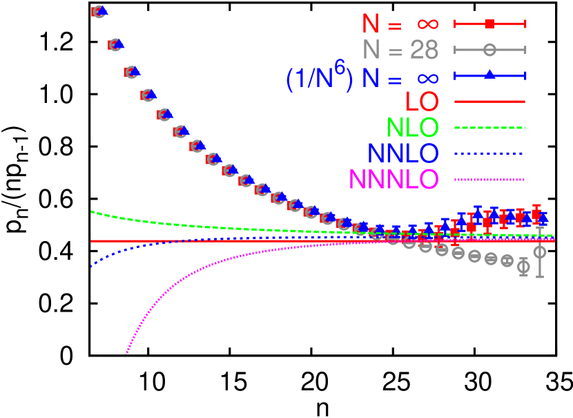
In Fig. 6 we compare our infinite volume $p_{n}/(np_{n-1})$-ratios, summarized in the last column of Table 6, to Eq. (57), truncating at different orders in the $1/n$-expansion. As expected from the numerical values displayed in Eq. (52), we see quite substantial differences between the leading order (LO), next-to-leading order (NLO), NNLO and NNNLO curves. Therefore, in our Wilson lattice scheme, we can only hope to detect the asymptotic behaviour for orders $n\gtrsim 20$. Indeed, the data are in agreement with the expectations for orders $n\geq 24$. For the highest three orders ($n\geq 32$) the data are somewhat above the expectation. However, these points are highly correlated and at the very limit of what was achievable for us, so we will not over-interpret this behaviour.

In conclusion, the $p_{n}/(np_{n-1})$-ratios for $n\gtrsim 24$ clearly indicate the existence of a renormalon at $u=2$. The coefficients $p_{n}$ are certainly diverging and their asymptotic behaviour is clearly inconsistent with other parametrizations, e.g., a singularity at $u=1$. Unfortunately, we do not have enough precision to quantitatively investigate subleading $1/n$-effects.

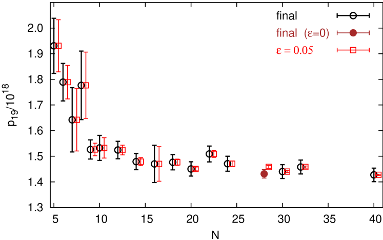
Next, we investigate the behaviour of the finite size effects. We expect the expansion coefficients of $\langle O_{\mathrm{G}}\rangle_{\mathrm{soft}}$, i.e. the $f_{n}$ of Eq. (15), to be governed by a dimension four ($u=2$) renormalon due to its mixing with the Wilson coefficient of the unity operator, i.e. $P_{\mathrm{pert}}$. On a lattice with a fixed finite extent $N$ the divergence of the $f_{n}$ will, at very high orders, result in an exponentiation of the associated logarithms, effectively cancelling the $1/N^{4}$ suppression and the divergence of the $p_{n}$. This will then, in the absence of non-perturbative terms, result in a convergent expansion of $\langle P\rangle_{\mathrm{pert}}(N)$. Therefore, finite size effects are expected to become big for $n\gtrsim 24$. To illustrate this, we also display the finite volume $N=28$ data in Fig. 6. Indeed, for $n\gtrsim 24$, differences between the $N=28$ data and the $N=\infty$ extrapolation become visible. This is discussed in detail in Ref. Bali:2013pla for the case of the expansion of the static energy. In Eq. (76) of this reference $\beta_{0}$ needs to be replaced by $\beta_{0}/d$, effectively quadrupling the order $n$ where this effect becomes relevant, and $e^{\ln N_{S}}/N_{S}$ replaced by $e^{4\ln N}/N^{4}$ accordingly. This behaviour also results in a more pronounced curvature of the fit function at large $N$-values due to the running of $\alpha((Na)^{-1})$, as we increase the order $n$ (see Fig. 5). Nevertheless, for the plaquette, these running effects get obscured by the $u=1$ renormalon of the Wilson coefficient $C_{\mathrm{G}}$, since the $c_{k}$ saturate towards the asymptotic behaviour at lower orders than the $f_{n}$ and then diverge more rapidly ($c_{k}\sim k\beta_{0}/(4\pi)c_{k-1}$ rather than $f_{n}\sim n\beta_{0}/(8\pi)f_{n-1}$). However, in this asymptotic regime the $1/N^{6}$ coefficients $g_{n}$ are also expected to diverge, the associated logarithms to exponentiate and to cancel against the $c_{k}/N^{4}$- and $p_{n}$-contributions.

Our fits are consistent with the above picture. We expect that our primary fit, which does not incorporate $\mathcal{O}(1/N^{6})$ terms, only provides an effective parametrization of $1/N^{4}$ and $1/N^{6}$ renormalon-associated effects. We first observe that setting the Wilson coefficient $C_{\mathrm{G}}$ to one, i.e. $c_{k}=0$, we cannot simultaneously account for the $u=2$ renormalon of the $f_{n}$ parameters and for the effects of the $u=1$ renormalon on the $c_{k}$ parameters. Within our primary fit we observe the central values of the parameters $f_{n}$ and $c_{k}$ to grow much faster towards high orders than the $p_{n}$-coefficients. This is consistent with the existence of a $u=1$ renormalon since, in the absence of $1/N^{6}$-terms, cancellations have to take place between combinations of $f_{n}$- and $c_{k}$-terms. In any case, we remark that the individual coefficients all carry large relative errors of $\mathcal{O}(1)$. Therefore, these statements are qualitative in nature rather than quantitative. A reliable determination of the $c_{k}$- and $f_{n}$-coefficients (and of their expected divergences) requires a full $\mathcal{O}(1/N^{6})$ analysis, with six additional fit parameters per order of the expansion, which is beyond our reach. Instead, we partially included the leading $\mathcal{O}(1/N^{6})$ logarithms into our fits according to Eq. (43). As a result, the growth of the $c_{k}$-coefficients becomes more consistent with a $u=1$ renormalon. Also the $g_{n}$-values are observed to grow much faster towards high orders than the $p_{n}$-coefficients. The coefficients $f_{n}$ are comparatively smaller in size than the $c_{n}$ and $g_{n}$ but larger than the corresponding $p_{n}$. Also in this case, all the finite size coefficients carry large relative errors of $\mathcal{O}(1)$, making this discussion, at most, qualitative.

Fortunately, for the coefficients $p_{n}$ the $1/N^{6}$-effects are only subleading and, as can be read off from Table 4, their values change very little when adding some of these higher order effects. The errors of our infinite volume coefficients $p_{n}$ in the last column of Table 4 already incorporate these systematics. We illustrate this by including the extrapolation to infinite $N$, incorporating a $1/N^{6}$-term (first column of Table 6), into Fig. 6. The errors displayed in this case are only statistical.

It is worth mentioning that in the case of the static energy studied in Refs. Bauer:2011ws ; Bali:2013pla ; Bali:2013qla the Wilson coefficient of the leading (in this case $d=1$) finite volume correction was exactly one. Consequently, there were no ambiguities that had to be absorbed by even higher dimensional operators. Therefore, the above complication was not encountered and we were not only able to reliably determine the infinite volume expansion coefficients but also the coefficients of the $1/N$ finite volume correction term.

V.3 Determination of $N_{P}$

Figure 7: $N_{P}$, determined from the coefficients $p_{n}$ via Eq. (51) truncated at NLO, NNLO and NNNLO. The green box marks our final result quoted in Eq. (58). The data are slightly adjusted horizontally.

To obtain the normalization $N_{P}$ we divide the coefficients displayed in Table 4 by Eq. (51) truncated at different orders in $1/(n+db)$, labelled as (for consistency with Eq. (57) and Fig. 6) NLO, NNLO and NNNLO, respectively. For large $n$-values these ratios should tend to constants, allowing us to extract $N_{P}$. This is depicted in Fig. 7. We observe the three data sets are compatible with constant values for $n\gtrsim 24$. In Fig. 7 we also observe that truncating Eq. (51) at different orders in $1/(n+db)$ produces large corrections. Fortunately enough, however, they follow a convergent pattern, with smaller differences between the NNLO and NNNLO curves than between the NLO and NNLO curves. We also note that in the range $25\leq n\leq 30$, where we regard the prediction as most reliable, the inclusion of higher order $1/n$ effects results in a flatter dependence on $n$.

We take the value of the NNNLO evaluation for $n=26$, where it exhibits a very mild maximum, as our central value. For $n<25$ we may not have reached the asymptotic behaviour whereas for $n>30$ the results become less meaningful, due to the exploding errors. The uncertainty of the determination of $N_{P}$ is dominated by the pre-asymptotic effects, which are large in the lattice scheme. We use the difference between the NNNLO and NNLO determinations at $n=26$ as an estimate for even higher order effects and add this in quadrature to the (comparatively small) error of the NNNLO prediction:

$$N_{P}^{\mathrm{latt}}=42(17)\times 10^{4}\,, \qquad N^{\mathrm{latt}}_{\mathrm{G}}=1.54(63)\times 10^{6}\,,$$

$$N_{P}^{\overline{\mathrm{MS}}}=0.61(25)\,, \qquad N^{\overline{\mathrm{MS}}}_{\mathrm{G}}=2.24(92)\,.$$ (58)

For the last two equalities we have used the exact identity

$$N^{\overline{\mathrm{MS}}}_{P}=N^{\mathrm{latt}}_{P}\Lambda^{4}_{\mathrm{latt}}/\Lambda^{4}_{\overline{\mathrm{MS}}}\,,$$ (59)

where Hasenfratz:1980kn ; Luscher:1995np $\Lambda_{\overline{\mathrm{MS}}}\approx 28.809338139488\,\Lambda_{\mathrm{latt}}$. Note that the normalization of the plaquette renormalon in the $\overline{\mathrm{MS}}$ scheme is of $\mathcal{O}(1)$, as it is the case for the renormalon of the heavy quark pole mass [cf. Eq. (105) of Ref. Bali:2013pla , or Eq. (11) of Ref. Bali:2013qla ].

We have also explored alternative methods to determine $N_{P}$. One is using the relation

$$N_{P}=\left.B[P_{\mathrm{pert}}](u)(1-2u/d)^{1+bd}\right|_{u=2}$$ (60)

to compute $N_{P}$ as a perturbative expansion in $u$ Lee:1996yk . However, this did not work, which may not be surprising since the singularity is located at $u=2$, very far away from the origin. One may also consider a conformal mapping to move the singularity closer to the origin. Again, we do not obtain the expected plateau behaviour for the orders of the expansion that we have at our disposal. This is consistent with the analysis made in Ref. Bali:2013pla , where this method became compatible with the asymptotic expectation only at much higher orders (compare Fig. 12 with Fig. 14 of this reference) than the method we outlined and employed above. In Ref. Bali:2013pla we were able to go to orders $(n+1)/d\leq 20$ rather than $(n+1)/d\leq 35/4$ and ultimately found agreement between the two determinations.

We now compare Eq. (58) with previous estimates available in the literature. The large-$\beta_{0}$ result can be found, for instance, in Refs. Broadhurst:1992si ; Beneke:1998ui :

$$N^{\overline{\mathrm{MS}}}_{P,\mathrm{large-\beta_{0}}}=\frac{e^{10/3}}{24\pi}\approx 0.37178\,.$$ (61)

This is 40% smaller than our central value but within errors still consistent with our result $N_{P}^{\overline{\mathrm{MS}}}=0.61(25)$. There also exist estimates from the perturbative expansion of the Adler function. In Ref. Beneke:2008ad the first four orders were used to fit the expected leading renormalon singularities in the Borel plane (see also the discussion in Ref. Beneke:2012vb ). The result was $N^{\overline{\mathrm{MS}}}_{P}\approx 0.02$ for $n_{f}=3$. For the case of $n_{f}=0$, which corresponds to our setting, this model yields Matthias $N^{\overline{\mathrm{MS}}}_{P}\approx 0.04$ (note the strong dependence on $n_{f}$). In Ref. Lee:2011te the value 0.01 was obtained using the conformally mapped version of Eq. (60) for the Adler function. We remark that using the method of Ref. Lee:2011te we were not able to obtain the renormalon normalization with our $\mathcal{O}(\alpha^{35})$ perturbative expansion. While these numbers differ quite substantially from each other, all of them are significantly smaller than our determination. We believe that the main difficulty with these analyses is that the perturbative expansion of the Adler function is not known to sufficiently high orders to probe the $u=2$ renormalon. Also in our case, see Fig. 7, lower orders would have given smaller numbers. While it should not be necessary to go up to $n>20$ to detect the renormalon in the $\overline{\mathrm{MS}}$ scheme, also in this case orders four times higher than for the heavy quark pole mass renormalon at $u=1/2$ probably are necessary.

V.4 Partial sum and minimal term

In the regime where the coefficients $p_{n}$ are dominated by the renormalon behaviour, we can determine the order $n_{0}$ that corresponds to the minimal term of the perturbative series from the analytical expectation Eq. (51). Minimizing $p_{n}\alpha^{n+1}$ results in

$$(n_{0}+db)\frac{\beta_{0}\alpha}{2\pi d}=\exp\left\{-\frac{1}{2(n_{0}+db)}+\mathcal{O}\left[\frac{1}{(n_{0}+db)^{2}}\right]\right\}\,.$$ (62)

This then gives the minimal term

$$p_{n_{0}}\alpha^{n_{0}+1} =\frac{2\pi d^{1/2+db}}{2^{db}\Gamma{(1+db)}}\sqrt{\frac{\alpha}{\beta_{0}}}N_{P}\exp\!\left(-\frac{2\pi d}{\beta_{0}\alpha}\right)\left(\frac{\beta_{0}\alpha}{4\pi}\right)^{-db}\left[1+\mathcal{O}(\alpha)\right]$$ (63)

$$\approx\frac{2\pi d^{1/2+db}}{2^{db}\Gamma{(1+db)}}\sqrt{\frac{\alpha}{\beta_{0}}}(\Lambda a)^{4}\,.$$

While the perturbative series is divergent, truncating it at the order ${n_{\mathrm{max}}}\simeq n_{0}(\alpha)$,

$$S_{P}(\alpha)=\sum_{n=0}^{n_{\max}}p_{n}\alpha^{n+1}\,,$$ (64)

results in a finite sum (this is equivalent to a particular scheme to subtract the renormalon).

By taking ${n_{\mathrm{max}}}\simeq n_{0}$ we minimize the dependence of the series on the order at which it is truncated. We assign the uncertainty of the sum due to the truncation to be

$$\delta S_{P}=\sqrt{n_{0}}\,p_{n_{0}}\alpha^{n_{0}+1}\approx\frac{(2\pi)^{3/2}d^{1+db}}{2^{db}\beta_{0}\,\Gamma{(1+db)}}N_{P}(\Lambda a)^{4}\approx 12.06\,N_{P}(\Lambda a)^{4}\,.$$ (65)

This object is scheme- and scale-independent (to the $1/n$-precision that we employed in the above derivation) because, even though the normalization $N_{P}$ depends on the scheme, the product $N_{P}\Lambda^{4}$ is scheme-independent. A higher order calculation should yield an expression that is proportional to the product of Eq. (65) and the Wilson coefficient $C_{\mathrm{G}}$, since the ambiguity of the truncated sum must cancel against a similar ambiguity of the contribution from the gluon condensate.

Figure 8: The combination $\sqrt{n}\,p_{n}\alpha^{n+1}/(\Lambda_{\mathrm{latt}}a)^{4}$, see Eq. (66), as a function of $n$ for $\beta=5.3,5.8,6.3,6.8$ and 7.3. The error band corresponds to the theoretical expectation $12.06\,N_{P}=5.1(2.1)\times 10^{6}$ of Eq. (65), where we have used the value of Eq. (58) for $N_{P}$. The data sets have been adjusted horizontally for better legibility. Note that the left-most points correspond to $n=1$.

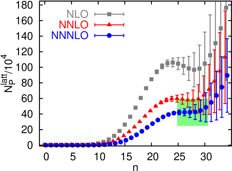
In Fig. 8 we plot the combination

$$\frac{\sqrt{n}\,p_{n}\alpha^{n+1}}{(\Lambda a)^{4}}\approx\sqrt{n}\,p_{n}\alpha^{n+1}\displaystyle{e^{4\left[\frac{2\pi}{\beta_{0}\alpha}+b\ln\left(\frac{1}{2}\frac{\beta_{0}\alpha}{2\pi}\right)-s_{1}b\frac{\beta_{0}\alpha}{2\pi}+s_{2}b^{2}\left(\frac{\beta_{0}\alpha}{2\pi}\right)^{\!2}\right]}}$$ (66)

as a function of $n$ where we substitute $1/(\Lambda a)^{4}$ by the integrated four-loop $\beta$-function of Eq. (44). For $n\simeq n_{0}$

$$\left.\frac{\sqrt{n}\,p_{n}\alpha^{n+1}}{(\Lambda a)^{4}}\right|_{n=n_{0}}=\frac{\delta S_{P}}{(\Lambda a)^{4}}\simeq 12.06\,N_{P}\,,$$ (67)

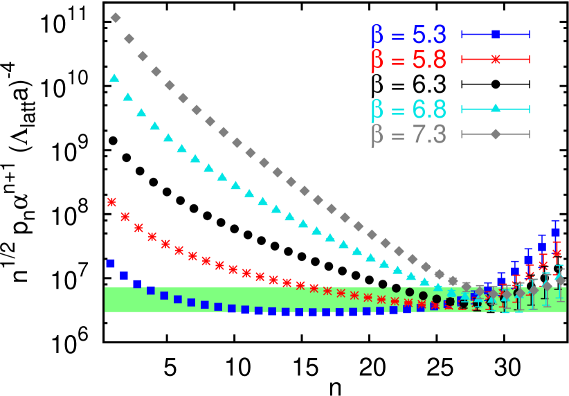
so it should approach the value $12.06\,N_{P}=5.1(2.1)\times 10^{6}$ [Eq. (65) with the $N_{P}$-value of Eq. (58)], drawn as an error band. The comparison is made for $\beta=3/(2\pi\alpha)=5.3,5.8,6.3,6.8$ and $7.3$. The three values $\beta=5.8,6.3$ and 6.8 are typical for present-day non-perturbative lattice simulations, with inverse lattice spacings $1.4\,\mathrm{GeV}\lesssim a^{-1}\lesssim 6.4\,\mathrm{GeV}$ Necco:2001xg , while $\beta=5.3$ is in the strong-coupling regime.

The corresponding $n_{0}$-predictions Eq. (62) are, in ascending order of the $\beta$-values $n_{0}\simeq 24,26,28,30$ and 33. In the figure we have multiplied the minimal term by $\sqrt{n}$ which then corresponds to the uncertainty of the truncated series. Note that the variation of $\sqrt{n}$ for $24\leq n\leq 33$ can be neglected on the logarithmic scale of the figure. As expected, the contributions to the sum decrease monotonously down to the minimum at orders that, within errors and for $\beta\geq 5.8$, are consistent with the above expectations on $n_{0}$. Thereafter, the contributions start to diverge. The ambiguity computed from the data agrees perfectly with the prediction. This is quite remarkable, as the sizes of the different terms of the perturbative series cover several orders of magnitude.

The effect of truncating the integrated $\beta$-function Eq. (44) at different orders in Eq. (66) is sizeable because $|\beta_{2}^{\mathrm{latt}}|$ and $|\beta_{3}^{\mathrm{latt}}|$ are numerically large and $d=4$. The $1/(n+db)$- and $1/(n+db)^{2}$-terms of Eq. (51) (for numerical values see Eq. (52)) have the same origin. Including the $s_{1}\alpha$- or $s_{2}\alpha^{2}$-terms into Eq. (66) has a similar effect as the inclusion of the $1/n$- or $1/n^{2}$-terms had on the determination of the normalization $N_{P}$, see Fig. 7. Therefore, best agreement is achieved truncating Eq. (66) at the order in $\alpha$ associated to the respective $1/n$ truncation of the $N_{P}$-determination. The Wilson coefficient $C_{\mathrm{G}}$ that we have ignored so far would reduce the data points by only a few per cent within the range of couplings covered by the figure and can safely be neglected.

It is interesting to see that the order at which the series starts exploding can be delayed by decreasing the coupling, i.e. going to larger $\beta$-values, however, the ambiguity of the expansion remains the same since its origin lies in the inherent ambiguity of the definition of the non-perturbative gluon condensate. We estimate this ambiguity using the result Eq. (58) for $N_{\mathrm{G}}^{\overline{\mathrm{MS}}}$, the prefactor of Eq. (65) and the value Capitani:1998mq ; Necco:2001xg $\Lambda_{\overline{\mathrm{MS}}}(n_{f}=0)=0.602(48)r_{0}^{-1}\approx 238~{}\mathrm{MeV}$:

$$\delta\langle O_{\mathrm{G}}\rangle_{\mathrm{NP}}\simeq\left.\frac{(2\pi)^{3/2}d^{1+db}}{2^{db}\beta_{0}\,\Gamma{(1+db)}}\,N_{\mathrm{G}}^{\overline{\mathrm{MS}}}\right|_{n_{f}=0}\Lambda_{\overline{\mathrm{MS}}}^{4}=27(11)\,\Lambda_{\overline{\mathrm{MS}}}^{4}\sim 0.087\,\mathrm{GeV}^{4}\,.$$ (68)

$n_{f}=0$ relates to the $n_{f}$-dependence of $\beta_{0}$ and $b$. The above value is bigger than standard estimates of the non-perturbative gluon condensate Vainshtein:1978wd $\sim 0.012\,\mathrm{GeV}^{4}$, and indicates that determinations of this quantity may significantly depend on the way the perturbative series is truncated or approximated. Note that the large-$\beta_{0}$ limit of Eq. (68) (using Eq. (61)) yields a considerably smaller number, which, however, is still bigger than standard estimates:

$$\delta\langle O_{\mathrm{G}}\rangle_{\mathrm{NP},\mathrm{large-\beta_{0}}}\simeq\left.\frac{(2\pi)^{3/2}}{\beta_{0}}\,\frac{6e^{10/3}}{\pi^{3}}\right|_{n_{f}=0}\Lambda_{\overline{\mathrm{MS}}}^{4}\simeq 7.77\,\Lambda_{\overline{\mathrm{MS}}}^{4}\sim 0.025\,\mathrm{GeV}^{4}\,.$$ (69)

Eqs. (68) and (69) have been computed for $n_{f}=0$. The prefactors multiplying $N_{\mathrm{G}}^{\overline{\mathrm{MS}}}$ only show a mild $n_{f}$-dependence in both cases. While the large-$\beta_{0}$ limit of $N_{\mathrm{G}}^{\overline{\mathrm{MS}}}$ is $n_{f}$ independent, beyond this approximation the $n_{f}$-dependence of $N_{\mathrm{G}}^{\overline{\mathrm{MS}}}$ is unknown.

VI Summary and Conclusions

The expectation value of the (infinite volume) plaquette can be expanded as follows

$$\langle P\rangle=P_{\mathrm{pert}}(\alpha)\langle\mathds{1}\rangle+a^{4}\frac{\pi^{2}}{36}C_{\mathrm{G}}(\alpha)\langle O_{\mathrm{G}}\rangle_{\mathrm{NP}}+\mathcal{O}(a^{6})\,,$$ (70)

where $\langle O_{\mathrm{G}}\rangle_{\mathrm{NP}}$ is the renormalization group invariant definition of the non-perturbative gluon condensate and $C_{\mathrm{G}}(\alpha)=1+\mathcal{O}(\alpha)$ is its Wilson coefficient. In our numerical stochastic perturbation theory simulation, we calculated the coefficients $p_{n}(N)$ of the perturbative expansion

$$\langle P\rangle_{\mathrm{pert}}(N)=\sum_{n\geq 0}p_{n}(N)\alpha^{n+1}\,$$ (71)

in lattice regularization with the Wilson gauge action up to $\mathcal{O}(\alpha^{35})$ on lattices of up to $40^{4}$ points, using twisted boundary conditions (TBC) in three directions. The choice of TBC turned out to be superior to periodic boundary conditions, not only in terms of statistical errors and reduced finite volume effects, but also because only these boundary conditions allow for a systematic analysis of finite volume effects in the framework of the operator product expansion (OPE). This enabled us to accurately obtain the infinite volume extrapolation of the $p_{n}$-coefficients:

$$P_{\mathrm{pert}}=\lim_{N\rightarrow\infty}\langle P\rangle_{\mathrm{pert}}(N)\qquad{\rm and}\qquad p_{n}=\lim_{N\rightarrow\infty}p_{n}(N)\,,$$ (72)

as well as of their ratios $p_{n}/(np_{n-1})$. The results are summarized in the last columns of Tables 4 and 6. We have analysed their high-order behaviour and found the $p_{n}$-coefficients to diverge from orders $n\gtrsim 24$ onwards in a way consistent with a renormalon at $u=2$ in the Borel plane, as expected from the dimensionality $d=4$ of the gluon condensate. This is illustrated in Fig. 6. We stress that we were only able to obtain this result after having achieved both good theoretical control of finite volume effects and computing the perturbative expansion to orders as high as $\alpha^{35}$.

Furthermore, we have determined the normalization $N_{P}$ of the corresponding renormalon (see Eqs. (48) and (51) for its definition):

$$N_{P}^{\mathrm{latt}}=42(17)\times 10^{4}\,.$$ (73)

This can be converted from the lattice into the $\overline{\mathrm{MS}}$ scheme at arbitrary precision since the combination $N_{P}\Lambda^{4}$ is scheme-independent. We obtained $N_{P}^{\overline{\mathrm{MS}}}=0.61(25)$ in the $\overline{\mathrm{MS}}$ scheme, which differs by 2.5 standard deviations from zero. Still, a 40% error on $N_{P}\Lambda^{4}$ translates into a 10% error on the $d=1$ combination $N_{P}^{1/4}\Lambda$. Alternatively, we can normalize the series accompanying $\langle\mathds{1}\rangle$ consistently with respect to $\langle O_{\mathrm{G}}\rangle$, to obtain the normalization of the renormalon associated to the gluon condensate:

$$N^{\overline{\mathrm{MS}}}_{\mathrm{G}}=\frac{36}{\pi^{2}}N_{P}^{\overline{\mathrm{MS}}}=2.24\pm 0.92\,.$$ (74)

This is independent of any pre-asymptotic effects and therefore of the observable in question. From this value we can also estimate the intrinsic truncation ambiguity of corresponding perturbative expansions, see Eqs. (65) and (68),

$$\delta\langle O_{\mathrm{G}}\rangle_{\mathrm{NP}}\simeq(27\pm 11)\,\Lambda_{\overline{\mathrm{MS}}}^{4}\,.$$ (75)

This is larger than standard estimates of the non-perturbative gluon condensate Vainshtein:1978wd $\sim 0.012$. Therefore, determinations of this quantity may significantly depend on the way the perturbative series is truncated or approximated. The above value is by a factor of 3.5 bigger than the large-$\beta_{0}$ result and by about one order of magnitude larger than many previous estimates of the ambiguity of the gluon condensate, see, for instance, Eq. (5.12) of Ref. Beneke:1998ui . This is mainly due to the large prefactor relating $N_{P}$ to $\delta S_{P}$ in Eq. (65), and $N_{\mathrm{G}}$ to $\delta\langle O_{\mathrm{G}}\rangle_{\mathrm{NP}}$ in Eq. (68). Finally, we remark that we obtain a similar uncertainty just by computing $\sqrt{n_{0}}p_{n_{0}}\alpha^{n_{0}+1}$ directly from the data, see Fig. 8, thereby verifying this large prefactor.

The magnitude of pre-asymptotic $1/n$- and $1/n^{2}$-corrections was the main limiting factor for the precision of Eq. (74). In our case, we suffered from large coefficients $|\beta_{2}^{\mathrm{latt}}|$ and $|\beta_{3}^{\mathrm{latt}}|$. This is not the case in the $\overline{\mathrm{MS}}$ scheme. Actually, there are strong indications (see, e.g., Ref. Pineda:2001zq ) that renormalon dominance for the pole mass in the $\overline{\mathrm{MS}}$ scheme sets in already at orders as low as $n\lesssim 2$. Therefore, in this scheme perturbative expansions of observables with non-perturbative contributions from $\langle O_{\mathrm{G}}\rangle_{\mathrm{NP}}$ may show the expected asymptotic behaviour already for orders $n\lesssim 8\ll 24$. However, a direct translation of the perturbative coefficients from the lattice to the $\overline{\mathrm{MS}}$ scheme is not possible, since the necessary conversion is not known to such high orders. In Ref. Bali:2013pla we experimented with resumming the expansion by re-defining the coupling, without changing the action or observable, so that it resembled a $\overline{\mathrm{MS}}$-like scheme. This resulted in an earlier on-set of the asymptotic behaviour, however, at the price of much larger statistical errors so that the determination of the normalization could not be improved upon. Alternatively, it is conceivable that other lattice discretizations with smaller $\Lambda_{\overline{\mathrm{MS}}}/\Lambda_{\mathrm{latt}}$-ratios will have smaller high-order $\beta$-function coefficients, resulting in renormalon dominance at smaller orders $n$. In particular, the $\mathcal{O}(a^{2})$ Symanzik-improved action Weisz:1982zw ; Luscher:1984xn would be worthwhile to study. Unfortunately, in this case fewer analytic and semi-analytic low-order results are available. Finally, we would also like to stress that pre-asymptotic effects do not only depend on the $\beta$-function coefficients but also on $C_{\mathrm{G}}$. Therefore, the on-set of renormalon dominance depends both on the renormalization scheme and on the observable in question.

Our analysis may immediately impact on phenomenological analyses in cases where the perturbative series is sensitive to the gluon condensate renormalon. Even though one should bear in mind that we have only studied the pure gauge $n_{f}=0$ theory, it is worth mentioning that for the pole mass renormalon ($u=1/2$) the $n_{f}$ dependence has been found to be mild. In that case an analysis analogous to the one performed in the present paper yielded a precision of 6% for the associated normalization $N_{m}\Lambda$ Bali:2013qla for the $n_{f}=0$ theory. The resulting value was only 8% off of the $n_{f}=3$ result obtained in Ref. Pineda:2001zq from the pole mass perturbative expansion (up to orders $n=3$) in the $\overline{\mathrm{MS}}$ scheme. It is also reassuring that the $n_{f}$-dependence of the large-$\beta_{0}$ result is under control (with a difference of $\sim 20$% between the $n_{f}=3$ and $n_{f}=0$ results of Eq. (69)). In any case, it would certainly be worthwhile to repeat our investigation using a different gauge action and incorporating fermions. Such future studies will not change, however, the qualitative picture or the main conclusions presented here.