Measuring mass-loss rates and constraining shock physics using X-ray line profiles of O stars from the Chandra archive

Abstract

We quantitatively investigate the extent of wind absorption signatures in the X-ray grating spectra of all non-magnetic, effectively single O stars in the Chandra archive via line profile fitting. Under the usual assumption of a spherically symmetric wind with embedded shocks, we confirm previous claims that some objects show little or no wind absorption. However, many other objects do show asymmetric and blue shifted line profiles, indicative of wind absorption. For these stars, we are able to derive wind mass-loss rates from the ensemble of line profiles, and find values lower by an average factor of 3 than those predicted by current theoretical models, and consistent with ${\rm H}{\alpha}$ if clumping factors of $f_{\rm cl}\approx 20$ are assumed. The same profile fitting indicates an onset radius of X-rays typically at $r\approx 1.5$ ${R_{\ast}}$, and terminal velocities for the X-ray emitting wind component that are consistent with that of the bulk wind. We explore the likelihood that the stars in the sample that do not show significant wind absorption signatures in their line profiles have at least some X-ray emission that arises from colliding wind shocks with a close binary companion. The one clear exception is $\zeta$ Oph, a weak-wind star that appears to simply have a very low mass-loss rate. We also reanalyse the results from the canonical O supergiant $\zeta$ Pup, using a solar-metallicity wind opacity model and find $\dot{M}=1.8\times 10^{-6}$ ${\mathrm{M_{\sun}~{}{\mathrm{y}r^{-1}}}}$, consistent with recent multi-wavelength determinations.

1 Introduction

By losing mass at a rate of $\dot{M}\sim 10^{-6}$ ${\mathrm{M_{\sun}~{}{\mathrm{y}r^{-1}}}}$ via its stellar wind, an O star can shed a significant portion of its mass over the course of its lifetime (Puls et al., 2008). Not only can this substantially reduce the mass of a core-collapse supernova progenitor, but the wind transfers a significant amount of mass, momentum, and energy to the surrounding interstellar medium (ISM). Thus, the wind mass-loss rate is an important parameter in the study of both stellar evolution and of the Galactic environment. In recent years there has been increased awareness of large systematic uncertainties in many mass-loss rate diagnostics, primarily due to wind clumping, rendering the actual mass-loss rates of O stars somewhat controversial (e.g. Fullerton et al. 2006; Oskinova et al. 2007; Sundqvist et al. 2010).

X-rays provide a potentially good clumping-insensitive mass-loss rate diagnostic via the effect of wind attenuation on X-ray emission line profile shapes. The characteristic line profile shape that provides the diagnostic power arises because redshifted photons emitted from the rear hemisphere of the wind are subject to more attenuation than the blueshifted photons originating in the front hemisphere (MacFarlane et al. 1991; Owocki & Cohen 2001; see fig. 2 of Cohen et al. 2010a). The degree of blue shift and asymmetry in these line profiles is then directly proportional to the wind column density and thus to the mass-loss rate. By fitting a simple quantitative model (Owocki & Cohen, 2001) to each emission line in a star’s spectrum and then analysing the ensemble of line optical depths, we can determine the star’s mass-loss rate (Cohen et al., 2010a, 2011). Complementary approaches that fit all the lines simultaneously, along with fitting the broadband X-ray properties, have also been employed recently (Hervé et al., 2012, 2013). While our approach does not use as many different observational constraints it does have the advantage of simplicity, which enables us to more easily explore the effects of individual line properties, particularly those involving hot plasma kinematics and absorption by the cold wind component, which are the focus of this paper.

Because this X-ray absorption line profile diagnostic scales with the column density rather than the square of the density, it avoids many of the problems presented by traditional mass-loss rate diagnostics. In particular, UV resonance line diagnostics are problematic due to their sensitivity to ionization corrections which are highly uncertain and are sensitive to clumping effects on density-squared recombination (Bouret et al., 2005). Further complications arise with UV lines from optically thick clumping, including velocity-space clumping (Oskinova et al., 2007; Owocki, 2008; Sundqvist et al., 2010, 2011). For direct density-squared diagnostics such as ${\rm H}{\alpha}$ and radio or IR free-free emission, the mass-loss rate will be overestimated if clumping is not accounted for. And even when clumping is accounted for, there is a degeneracy between the mass-loss rate and the clumping factor, as the quantity derived from these diagnostics is $\dot{M}\sqrt{{f_{\mathrm{c}l}}}$ where the clumping factor, $f_{\rm cl}\equiv\langle\rho^{2}\rangle/\langle\rho\rangle^{2}$. Using the X-ray absorption diagnostic in conjunction with the density-squared emission diagnostics can break this degeneracy and enable us to simultaneously determine the mass-loss rate and the clumping factor.

Recent, more sophisticated application of the density-squared emission diagnostics (${\rm H}{\alpha}$, IR and radio free-free), assuming a radially dependent clumping factor, has led to a downward revision of empirical mass-loss rates of O stars (Puls et al., 2006). These lowered mass-loss rates provide a natural explanation for the initially surprising discovery (Cassinelli et al., 2001; Kahn et al., 2001) that X-ray line profiles are not as asymmetric as traditional mass-loss rate estimates had implied.

Table 1: Properties of programme stars

Star	Spectral Type	$T_{\rm eff}$	$R$	log $g$	$v_{\infty}$	MEG counts	HEG counts	exposure time
		(kK)	($\mathrm{R_{\sun}}$)	(cm s-2)	(km s-1)			(ksec)
HD 93129A	O3 If*	42.5a	22.5a	3.71a	3200a	2936	1258	137.7
HD 93250	O3.5 V	46.0a	15.9a	3.95a	3250b	6169	2663	193.7
9 Sgr	O4 V	42.9c	12.4c	3.92c	3100b	4530	1365	145.8
$\zeta$ Pup	O4 If	40.0d	18.9d	3.63d	2250b	11018	2496	73.4
HD 150136	O5 III	40.3c	15.1c	3.69c	3400b	8581	2889	90.3
Cyg OB2 8A	O5.5 I	38.2e	25.6e	3.56e	2650e	6575	1892	65.1
HD 206267	O6.5 V	37.9c	9.61c	3.92c	2900b	1516	419	73.5
15 Mon	O7 V	37.5f	9.9f	3.84f	2150b	1621	393	99.8
$\xi$ Per	O7.5 III	35.0a	14.0a	3.50a	2450b	5603	1544	158.8
$\tau$ CMa	O9 II	31.6c	17.6c	3.41c	2200b	1300	311	87.1
$\iota$ Ori	O9 III	31.4f	17.9f	3.50f	2350b	4836	1028	49.9
$\zeta$ Oph	O9 V	32.0a	8.9a	3.65a	1550b	5911	1630	83.8
$\delta$ Ori	O9.5 II	30.6c	17.7c	3.38c	2100b	6144	1071	49.1
$\zeta$ Ori	O9.7 Ib	30.5c	22.1c	3.19c	1850b	9140	2003	59.6
$\epsilon$ Ori	B0 Ia	27.5g	32.4g	3.13g	1600b	6813	1474	91.7

References: ^aRepolust et al. (2004); ^bHaser (1995); ^cMartins et al. (2005); ^dNajarro et al. (2011); ^eMokiem et al. (2005); ^fMarkova et al. (2004); ^gSearle et al. (2008)

While small-scale, optically thin clumping can reconcile the X-ray, ${\rm H}{\alpha}$, IR, and radio data for these stars, there is no direct evidence for optically thick clumping, or porosity, in the X-ray data themselves (Cohen et al., 2008; Sundqvist et al., 2012; Hervé et al., 2013; Leutenegger et al., 2013). Porosity results from optically thick clumps, which can hide opacity in their interiors, enhancing photon escape through the interclump channels. While porosity has been proposed as an explanation for the more-symmetric-than-expected observed X-ray line profiles (Oskinova et al., 2006), very large porosity lengths are required in order for porosity to have any effect on line profiles (Owocki & Cohen, 2006; Sundqvist et al., 2012), and levels of porosity consistent with measured line profiles produce only modest (not more than about 25 per cent) effects on derived mass-loss rates (Leutenegger et al., 2013). In this paper, we derive mass-loss rates from the measured X-ray line profiles under the assumption that porosity extreme enough to significantly affect mass-loss rate determinations is not present.

The initial application of the X-ray line profile based mass-loss rate diagnostic to the O supergiant $\zeta$ Pup gave a mass-loss rate of $\dot{M}=3.5\times 10^{-6}$ ${\mathrm{M_{\sun}~{}{\mathrm{y}r^{-1}}}}$ (Cohen et al., 2010a). This represents a factor of three reduction over the unclumped ${\rm H}{\alpha}$ value (Repolust et al., 2004; Puls et al., 2006), and is consistent with the newer analysis of ${\rm H}{\alpha}$, IR, and radio data which sets an upper limit of $\dot{M}<4.2\times 10^{-6}$ ${\mathrm{M_{\sun}~{}{\mathrm{y}r^{-1}}}}$ when the effects of clumping are accounted for (Puls et al., 2006). A similar reduction is found for the very early O supergiant, HD 93129A, where the X-ray mass-loss rate of $\dot{M}=6.8\times 10^{-6}$ ${\mathrm{M_{\sun}~{}{\mathrm{y}r^{-1}}}}$ is about a factor of 3.5 lower than inferred from unclumped ${\rm H}{\alpha}$ models, consistent with a clumping factor $f_{\rm cl}=3.5^{2}\approx 12$ (Cohen et al., 2011).

The goal of this paper is to extend the X-ray line profile mass-loss rate analysis to all the non-magnetic, effectively single O stars with grating spectra in the Chandra archive. It is already known that some, especially later-type, O stars show no obvious wind attenuation signatures (Miller et al., 2002; Skinner et al., 2008; Nazé et al., 2010; Huenemoerder et al., 2012), and as one looks towards weaker winds in early B (V - III) stars, the X-ray lines are not as broad as the wind velocities would suggest they should be (Cohen et al., 2008). Therefore, we have excluded from our sample very late-O main sequence stars with relatively narrow lines, but we do include late-O giants and supergiants, even when the profiles appear unaffected by attenuation. In these cases we want to quantify the level of attenuation that may be hidden in the noise, placing upper limits on their mass-loss rates. Of course, it is possible that the model assumptions break down for some of the stars in the sample, not least of all if wind-wind interactions with a binary companion are responsible for some of the X-ray emission, in which case an intrinsically symmetric emission line profile may dilute whatever attenuation signal is present.

An additional goal of this paper is to constrain wind-shock models of X-ray production by extracting kinematic and spatial information about the shock-heated plasma from the line profiles. The profiles are Doppler broadened by the bulk motion of the hot plasma embedded in the highly supersonic wind. Our quantitative line profile model allows us to derive an onset radius of hot plasma and also, for the highest signal-to-noise lines, the terminal velocity of the X-ray emitting plasma. We will use these quantities to test the predictions of numerical simulations of wind-shock X-ray production.

The paper is organized as follows: In the next section we describe the data and our sample of O stars taken from the Chandra archive. In §3 we describe our data analysis and modeling methodology including the line profile model, the line profile fitting procedure, and the derivation of the mass-loss rate from an ensemble of line fits. In §4 we present our results, including mass-loss rate determinations for each star in our sample, and in §5 we discuss the results for each star in the sample and conclude with a discussion of the implications of the line profile fitting results.

2 The Programme Stars

2.1 Observations

All observations reported on in this paper were made with Chandra’s High Energy Transmission Grating Spectrometer (HETGS) (Canizares et al., 2005). The HETGS has two grating arrays: the Medium and High Energy Gratings (MEG and HEG). The MEG has a FWHM spectral resolution of 0.023 Å, while the HEG has a resolution of 0.012 Å, but lower sensitivity at the wavelengths of the lines we analyse in this paper. The dispersion of the grating arrays onto the Advanced CCD Imaging Spectrometer (ACIS) CCDs lead to bin sizes of 5 and 2.5 mÅ for the MEG and HEG spectra, respectively. We used the standard reduction procedure (ciao 3.3 to 4.3) for most of the spectra, but for Cyg OB 8A, which is in a crowded field, care had to be taken to properly centroid the zeroth order spectrum of the target star, which necessitated the use of a customized reduction procedure within ciao.

The observed spectra consist of a series of collisionally excited emission lines superimposed on a primarily bremsstrahlung continuum. The lines arise from high ionization states: most lines are from helium-like or hydrogen-like ions from abundant (even atomic number) elements O through Si, and the remainder come from iron L-shell transitions, primarily in Fe  xvii, but also from higher stages, especially for stars with hotter plasma temperature distributions. Chandra is sensitive in the wavelength range from 1.2 to 31 Å (0.4 to 10 keV). However, the shortest-wavelength line we are able to analyse in our sample stars is the Si  xiv line at 6.182 Å and the longest is the O  vii line at 21.804 Å. The spectra vary in quality – from 1611 to 13514 total first-order MEG $+$ HEG counts – and some suffer from significant interstellar attenuation at longer wavelengths. These two factors determine the number of lines we are able to fit in each star.

2.2 The sample

We selected every O and very early B star in the Chandra archive as of 2009 with a grating spectrum – see xatlas (Westbrook et al., 2008) – that shows obviously wind-broadened emission lines, aside from $\zeta$ Pup and HD 93129A, which we have already analysed (Cohen et al., 2010a, 2011). We eliminated from our sample those stars with known magnetic fields that are strong enough to provide significant wind confinement (Petit et al., 2013) (this includes $\theta^{1}$ Ori C and $\tau$ Sco) and we also excluded obvious binary colliding wind shock (CWS) X-ray sources (such as $\gamma^{2}$ Vel and $\eta$ Car) which are generally hard and variable. Some objects remaining in the sample are possible CWS X-ray sources. They are included because their spectra – including their line profiles – do not obviously appear to deviate from the expectations of the embedded wind shock (EWS) scenario, although we give special scrutiny to the fitting results for these stars in §5. It should be noted that colliding wind binary systems can show non-thermal radio emission without having significant CWS X-ray emission. We also exclude main sequence stars and giants with spectral type O9.5 and later, as these stars (including $\sigma$ Ori A and $\beta$ Cru) have X-ray lines too narrow to be understood in the context of standard embedded wind shocks. We ended up including one B star, the supergiant $\epsilon$ Ori (B0 Ia), which has wind properties very similar to O stars. The sample stars and their important parameters are listed in Table 1. We also include HD 93129A and $\zeta$ Pup in the table, despite not reporting on their line profile fits in this paper, because we rederive their mass-loss rates and discuss the results for those two early O supergiants in conjunction with the results for the newly analysed stars in §4.

3 Modeling and Data Analysis Methodology

3.1 X-ray emission line profile model

We use the model of X-ray emission and absorption introduced by Owocki & Cohen (2001). This model has the benefit of describing a general X-ray production scenario, making few assumptions about the details of the physical mechanism that leads to the production of shock-heated plasma in the wind. The model does assume that the cold, absorbing material in the wind and the hot, X-ray-emitting material both follow a $\beta$-velocity law of the form

$$v=v_{\infty}(1-{R_{\ast}}/r)^{\beta},$$ (1)

where $v_{\infty}$, the terminal velocity of the wind, usually has a value between 1500 and 3500 km s^-1. The $\beta$ parameter, derived from ${\rm H}{\alpha}$ and UV lines, typically has a value close to unity. The model also assumes that the filling factor of X-ray emitting plasma is zero below some onset radius, ${R_{\mathrm{o}}}$, and is constant above ${R_{\mathrm{o}}}$. Such emission-measure models with constant filling factor reproduce observed line profiles quite well (Kramer et al., 2003; Cohen et al., 2006). As recently discussed by Owocki et al. (2013) (see their fig. 3 and section 4), in analogous models that explicitly account for the expected radiative nature of embedded shocks in the relatively dense winds of O-type stars, such fitting of the observed profiles requires a shock heating rate that declines with radius, roughly as $1/r^{2}$. With this adjustment, the form of the emission integral becomes quite similar to that in the constant filling-factor model. To preserve continuity with previous analyses (Owocki & Cohen, 2001; Kramer et al., 2003; Cohen et al., 2006, 2010a, 2011), we retain the latter model here, deferring to future work examination of the (likely minor) effects of detailed differences from a model that accounts explicitly for radiative cooling.

Our implementation of the X-ray line profile model optionally includes the effects of porosity (Owocki & Cohen, 2006; Sundqvist et al., 2012) and of resonance scattering (Leutenegger et al., 2007) on the individual line profile shapes. We explore the effects of resonance scattering for a subset of stars in our sample, but because porosity has been shown to have a negligible effect on observed X-ray profiles and derived mass-loss rates (Hervé et al., 2013; Leutenegger et al., 2013), we do not include its effects in the profile modeling.

The adjustable free parameters of the profile model are generally just the normalization, which is the photon flux, $F_{\rm line}$, the parameter that describes the onset radius of X-ray production, ${R_{\mathrm{o}}}$, and a fiducial optical depth parameter, $\tau_{\ast}$, which we describe below. For a few high signal-to-noise lines, we allow $v_{\infty}$, the wind terminal velocity, to be a free parameter of the fit as well. Otherwise, we fix this parameter at the literature value listed for the star in Table 1. The parameter ${R_{\mathrm{o}}}$ controls the widths of the line via the assumed wind kinematics represented by equation (1). Small values of ${R_{\mathrm{o}}}$ correspond to more X-ray production close to the star where the wind has a small Doppler shift, while large values of ${R_{\mathrm{o}}}$ indicate that most of the X-rays come from high Doppler shift regions in the outer wind. Hydrodynamic models show shocks developing about half a stellar radius above the surface of the star – albeit with some variation based on treatments of the line force parameters and of the lower boundary conditions in numerical simulations (Feldmeier et al., 1997; Runacres & Owocki, 2002; Sundqvist & Owocki, 2013).

The optical depth of the wind affects the blue-shift and asymmetry of the line profile. The optical depth at a given location in the wind, and thus at a given wavelength, is given by

$$\tau(p,z)=\int^{\infty}_{z}\kappa(r^{\prime})\rho(r^{\prime}){\rm d}z^{\prime}=\frac{\dot{M}}{4{\pi}{R_{\ast}}v_{\infty}}\int^{\infty}_{z}\frac{\kappa(r^{\prime}){R_{\ast}}{\rm d}z^{\prime}}{r^{\prime 2}(1-{R_{\ast}}/r^{\prime})^{\beta}},$$ (2)

where $p,z$ are the usual cylindrical coordinates: the impact parameter, $p$, is the projected distance from the z-axis centred on the star and pointing toward the observer, and $r\equiv\sqrt{p^{2}+z^{2}}$.The second equality arises from substituting the $\beta$-velocity law into the general equation for the optical depth and employing the mass continuity equation. The profile is calculated from

$$L_{\lambda}\propto\int^{\infty}_{{R_{\mathrm{o}}}}{\eta}e^{-\tau}{\rm d}V,$$ (3)

where $\eta$ is the X-ray emissivity, $\tau$ is calculated using equation (2), and the volume integral is performed over the entire wind above $r={R_{\mathrm{o}}}$.

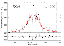
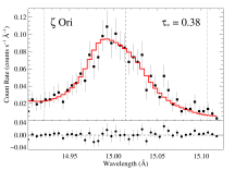
Figure 1: The Fe  xvii line at 15.014 Å with best-fitting model (top row) for three of the sample stars [$\zeta$ Oph, $\tau_{\ast}=0.00^{+.01}_{-.00}$ (left), $\xi$ Per, $\tau_{\ast}=0.22^{+.14}_{-.12}$ (middle), and $\zeta$ Ori, $\tau_{\ast}=0.38^{+.13}_{-.11}$ (right)] showing various degrees of asymmetry. The vertical dashed lines on the profile plots represent the laboratory line rest wavelength and the wavelengths corresponding to the terminal velocity of the wind. Note that the x-axis in each figure in the top row encompasses the same velocity range in units of the wind terminal velocity, but different absolute velocity and wavelength ranges, due to the different terminal velocities of the three stars’ winds. The star with the highest wind velocity, $\xi$ Per, is subject to more blending on its red wing than are the other two stars. The contours in the lower panels give the 68, 95, and 99.7 per cent two-dimensional joint confidence limits on $\tau_{\ast}$ and ${R_{\mathrm{o}}}$, while the best-fitting models are indicated by the filled circles.

We make an important, simplifying assumption at this point, which is that the continuum opacity, due to photoionization in the cold wind component, $\kappa(r)$, does not vary substantially with radius in the wind, and can be replaced with the spatially uniform average opacity, $\bar{\kappa}$, which we will henceforth write as $\kappa$ for simplicity. This enables us to pull the opacity out of the spatial optical depth integral in equation (2), leading to

$$\tau(p,z)=\tau_{\ast}\int^{\infty}_{z}\frac{{R_{\ast}}{\rm d}z^{\prime}}{r^{\prime 2}(1-{R_{\ast}}/r^{\prime})^{\beta}},$$ (4)

where the constant $\tau_{\ast}$, given by

$$\tau_{\ast}=\frac{\kappa\dot{M}}{4\pi{R_{\ast}}v_{\infty}},$$ (5)

is the single parameter that characterizes the effect of wind absorption on the line profile shape. And, along with the normalization, $F_{\rm line}$, and the ${R_{\mathrm{o}}}$ parameter described above, $\tau_{\ast}$ is the third free parameter of the profile model we fit to the data. We note that $\tau_{\ast}$ is an explicit analytic expression for the fiducial optical depth parameter, $\tau_{\rm o}$, first identified by MacFarlane et al. (1991) as the key parametrization of X-ray line profile shift and asymmetry in the shock-heated winds of OB stars.

It is key for using X-ray profile fitting to measure mass-loss rates that $\tau_{\ast}$ scales with $\dot{M}$, but it should be kept in mind that $\tau_{\ast}$ also is wavelength dependent, via its dependence on the opacity, $\kappa$. We hasten to point out, though, that while the continuum opacity varies from line to line, it does not vary significantly across a given line. We discuss the wind opacity, and especially its radial dependence and the effect of our taking it to be radially uniform, further in §3.3.

3.2 Fitting procedure

All model fitting was done in xspec (v12.3 to 12.6). We fit the positive and negative first order spectra simultaneously, but not co-added. Co-added spectra are shown in the figures for display purposes, however. When there were a significant number of counts in the HEG measurements of a given line, we included those data in the simultaneous fit. In most cases there were negligible counts in the HEG data and we fit only the MEG data. Because Poisson noise dominates these low-count Chandra data, we could not use $\chi^{2}$ as the fit statistic, and instead used the C statistic (Cash, 1979). As with $\chi^{2}$, a lower $C$ value indicates a better fit, given the same number of degrees of freedom. For placing confidence limits on model parameters, ${\Delta}C$ is equivalent to ${\Delta}\chi^{2}$ with a ${\Delta}C$ value of 1 corresponding to a 68 per cent confidence bound in one dimension (Press et al., 2007). We establish confidence bounds on the model parameters of interest one at a time, allowing other parameters to vary while establishing these bounds. There is generally a mild anti-correlation between ${R_{\mathrm{o}}}$ and $\tau_{\ast}$, so we also examined the joint constraints on two parameters, adjusting the corresponding value of ${\Delta}C$ accordingly. Joint confidence limits are shown in Fig. 1, along with the best-fitting models, for the Fe  xvii line at 15.014 Å for several stars with varying degrees of wind signature strength.

To account for the weak continuum under each emission line, we first fit a region around the line with a continuum model having a constant flux per unit wavelength. This continuum model was added to the line profile model when fitting the line itself. The fitting was generally then done with three free parameters: $\tau_{\ast}$, ${R_{\mathrm{o}}}$, and the normalization, $F_{\rm line}$. We fixed $\beta$ at 1, and $v_{\infty}$ at the value given in Table 1. A discussion of the effects of changing $\beta$ and $v_{\infty}$ as well as sensitivity to continuum placement, treatment of blends, and other aspects of our analysis can be found in Cohen et al. (2010a). For example, it is found that changing the wind velocity law exponent, $\beta$, from 1.0 to 0.8 generally leads to a change in the best-fitting $\tau_{\ast}$ and ${R_{\mathrm{o}}}$ values of between 10 and 20 per cent. One additional effect we account for is the radial velocity of each star. This effect was only significant for $\xi$ Per, which has $v_{r}=57$ km s^-1 (Hoogerwerf et al., 2001); no other star in the sample had a geocentric radial velocity during its Chandra observation that was this large.

Figure 2: Two different models for the wavelength-dependent opacity of the bulk wind, with the same simplified ionization balance assumed in each case, but altered C, N, and O abundances for the model shown as a dashed line. The solar abundance opacity model (solid) line is the one we use to derive mass-loss rates. Prominent ionization edges are labeled. Note the similarity of the two models shortward of the O K-shell edge, which is due to fact that despite the non-solar C, N, and O abundances, the metallicity, and thus the sum of the C, N, and O abundances, is solar for both models.

The hydrogen-like ${\rm Ly}{\alpha}$ lines in the spectra consist of two blended lines with wavelength separations that are much smaller than the resolution of the Chandra gratings. We fit these lines with a single model centred at the emissivity-weighted average of the two wavelengths. In some cases, the lines we wish to analyse are blended. If the blending is too severe to be modeled, as it is for the O  viii ${\rm Ly}{\beta}$ line at 16.006 Å, we excluded the line from our analysis entirely. If the blended portion of the line could be omitted from the fit range without producing unconstrained results, we simply fit the model over a restricted wavelength range. The Ne  x ${\rm Ly}{\alpha}$ line at 12.134 Å, for example, produces well-constrained results, even when its red wing is omitted due to blending with longer-wavelength iron lines. If lines from the same ion are blended, such as the Fe  xvii lines at 16.780, 17.051, and 17.096 Å, we fit three models to the data simultaneously, constraining the $\tau_{\ast}$ and ${R_{\mathrm{o}}}$ values to be the same for all the lines in the blended feature. In the case of the aforementioned iron complex, we also constrained the ratio of the normalizations of the two lines at 17.096 and 17.051 Å, which share a common lower level, to the theoretically predicted value (Mauche et al., 2001) because the blending is too severe to be constrained empirically.

The helium-like complexes are among the strongest lines in many of the sample stars’ spectra, but they are generally heavily blended. The forbidden-to-intercombination line intensity ratios are a function of the local mean intensity of the UV radiation at the location of the X-ray emitting plasma (Gabriel & Jordan, 1969; Blumenthal et al., 1972). And so the spatial (and thus velocity) distribution of the shock-heated plasma affects both the line intensity ratios and the line profile shapes. We model these effects in tandem and fit all three line profiles, including the relative line intensities, simultaneously, as described in Leutenegger et al. (2006). In order to do this, we use UV fluxes taken from tlusty (Lanz & Hubeny, 2003) model atmospheres appropriate for each star’s effective temperature and log $g$ values, as listed in Table 1. This procedure generates a single $\tau_{\ast}$ value and a single ${R_{\mathrm{o}}}$ value for the entire complex; where ${R_{\mathrm{o}}}$ affects both the line shapes and the $f/i$ ratios, as described above. We generally had to exclude the results for Ne  ix due to blending with numerous iron lines.

3.3 Analysing the ensemble of line fits from each star

To extract the mass-loss rate from a single derived $\tau_{\ast}$ parameter value, a model of the opacity of the cold, unshocked component of the wind is needed. Then, along with values for the wind terminal velocity and stellar radius, equation (5) can be used to derive a mass-loss rate for a given line by fitting the ensemble of $\tau_{\ast}(\lambda)$ values with $\dot{M}$ as the only free parameter. It has recently been shown for the high signal-to-noise spectrum of $\zeta$ Pup that if all lines in the spectrum are considered – but blends that cannot be modeled are excluded – and a realistic model of the wavelength-dependent wind opacity is used, then the wavelength trend in the ensemble of $\tau_{\ast}$ values is consistent with the atomic opacity (Cohen et al., 2010a). For other stars, the wavelength trend of $\tau_{\ast}$ expected from $\kappa(\lambda)$ may not be evident, but may still be consistent with it, as has been shown, recently, for HD 93129A (Cohen et al., 2011).

The opacity of the bulk, unshocked wind is due to bound-free absorption (inner shell photoionization), and the contributions from N, O, and Fe are dominant, with contributions from Ne and Mg at wavelengths below about 12 Å and some contribution from C and possibly He at long wavelengths, above the O K-shell edge near 20 Å (see Fig. 2; described in more detail below). Each element has non-zero bound-free cross section only at wavelengths shortwards of the threshold corresponding to the ionization potential. The cross-section is always largest at threshold and decreases roughly as $\lambda^{-3}$ below that. The combined contributions from each abundant element give the overall wind opacity a characteristic saw-tooth form, with overall opacity generally being higher at longer wavelengths, but also dependent on contributions from a smaller number of (low atomic number) elements at those long wavelengths. For a given element, higher ionization states have cross-section thresholds at modestly shorter wavelengths, but very similar cross-sections at all wavelengths below that. Thus, changes to the bulk wind ionization have only minor effects on the overall wind opacity.

The actual wind abundances – and uncertainties in and updates to their values – can affect the wind opacity, and thus the determination of a mass-loss rate from the ensemble of fitted $\tau_{\ast}$ values. However, as shown by Cohen et al. (2010a, 2011), the details of any non-solar abundances matter very little, although the overall opacity does scale as the metallicity and so derived mass-loss rates will be uncertain to the extent that overall metallicity is uncertain. However, future adjustments to metallicity determinations can be easily applied to the derived mass-loss rates, which we determine here assuming solar metallicity (Asplund et al., 2009). We make such a correction for $\zeta$ Pup below.

The main reason why the detailed abundances, and specifically CNO processing, matter very little is that the sum of the absolute abundances of these three elements should remain the same even if their relative concentrations are significantly altered. And at wavelengths below the O K-shell edge, all three elements contribute to the wind opacity and their cross-sections are very similar. Depleted O and enhanced N do in fact have an effect on the cross-section longward of the O K-shell edge where only N, C, and possibly He contribute to the wind opacity. So, enhanced nitrogen will increase the wind opacity longward of about 20 Å. However, partly because there are few strong lines in the Chandra bandpass at those long wavelengths and partly because the ISM is generally quite optically thick at long wavelengths, very few of our programme stars have any measured lines in the wavelength regime that would be affected by CNO processing and associated wind opacity modeling uncertainties.

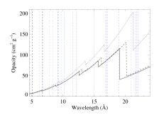
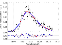
Figure 3: Left: Opacity models that demonstrate the greatest possible radial variation within a single, solar abundance, O star wind. Wavelengths of lines measured with the Chandra gratings are indicated by the vertical dashed (blue) lines, while the three different opacity models assume high ionization (metals in $+4$ and He fully ionized; solid), medium ionization (metals in $+3$ and He fully ionized; dashed) and low ionization (metals in $+2$ and He fully recombined to He  ii; dotted). Clearly, the metal ionization differences are a small effect, and the He recombination is the dominant effect, but is significant only longward of the oxygen K-shell edge near 20 Å. Middle: Opacities specific to $\zeta$ Pup, computed via detailed wind modeling using cmfgen, at three different radii in the wind (1.4, 3.9, 9.6 ${R_{\ast}}$ from solid to dashed, to dotted). (Note that the overall opacity, especially at long wavelengths, is somewhat higher than solar abundance models because of the helium abundance enhancement in $\zeta$ Pup and also somewhat higher than solar metallicity in the cmfgen model.) As expected, the opacity variation is small below the O K-shell edge, and larger above it, although not as large as the maximal scenario presented in the left panel. Right: A profile fit to the Fe  xvii line at 15.014 Å of $\zeta$ Pup (blue histogram) from a model where the wind opacity triples beyond $r\sim 5$ ${R_{\ast}}$ compared to a model with constant opacity (red histogram). The fit with the outer-wind opacity increase demonstrates a high degree of degeneracy with constant opacity models, but even in this extreme case, the decrease in $\tau_{\ast}$ is only 30 per cent, as can be seen by comparing the first and last rows of Table 2.

Table 2: Effect of outer wind opacity increase in $\zeta$ Pup

		Fe  xvii at 15.014 Å				O  viii at 18.969 Å
Extra opacity	$\tau_{\ast}$	Ro	C-stat		$\tau_{\ast}$	Ro	C-stat
0	1.92	1.56	280.79		2.99	1.22	150.89
0.5	1.78	1.58	282.17		2.82	1.24	150.68
1	1.66	1.60	283.45		2.66	1.26	150.68
2	1.48	1.62	285.71		2.31	1.34	150.98
3	1.33	1.63	287.66		1.86	1.53	151.22

Returning to ionization, the largest effect on the opacity due to differences or uncertainties in the ionization comes from recombination of He⁺⁺ to He⁺ in the outer wind. Fully ionized helium has no bound-free opacity but singly ionized helium has significant opacity at long wavelengths (the ionization edge is at ${\rm h}{\nu}=54.4$ eV; $\lambda=228$ Å), and can have an effect on the total wind opacity longward of the O K-shell edge near 20 Å. This, and other secondary ionization effects, can lead to some differences in the wind opacity as a function of radius (see, e.g., figs 1 and 2 of Hervé et al. 2013). However, the significant changes are almost entirely at the long-wavelength end of the Chandra bandpass, where helium has a disproportionate effect, and where there are very few, if any, emission lines in our programme stars’ spectra. Furthermore, although the opacity may change by roughly a factor of 2 in the outer wind, the density is so much lower there that the contribution of the outer wind to the column density – and thus the optical depth – along a typical sight line is negligible. For example, doubling the wind opacity beyond 5 ${R_{\ast}}$ increases the optical depth typically by only 10 per cent along sight-lines that pass through the densest parts of the wind.

Figure 4: The fitted $\tau_{\ast}$ values (points), along with the 68 per cent confidence limits (error bars), converted to a mass-loss rate, are shown for each line in each star. Lines for which the fitted $\tau_{\ast}$ values are within 1 $\sigma$ of zero are indicated as upper limits (at the best-fitting plus 1 $\sigma$ values). The fitted mass-loss rates for each star are indicated by the solid lines, while the dashed line in each panel represents the theoretical mass-loss rate listed in Table 3. Note that the y-axis range is the same in each panel, and that the best-fitting mass-loss rate for $\iota$ Ori is so low that it is off the bottom of that panel. For $\zeta$ Ori and $\epsilon$ Ori, we show the two and three points, respectively, omitted from the mass-loss rate fits because of resonance scattering (open squares).

Figure 5: The fitted ${R_{\mathrm{o}}}$ values for each line in each sample star (filled circles), along with the 68 per cent confidence limits (error bars). The best-fitting global ${R_{\mathrm{o}}}$ value for each star is indicated in each panel by the dashed line, while the dotted lines indicate the extent of the 68 per cent confidence limits. The excluded lines for $\zeta$ Ori and $\epsilon$ Ori are shown as open squares.

To further explore the uncertainty in the fitted $\tau_{\ast}$ values and ultimately the wind mass-loss rate, we tabulated three representative opacity models that span the widest possible ranges of ionization balance, and thus wind opacity. In Fig. 3 we show these models, and demonstrate that below the O K-shell edge, the wind can vary in opacity by only tens of per cent. And even above the edge the maximum variation is no more than a factor of 2. The key difference between the opacity models is the extent of helium recombination in the outer wind, which, at its most extreme, can double the opacity in the long-wavelength end of the Chandra bandpass. More modest opacity variations are seen in detailed models of the wind ionization computed with cmfgen (Hillier & Miller, 1998), also shown in Fig. 3. To test the effect of such a radial opacity increase on the derived $\tau_{\ast}$ values, we modified the line profile model to include a boost of the wind opacity above $r=5{R_{\ast}}$, and fit this model to two strong lines: Fe  xvii at 15.014 Å and O  viii at 18.969 Å. For each line we fit a sequence of models with different amounts of “extra” opacity in the far wind; with a radial profile given by $y=1-(1+(r/5{R_{\ast}})^{6})^{-0.5}$, where $y$ is the extra opacity, which can be scaled by any desired factor. The results of these experiments – the best-fitting $\tau_{\ast}$ and ${R_{\mathrm{o}}}$ and the value of the fit statistic for each value of $y$ that we tested – are reported in Table 2, where it can be seen, for example, that doubling the outer wind opacity decreases the line optical depth parameter, $\tau_{\ast}$, but only by about 15 per cent.

Table 3: X-ray derived results for each star

Star	Spectral type	$\dot{M}_{\rm theory}$	$\dot{M}$	$\chi^{2}$	${\rm N}_{lines}$	${R_{\mathrm{o}}}$	$\chi^{2}$	Primarily EWS?
		(${\mathrm{M_{\sun}~{}{\mathrm{y}r^{-1}}}}$)	(${\mathrm{M_{\sun}~{}{\mathrm{y}r^{-1}}}}$)			(${R_{\ast}}$)
HD 93129A	O2 If*	$1.2\times 10^{-5}$	$6.8^{+2.8}_{-2.4}\times 10^{-6}$	1.1	5	$1.34^{+.10}_{-.11}$	0.8	Yes
HD 93250	O3.5 V	$6.0\times 10^{-6}$	$1.2^{+1.5}_{-1.2}\times 10^{-7}$	0.3	3	$2.09^{+.15}_{-.13}$	2.6	No
9 Sgr	O4 V	$2.1\times 10^{-6}$	$3.7^{+1.0}_{-0.9}\times 10^{-7}$	3.3	7	$1.66^{+.05}_{-.05}$	5.8	Yes
$\zeta$ Pup	O4 If	$6.4\times 10^{-6}$	$1.76^{+0.13}_{-0.12}\times 10^{-6}$	10.6	16	$1.50^{+.03}_{-.03}$	13.6	Yes
HD 150136	O5 III	$2.3\times 10^{-6}$	$9.4^{+4.0}_{-4.1}\times 10^{-8}$	8.8	7	$1.35^{+.02}_{-.02}$	17.6	No
Cyg OB2 8A	O5.5 I	$8.7\times 10^{-6}$	$8.0^{+5.1}_{-5.1}\times 10^{-7}$	3.0	4	$1.54^{+.04}_{-.04}$	1.2	No
$\xi$ Per	O7.5 III	$9.3\times 10^{-7}$	$2.2^{+0.6}_{-0.5}\times 10^{-7}$	11.0	9	$1.57^{+.05}_{-.04}$	5.3	Yes
$\iota$ Ori	O9 III	$5.5\times 10^{-7}$	$3.2^{+84.}_{-3.2}\times 10^{-10}$	1.0	7	$1.72^{+.04}_{-.04}$	16.2	No
$\zeta$ Oph	O9 V	$1.8\times 10^{-7}$	$1.5^{+2.8}_{-1.5}\times 10^{-9}$	4.7	8	$1.29^{+.02}_{-.02}$	13.4	Yes
$\delta$ Ori	O9.5 II	$5.3\times 10^{-7}$	$6.4^{+3.4}_{-3.1}\times 10^{-8}$	5.0	8	$1.33^{+.02}_{-.01}$	52	Maybe
$\zeta$ Ori	O9.7 Ib	$1.2\times 10^{-6}$	$3.4^{+0.6}_{-0.6}\times 10^{-7}$	5.5	8	$1.67^{+.03}_{-.03}$	18.4	Yes
$\epsilon$ Ori	B0 Ia	$1.2\times 10^{-6}$	$6.5^{+1.1}_{-1.5}\times 10^{-7}$	1.2	7	$1.66^{+.05}_{-.05}$	22.1	Yes

In principle, empirical ionization balance and abundance determinations for individual stars could be used to build a customized opacity model for each star in our sample. However, abundance determinations are sparse for O stars and also prone to systematic errors [for example, there is a factor of $\sim 15$ range of nitrogen abundances for $\zeta$ Pup in the recent literature (Zhekov & Palla, 2007; Bouret et al., 2012)]. Similarly, ionization determinations are highly model dependent. Although there is undoubtedly some variation in the bulk wind ionization among our sample stars, and although some stars in the sample certainly do have nitrogen enhancement and associated carbon and oxygen depletion, neither of these effects will have a major impact on the bulk wind opacity at the wavelengths with strong line emission and therefore they will not affect the mass-loss rate determinations. In summary, the errors in the derived mass-loss rates due to variations and uncertainties in the wind opacity, including those due to radial variations of the opacity in a given star’s wind, are no bigger than those due to the statistical quality of the data, the assumptions about the wind velocity law, and the overall metallicity of the sample stars, which we estimate to be several tens of per cent.

Finally, the goal of this paper is to present a homogeneously obtained set of X-ray mass-loss rate measurements, and so we have taken a straightforward approach to deriving the mass-loss rate from each star’s ensemble of fitted $\tau_{\ast}$ values. That is, we use a single, universal wind opacity model, which assumes solar photospheric abundances (Asplund et al., 2009) and a generic O star wind ionization balance for each star (MacFarlane et al., 1994). If new and reliable determinations of programme stars’ metallicities are made in the future, our derived results can be scaled by the reciprocal of the metallicity. We show our generic, solar abundance wind opacity model in Fig. 2, along with a model that has altered CNO abundances, such that N is three times solar, O is 0.5 solar, and C is 0.25 solar. Note that the sum of the absolute C, N, and O abundances are, in this case, solar, even though the individual elemental abundances are not. As can be seen in the figure, the identical metallicity of the models makes the opacity shortward of the oxygen edge nearly the same in both models. And although there is a modest, factor of $\sim 50$ per cent difference in the opacity longward of the O edge, the only line that we are able to model in that part of the spectrum is the O  vii line complex near 21.7 Å. This complex is not very strong in any of our sources, but with higher signal-to-noise data, and when we used the nitrogen-enhanced opacity model to derive mass-loss rates for several of our programme stars we found the effect to be less than 10 per cent.

4 Results

For each star in our sample, the simple line profile model provides good fits to most of the emission lines and line complexes from which we are able to derive values for $\tau_{\ast}$ and ${R_{\mathrm{o}}}$, using the formalism described in the previous section. In itself, this does not confirm the EWS scenario of X-ray production for each of the sample stars, as a few stars in the sample have $\tau_{\ast}\approx 0$ for all lines and profile models with $\tau_{\ast}\approx 0$ are basically indistinguishable from a generic Gaussian at the signal-to-noise and resolution of the data. For the stars in our sample that have uniformly small $\tau_{\ast}$ values, we therefore have to determine whether their mass-loss rates are very low or whether some other physical effect, such as binarity, may be producing symmetric profiles. However, for quite a few stars in the sample, reasonable values of $\tau_{\ast}$ and ${R_{\mathrm{o}}}$, and consistency between the $\tau_{\ast}$ values and the wavelength dependence of the atomic opacity of the wind are strong indicators that the EWS mechanism is operating and that we can interpret the ensemble $\tau_{\ast}$ values in the context of a mass-loss rate measurement.

Figure 6: The fitted $v_{\infty}$ values, along with the best-fitting global $v_{\infty}$ (dashed line) and its 68 per cent confidence limits (dotted lines).

Table 4: Terminal velocity fit results

Star	Spectral Type	UV $v_{\infty}$	X-ray $v_{\infty}$
		(km s-1)	(km s-1)
9 Sgr	O4 V	3100	$2700^{+193}_{-201}$
$\xi$ Per	O7.5 III	2450	$2610^{+169}_{-168}$
$\zeta$ Oph	O9 V	1550	$1390^{+118}_{-124}$
$\delta$ Ori	O9.5 II	2100	$2330^{+132}_{-130}$
$\zeta$ Ori	O9.7 Ib	1850	$1900^{+77}_{-67}$
$\epsilon$ Ori	B0 Ia	1600	$1440^{+125}_{-112}$

There are three stars in the sample for which the data quality is not good enough to draw any meaningful conclusions: HD 206267, 15 Mon, and $\tau$ CMa. These are the three data sets with fewer than 2500 total MEG + HEG counts, and for none of these stars are there more than three emission lines for which profile fits with even marginal constraints can be determined (and for none of the stars is there more than one weak line that is not potentially subject to resonance scattering and the associated ambiguity of model interpretation – see the resonance scattering discussion later in this section). We will not discuss these stars further in this paper. A fourth star, HD 93250, has only three usable lines, although it has a significantly larger number of counts in its spectrum than the three stars we are excluding. The small number of strong lines, despite the higher signal-to-noise spectrum, can be understood in the context of the high plasma temperature and correspondingly strong bremsstrahlung continuum and relatively weak lines. As we discuss in the next section, this is a strong indication that the X-ray spectrum of HD 93250 is dominated by hard X-ray emission from colliding wind shocks in the context of the binary wind-wind interaction mechanism.

We summarize the fitted $\tau_{\ast}$ and ${R_{\mathrm{o}}}$ values, and their uncertainties, in Figs. 4 and 5, respectively, with overall results for each star presented in Table 3. In the two figures, each point represents the fit to a single line or blended line complex. In Fig. 4 we convert each line’s fitted $\tau_{\ast}$ value to a mass-loss rate using equation (5) and the wavelength-dependent opacity (the standard, solar-abundance-based model) shown in Fig. 2. In Fig. 4 we also show the best-fitting mass-loss rate we derive from fitting the ensemble of $\tau_{\ast}$ values along with the theoretical mass-loss rate (Vink et al., 2000) listed in Table 3. We show all 12 sample stars (excluding the three low-count stars mentioned above but including HD 93129A and $\zeta$ Pup) in these figures, even though, as we will discuss in the next section, we discount the interpretation of these results in terms of a wind mass-loss rate for some of the stars. All 12 of the mass-loss rate fits are formally good, with $\xi$ Per showing the most scatter and largest reduced $\chi^{2}$, but not large enough for the mass-loss rate fit to be formally rejected.

Among the complications of the line profile fitting is the effect of resonance scattering in optically thick X-ray lines. Leutenegger et al. (2007) showed that this effect is significant for oxygen and nitrogen lines in the XMM-Newton spectrum of $\zeta$ Pup. And those authors presented a ranking of the Sobolev optical depths expected for many strong lines in the Chandra bandpass. In our sample stars, the lines most likely to be affected by resonance scattering are Fe  xvii at 15.014 Å, O  viii ${\rm Ly}{\alpha}$ at 18.969 Å, and the resonance line at 21.602 Å in the O  xvii ${\rm He}{\alpha}$ complex. For the spectrum of $\epsilon$ Ori, where resonance scattering seems to be important (see §5.1.10), we refit several of the lines, including these three, allowing the Sobolev optical depth to be a free parameter and the velocity law parameter $\beta$ of the hot plasma to be either $\beta_{\rm Sob}=0$ or 1 (Leutenegger et al., 2007). Unfortunately, with those additional free parameters of the model, the values of the parameters we are interested in – $\tau_{\ast}$ and ${R_{\mathrm{o}}}$ – were nearly unconstrained. To account for the possible effects of resonance scattering, then, we eliminated the affected lines from the mass-loss rate determination. These include all three lines mentioned above for $\epsilon$ Ori and also the O  viii ${\rm Ly}{\alpha}$ line and the O  vii ${\rm He}{\alpha}$ resonance line for $\zeta$ Ori. Note that in both cases, we were able to include the O  vii intercombination line at 21.804 Å, which is not optically thick to resonance scattering, while excluding the nearby resonance line. Excluding these lines from the mass-loss rate fits for these two stars led to higher mass-loss rates of a factor of 3 for $\epsilon$ Ori and 50 percent for $\zeta$ Ori. For no other star did accounting for resonance scattering make a significant difference for the mass-loss rate determination.

There are a small number of lines for which the fits are only of marginal quality or which provide suspect results. These include the Si  xiii complex in $\zeta$ Ori, for which the fit is not formally good, the line shapes look unusually peaked, and the formal upper limit on $\tau_{\ast}$ is remarkably small. Other suspect fits include a few of the Ne  ix complexes, which are probably affected by blending with numerous iron lines. For $\delta$ Ori, there is some indication that the lines are mildly red-shifted (rather than showing the expected net blue shift due to wind absorption). This is likely due to binary orbital motion of the primary. The results we show in Figs. 4 and 5 include a redshift (the magnitude of which was allowed to be a free parameter) in the two longest-wavelength lines for this star. We discuss this result for $\delta$ Ori, and the interpretation of the results for each individual star, in the following section.

We fit an average ${R_{\mathrm{o}}}$ value for each star based on the ensemble of line-fit results, and we show that average, and its 68 per cent confidence limits, in Fig. 5. For many of the stars, a single value provides a good fit, but for HD 150136, $\iota$ Ori, $\delta$ Ori, $\zeta$ Ori, and $\epsilon$ Ori the fits are marginal (rejected at $\approx~{}95$ per cent confidence). For the latter two stars, at least, there is a modest correlation between ${R_{\mathrm{o}}}$ and wavelength. These overall results, of a basically uniform onset radius of ${R_{\mathrm{o}}}\approx 1.5$ ${R_{\ast}}$, with possibly somewhat higher values for the longest wavelength lines, are, we note, true for the He-like complexes as well as the other lines, which do not have any particular radial line ratio sensitivity. This is in contrast to Gaussian line profile fits to the same helium-like complexes in many of these same stars which assume a single formation radius for each line complex, and which show a much wider variation in X-ray source location based on the forbidden-to-intercombination line ratio values (Waldron & Cassinelli, 2007). Those results seem to be an artefact of the overly simplistic assumption that all the X-rays form at a single radius.

Finally, for a few lines in some of the sample stars’ spectra, we treat the wind terminal velocity, $v_{\infty}$, as a free parameter (as described in §3.2). These results are shown in Fig. 6 and listed in Table 4. For all the stars with EWS emission, we fit a single $v_{\infty}$ value to the ensemble of line results, and in each case the fit is formally good and consistent with the bulk wind terminal velocity at the 95 per cent (2 $\sigma$) confidence level.

5 Discussion and Conclusions

While the empirical line profile model provides good fits to nearly all the lines in all the sample stars, one of the primary results of this study is the overall weakness – or even absence – of wind absorption signatures in the Chandra grating spectra of O stars. This has been noted before by various authors examining individual objects, generally via fitting Gaussian profile models (e.g. Miller et al. 2002), but here we have systematically quantified this result using a more physically meaningful line profile model. There are three classes of explanations for the weak wind-absorption signatures we measure, and the associated low mass-loss rates: (1) the line profile model is missing some crucial physics; (2) processes other than embedded wind shocks are contributing to the X-ray line emission and thereby diluting the characteristic shifted and skewed profiles that are the signature of wind absorption; and (3) the actual mass-loss rates of these stars are lower than expected from theory and from older empirical determinations made from ${\rm H}{\alpha}$, UV, or radio/IR data that ignore wind clumping.

Examining the trends shown in Figs. 4 and 5, we can identify several stars with extremely low wind optical depths and/or shock onset radii that deviate significantly from the expectations of the EWS scenario. These include HD 93250, HD 150136, $\iota$ Ori, $\zeta$ Oph, and $\delta$ Ori. As we show below, it is likely that most of these stars, and also Cyg OB2 8A, have a significant contribution from CWS in their observed X-ray line profiles. The other stars in the sample: 9 Sgr, $\xi$ Per, $\zeta$ Ori, and $\epsilon$ Ori (as well as HD 93129A and $\zeta$ Pup) have line profiles that are consistent with the expectations of the EWS scenario, with $\tau_{\ast}$ values that, while low, are well within an order of magnitude of the theoretically expected values and are consistent with the expected wavelength trend of the atomic opacity of their winds. We note that $\delta$ Ori is a borderline case.

The mass-loss rates we derive for these stars from their ensembles of $\tau_{\ast}$ values are listed in Table 3 and are all lower than the theoretical values computed by Vink et al. (2000). We summarize the X-ray-derived mass-loss rates for all the stars in the sample (even those for which the derived values cannot be trusted) in Fig. 7, and compare these mass-loss rates to the theoretical values. We will discuss the results shown in this figure further, but first let us consider each star in our sample with an eye towards differentiating among the three scenarios outlined above for explaining the weaker-than-expected line profile wind absorption signatures.

5.1 Individual stars

5.1.1 HD 93129A

Fits to the small number of lines in this very early O supergiant’s Chandra grating spectrum have already been presented (Cohen et al., 2011), and here we rederive the mass-loss rate from the previously fitted $\tau_{\ast}$ values using the standard, solar abundance wind opacity model we described in §3.3. We find the same mass-loss rate reported by Cohen et al. (2011), who used a wind opacity model with altered CNO abundances. As noted in that paper, this star has an early-type visual companion at a separation of roughly 50 mas detected with the Hubble Space Telescope Fine Guidance Sensor (Nelan et al., 2004, 2010). But at that separation any colliding wind X-ray emission is negligible compared to the observed EWS X-ray emission (Cohen et al., 2011).

5.1.2 HD 93250

The Chandra grating spectrum of this early O main sequence star is quite hard and bremsstrahlung dominated, indicating that the spectral hardness is due to high plasma temperatures rather than being a by-product of wind and/or ISM absorption. HD 93250 was identified as being anomalous in X-rays in the recent Chandra Carina Complex Project (Townsley et al., 2011), with an X-ray luminosity even higher than that of HD 93129A, and a high X-ray temperature derived from low-spectral-resolution Chandra ACIS data (Gagné et al., 2011). Those authors suggest that the X-rays in HD 93250 are dominated by colliding wind shocks from interactions with an assumed binary companion having an orbital period greater than 30 d. Soon after the publication of that paper, Sana et al. (2011) announced an interferometric detection of a binary companion at a separation of 1.5 mas, corresponding to 3.5 au. Thus it seems that the hard and strong X-ray spectrum and the symmetric and unshifted X-ray emission lines can be readily explained in the context of CWS X-ray emission.

5.1.3 9 Sgr

This star is known to be a spectroscopic binary with a massive companion in an 8 or 9 yr orbit (Rauw et al., 2005). The X-ray properties of 9 Sgr were described by Rauw et al. (2002) based on XMM-Newton observations. These authors noted blue-shifted line profiles, based on Gaussian fits, and also a somewhat higher than the normal $L_{\rm X}/L_{\rm Bol}$ ratio and a moderate amount of hot ($T\approx 20$ MK) plasma based on fits to the XMM-Newton European Photon Imaging Camera (EPIC) spectrum, although only about 1 per cent of the X-ray emission measure is due to the hot component. A simple CWS model computed by Rauw et al. (2002) shows that the observed X-ray emission levels cannot be explained by colliding wind shocks, and the authors conclude that the X-ray emission is dominated by embedded wind shocks. Presumably the separation of the components and/or their relative wind momenta are not optimal for producing CWS X-ray emission. It is reasonable to assume that while there may be a small amount of contamination from CWS X-rays, the line profiles we measure in the Chandra grating spectra are dominated by the EWS mechanism, and therefore the mass-loss rate we derive from the profile fitting is indeed a good approximation to the true mass-loss rate. We note, also, that according to the radial velocity curve shown in Rauw et al. (2005) the Chandra grating spectrum we analyse in this paper was taken during a phase of the orbit when the primary’s radial velocity was close to zero. And finally, we note that the published value of the wind parameter $\beta=0.7$ gives ${R_{\mathrm{o}}}=1.4$ (Cohen et al., 2010b), which is somewhat lower than the value we find here, using the standard $\beta=1$.

5.1.4 $\zeta$ Pup

As with HD 93129A, we refit the mass-loss rate from the previously published ensemble of $\tau_{\ast}$ values (Cohen et al., 2010a). In this case, though, we find a mass-loss rate that differs from the published value due to our use of a solar abundance wind opacity model in this paper. We find a mass-loss rate of $\dot{M}=1.76\times 10^{-6}$ ${\mathrm{M_{\sun}~{}{\mathrm{y}r^{-1}}}}$ (and find the same value when we used our altered CNO wind opacity model, shown as the dashed line in Fig. 2). This is nearly a factor of two below the value found by Cohen et al. (2010a) because their wind opacity was based on empirical C, N, and O abundance determinations that had a net metallicity of about half solar. All of the change in our new, lower mass-loss rate is due to our use of a wind opacity model that assumes solar metallicity.

5.1.5 HD 150136

A well-known spectroscopic binary, with a period of only 2.662 d (Niemela & Gamen, 2005), and a third O star in the system at a somewhat larger separation (Sana et al., 2013), the HD 150136 system has previously been studied in the X-ray using the same data we reanalyse here (Skinner et al., 2005). Those authors find a very high X-ray luminosity but a soft spectrum with broad X-ray emission lines. They also detect some short period X-ray variability that they tentatively attribute to an occultation effect. A more recent determination of the ephemeris (Mahy et al., 2012) is consistent with an occultation effect causing the observed X-ray variability (Russell et al., 2013). And although colliding wind binaries with strong X-ray emission are generally thought to produce hard X-ray emission, it has recently been shown that many massive O+O binaries have relatively soft emission and modest X-ray luminosities, especially if their orbital periods are short (Gagné et al., 2011, 2012). We also note that this star’s X-ray emission stands out from the other giants and supergiants in the X-ray spectral morphology study of Walborn et al. (2009) by virtue of its high H-like/He-like silicon line ratio, indicating the presence of some hotter plasma. We conclude that although a few of the X-ray emission lines measured in this star’s spectrum have non-zero $\tau_{\ast}$ values, overall the lines are too heavily contaminated by X-rays from colliding wind shocks to be used as a reliable mass-loss rate indicator.

5.1.6 Cyg OB2 8A

With phase-locked X-ray variability, a high $L_{\rm X}/L_{\rm Bol}$, and a significant amount of hot plasma with temperatures above 20 MK (De Becker et al., 2006), Cyg OB2 8A has X-ray properties characteristic of colliding wind shocks. It is a spectroscopic binary with a 21 d period in an eccentric orbit, and a semi-major axis of 0.3 au. The small number of short-wavelength lines we are able to fit are not terribly inconsistent with the expectations of the embedded wind shock scenario, although the inferred mass-loss rate is roughly an order of magnitude lower than the theoretically expected value. However, because they are only present at short wavelengths, where the wind opacity is low, they do not provide very much leverage on the mass-loss rate, and, with their large error bars, they are also generally consistent with $\tau_{\ast}=0$ (although the Mg  xii ${\rm Ly}{\alpha}$ line has $\tau_{\ast}=0.75^{+.66}_{-.38}$). We included this star in our sample because of a prior analysis of the same Chandra grating data under the assumption of EWS emission from a single star (Waldron et al., 2004), but given the thorough analysis by De Becker et al. (2006), we must conclude that the X-rays are dominated by colliding wind shocks, at least to a large extent, and that the profile fits we present here do not provide much information about embedded wind shocks or the wind mass-loss rate.

5.1.7 $\xi$ Per

A runaway star without a close binary companion and with a constant radial velocity (Sota et al., 2008), $\xi$ Per should not have any binary colliding wind shock emission contaminating the X-ray emission lines we analyse. It does, however, show significant UV and ${\rm H}{\alpha}$ variability, at least some of which is rotationally-modulated (De Jong et al., 2001). Thus the assumptions of spherical symmetry and a wind that is smooth on large scales are violated to some extent. Still, the X-ray line profiles should provide a relatively reliable mass-loss rate. The $\tau_{\ast}$ values we find are significantly larger than zero and are consistent with the expected wavelength trend. The mass-loss rate we derive is a factor of 4 or 5 below the theoretical value from Vink et al. (2000).

5.1.8 $\iota$ Ori

Of all the stars in the sample, $\iota$ Ori shows the least amount of line asymmetry and blue shift, with all seven lines and line complexes we analyse having $\tau_{\ast}$ values consistent with zero. Taken at face value, the derived mass-loss rate is three orders of magnitude below the theoretical value. The star is in a multiple system, with the closest component a spectroscopic binary in a highly eccentric, 29 d orbit (Bagnuolo et al., 2001). The Chandra observations were made at a time when the stars’ radial velocities were very close to zero. Although there are no definitive signatures of CWS X-ray emission (such as orbital modulation of the X-rays), it is very likely that the quite broad but symmetric emission lines we have measured are from colliding, rather than embedded, wind shocks.

5.1.9 $\zeta$ Oph

This star also has a nearly complete lack of wind absorption signatures in its line profiles. And its lines are narrower than expected in the EWS scenario, as shown by the low ${R_{\mathrm{o}}}$ values in Fig. 5. Unlike the other stars in the sample with X-ray profiles that are difficult to understand in the context of embedded wind shocks, $\zeta$ Ori does not have a binary companion likely to produce colliding wind shock X-rays. It is, however, a very rapid rotator ($v\sin{i}=351$ km s^-1; Conti & Ebbets 1977), goes through ${\rm H}{\alpha}$ emission episodes that qualify it as an Oe star (Barker & Brown, 1974), and has an equatorially concentrated wind (Massa, 1995). The wind’s deviation from spherical symmetry could explain the relatively symmetric and narrow X-ray emission lines. The wind is likely truly weak as well (Marcolino et al., 2009), and so our measurements can place a 1 $\sigma$ upper limit on the mass-loss rate that is a factor of 40 below the theoretically predicted value (Vink et al., 2000), if the wind’s deviation from spherical symmetry is not important for the X-ray emission. This low mass-loss rate is in fact consistent with those found by Marcolino et al. (2009). The X-rays allow for even lower mass-loss rates, too, but not higher ones.

5.1.10 $\delta$ Ori

With a quite small amount of wind attenuation evident in its line profiles and narrower than expected lines, the results from $\delta$ Ori are also suspect, although there are some emission lines with non-zero $\tau_{\ast}$ values in its Chandra spectrum. This star is a member of a multiple system that includes an eclipsing, spectroscopic binary companion with an orbital period of 5.7 d. The companion is an early B star, and an earlier analysis of these same Chandra data indicated that colliding wind shocks were not likely to be strong enough to account for the X-ray luminosity of $L_{\rm X}\approx 10^{32}$ erg s^-1 (Miller et al., 2002). However, it seems likely that between occultation effects and modest wind-wind interaction with the known companion that there is some degree of contamination of the wind absorption signal in the context of our basic, spherically symmetric single-star emission line model. Preliminary analysis of a new, long, phase-resolved Chandra observation does indeed indicate some possible effects of the companion star on the X-ray line profiles (Corcoran et al., 2013; Nichols et al., 2013). As far as the mass-loss rate is concerned, we can only be quantitative to the extent that we can say that if all of the X-ray emission comes from embedded wind shocks in the spherically symmetric wind of the primary, then the mass-loss rate of $\delta$ Ori is an order of magnitude below the Vink et al. (2000) mass-loss rate.

5.1.11 $\zeta$ Ori

Significant wind absorption signatures are seen in the X-ray profiles of $\zeta$ Ori (as demonstrated in Cohen et al. 2006), which has the highest signal-to-noise Chandra spectrum of any of the stars in our sample. The expected wavelength trend is seen in the $\tau_{\ast}$ results, especially after the O  ${\rm Ly}{\alpha}$ and ${\rm He}{\alpha}$ lines are excluded due to resonance scattering. The fitted ${R_{\mathrm{o}}}$ values are consistent with ${R_{\mathrm{o}}}=1.5$ ${R_{\ast}}$, expected in the EWS scenario. While it is possible that there could be some contamination from CWS X-ray emission, the binary companion of $\zeta$ Ori is two magnitudes fainter than the primary and is at a separation of about 100 ${R_{\ast}}$, making strong CWS emission an unlikely scenario (Hummel et al., 2000; Rivinius et al., 2011). A more distant companion is resolved in Chandra images and contaminates the Chandra grating spectra at a level of about 10 per cent.

5.1.12 $\epsilon$ Ori

The only B star in our sample, $\epsilon$ Ori is a B0Ia MK standard, and given its evolved state and high luminosity, its wind is as strong as many of the O stars in our sample. Nearly all of the X-ray emission lines show wind signatures with $\tau_{\ast}$ values that deviate significantly from zero. It is also the only star in our sample for which eliminating the lines most likely subject to resonance scattering has a very significant effect on our derived mass-loss rate, increasing it from $2.1\times 10^{-7}$ to $6.4\times 10^{-7}$ ${\mathrm{M_{\sun}~{}{\mathrm{y}r^{-1}}}}$. Eliminating those lines also significantly improves the quality of the fit. And the low wind terminal velocity of $\epsilon$ Ori makes resonance scattering Sobolev optical depths larger, all things being equal, so the importance of the effect here, but not apparently in most of the other stars, is reasonable. Thus, we report the higher mass-loss rate in Table 3 and show the fit from which that value is derived in Fig 4. There is no reason to believe that CWS X-ray emission affects the star’s Chandra spectrum. Its only known companion is at 3 arcmin (Halbedel, 1985) (which would be easily resolved by Chandra) but is not seen in the Chandra data, while interferometric observations show no binary companion down to small separations (Richichi & Percheron, 2002).

5.2 Discussion

Before discussing the mass-loss rates and EWS properties of the sample stars, we must note that a not insignificant fraction of the sample seems to be contaminated by binary colliding wind X-ray emission. Stars like Cyg OB 8A show characteristic time-variable, hard X-ray emission. But other stars, like $\iota$ Ori and HD 150136 show X-ray emission that is not obviously orbitally modulated or very hard (with HD 93250 being something of an intermediate case). All four of these stars have known O star binary companions at relatively small separations, and thus we can attribute the bulk of their X-ray line emission to the CWS mechanism and therefore we cannot infer a wind mass-loss rate nor any EWS shock properties from their X-ray line profiles. While idealized CWS models predict distinctive X-ray emission line profile shapes (Henley et al., 2003), such shapes are not observed in real systems (e.g. Henley et al. 2005), perhaps because of shock instabilities and the associated mixing and large random velocity components of the X-ray emitting plasma (Pittard & Parkin, 2010). Therefore, when a mixture of CWS and EWS X-rays is present, the observed, hybrid line profiles should be relatively symmetric and moderately broad, mimicking pure EWS profiles with little or no absorption. And as we have already mentioned, binary CWS X-ray emission does not necessarily have to be hard or at significantly elevated levels, depending on the binary orbital parameters (Gagné et al., 2012).

Figure 7: The X-ray derived mass-loss rates for each star in our sample (and also $\zeta$ Pup and HD 93129A) compared to the theoretically expected mass-loss rates (Vink et al., 2000). Stars dominated by EWS are shown as filled circles, while those where our line profile model breaks down, in most cases due to CWS X-rays, are shown as open squares. The dashed line indicates the region where both mass-loss rate estimates are equal.

In addition, the X-ray line emission from the late O supergiant $\delta$ Ori may very well be affected by the presence of an early-B close binary companion, which at the very least should break the spherical symmetry of the primary’s wind. As we show from the profile fitting and discuss in the last subsection, there is some evidence of EWS signatures in the profiles of this star, and so it is most likely a hybrid case, and thus the profile fitting provides a lower limit on the mass-loss rate, assuming that EWS emission is the dominant contribution, and that limit is a factor of 12 below the theoretically expected value (Vink et al., 2000). Thus $\delta$ Ori and the four sample stars discussed in the previous paragraph – the five stars denoted by open symbols in Fig. 7 – fall to one extent or another into categories (1) and (2) discussed at the beginning of this section; their X-ray emission is not well described by physics assumptions such as spherical symmetry or it is not dominated by the EWS mechanism.

For the other seven stars – indicated by filled symbols in Fig. 7 – it is unlikely that a non-EWS mechanism is significantly affecting the X-ray line emission and so we can interpret their small to modest wind absorption signatures in terms of low, but measurable, wind mass-loss rates. The systematically low values of these mass-loss rates compared to the theoretically predicted values is the main result of this study, but the $\tau_{\ast}$ values we fit for the ensemble of X-ray emission lines from these stars are indeed consistent with the wavelength trend expected from the atomic opacity of their winds. And the low mass-loss rate values we find are themselves consistent with other recent multi-wavelength wind studies (Najarro et al., 2011; Sundqvist et al., 2011; Bouret et al., 2012) that find mass-loss rates a factor of a few lower than those predicted by Vink et al. (2000). The most luminous, earliest star in our sample, HD 93129A (O2 If*) has an X-ray mass-loss rate a factor of 2 below the Vink et al. (2000) theoretical value, while $\zeta$ Pup, 9 Sgr, $\zeta$ Ori, and $\xi$ Per have X-ray mass-loss rates a factor of 3 to 6 lower than the theoretically predicted values. The early B supergiant $\epsilon$ Ori shows similar results, but when we exclude the emission lines that might be affected by resonance scattering the resulting higher mass-loss rate is only a factor of 2 below the theoretical value. The average mass-loss rate reduction with respect to the theoretical values is a factor of 3 for these six stars. Finally, the least luminous star in our sample, $\zeta$ Oph, has essentially no wind signatures in its Chandra emission lines, and although to some extent this may be due to rapid rotation and associated asphericity, the X-ray mass-loss rate we derive of only a few $10^{-9}$ ${\mathrm{M_{\sun}~{}{\mathrm{y}r^{-1}}}}$ is consistent with other recent determinations of the mass-loss rate of this weak-wind star (Marcolino et al., 2009).

The mass-loss rate measurements we present here, based on wind absorption, are important because they are not subject to the density-squared clumping effects that make the traditional mass-loss rate diagnostics problematic. But with these X-ray mass-loss rates in hand, we can use the density-squared diagnostics to measure the clumping factor in the diagnostic formation region, via $f_{\rm cl}=(\dot{M}_{den-sq}/{\dot{M}_{\rm X-ray}})^{2}$, where $\dot{M}_{den-sq}$ is the mass-loss rate derived from ${\rm H}{\alpha}$, IR, or radio under the assumption of a smooth wind. In practice, it is more reliable to model the density-squared diagnostics using the X-ray derived mass-loss rate and varying the clumping factor, $f_{\rm cl}$ and the clump onset radius, $R_{\rm cl}$. Of course, the clumping factor may vary with location in the wind. For the O stars in our sample the ${\rm H}{\alpha}$ is formed mainly in the inner wind, whereas radio emission originates at much larger radii and thus probes the conditions in the outer wind (Puls et al., 2006).

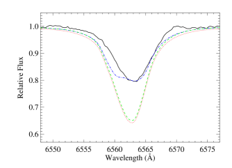
Figure 8: The mean observed ${\rm H}{\alpha}$ profile of $\xi$ Per (solid, black) is well-fitted by a wind model that has the low, X-ray derived mass-loss rate, of $2.2\times 10^{-7}$ ${\mathrm{M_{\sun}~{}{\mathrm{y}r^{-1}}}}$, and $f_{\rm cl}=20$ with a clumping onset, $R_{\rm cl}$, just above the photosphere (dash-dot, blue). Neither an unclumped model (dotted, red) nor a model with $f_{\rm cl}=20$ but a clumping onset of $R_{\rm cl}=1.3$ ${R_{\ast}}$ (dashed, green) fits the data.

To demonstrate this technique, we fit the ${\rm H}{\alpha}$ line (mean profile) measured in one sample star, $\xi$ Per, accounting for optically thin clumping using the synthesis technique developed by Puls et al. (2006) and Sundqvist et al. (2011). Fig. 8 shows several model profiles computed using our X-ray derived mass-loss rate. Models without clumping or with clumping that starts well above the photosphere fail to produce enough ${\rm H}{\alpha}$ emission, but a model with a clumping factor of $f_{\rm cl}=20$ and a clumping onset radius immediately above the photosphere does reproduce the observed ${\rm H}{\alpha}$ emission level. This clumping factor is completely consistent with the smooth-wind ${\rm H}{\alpha}$ mass-loss rate measured by Repolust et al. (2004) when using the scaling law in the previous paragraph. The big difference between the dash-dotted (blue) curve and the dashed (green) curve in Fig. 8 shows that the ${\rm H}{\alpha}$ wind emission in $\xi$ Per originates almost entirely in layers just above the photosphere. A similar result was found for HD 93129A (Cohen et al., 2011), where a radially constant clumping factor of $f_{\rm cl}=12$ with an onset just above the photosphere fits the ${\rm H}{\alpha}$ data along with the X-ray-derived mass-loss rate.

Although the profile fitting presented here is, like any diagnostic technique, subject to various systematic effects, we have quantified those effects and find that they are generally on the order of a few tens of per cent. Uncertainties in the wind opacity, which must be modeled in order to derive a mass-loss rate from an ensemble of $\tau_{\ast}$ values, may be the biggest source of error. But although radial variations within a given wind, and uncertainty about the ionization state and detailed elemental abundances contribute modestly to the systematic errors, the biggest wind opacity uncertainty arises from uncertainty about the overall metallicity of the wind. The opacity is directly proportional to the metallicity and, indeed, using a solar abundance wind opacity model, as we do in this study, has led us to reduce the mass-loss rate estimate of the canonical O supergiant, $\zeta$ Pup, from $3.5\times 10^{-6}$ ${\mathrm{M_{\sun}~{}{\mathrm{y}r^{-1}}}}$ (Cohen et al., 2010a) to $1.8\times 10^{-6}$ ${\mathrm{M_{\sun}~{}{\mathrm{y}r^{-1}}}}$. This value is very close to the newly derived values of $2.1\times 10^{-6}$ ${\mathrm{M_{\sun}~{}{\mathrm{y}r^{-1}}}}$ from the analysis of hydrogen lines in the near-IR (Najarro et al., 2011), and of $2.0\times 10^{-6}$ ${\mathrm{M_{\sun}~{}{\mathrm{y}r^{-1}}}}$ from an optical and UV analysis (Bouret et al., 2012), while the global X-ray modeling of Hervé et al. (2013) finds a modestly higher value of $3.5\times 10^{-6}$ ${\mathrm{M_{\sun}~{}{\mathrm{y}r^{-1}}}}$. Najarro et al. (2011) also includes our programme star $\epsilon$ Ori, for which those authors find $\dot{M}=4.3\times 10^{-7}$ ${\mathrm{M_{\sun}~{}{\mathrm{y}r^{-1}}}}$. That value is bracketed by our two values, the higher of which accounts for resonance scattering.

For the EWS sources in our sample, the fits to the X-ray emission lines also provide information about the spatial distribution and kinematics of the shock-heated wind plasma. In general, we find consistency with models in which the bulk wind and the embedded X-ray plasma have the same kinematics, described by the standard beta wind velocity law, with terminal velocities given by optical and UV diagnostics holding for the X-ray plasma as well as the bulk wind. The shock onset parameter, ${R_{\mathrm{o}}}$, is consistent with ${R_{\mathrm{o}}}\approx 1.5$ ${R_{\ast}}$, or a little less, which is in line with published 1D and 2D numerical simulations of the instability (Feldmeier et al., 1997; Runacres & Owocki, 2002; Dessart & Owocki, 2003, 2005). However, recent wind structure simulations that account for both sound-wave driven excitation of the wind instability and limb darkening, do show more structure near the base of the wind, and certainly well below $r=1.5$ ${R_{\ast}}$ (Sundqvist & Owocki, 2013). But the role of such inner wind structure for the onset of X-ray emission is not yet clear. To reliably predict the X-ray emission from clump-clump collisions, which is likely to be the dominant mode of Line Deshadowing Instability (LDI)-induced EWS X-ray emission (Feldmeier et al., 1997), may require fully 3-D simulations of clump formation.

From a diagnostic perspective, the ${R_{\mathrm{o}}}$ parameter is governed to a large extent by the line widths and thus the kinematics of the X-ray plasma. If X-ray emitting plasma near the wind base actually does exist, but is moving systematically faster than the velocity predicted by the beta law, then our modeling technique would likely overestimate the value of ${R_{\mathrm{o}}}$. It should be kept in mind that there is no intrinsic limitation to the pre-shock flow speed at small radii, as the nature of the LDI is to rapidly accelerate a small fraction of the line-driven wind mass to higher-than-ambient velocities. Another factor to consider is that different lines, sensitive to plasma of different temperatures, may form in different spatial locations (e.g. Hervé et al. 2013). There is some indication from the ${R_{\mathrm{o}}}$ results shown in Fig. 5 that longer wavelength lines, which tend to arise in relatively cooler plasma, form farther out in the wind, and so perhaps some of the shorter wavelength lines, indicative of plasma with temperatures approaching or exceeding $10^{7}$ K, do form at smaller radii, consistent with the base wind shocks seen in the simulations presented in Sundqvist & Owocki (2013).

Regardless of the X-ray shock onset constraints, the consistent ${\rm H}{\alpha}$ and X-ray fitting seems to require – now for $\xi$ Per, too, as shown in Fig. 8, in addition to HD 93129A and $\zeta$ Pup – that clumping begins very close to the photosphere. It is possible for the LDI to produce clumping without also producing significant X-ray emission if the shocks are not strong enough to heat the wind plasma to more than $10^{6}$ K. It is also quite possible that the clumping in O stars begins already in the photosphere, perhaps due to the radiation-driven magneto-acoustic instability (Fernandez & Socrates, 2013). Future simulations will have to address these issues of clump formation and X-ray production in the context of the LDI.

Unfortunately, it is unlikely that many more O stars will be observed at high X-ray spectral resolution in the near future, as the X-ray brightest O stars in the sky are all in the current sample, and as we showed, detailed spectral analysis requires several thousand counts in the Chandra gratings. However, wind absorption of X-rays has an effect on the broad-band X-ray emission in addition to the emission lines, and modeling the global thermal emission spectrum in conjunction with the broad-band wind absorption holds promise for making mass-loss rate measurements (Leutenegger et al., 2010). In fact, this technique has already been applied to HD 93129A and gives results consistent with the line profile fitting approach we use in this paper (Cohen et al., 2011).

In summary, then, the new findings presented in this paper include: (1) mass-loss rates can be determined from X-ray line profile shapes without having to correct for optically thin clumping; and (2) this clumping-insensitive diagnostic finds mass-loss rates that are on average a factor of 3 lower than the theoretical rates of Vink et al. (2000); but (3) in the case of $\zeta$ Oph, which is a previously determined weak-wind star, the mass-loss rate discrepancy is closer to two orders of magnitude; (4) the spatial distribution of the X-ray plasma and its kinematics is roughly consistent with the predictions of numerical simulations of these O star winds; (5) clumping that affects ${\rm H}{\alpha}$ begins very close to the photosphere while the X-ray emission onset is farther out in the wind; and finally (6) a perhaps surprising number of programme stars seem subject to contamination by CWS X-ray emission, even in some cases where the overall X-ray emission is neither unusually strong nor unusually hard.

References

- Asplund et al. (2009) Asplund M., Grevesse N., Sauval A. J., Scott P., 2009, ARAA, 47, 481
- Bagnuolo et al. (2001) Bagnuolo W. G., Riddle R. L., Gies D. R., Barry D. J., 2001, ApJ, 554, 362
- Barker & Brown (1974) Barker P. K., Brown T., 1974, ApJ, 192, L11
- Blumenthal et al. (1972) Blumenthal G.R., Drake G.W.F., Tucker W.H., 1972, ApJ, 172, 205
- Bouret et al. (2012) Bouret J. C., Hillier D. J., Lanz T., Fullerton A. W., 2012, A&A, 544, 67
- Bouret et al. (2005) Bouret J. C., Lanz T., Hillier D. J., 2005, A&A, 438, 301
- Canizares et al. (2005) Canizares C. R., et al., 2005, PASP, 117, 1144
- Cash (1979) Cash W., 1979, ApJ, 228, 939
- Cassinelli et al. (2001) Cassinelli J. P., Miller N. A., Waldron W. L., MacFarlane J. J., Cohen D. H., 2001, ApJ, 554, L55
- Cohen et al. (2011) Cohen D. H., Gagné M., Leutenegger M. A., MacArthur J. P., Wollman E. E., Sundqvist J. O., Fullerton A. W., Owocki S. P., 2011, MNRAS, 415, 3354
- Cohen et al. (2008) Cohen D. H., Kuhn M. A., Gagné M., Jensen E. L. N., Miller N. A., 2008, MNRAS, 386, 1855
- Cohen et al. (2006) Cohen D. H., Leutenegger M. A., Grizzard K. T., Reed C. L., Kramer R. H., Owocki S. P., 2006, MNRAS, 368, 1905
- Cohen et al. (2010a) Cohen D. H., Leutenegger M. A., Wollman E. E., Zsargó J., Hillier D. J., Townsend R. H. D., Owocki S. P., 2010, MNRAS, 405, 2391
- Cohen et al. (2010b) Cohen D. H., Wollman E. E., Leutenegger M. A., 2010, in Neiner C., Wade G., Meynet G., Peters G. eds, IAU Symposium 272. Cambridge University Press, Cambridge, p. 348
- Conti & Ebbets (1977) Conti P. S., Ebbets D., 1977, ApJ, 213, 438
- Corcoran et al. (2013) Corcoran M., et al., 2013, in Massive Stars from Alpha to Omega, 60
- De Becker et al. (2006) De Becker M., Rauw G., Sana H., Pollock A. M. T., Pittard J. M., Blomme R., Stevens I. R., van Loo S., 2006, MNRAS, 371, 1280
- De Jong et al. (2001) de Jong J. A., et al., 2001, A&A, 368, 601
- Dessart & Owocki (2003) Dessart L., Owocki S. P., 2003, A&A, 406, L1
- Dessart & Owocki (2005) Dessart L., Owocki S. P., 2005, A&A, 437, 657
- Feldmeier et al. (1997) Feldmeier A., Puls J., Pauldrach A. W. A., 1997, A&A, 322, 878
- Fernandez & Socrates (2013) Fernandez R., Socrates A., 2013, ApJ, 767, 144
- Fullerton et al. (2006) Fullerton A. W., Massa D. L., Prinja R. K., 2006, ApJ, 637, 1025
- Gabriel & Jordan (1969) Gabriel H. A., Joran C., 1969, MNRAS, 145, 241
- Gagné et al. (2011) Gagné M., et al., 2011, ApJS, 194, 5
- Gagné et al. (2012) Gagné M., Fehon G., Savoy M. R., Cartagena C. A., Cohen D. H., Owocki S. P., 2012, in Drissen L., Robert C., St. Louis N., Moffat A. F. J. eds, ASP Conf. Ser. Vol. 465, Four Decades of Research in Massive Stars. Astronomical Society of the Pacific, San Francisco, p. 301 (arXiv:1205.3510)
- Halbedel (1985) Halbedel E. M., 1985, PASP, 97, 434
- Haser (1995) Haser S. M., 1995, Ph.D. thesis, Universitäts-Sternwarte der Ludwig-Maximillian Universität, München
- Henley et al. (2003) Henley D. B., Stevens I. R., Pittard J. M., 2003, MNRAS, 346, 773
- Henley et al. (2005) Henley D. B., Stevens I. R., Pittard J. M., 2005, MNRAS, 356, 1308
- Hervé et al. (2013) Hervé A., Rauw G., Nazé Y., 2013, A&A, 551, 83
- Hervé et al. (2012) Hervé A., Rauw G., Nazé Y., Foster A., 2012, ApJ, 748, 89
- Hillier & Miller (1998) Hillier D. J., Miller D. L., 1998, A&A, 496, 407
- Hoogerwerf et al. (2001) Hoogerwerf R., de Bruijne J. H. J., de Zeeuw P. T., 2001, A&A, 365, 49
- Huenemoerder et al. (2012) Huenemoerder D. P., Oskinova L. M., Ignace R., Waldron W. L., Todt H., Hamaguchi K., Kitamoto S., 2012, ApJ, 756, 34
- Hummel et al. (2000) Hummel C. A., White N. M., Elias N. M., Hajian A. R., Nordgren T. E., 2000, ApJ, 540, L91
- Kahn et al. (2001) Kahn S. M., Leutenegger M. A., Cottam J., Rauw G., Vreux J.–M., den Boggende A. J. F., Mewe R., Güdel M., 2001, A&A, 365, L312
- Kramer et al. (2003) Kramer R. H., Cohen D. H., Owocki S. P., 2003, ApJ, 592, 532
- Lanz & Hubeny (2003) Lanz T., Hubeny I., 2003, ApJS, 146, 417
- Leutenegger et al. (2013) Leutenegger M. A., Cohen D. H., Sundqvist J. O., Owocki S. P., 2013, ApJ, 770, 80
- Leutenegger et al. (2010) Leutenegger M. A., Cohen D. H., Zsargó J., Martell E. M., MacArthur J. P., Owocki S. P., Gagné M., Hillier D. J., 2010, ApJ, 719, 1767
- Leutenegger et al. (2007) Leutenegger M. A., Owocki S. P., Kahn S. M., Paerels F. B. S., 2007, ApJ, 659, 642
- Leutenegger et al. (2006) Leutenegger M. A., Paerels F. B. S., Kahn S. M., Cohen D. H., 2006, ApJ, 650, 1096
- MacFarlane et al. (1991) MacFarlane, J. J., Cassinelli J. P., Welsh B. Y., Vedder P. W., Vallerga J. V., Waldron W. L., 1991, ApJ, 380, 564
- MacFarlane et al. (1994) MacFarlane, J. J., Cohen D. H., Wang P., 1994, ApJ, 437, 351
- Mahy et al. (2012) Mahy L., Gosset E., Sana H., Damerdji Y., De Becker M., Rauw G. Nischelm C., 2012, A&A, 540, 97
- Marcolino et al. (2009) Marcolino W. L. F., Bouret J.-C., Martins F., Hillier D. J., Lanz T., Escolano C., 2009, A&A, 498, 837
- Markova et al. (2004) Markova N., Puls J., Repolust T., Markov H., 2004, A&A, 413, 693
- Martins et al. (2005) Martins F., Schaerer D., Hillier D. J., 2005, A&A, 436, 1049
- Mauche et al. (2001) Mauche C. W., Liedahl D. A., Fournier M. B., 2001, ApJ, 560, 992
- Massa (1995) Massa D., 1995, ApJ, 438, 376
- Miller et al. (2002) Miller N. A., Cassinelli J. P., Waldron W. L., MacFarlane J. J., Cohen D. H., 2002, ApJ, 577, 951
- Mokiem et al. (2005) Mokiem M. R., de Koter A., Puls J., Herrero A., Najarro F., Villamariz M. R., 2005, A&A, 441, 711
- Najarro et al. (2011) Najarro F., Hanson M. M., Puls J., 2011, A&A, 535, 32
- Nazé et al. (2010) Nazé Y., Rauw G., ud-Doula A., 2011, A&A, 510, 59
- Nelan et al. (2004) Nelan E. P., Walborn N. R., Wallace D. J., Moffat A. F. J., Makidon R. B., Gies D. R., Panagia N., 2004, AJ, 128, 323
- Nelan et al. (2010) Nelan E. P., Walborn N. R., Wallace D. J., Moffat A. F. J., Makidon R. B., Gies D. R., Panagia N., 2010, AJ, 139, 2714
- Nichols et al. (2013) Nichols J., et al., 2013, in Massive Stars from Alpha to Omega, 88
- Niemela & Gamen (2005) Niemela V. S., Gamen R. C., 2005, MNRAS, 356, 974
- Oskinova et al. (2006) Oskinova L., Feldmeier A., Hamann W.–R., 2006, MNRAS, 372, 313
- Oskinova et al. (2007) Oskinova L., Hamann W.–R., Feldmeier A., 2007, A&A, 476, 1331
- Owocki (2008) Owocki S. P., 2008, in Clumping in Hot Star Winds, eds. W.-R. Hamann, A. Feldmeier, & L. M. Oskinova, 121
- Owocki & Cohen (2001) Owocki S. P., Cohen D. H., 2001, ApJ, 559, 1108
- Owocki & Cohen (2006) Owocki S. P., Cohen D. H., 2006, ApJ, 648, 565
- Owocki et al. (2013) Owocki S. P., Sundqvist J. O., Cohen D. H., Gayley K. G., 2013, ApJ, 429, 3379
- Petit et al. (2013) Petit V., et al., 2013, MNRAS, 429, 398
- Pittard & Parkin (2010) Pittard J. M., Parkin E. R., 2010, MNRAS, 403, 1657
- Press et al. (2007) Press W. H., Flannery B. P., Teukolsky S. A., Vetterling W. T., 2007, Numerical Recipes, 3rd edition. Cambridge University Press, Cambridge
- Puls et al. (2006) Puls J., Markova N., Scuderi S., Stanghellini C., Taranova O. G., Burnley A. W., Howarth I. D., 2006, A&A, 454, 625
- Puls et al. (2008) Puls J., Vink J. S., Najarro F., 2008, A&A Rev., 16, 209
- Rauw et al. (2005) Rauw G., Sana H., Gosset E., De Becker M., Arias J., Morrell N., Eenens P., Stickland D., 2005, in “Massive Stars and High-Energy Emission in OB Associations,” eds. G. Rauw, Y. Nazé, R. Blomme, & E. Gosset, Liege: JENAM, 85
- Rauw et al. (2002) Rauw G., Blomme R., Waldron W. L., Corcoran M. F., Pittard J. M., Pollock A. M. T., Runacres M. C., Sana H., Stevens I. R., Van Loo S., 2002, A&A, 394, 993
- Repolust et al. (2004) Repolust T., Puls J., Herrero A., 2004, A&A, 415, 349
- Richichi & Percheron (2002) Richichi A., Percheron I., 2002, A&A, 386, 492
- Rivinius et al. (2011) Rivinius T., Hummel C. A., Stahl O., 2011, IAUS, 272, 539
- Runacres & Owocki (2002) Runacres M. C., Owocki S.P., 2002, A&A, 381, 1015
- Russell et al. (2013) Russell C. M. P., Okazaki A. T., Owocki S. P., Corcoran M. F., Madura T. I., Leyder J. C., Hamaguchi K., in Massive Stars from Alpha to Omega, 182
- Sana et al. (2011) Sana H., Le Bouquin J.-B., De Becker M., Berger J.-P., de Koter A., Mérand A., 2011, ApJ, 740, L43
- Sana et al. (2013) Sana H., Le Bouquin J.-B., Mahy L., Absil O., De Becker M., Gosset E., 2013, A&A, 553, 131
- Searle et al. (2008) Searle S. C., Prinja R. K., Massa D., Ryan R., 2008, A&A, 481, 777
- Skinner et al. (2005) Skinner S. L., Zhekov S. A., Palla F., Barbosa C. L. D. R., 2005, MNRAS, 361, 191
- Skinner et al. (2008) Skinner S. L., Sokal K. R., Cohen D. H., Gagné M., Owocki S. P., Townsend R. D., 2008, ApJ, 683, 796
- Sota et al. (2008) Sota A., Maíz Apellániz J., Walborn N. R., Shida R. Y., 2008, Rev. Mex., 33, 56
- Sundqvist & Owocki (2013) Sundqvist J. O., Owocki S. P., 2013, MNRAS, 428, 1837
- Sundqvist et al. (2012) Sundqvist J. O., Owocki S. P., Cohen D. H., Leutenegger M. A., Townsend R. H. D., 2012, MNRAS, 420, 1553
- Sundqvist et al. (2010) Sundqvist J. O., Puls J., Feldmeier A., 2010, A&A, 510, 11
- Sundqvist et al. (2011) Sundqvist J. O., Puls J., Feldmeier A., Owocki S. P., 2011, A&A, 528, 64
- Townsley et al. (2011) Townsley L., et al., 2011, ApJS, (arXiv:1102.4779)
- Vink et al. (2000) Vink J., de Koter A., Lamers H. J. G. L. M., 2000, A&A, 362, 295
- Walborn et al. (2009) Walborn N. R., Nichols J. S., Waldron W. L., 2009, ApJ, 703, 633
- Waldron & Cassinelli (2007) Waldron W. L., Cassinelli J. P., ApJ, 668, 456
- Waldron et al. (2004) Waldron W. L., Cassinelli J. P., Miller N. A., MacFarlane J. J., Reiter J. C., 2004, ApJ, 616, 542
- Westbrook et al. (2008) Westbrook O. W., et al., 2008, ApJS, 176, 218
- Zhekov & Palla (2007) Zhekov S. A., Palla F., 2007, MNRAS, 382, 1124