Gravitational Lens Recovery with Glass: Measuring the mass profile and shape of a lens
Abstract
We use a new non-parametric gravitational modelling tool – Glass – to determine what quality of data (strong lensing, stellar kinematics, and/or stellar masses) are required to measure the circularly averaged mass profile of a lens and its shape. Glass uses an under-constrained adaptive grid of mass pixels to model the lens, searching through thousands of models to marginalise over model uncertainties. Our key findings are as follows: (i) for pure lens data, multiple sources with wide redshift separation give the strongest constraints as this breaks the well-known mass-sheet or steepness degeneracy; (ii) a single quad with time delays also performs well, giving a good recovery of both the mass profile and its shape; (iii) stellar masses – for lenses where the stars dominate the central potential – can also break the steepness degeneracy, giving a recovery for doubles almost as good as having a quad with time delay data, or multiple source redshifts; (iv) stellar kinematics provide a robust measure of the mass at the half light radius of the stars that can also break the steepness degeneracy if the Einstein radius ; and (v) if , then stellar kinematic data can be used to probe the stellar velocity anisotropy – an interesting quantity in its own right. Where information on the mass distribution from lensing and/or other probes becomes redundant, this opens up the possibility of using strong lensing to constrain cosmological models.
keywords:
gravitational lensing: strong, methods: numerical, methods: statistical1 Introduction
Strong gravitational lenses are rare. Since the discovery of the first lens Q0957+561 (Walsh et al., 1979), just have been discovered to date111See, e.g., http://masterlens.astro.utah.edu for a catalogue.. However, this number is expected to increase to several thousand over the next ten years as new surveys, both ground-based222http://pan-starrs.ifa.hawaii.edu,333http://www.darkenergysurvey.org and space-based444http://www.euclid-ec.org – together with a community of citizen-science volunteers examining the image data for candidates555http://spacewarps.org – come online.
Since lensing depends only on gravity, strong lenses offer a unique window onto dark matter and cosmology (Bartelmann, 2010; Amendola et al., 2013). However, extracting dark matter properties or cosmological constraints from these lensing data will require sophisticated modelling. In particular, with an unprecedented data set imminent, it is prudent to look again at systematic errors in the lens models to determine what quality of data (in particular complementary data from stellar/gas kinematics, lens time delays and/or stellar mass constraints) are required to address problems of interest. It is towards that goal that this present work is directed.
To see why lens modelling details are of crucial importance, let us recall the essential quantities that appear in lensing (see also §2 for a more detailed exposition). First we have the distances. Let , , be the angular-diameter distances to the lens, source, and from lens to source; these are all proportional to but have factors that depend on the particular choice of cosmology666Here, is the speed of light in vacuo and is the Hubble parameter.. Typically:
| (1) |
where is the redshift of the lens. For multiple images, the sky-projected density must exceed the critical lensing density in some region:
| (2) |
where is Newton’s gravitational constant. The angular separation between the lensed images is of order the Einstein radius , which is related to the mass by:
| (3) |
where (with the projected mass enclosed within ) is the gravitational radius. If the source is a quasar or otherwise rapidly variable, a time delay in the variability will be present where:
| (4) |
So in principle, one can not only measure the mass of the lens, one can use the dependence on the cosmology-dependent factors to extract the cosmological model and all its parameters. Zwicky (1937) drew attention to the former, and Refsdal (1964, 1966) pointed out the latter, all long before lenses were discovered. The difficulty with actually doing this, however, became apparent soon after the discovery of the first lens by Walsh et al. (1979). In the first ever paper on lens modelling, Young et al. (1981) found that many plausible mass distributions could reproduce the data.
Young et al. (1981) were remarkably prescient about the subsequent development of lens modelling. First, they introduced the technique of choosing a parametric form for the lensing mass and then fitting for the parameters, which is still the most common strategy (see for example Keeton, 2010; Kneib & Natarajan, 2011). Second, they pointed out the non-uniqueness of lens models – lensing degeneracies. Third, they suggested combining lensing data with stellar kinematics and X-rays, to reduce the effect of the degeneracies. Later work, as well as following up these suggestions, has introduced some further new ideas. Five of these are important for the present work:
-
1.
Free-form modelling: In ‘free-form’ or non-parametric modelling, there is no specified parametric form for the mass distribution. There are still assumptions (or priors) on the mass distribution, such as smoothness or being centrally concentrated (Saha & Williams, 1997; Diego et al., 2005; Merten et al., 2009; Coe et al., 2010) but these are much less restrictive than parametric forms. A particularly elegant prior is implemented by Liesenborgs et al. (2006), requiring that the mass distribution to be non-negative and no extra images allowed. To be concrete, we define from here on:
Non-parametric, or ‘free-form’ more parameters than data constraints (i.e. deliberately under-constrained)
Being under-constrained, it is then necessary to explore model degeneracies rather than finding a single ‘best-fit’ solution. Free-form models are more commonly used with cluster lenses (Saha et al., 2006; Saha & Read, 2009; Merten et al., 2009; Sendra et al., 2014), but can be used with galaxy lenses as well, where their less restrictive assumptions can be important. For example, in time-delay galaxy lenses, parametric model measures of the Hubble parameter have historically been at tension with independent measures (e.g., Kochanek, 2002a, b); these are resolved once the less restrictive assumptions of free-form models are permitted (Read et al., 2007). Hybrid methods, using a mass grid on top a parametric model, have also been explored (e.g., Vegetti et al., 2010).
-
2.
Model ensembles: Model ensembles, exploring a diverse range of possible mass distributions that nonetheless all fit the data, are a way of combating the non-uniqueness of models. Such ensembles are possible in parametric models (e.g., Bernstein & Fischer, 1999; Jullo et al., 2010; Richard et al., 2014; Johnson et al., 2014; Coe et al., 2014), but are more common in free-form models, where – since such models are deliberately under-constrained – they become vital (Williams & Saha, 2000; Saha & Read, 2009; Lubini & Coles, 2012).
-
3.
Stellar kinematic constraints: This was first suggested by Treu & Koopmans (2002) as a means to break lensing degeneracies. The idea is that stellar kinematics can provide an independent estimate of the Einstein radius, via the virial theorem:
(5) where is the line of sight stellar velocity dispersion, and the above relation becomes exact for isothermal lenses. This can then be used to probe cosmological parameters if lenses are known to be isothermal (e.g., Collett et al., 2012); or to break the steepness degeneracy in the more general situation (see §2.3). The technique has since been applied to many lenses (e.g., Koopmans et al., 2006; Bolton et al., 2008). Going further, the use of two-dimensional kinematics (Barnabè et al., 2011) is especially interesting.
-
4.
Stellar mass constraints: The stellar mass in a lens can be inferred from photometry and compared with the total mass (e.g., Keeton et al., 1998; Kochanek et al., 2000; Rusin et al., 2003; Ferreras et al., 2005, 2008; Leier et al., 2011). Since the inferred stellar mass depends on the assumed IMF, lenses in which stellar mass dominates can be used to derive upper bounds on the stellar (Ferreras et al., 2010). Lower bounds on stellar have also recently been claimed by fitting CDM semi-analytic models to the tilt of the fundamental plane (Dutton et al., 2013).
-
5.
Testing modelling strategies: Using mock data to see how well a given model can recover simulated lenses is increasingly being recognised as essential. Simple blind tests have appeared in earlier work (for example, Figure 2 in Williams & Saha, 2000), but more recently, tests against dynamically simulated galaxies or clusters are favoured (Read et al., 2007; Liesenborgs et al., 2007; Merten et al., 2009; Barnabè et al., 2009; Coe et al., 2010).
There are three further key modelling ideas in the literature that we will not touch upon in this present work: to use X-ray intensity and temperature profiles as a mass constraint (e.g., Newman et al., 2013); and to model multiple lenses simultaneously, with one or more cosmological parameters variable but shared between the lenses. This latter strategy has been used to constrain from time delay lenses (Saha et al., 2006; Coles, 2008; Paraficz & Hjorth, 2010) and recently the cosmological parameters as well (Sereno & Paraficz, 2014). Third, it is in principle possible to estimate the parameters even from a single lens, if there are lensed sources at multiple redshifts (Lubini et al., 2014) or by using additional priors (Jullo et al., 2010; Suyu et al., 2014).
In this paper, we introduce a new non-parametric lens modelling framework – Glass (Gravitational Lensing AnalysiS Software). This shares some aspects with an earlier code PixeLens (Saha & Williams, 2004; Coles, 2008). However, Glass – which contains all new code written from the ground up – significantly improves upon PixeLens in several key ways:
-
1.
At the heart of Glass is a new uniform sampling algorithm for high dimensional spaces (Lubini & Coles, 2012). This allows for large ensembles of models to be efficiently generated.
-
2.
Glass provides a modular framework that allows new priors to be added and modified easily.
-
3.
The basis functions approximating a model can be easily changed (in this paper, we assume pixels as in PixeLens).
-
4.
With so many models in the final ensemble, we can afford to apply non-linear constraints (for example stellar kinematic data; or the removal of models with spurious extra images) to accept/reject models in a post-processing step.
-
5.
The central region of the mass map can have a higher resolution to more efficiently capture steep models.
-
6.
Stellar density can be used as an additional constraint on the models.
-
7.
Point or extended mass objects can be placed in the field.
As a first application, we use Glass on mock data to determine which combination of lensing, stellar mass and/or stellar kinematic constraints best constrain the projected mass profile and shape of a gravitational lens. We will apply Glass to real lens data in a series of forthcoming papers.
This paper is organised as follows. In §3, we describe the Glass code. In §2, we review the key elements of lensing theory, stellar population synthesis, and stellar dynamics we will need. In §4, we describe our mock data. In §5, we present our results from applying Glass to these mock data. Finally, in §6 we present our conclusions.
2 Theory
2.1 Lensing essentials
In the following summary, we follow Blandford & Narayan (1986) with some differences in notation, in particular putting back the speed of light and the gravitational constant .
The lens equation:
| (6) | ||||
maps an observed image position to a source position . Using the thin lens approximation, the lens can be thought of as a projected surface density which diverts the path of a photon instantaneously through the bending angle . The factors, as in the previous section, are angular diameter distances, which depend on the cosmological density-parameters , the redshifts of the lens and the source, and the Hubble parameter , thus
| (7) |
and , . One way to understand the lens equation is via Fermat’s principle. We can think of light as travelling only along extremum paths where lensed images occur. Such paths occur at the extrema of the photon arrival time that depends on the geometric path the photon takes and the general relativistic gravitational time dilation due to a thin lens at redshift :
| (8) | ||||
We can simplify the above equation by introducing a dimensionless time and density :
| (9) |
and hence rewrite Eq. (8) as:
| (10) |
The scaled arrival time is like a solid angle. It is of order the area (in steradians) of the full lensing system. The expression is of order the image-separation squared, and the other terms are of similar size. For this reason, is convenient to measure in arcsec2.
Lensing observations provide information only at where there are images. Hence, the arrival-time surface is not itself observable. Its usefulness lies in that observables can be derived from it. An image observed at implies that . A measurement of time delays between images at and implies that is known. Interestingly, both these types of observations give constraints that are linear in and .
The rather complicated dependence of lensing observables on the mass distribution has an important consequence: very different mass distributions can result in similar observables. This is the phenomenon of lensing degeneracies. While the non-uniqueness of lens models noted by Young et al. (1981) already hinted at degeneracies, their existence was first derived by Falco et al. (1985). The most important is the so-called mass-sheet degeneracy, which is that image positions remain invariant if is multiplied by an arbitrary constant. This corresponds to rescaling the surface density at the images . In fact there are infinitely many degeneracies (Saha, 2000) because any transformation of the arrival-time surface away from the images has no effect on the lensing observables. In particular, there are degeneracies that involve the shape of the mass distribution (Saha & Williams, 2006; Schneider & Sluse, 2014). Degeneracies tend to be suppressed if there are sources at very different redshifts or ‘redshift contrast’ (AbdelSalam et al., 1998; Saha & Read, 2009), because the presence of different factors of in the image plane makes it more difficult to change the mass distribution and the arrival-time surface without affecting the lensing observables. But degeneracies are still present with multiple source redshifts (Liesenborgs et al., 2008; Schneider, 2014).
2.2 Stellar populations
For many galaxy lenses, the gravitational potential in the inner region is dominated by the stellar mass. Stellar mass can be estimated by combining photometry and colours with models of the stellar populations. Such estimates are reasonably robust, even if the star-formation history is very uncertain: given a stellar-population model (such as Bruzual & Charlot, 2003) and an initial mass function (IMF), the stellar mass can be inferred to 0.1 to 0.2 dex using just two photometric bands (see, e.g., Figure 1 in Ferreras et al., 2008). By comparing the lensing-mass and stellar-mass profiles in elliptical galaxies, it is possible to extract the radial dependence of the baryonic vs dark-matter fraction (Ferreras et al., 2005, 2008; Leier et al., 2011).
The major uncertainty at present in the stellar mass is probably the IMF. In the lensing galaxy of the Einstein Cross, the IMF cannot be much more bottom-heavy than Chabrier (2003), because otherwise the stellar mass would exceed the lensing mass Ferreras et al. (2010). More massive galaxies, however, do appear to have more of their stellar mass in low-mass stars. This is indicated by molecular spectral features characteristic of low mass stars (Cenarro et al., 2004; Conroy & van Dokkum, 2012; Ferreras et al., 2013). The Chabrier (2003) IMF would, however, still provide a robust lower limit on the stellar mass and hence, also a limit on the total mass. Accordingly, Glass allows a constraint of the form
| (11) |
on the total mass.
2.3 Stellar kinematics
Another useful constraint follows from the velocity of stars within the lensing galaxy. Assuming spherical symmetry, stars obey the projected Jeans equations (e.g., Binney & Tremaine, 2008):
| (12) |
| (13) |
where is the projected velocity dispersion of the stars as a function of projected radius ; is the surface density of the stars; is the three dimensional stellar density; are the radial and tangential velocity dispersions, respectively; is the velocity anisotropy (here assumed to be constant, and not to be confused with from lensing); is Newton’s gravitational constant; and is the mass profile that we would like to measure. By convention, we always write for a projected radius, and for a 3D radius.
It is immediately clear from Eq. (12) that, even assuming spherical symmetry, we have a degeneracy between the enclosed mass profile and the velocity anisotropy . This can be understood intuitively since measures the relative importance of radial versus circular orbits and is intrinsically difficult to constrain given only one component of the velocity vector for each star. Nonetheless, can be constrained given sufficiently many stars, since radial Doppler velocities sample eccentric orbits as and tangential orbits as (e.g., Wilkinson et al., 2002). It can also be estimated if an independent measure of is available – for example coming from strong lensing.
While is difficult to measure from stellar kinematics alone, the mass within the half light radius is robustly recovered (e.g., Walker et al., 2009; Wolf et al., 2010; Agnello & Evans, 2012) since stellar systems in dynamic quasi-equilibrium obey the virial theorem (equation 5). This means that stellar kinematics can break the steepness degeneracy if , where is the physical Einstein radius. We test this expectation in §5.
3 Numerical Methods
3.1 A new lens modelling framework: Glass
Glass is the Gravitational Lensing AnalysiS Software. It extends and develops some of the concepts from the free form modelling tool PixeLens (Saha & Williams, 2004; Coles, 2008), but with all new code. The most compute intensive portion was written in C but Python was chosen because of its flexibility as a language and for its large scientific library support. The flexibility allows Glass to have quite sophisticated behavior while at the same time simplifying the user experience and reducing the overall development time. One of the striking features is that the input file to Glass is itself a Python program. Understanding Python is not necessary for the most basic use, but this allows a user to build complex analysis of a model directly into the input file. Glass may furthermore be used as an external library to other Python programs. The software is freely available for download or from the first author.777http://www.jpcoles.com
The key scientific and technical improvements are:
-
1.
A new uniform sampling algorithm for high dimensional spaces.
At the heart of Glass lies a new algorithm for sampling the high dimensional linear space that represents the modelling solution space. This algorithm was described and tested in Lubini & Coles (2012); it is multi-threaded allowing it to run efficiently on many-cored machines.
-
2.
A modular framework that allows new priors to be added and modified easily.
Each prior is a simple function that adds linear constraints that operate on either a single lens object or the entire ensemble of objects. Glass comes with a number of useful priors (the default ones will be described in §3.3), but a user can write their own directly in the input file, or by modifying the source code.
-
3.
The basis functions approximating a model can be changed.
Glass currently describes the lens mass as a collection of pixels, but the code has been designed to support alternative methods. In particular, there are future plans to develop a module using Bessel functions. This will require a new set of priors that operate on these functions.
-
4.
Non-linear constraints can be imposed in an automated post-processing step.
Once Glass has generated an ensemble of models given the linear constraints, any number of post processing functions can be applied. Not only can these functions be used to derive new quantities from the mass models, they can also be used as a filter to accept or reject a model based on some non-linear constraint. For example, we can reject models that have spurious extra images (§3.6), or models that do not match stellar kinematic constraints (§3.7). The plotting functions within Glass will correctly display models that have been accepted or rejected.
-
5.
The central region can have a higher resolution to capture steep models.
With the default basis set of pixels, the mass distribution of the lens is described by a uniform grid. However, in the central region of a lensing galaxy where the mass profile may rise steeply, the center pixel uses a higher resolution. This allows the density to increase smoothly but still allow for a large degree of freedom within the inner region without allowing the density to be arbitrarily high.
-
6.
Stellar density can be used as an additional constraint.
The mass in inner regions of galaxies is often dominated by the stellar component which one can estimate using standard mass-to-light models. This data can be added to the potential as described later in §5.3. By using the stellar mass one can place a lower bound on the mass and help constrain the inner most mass profile.
-
7.
Point or extended mass objects can be placed in the field.
A shear term can be added to the potential, as shown later in Eq. (15), to account for mass external to the modelled region. This is useful to capture the gross effects of a distant neighbour, since there is a degeneracy between the ellipticity of a lens and its shear field (the greater the allowed shear, the more circular the lens may be). Glass also allows further analytic potential components to be included. These can be used to model substructure or multiple neighbours close to the main lens. The substructure may have only a small effect if the lens is a single galaxy, but if the lens is a group or cluster then a potential can be added for each of the known member galaxies. A few standard functions are already included in Glass including those for a point mass, a power law distribution, or an isothermal (a particular case of the power law).
3.2 Analysis Tools
Glass is not only a modeling tool but also an analysis engine. Glass provides many functions for viewing and manipulating the computed models. These functions can either be called from a program written by the user or by using the program viewstate.py included with Glass. There is also a tool, lenspick.py for creating a lens, either analytically or from an -body simulation file. To load the simulation data, Glass relies on the Pynbody library (Pontzen et al., 2013) and can thus load any file supported by that package.
3.3 Pixelated models
For this paper, we will restrict ourselves to using a pixelated basis set as used by PixeLens (Saha & Williams, 2004; Coles, 2008), but note that it is straightforward to add other basis function expansions to Glass. The algorithm for generating models in Glass samples a convex polytope in a high dimensional space whose interior points satisfy both the lens equation and other physically motivated linear priors (Lubini & Coles, 2012). A limitation of our sampling strategy is that only linear constraints may be applied when building the model ensemble; however, non-linear constraints can be applied in post-processing (see §3.6 and §3.7). We therefore formulate all of our equations as equations linear in the unknowns. We describe the density distribution as a set of discrete grid cells or pixels and rewrite the potential (Eq. 27) as:
| (14) |
where the sum runs over all the pixels and is the integral of the logarithm over pixel . The exact form for is described in Appendix B. We can find the discretized lens equation by simply taking the gradient of the above equations.
The pixels only cover a finite circular area with physical radius and pixel radius with the central cell centered on the lensing galaxy. To account for any global shearing outside this region from, e.g., a neighboring galaxy, we also add to Eq. (14) two shearing terms:
| (15) |
We can continue adding terms to account for other potentials. For instance, we may want to impose a base potential over the field, or add potentials from the presence of other galaxies in the field. Glass already includes potentials for a point mass or an exponential form, but custom potentials are straightforward to add and can be included directly in the input file. If the stellar density has been estimated we can use this as a lower bound where the stellar potential is a known constant of the form Eq. (14), e.g., for a two-component model.
3.3.1 Priors
The lens equation and the arrival times alone are typically not enough to form a closed volume in the solution space. We therefore require additional linear constraints – priors. Some of these are ‘physical’ in the sense that they are unarguable – for example demanding that the mass density is everywhere positive; others are more subjective, for example demanding that the mass map is smooth over some region. Such ‘regularisation’ priors may be switched off for all or some of the mass map if the data are sufficiently constraining.
The priors built in to Glass are similar to those used in PixeLens (Coles, 2008). The physical priors are always used by default; the regularisation priors are used sparingly – i.e. only if the data are not sufficiently constraining to obtain sensible solutions without them:
Physical priors
-
1.
The density must be non-negative everywhere.
-
2.
Image parity is enforced.
Regularisation priors
-
1.
The local gradient everywhere must point within of the center.
-
2.
The azimuthally averaged density profile must have a slope everywhere .
-
3.
The density is inversion symmetric.
For typical lens data, the regularisation priors are very important for creating physically sensible solutions. Prior (i) demands that the peak in the mass density is at the centre of the mass map. Secondary ‘plateaus’ in the mass map are possible, but not secondary peaks. Note that this prior still successfully allows merging galaxy systems to be correctly captured, provided that the two galaxies are not equally dense in projection (see, for example the PixeLens model of the merger system B1608 in Read et al. 2007); and for the successful detection of ‘meso-structure’ in strong lensing galaxy clusters (Saha et al., 2007). Prior (ii) is arguably a physical prior since a positive slope in the azimuthally averaged density profile would be unstable (e.g., Binney & Tremaine, 2008). Note that this prior does not preclude successful modelling of mergers or substructure unless the total projected mass in substructure is comparable to the projected mass of the host in an azimuthal annulus (Read et al., 2007; Saha et al., 2007). Prior (iii) is only used for doubles that ought to be inversion symmetric and quads where inversion symmetry is clear from the image configuration.
Finally, we remind the reader that all of the regularisation priors can be switched off or changed/improved depending on the data quality available. For clusters, substructure can be explicitly modelled by adding analytic potentials at the known locations of galaxies; furthermore the above priors can be relaxed in regions of the mass map where the data are particularly constraining (for example near the images). We will apply Glass to a host of strong lensing clusters in forthcoming work, where we will explicitly test the prior on mock data that has significant substructure.
3.4 Building the model ensemble
In the simplest form, a single model for a lens is a tuple . A single model represents a single point in the solution space polytope. Using the MCMC sampling strategy described in Lubini & Coles (2012) we uniformly sample this space. Collectively, the sampled models are referred to as an ensemble , where we usually generate models. One can choose to further process these models to impose priors that may be difficult to enforce during the modeling process. For instance, non-linear constraints, or simply filtering of models that do not meet some criteria can be excluded, or weighted against as discussed previously. In this paper, we do not exclude any models and treat all models as equally likely.
The time to generate the model ensemble is mostly a function of the size of the parameter space. The MCMC algorithm has a “warm-up” phase where it estimates the size and shape of each dimension in the solution space. Once this has been completed, the models are sampled very quickly. In fact, there is little difference between generating 1,000 or 10,000 models, although we find little statistical difference after 1,000 models. For the mock lenses, the typical “warm-up” time was about 4s, and the modelling time was 20s using a parallel shared-memory machine with 40 cores. The ability to rapidly generate so many models is what allows us to then accept/reject models to apply non-linear constraints (see §3.6 and §3.7). This is a key advantage over our earlier pixelated strong lens tool PixeLens.
3.5 Raytracing
Glass can also determine the position of images and time delays from particle-based simulation output given a source position . This is used to generate the lens configurations used in the parameter study. The particles are first projected onto a very high resolution grid representing the lens plane. The centers of each of the grid cells are mapped back onto the source plane using Eq. (6). If the location on the source plane is within a user specified of then is accepted and further refined using a root finding algorithm until the distance to is nearly zero. If multiple points converge to an of each other then only one point is taken. Care must be taken that the grid resolution is high enough that the resulting image position error is below the equivalent observational error. Time delays are then calculated in order of the arrival time at each image (Eq. 25).
3.6 Removing models with extra images
While linear constraints are applied in Glass by the nature of the sampling algorithm, non-linear constraints must be applied in post-processing. Models that are inconsistent with such constraints must then be statistically discarded via a likelihood analysis. An example of such a non-linear constraint is the spurious presence of unobserved images. This ‘null-space’ prior was first proposed and explored by Liesenborgs et al. (2006) and found to be extremely powerful. We find that our gradient prior in Glass (see §3.3), performs much of the same function as Liesenborgs et al.’s null-space prior, but some models can still rarely turn up spurious images. We reject these in a post-processing step, where we sweep through the model ensemble applying the ray tracing algorithm described in 3.5.
3.7 A post-processing module for stellar kinematics
Similarly to the null-space constraint (§3.6), stellar kinematic constraints constitute a non-linear prior on the mass map and must be applied in post-processing. We sweep through the model ensemble performing an Abel deprojection to determine from the projected surface density assuming spherical symmetry (e.g., Binney & Tremaine, 2008; Broadhurst & Barkana, 2008):
| (16) | |||||
where
| (17) |
is the projected enclosed mass evaluated at 3D radius ; and .
This de-projection algorithm was tested on triaxial figures in Saha et al. (2006). They found that for triaxialities typical of our current cosmology, the method works extremely well unless the triaxial figure is projected directly along the line of sight such that we see the galaxy or galaxy cluster ‘down the barrel’. Such a situation is unlikely, but in any case avoidable since the resultant figure appears spherical in projection. This leads to the seemingly counter-intuitive result that the kinematic constraints – that rely on the above de-projection – are most secure for systems that do not appear spherical in projection (unless independent data can confirm the three dimensional shape is indeed very round).
We use the deprojected mass to numerically solve Eq. (12) for constant , assuming either or at all radii to bracket the two extremum situations. Where the data are good enough, these two may be distinguished giving dynamical information about . In more typical situations, however, we seek to simply marginalise over the effect of , using the stellar kinematics as a robust measure of (see §2.3).
4 The mock data
We now present a study of four mock galaxies with known analytic forms. These are used to verify that Glass is able to correctly recover the mass profile, and – more importantly – to determine what type and quality of data best constrain the mass profile and shape of a lens.
4.1 The triaxial N-body mock galaxies
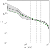
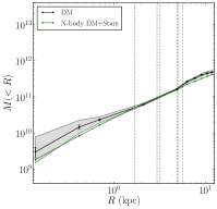
We generate four two-component mock galaxies, where the dark matter and stellar profiles are allowed to be both steep and shallow. The enclosed mass of the stars and dark matter are both fixed to be M⊙ at the stellar scale radius kpc, such that the stars and dark matter contribute equally to the total mass at . The dark matter scale length is fixed for all models at kpc. These values were chosen to closely resemble the lensing galaxy PG1115+080 (Weymann et al., 1980). We place the galaxy at a redshift of for lensing. Throughout, we assume a cosmology where Gyr, , and . The critical lensing density is /kpc2.
The galaxies were generated as three dimensional particle distributions as in Dehnen (2009). Each component follows the profile:
| (18) |
where is the component scale radius mentioned in Table 1; is the ellipsoidal radius; and the axis ratios are . In the case where the central density profile index is unity (and in the limit of spherical symmetry), this is the Hernquist profile (Hernquist, 1990). The four combinations of profile indices are shown in Table 1.
| Galaxy | |||||
|---|---|---|---|---|---|
| star1.0-dmCore | 1 | 4 | 0.05 | 50 kpc | |
| star1.0-dmCusp | 1 | 4 | 1 | 50 kpc | |
| star1.5-dmCore | 1.5 | 0.16 | 50 kpc | ||
| star1.5-dmCusp | 1.5 | 1 | 10 kpc |
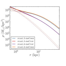

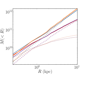
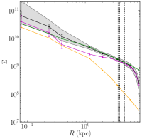
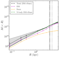
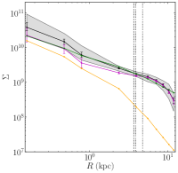
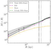
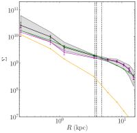
In Figure 1, we show the 3D radial density, the 2D projected density, and the 2D enclosed mass for each galaxy.
4.2 Lens configurations
For each of the four galaxies, we used the raytracing feature of Glass described in §3.5 to construct 6 basic lensing morphologies:
-
1.
one double and one extended double;
-
2.
one quad and one extended quad;
-
3.
two 2-source quads with varying redshift contrast.
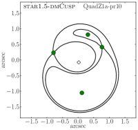
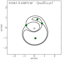
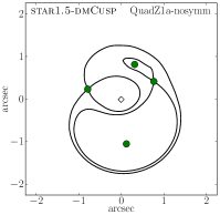
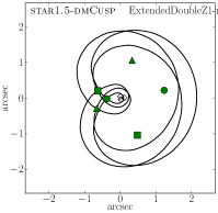
The ‘extended’ configurations use multiple point sources at the same redshift to simulate an extended source that will produces an arc-like image. Figure 2 shows the lens configurations for the star1.5-dmCusp galaxy. The configurations for the other galaxies are similar. The labels Z1, Z2, Z3 within the names refer to the redshift of the sources. We have chosen Z1=1.72, Z2=0.72, and Z3=0.51 so that the radial distribution of the images is roughly equally spaced. For all mocks, we do not apply any external shear field. Only the central image of the Z1 source is used to avoid over-constraining the models, otherwise all the central images would fall within the central pixel and no solution exists that satisfies all locations simultaneously for one pixel value.
Each of these configurations were modelled with and without time delays; with and without a central image; and with and without the stellar mass as a lower bound, for a total of 48 test cases. (The central image is typically highly demagnified. For galaxy lenses it is very difficult to find since it lies along the sight line to the bright lensing galaxy; in clusters, however, such images have been seen – e.g., Inada et al. 2005). We assumed for all our tests that the lensing mass was radially symmetric (Prior vi). For our mock data, this is known to be true; it is most often the case with real galaxies, unless there is an obvious observed asymmetry. (We explore the effect of switching off the symmetry prior in Appendix C. For the quads, the difference is small; for the doubles – as expected – the results are significantly degraded without this prior.) We use, by default, 8 pixels from the centre to the edge of the mass map; the central pixel was further refined into pixels to capture any steep rise in the profile (two of the four mock galaxies have a steeply rising inner profile). We demonstrate that our results are robust to changing the grid resolution in Appendix D.
In all cases – despite applying no external shear to the mock lenses – we allow a broad range of external shear in our lens model reconstructions. Glass correctly returns a small or zero shear in all cases. It is possible that more complex shear fields present in real lensing galaxies could introduce further degeneracies beyond those discussed here. However, any such shear field can, at least in principle, be constrained by data (e.g., combining weak lensing constraints, or assuming that the shear field correlates with visible galaxies – e.g., Merten et al. 2009; Wong et al. 2011).
5 Results
5.1 Radial profile recovery
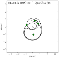
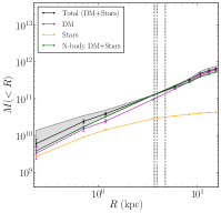
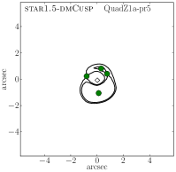
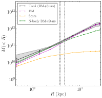
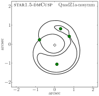
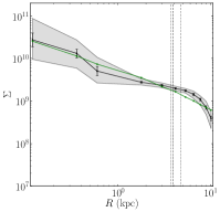
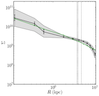
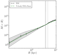
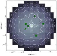
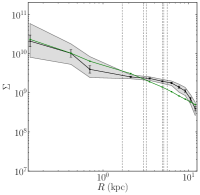
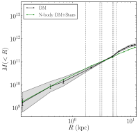
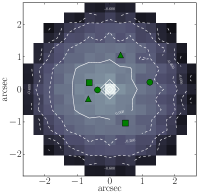
Figure 3 shows some example reconstructions of the radial profile of our mock lenses. The left column shows the ensemble average arrival time surface with images marked as circles and the inferred source positions as diamonds. The centre column shows the radial density profile. The error bars cover a range around the median; the grey bands show the full ensemble range. The true density profile from the mock data is also plotted for comparison. The vertical lines mark the radial position of the images. The right column shows the enclosed mass. From top to bottom, the rows correspond to an extended double for star1.5-dmCusp; an extended double with stellar mass constraints for star1.5-dmCusp; a quad with time delay data for star1.5-dmCusp; and a quad with time delays for star1.0-dmCore. Figure 5 shows an example 2D reconstruction for star1.5-dmCusp for a quad; we discuss shape recovery further in §5.2.
As expected, the accuracies and precisions are best in the range of radii with lensed images where the most information about the lens is present. Even in the weakly constrained case of the extended double where the radial profile is poor, the true enclosed mass is well recovered at the image radii and our ensemble always encompasses it. We have verified this is the case in all of our tests, although for brevity we have not included the plots here. In all cases, there is a dip in the profile at large due to the cut off in mass in the lensing map. This is of little importance, though, as there is no lensing information there.
Notice that the extended double (top row) gives the poorest constraints, as expected. Adding stellar mass (second row) significantly improves the constraints, for this example where the stars contribute significantly to the potential. Moving to a quad with time delays gives constraints almost as strong as the double with stellar mass, but note that focussing only on the goodness of the fit can be misleading. In the third row of Figure 3, we obtain a better recovery than in the bottom row for precisely the same data quality. This occurs because the Glass prior favours steeper models consistent with star1.5-dmCusp, but not star1.0-dmCore. It is the Glass prior, rather than the data that is driving the good recovery for star1.5-dmCusp in this example. This emphasises the importance of using a wide range of mock data tests to determine the role of data versus prior in strong lensing.
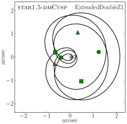
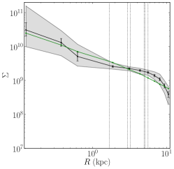
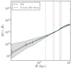
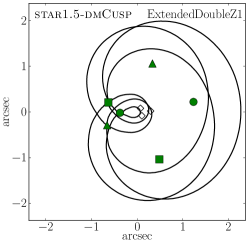
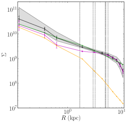
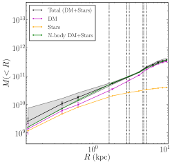
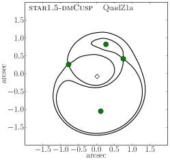
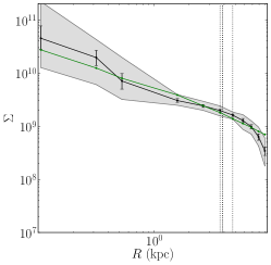
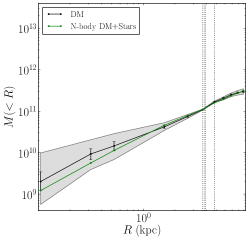
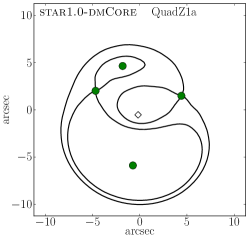
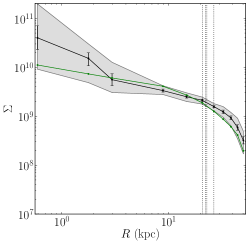
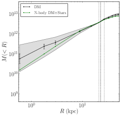
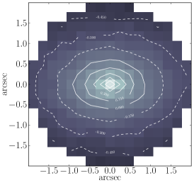
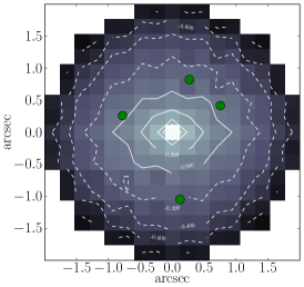
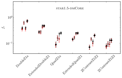
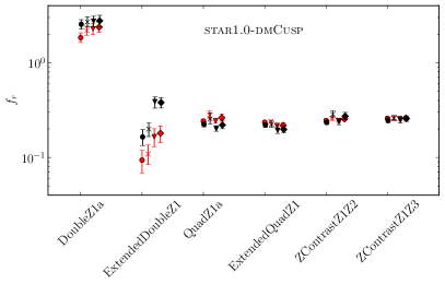
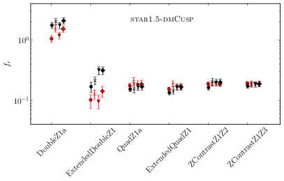
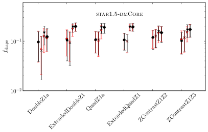
Figure 6 and Figure 7 show the results for our full mock data ensemble. Each subplot corresponds to a different mock galaxy, as marked. We show the fractional error of the mass distribution for each of the test configurations with (red) and without (black) stellar mass. In Figure 6 we define the error:
| (19) |
based on the mass of each pixel ring and the mass from the mock galaxy. In Figure 7 the error is defined over all the pixels :
| (20) |
Since both error measurements consider the mass of each pixel, we are implicitly weighting the recovered density by the varying size of the pixels. The value emphasises the error one would see from radial profiles, while is useful as a measure of how well each individual pixel is recovered. For both and , we only consider mass up to one pixel length passed the outermost image, since there is no longer any lensing information beyond that point. This means we typically use 8 bins, linearly spaced, ignoring the outermost 3 bins. The spacing changes, however, at the border between the high resolution region in the middle.
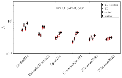
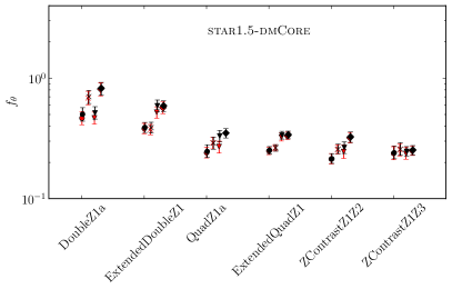
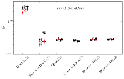
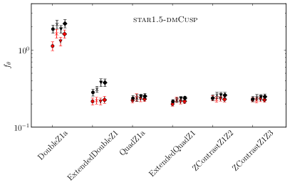
The abundance of strong lensing data increases from left to right within each plot. As a result, there is a general trend for the reconstruction quality to increase (and therefore for to decrease). When both time delays and a central image are present (TD+central), the quality is highest. A double is known to provide very little constraint on the mass distribution. This is particularly evident in galaxies star1.0-dmCusp and star1.5-dmCusp where the mass profile is steepest and the reconstruction of the double is poorest. However, the addition of an arc from the extended source is sufficient to correct this. Notice that, as in Figure 3, the recovery for star1.5-dmCusp quickly saturates; there is little improvement as the data improves beyond a single quad. This occurs because the Glass sample prior in the absence of data favours steep models like star1.5-dmCusp over shallower models like star1.0-dmCore (see also Figure 3).
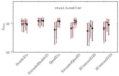
5.2 Shape recovery
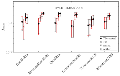
Figure 7 already gives us important information about how well we can recover the shape of a lens. The trends are very similar to the radial profile recovery in Figure 6, suggesting that if the radial profile is well-recovered then, typically, the shape is too. A notable exception is for the star1.5-dmCusp models where adding stellar mass constraints aids the shape recovery, but little-improves the radial mass profile. A visual example of the shape recovery is given in Figure 5.
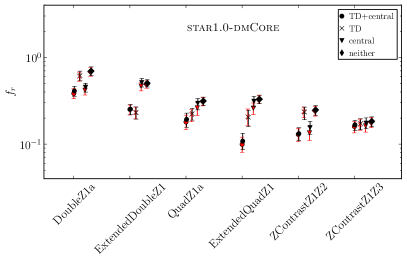
We can also more directly probe the recovery of the shape of the mass distribution by considering the ratio of the major and minor axes of the inertia ellipse. If they are equal, the mass is distributed uniformly on the projected disc. The more dissimilar they are, the more elliptical the mass distribution. We define the global measure of lens shape as:
| (21) |
where and are the eigenvalues of the 2D inertia tensor:
| (22) |
We always take to be the largest value. As with and , we only consider mass up to one radial position passed the outermost image and compute the fractional error as:
| (23) |
where is the shape of the mock galaxy. The distribution of for each mock galaxy and each test case is shown in Figure 8. Interestingly, for this global shape parameter recovery it appears more important to have time delay data and/or a central image (TD,TD+central) than to have a quad or multiple sources with wide redshift separation. In all cases, the stellar mass little-aids the recovery, reflecting the fact that is heavily weighted towards the shape at the edge of the mass map, rather than at the centre where the stars may dominate the potential (see Eq. (22)).

5.3 Stellar mass
The stellar mass distribution gives a lower bound on the total mass. Where the stars dominate the central potential, it can provide a powerful constraint extra to the strong lensing data. We took the stellar mass directly from the generated galaxies and projected the particles onto the pixels. Glass also offers an option to interpolate any map of stellar mass (e.g., from an observation) onto the pixels. The linear constraint is added to Glass by writing as the sum of the dark matter and stellar mass components in the potential (Eq. 14). Since each is just a constant we do not add new, separate equations for each pixel. Although we assume a perfect recovery of the stellar mass with no error on the lower mass bound, it is straightforward to add errors as the stellar mass constraint remains linear: , where is an additional error parameter.
With the stellar mass lower bound, there is a significant improvement of the reconstruction quality shown in Figure 6 and Figure 7 for the doubles in the steepest mock galaxies (star1.0-dmCusp and star1.5-dmCusp). This is because these models are dominated by stars in the inner region. By contrast, the other two galaxies – where the stars contribute negligibly to the potential – are largely unaffected.
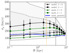
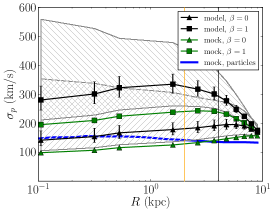
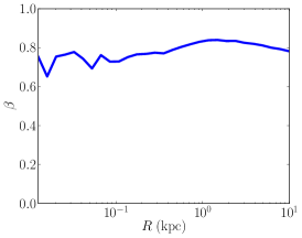
5.4 Stellar kinematics
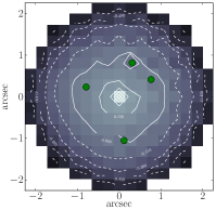
As outlined in §3, Glass can also run post processing routines on the model ensemble which can be used to apply non-linear constraints. As an example, we consider here constraints from stellar kinematics. The models in the Glass ensemble are processed as described in §3.7. To illustrate the power of stellar kinematic constraints, in Figure 9, we plot the projected velocity dispersion calculated for one model model (extracted from the full ensemble) of the star1.5-dmCusp Quad with time delays and no stellar mass (left), and the same but with stellar mass (middle). In both cases, we calculate curves for two extrema velocity anisotropies: (green) and (red). Over-plotted is the correct answer for the star1.5-dmCusp model (black). The stellar half mass radius (yellow) Einstein radius (black) are marked by vertical lines. For this configuration, these two radii are well-separated.
Without even sweeping through the model ensemble and formally accepting/rejecting models, Figure 9 already illustrates what we can obtain from stellar kinematics. The left plot shows the radially averaged projected velocity dispersion (Eq. 12) for a single quad from the star1.5-dmCusp galaxy without the stellar mass constraint. The blue data points show the 1 distribution from the ensemble assuming (solid) and (dashed); the grey bands show the full distributions. Also marked are the calculated from the mock data assuming (solid purple) and (dashed purple); and the true measured directly from the stars (black). This latter has a non-constant (right panel) and differs also from the purple and blue curves in that these all assume spherical symmetry, whereas the stellar distribution is really triaxial. Such triaxiality and varying explains why the purple curves do not match the black one. However, they do largely bracket the correct solution. More interestingly, the curves approximately cross for at the stellar half light radius (yellow vertical line). This demonstrates, as has previously been reported in the literature, that gives a good estimate of the mass enclosed within the half light radius (e.g., Walker et al., 2009; Wolf et al., 2010). The mass profile, however, depends on which is poorly constrained by these data. If we add stellar mass constraints (middle panel), the situation is little-improved. The true answer already lay close to the bottom of the ensemble distribution; it now is forced to lie right at the edge.
From Figure 9, it is clear that provides two useful pieces of information. Firstly, it is a powerful probe of . Given a measurement of km/s, we could usefully reject many models in the ensemble as being overly steep in the centre. We would not, however, obtain a strong constraint on . We could rule out (blue dashed line), but since our model crosses the true line at it is clear that many profiles will be consistent with the data. On the other hand, if we have a situation where (i.e. the vertical yellow and black lines in Figure 9 overlap), then we will obtain tight constraints on since we then have two strong constraints on that become redundant. This latter situation of redundancy is also exactly what we would like to constrain cosmological parameters. In this case, we require a third piece of redundant information – in this case in the form of strong lensing time delays. We will discuss such cosmological constraints in a forthcoming paper.
The results for stellar kinematics match our expectations from §2.3. Where the lens data already constrain the mass distribution at , stellar kinematics provide valuable information about the velocity anisotropy of the stars, (see Figure 9). Where the lens data poorly constrain the mass distribution at , we may ‘integrate out’ the effect of unknown to obtain a robust measure of from the stellar kinematics. This latter is robust to both uncertainties in and to our assumption of spherical symmetry in the kinematic models (Agnello & Evans, 2012).
6 Conclusions
We have introduced a new gravitational lens modelling tool – Glass – and used it to test the recovery of the mass profile and shape of mock strong lensing galaxies. Our key findings are as follows:
-
1.
For pure lens data, multiple sources with wide redshift separation give the strongest constraints as this breaks the well-known mass-sheet or steepness degeneracy;
-
2.
A single quad with time delays also performs well, giving a good recovery of both the mass profile and its shape;
-
3.
Stellar masses – for lenses where the stars dominate the central potential – can also break the steepness degeneracy, giving a recovery for doubles almost as good as having a quad with time delay data, or multiple source redshifts;
-
4.
If the radial density profile is well-recovered, so too is the shape of a lens;
-
5.
Stellar kinematics provide a robust measure of the mass at the half light radius of the stars that can also break the steepness degeneracy if – the Einstein radius; and
-
6.
If , then stellar kinematic data can be used to probe the stellar velocity anisotropy – an interesting quantity in its own right.
Where information on the mass distribution from lensing and/or other probes becomes redundant, this opens up the possibility of using strong lensing to constrain cosmological models. We will study this, and present the first results from Glass applied to real data, in forthcoming papers.
7 Acknowledgments
The authors would like to thank Sarah Bryan and Walter Dehnen for creating the particle distributions for the mock galaxies, and the anonymous referee for many useful suggestions which has improved the manuscript. JIR would like to acknowledge support from SNF grant PP00P2_128540/1.
References
- AbdelSalam et al. (1998) AbdelSalam H. M., Saha P., Williams L. L. R., 1998, AJ, 116, 1541
- Agnello & Evans (2012) Agnello A., Evans N. W., 2012, ApJ, 754, L39
- Amendola et al. (2013) Amendola L. et al., 2013, Living Reviews in Relativity, 16, 6
- Barnabè et al. (2011) Barnabè M., Czoske O., Koopmans L. V. E., Treu T., Bolton A. S., 2011, MNRAS, 415, 2215
- Barnabè et al. (2009) Barnabè M., Nipoti C., Koopmans L. V. E., Vegetti S., Ciotti L., 2009, MNRAS, 393, 1114
- Bartelmann (2010) Bartelmann M., 2010, Classical and Quantum Gravity, 27, 233001
- Bernstein & Fischer (1999) Bernstein G., Fischer P., 1999, AJ, 118, 14
- Binney & Tremaine (2008) Binney J., Tremaine S., 2008, Galactic Dynamics: Second Edition. Princeton University Press
- Blandford & Narayan (1986) Blandford R., Narayan R., 1986, ApJ, 310, 568
- Bolton et al. (2008) Bolton A. S., Burles S., Koopmans L. V. E., Treu T., Gavazzi R., Moustakas L. A., Wayth R., Schlegel D. J., 2008, ApJ, 682, 964
- Broadhurst & Barkana (2008) Broadhurst T. J., Barkana R., 2008, MNRAS, 390, 1647
- Bruzual & Charlot (2003) Bruzual G., Charlot S., 2003, MNRAS, 344, 1000
- Cenarro et al. (2004) Cenarro A. J., Sánchez-Blázquez P., Cardiel N., Gorgas J., 2004, ApJ, 614, L101
- Chabrier (2003) Chabrier G., 2003, PASP, 115, 763
- Coe et al. (2010) Coe D., Benítez N., Broadhurst T., Moustakas L. A., 2010, ApJ, 723, 1678
- Coe et al. (2014) Coe D., Bradley L., Zitrin A., 2014, ArXiv e-prints
- Coles (2008) Coles J., 2008, ApJ, 679, 17
- Collett et al. (2012) Collett T. E., Auger M. W., Belokurov V., Marshall P. J., Hall A. C., 2012, MNRAS, 424, 2864
- Conroy & van Dokkum (2012) Conroy C., van Dokkum P., 2012, ApJ, 747, 69
- Dehnen (2009) Dehnen W., 2009, MNRAS, 395, 1079
- Diego et al. (2005) Diego J. M., Protopapas P., Sandvik H. B., Tegmark M., 2005, MNRAS, 360, 477
- Dutton et al. (2013) Dutton A. A. et al., 2013, MNRAS, 428, 3183
- Falco et al. (1985) Falco E. E., Gorenstein M. V., Shapiro I. I., 1985, ApJ, 289, L1
- Ferreras et al. (2013) Ferreras I., La Barbera F., de la Rosa I. G., Vazdekis A., de Carvalho R. R., Falcón-Barroso J., Ricciardelli E., 2013, MNRAS, 429, L15
- Ferreras et al. (2008) Ferreras I., Saha P., Burles S., 2008, MNRAS, 383, 857
- Ferreras et al. (2010) Ferreras I., Saha P., Leier D., Courbin F., Falco E. E., 2010, MNRAS, 409, L30
- Ferreras et al. (2005) Ferreras I., Saha P., Williams L. L. R., 2005, ApJ, 623, L5
- Hernquist (1990) Hernquist L., 1990, ApJ, 356, 359
- Inada et al. (2005) Inada N. et al., 2005, PASJ, 57, L7
- Johnson et al. (2014) Johnson T. L., Sharon K., Bayliss M. B., Gladders M. D., Coe D., Ebeling H., 2014, ArXiv e-prints
- Jullo et al. (2010) Jullo E., Natarajan P., Kneib J.-P., D’Aloisio A., Limousin M., Richard J., Schimd C., 2010, Science, 329, 924
- Keeton (2010) Keeton C. R., 2010, General Relativity and Gravitation, 42, 2151
- Keeton et al. (1998) Keeton C. R., Kochanek C. S., Falco E. E., 1998, ApJ, 509, 561
- Kneib & Natarajan (2011) Kneib J.-P., Natarajan P., 2011, A&A Rev., 19, 47
- Kochanek (2002a) Kochanek C. S., 2002a, ArXiv Astrophysics e-prints
- Kochanek (2002b) Kochanek C. S., 2002b, ApJ, 578, 25
- Kochanek et al. (2000) Kochanek C. S. et al., 2000, ApJ, 543, 131
- Koopmans et al. (2006) Koopmans L. V. E., Treu T., Bolton A. S., Burles S., Moustakas L. A., 2006, ApJ, 649, 599
- Leier et al. (2011) Leier D., Ferreras I., Saha P., Falco E. E., 2011, ApJ, 740, 97
- Liesenborgs et al. (2006) Liesenborgs J., De Rijcke S., Dejonghe H., 2006, MNRAS, 367, 1209
- Liesenborgs et al. (2007) Liesenborgs J., de Rijcke S., Dejonghe H., Bekaert P., 2007, MNRAS, 380, 1729
- Liesenborgs et al. (2008) Liesenborgs J., de Rijcke S., Dejonghe H., Bekaert P., 2008, MNRAS, 386, 307
- Lubini & Coles (2012) Lubini M., Coles J., 2012, MNRAS, 425, 3077
- Lubini et al. (2014) Lubini M., Sereno M., Coles J., Jetzer P., Saha P., 2014, MNRAS, 437, 2461
- Merten et al. (2009) Merten J., Cacciato M., Meneghetti M., Mignone C., Bartelmann M., 2009, A&A, 500, 681
- Newman et al. (2013) Newman A. B., Treu T., Ellis R. S., Sand D. J., 2013, ApJ, 765, 25
- Paraficz & Hjorth (2010) Paraficz D., Hjorth J., 2010, ApJ, 712, 1378
- Pontzen et al. (2013) Pontzen A., Roškar R., Stinson G. S., Woods R., Reed D. M., Coles J., Quinn T. R., 2013, pynbody: Astrophysics Simulation Analysis for Python. Astrophysics Source Code Library, ascl:1305.002
- Read et al. (2007) Read J. I., Saha P., Macciò A. V., 2007, ApJ, 667, 645
- Refsdal (1964) Refsdal S., 1964, MNRAS, 128, 307
- Refsdal (1966) Refsdal S., 1966, MNRAS, 132, 101
- Richard et al. (2014) Richard J. et al., 2014, MNRAS, 444, 268
- Rusin et al. (2003) Rusin D. et al., 2003, ApJ, 587, 143
- Saha (2000) Saha P., 2000, AJ, 120, 1654
- Saha & Read (2009) Saha P., Read J. I., 2009, ApJ, 690, 154
- Saha et al. (2006) Saha P., Read J. I., Williams L. L. R., 2006, ApJ, 652, L5
- Saha & Williams (1997) Saha P., Williams L. L. R., 1997, MNRAS, 292, 148
- Saha & Williams (2004) Saha P., Williams L. L. R., 2004, AJ, 127, 2604
- Saha & Williams (2006) Saha P., Williams L. L. R., 2006, ApJ, 653, 936
- Saha et al. (2007) Saha P., Williams L. L. R., Ferreras I., 2007, ApJ, 663, 29
- Schneider (2014) Schneider P., 2014, A&A, 568, L2
- Schneider & Sluse (2014) Schneider P., Sluse D., 2014, A&A, 564, A103
- Sendra et al. (2014) Sendra I., Diego J. M., Broadhurst T., Lazkoz R., 2014, MNRAS, 437, 2642
- Sereno & Paraficz (2014) Sereno M., Paraficz D., 2014, MNRAS, 437, 600
- Suyu et al. (2014) Suyu S. H. et al., 2014, ApJ, 788, L35
- Treu & Koopmans (2002) Treu T., Koopmans L. V. E., 2002, MNRAS, 337, L6
- Vegetti et al. (2010) Vegetti S., Koopmans L. V. E., Bolton A., Treu T., Gavazzi R., 2010, MNRAS, 408, 1969
- Walker et al. (2009) Walker M. G., Mateo M., Olszewski E. W., Peñarrubia J., Wyn Evans N., Gilmore G., 2009, ApJ, 704, 1274
- Walsh et al. (1979) Walsh D., Carswell R. F., Weymann R. J., 1979, Nature, 279, 381
- Weymann et al. (1980) Weymann R. J. et al., 1980, Nature, 285, 641
- Wilkinson et al. (2002) Wilkinson M. I., Kleyna J., Evans N. W., Gilmore G., 2002, MNRAS, 330, 778
- Williams & Saha (2000) Williams L. L. R., Saha P., 2000, AJ, 119, 439
- Wolf et al. (2010) Wolf J., Martinez G. D., Bullock J. S., Kaplinghat M., Geha M., Muñoz R. R., Simon J. D., Avedo F. F., 2010, MNRAS, 406, 1220
- Wong et al. (2011) Wong K. C., Keeton C. R., Williams K. A., Momcheva I. G., Zabludoff A. I., 2011, ApJ, 726, 84
- Young et al. (1981) Young P., Gunn J. E., Oke J. B., Westphal J. A., Kristian J., 1981, ApJ, 244, 736
- Zwicky (1937) Zwicky F., 1937, ApJ, 86, 217
Appendix A Implementation Details
Since we want to model the density distribution with a computer it is convenient to choose units that make the relevant quantities of order unity. We therefore measure lengths in light years, time in years, positions in arcseconds, and choose and , where arcsec/rad. The mass unit is then . It will also be useful to define a proxy to the Hubble constant . We now express the equations from §2 in terms of these new units and introduce some other useful quantities.
The lens equation in its complete form becomes:
| (24) | |||||
where the factor of in the second term comes from the fact that has units of /lyr2. We can clean this up by first writing down a dimensionless time delay
| (25) |
in terms of our previous definitions and defining . We further define a dimensionless density
| (26) |
and a lensing potential
| (27) |
Now we can express Eq. (24) very compactly as
| (28) |
where . We explicitly write to remind ourselves that there is no source distance factor involved. This is useful when we consider multiple sources.
Appendix B Derivation of pixelated density coefficients
When the lens plane is pixelized we need a discrete form of the integral
In particular we want
where is the logarithm evaluated over the th pixel at position . Let the pixel side length be . Instead of working with a position vector we work in Cartesian coordinates where . The integral now becomes
where and similarly for . Using the identity
we can express as the sum of four parts
where
Appendix C No radial symmetry prior
In this appendix, we explore the effect of the radial symmetry prior. Figure 10 shows results for a single quad (top two rows) and an extended double (bottom two rows) without the radial prior; in both cases, we do not use the stellar mass constraints. The bottom row of each group uses time delay data. Without time delay data or the radial symmetry prior, the results for the quad are poor – particularly the shape recovery. Including time delays, the results are similar to the case with the radial prior (Figure 3 and Figure 5). Similarly, for the extended double the results without time delays are poor. Even with time delays, the shape is not well recovered without the radial prior, as expected.


Appendix D Pixel resolution convergence test
In this Appendix, we present a convergence test of our results with the grid resolution – . By default, this is set to 8 pixels from the centre of the mass map to the edge. As can be seen from Figure 11, our results are typically well-converged for . The results for become systematically biased away from the central regions (where we have the higher resolution adaptive mesh), because our regularisation prior combined with a low biases us towards shallow models. This effect diminishes with increasing resolution and is already negligible by . Notice that the mass increases in size with decreasing resolution. This is because we always demand that there are four pixels beyond the outermost image.