Type Ia Supernova Rate Measurements to Redshift 2.5 from CANDELS:Searching for Prompt Explosions in the Early Universe

Abstract

The Cosmic Assembly Near-infrared Deep Extragalactic Legacy Survey (CANDELS) was a multi-cycle treasury program on the Hubble Space Telescope (HST) that surveyed a total area of $\sim$0.25 deg² with $\sim$900 HST orbits spread across 5 fields over 3 years. Within these survey images we discovered 65 supernovae (SN) of all types, out to $z\approx 2.5$. We classify $\sim$24 of these as Type Ia SN (SN Ia) based on host-galaxy redshifts and SN photometry (supplemented by grism spectroscopy of 6 SN). Here we present a measurement of the volumetric SN Ia rate as a function of redshift, reaching for the first time beyond $z=2$ and putting new constraints on SN Ia progenitor models. Our highest redshift bin includes detections of SN that exploded when the universe was only $\sim$3 Gyr old and near the peak of the cosmic star-formation history. This gives the CANDELS high-redshift sample unique leverage for evaluating the fraction of SN Ia that explode promptly after formation ($<$500 Myr). Combining the CANDELS rates with all available SN Ia rate measurements in the literature we find that this prompt SN Ia fraction is $f_{P}$=0.53 $\begin{subarray}{c}\pm\\ \mbox{\scalebox{0.45}{stat}}\end{subarray}$${}^{0.09}_{0.10}$ $\begin{subarray}{c}\pm\\ \mbox{\scalebox{0.45}{sys}}\end{subarray}$${}^{0.10}_{0.26}$, consistent with a delay time distribution that follows a simple $t^{-1}$ power law for all times $t>40$ Myr. However, a mild tension is apparent between ground-based low-$z$ surveys and space-based high-$z$ surveys. In both CANDELS and the sister HST program CLASH, we find a low rate of SN Ia at $z>1$. This could be a hint that prompt progenitors are in fact relatively rare, accounting for only $\sim$20% of all SN Ia explosions – though further analysis and larger samples will be needed to examine that suggestion.

I. Introduction

The prevailing model for a Type Ia supernova (SN Ia) progenitor system begins with a binary system in which the primary star evolves to become a white dwarf (WD). The WD acquires mass from its companion star, approaches the Chandrasekhar limit, and explodes in a thermonuclear runaway (for reviews, see Hillebrandt & Niemeyer 2000; Livio 2001). The companion star that feeds the WD and thereby sets off the thermonuclear bomb is one of the key components of this model, but remains a topic of ongoing debate. In single-degenerate (SD) models, the companion is a main sequence or evolved giant star, transferring mass via Roche-lobe overflow, stellar winds or other means (Whelan & Iben 1973). In double-degenerate (DD) models the companion is another WD, merging with the primary after a period of orbital decay driven by gravitational wave radiation (Iben & Tutukov 1984; Webbink 1984). More recent variations on these pathways to explosion include the “core-degenerate scenario” (Kashi & Soker 2011) and perturbation-induced mergers in triple systems (Thompson 2011).

The SN Ia explosion rate as a function of redshift, SNR($z$), can provide an important observational test to constrain SN Ia progenitor models and possibly distinguish between them. In this paper we will present measurements of the SN Ia rate as a function of redshift and use them to place new constraints on SN Ia progenitor models, particularly on the fraction of SN Ia progenitors that explode within 500 Myr after their formation.

Suppose we have a burst of star formation in a galaxy, such that the star-formation rate can be approximated by a delta function in time. Binary population synthesis modeling gives us the initial conditions of all the binaries (mass, orbital separation, etc.), and a progenitor model sets the conditions necessary for explosion as a SN Ia. Using a stellar evolution model, one can follow the binary systems as they evolve, measuring the delay time distribution (DTD) between formation and explosion. To put constraints on SNIa progenitor models, we can translate this DTD to cosmic scales and compare it to the observed volumetric SN Ia rate as a function of look-back time, as first proposed by Madau et al. (1998).

Volumetric SN Ia rates before completion of the CANDELS and CLASH SN surveys. Assorted ground-based surveys are plotted as white circles (Blanc et al. 2004; Botticella et al. 2008; Cappellaro et al. 1999; Dilday et al. 2010; Hardin et al. 2000; Horesh et al. 2008; Graur & Maoz 2013; Li et al. 2011; Melinder et al. 2012; Pain et al. 2002; Perrett et al. 2012; Rodney & Tonry 2010; Tonry et al. 2003). Three high-redshift SN surveys are highlighted: gray circles for the Subaru Deep Field (SDF, Graur et al. 2011), blue downward triangles for volumetric (not cluster) rates from the Cluster Supernova Survey (CSS, Barbary et al. 2012), green upward triangles for the GOODS and PANS surveys (Dahlen et al. 2008).

As shown in Figure I, recent measurements of the SN Ia rate at low redshift ($z<1$) are in good agreement, consistently finding that the SNR($z$) rises steadily to at least $z\approx 1$ (e.g., Rodney & Tonry 2010; Dilday et al. 2010; Perrett et al. 2012). However, at $z>1$ the trend of the SNR($z$) curve is much less clear. The spectral energy distribution of a SN Ia peaks in the rest-frame B band with an absolute magnitude around -19.5. At $z=1.2$ that peak brightness becomes fainter than 25th magnitude in the observer’s $z$ band – making discovery and light curve follow-up nearly impossible for ground based observatories.

For that reason, space-based surveys using the Hubble Space Telescope’s Advanced Camera for Surveys (ACS) have been the primary vehicle for tracking the SNR($z$) to $z\approx 1.5$. The GOODS+PANS surveys were the first programs to extend rate measurements beyond $z\approx 1$ (Dahlen et al. 2004, 2008), and their measured rates suggested a peak in the SN Ia rate at $z\approx 1.2$, with a decline at higher redshifts. Independent examination of the same survey data recovered the same trend (Kuznetsova et al. 2008), although both analyses were limited by a small sample size in the highest redshift bin. Subsequently, the Cluster Supernova Survey (CSS) of the Supernova Cosmology Project used ACS to measure the volumetric SN Ia rate (Barbary et al. 2012). These data revealed a similar peak and decline, although with even larger uncertainty in the high-$z$ bins. From the ground, the Subaru Deep Field (SDF) SN survey used the Suprime-cam imager on the Subaru telescope to reach similar redshifts (Poznanski et al. 2007; Graur et al. 2011). As can be seen in Figure I, these SDF rates formally show no decline in the highest redshift bin, but they are consistent with the ACS results, within the errors.

The ACS high-$z$ SN Ia generally have reliable classifications, based on well-sampled multi-band light curves, spectroscopic redshifts, and HST grism spectroscopy of most SN Ia candidates. However, due to the relatively small survey area, these programs have very large statistical uncertainties (Dahlen et al. (2008) have $\sim$3 SN in their highest redshift bin, Barbary et al. (2012) have $\sim$1). In contrast, the SDF survey built up a larger sample (10 SN Ia at $z\approx 1.5$) but their survey design introduced a potential for large systematic biases. The SDF epochs were spaced by $\sim$1 year, meaning that the phase of the SN light curve at discovery was unconstrained, and the classification of detected SN was based on only a single epoch of photometric data in the R,i$\prime$,z$\prime$ bands. Furthermore, redshifts for the SDF high-$z$ SN sample were based almost exclusively on photometric redshift estimates of the SN host galaxies, not as precise or reliable as spectroscopic redshifts $-$ though see Frederiksen:2012b for one spectroscopic confirmation of a SDF host galaxy at $z=1.55$.

An apparent peak in the SN Ia rate at $z\approx 1$ and a decline toward $z=1.5$ has been interpreted as indicating a delay of $>1$ Gyr between formation and explosion for most SN Ia (Strolger et al. 2004, 2010). This would be broadly consistent with some SD models, and inconsistent with DD models, which typically predict a large fraction of SN Ia that explode promptly after star formation (within 1 Gyr). A clear measurement of the shape of the SN Ia rate function at $z>1$ would provide an important constraint on DTD models, and would go a long way toward resolving the question of whether a SD or DD model could be the dominant progenitor channel for all SN Ia at all redshifts. Given the problems with current high-$z$ SN rates, there is a clear need to improve the measurement by expanding the sample of well-classified SN at $z>1$.

In this paper we present a measurement of the SNR($z$) from a sample of 65 SN discovered in the CANDELS SN program, extending the SNR($z$) measurement for the first time to $z=2.5$. This SN survey is a joint operation of two HST Multi-Cycle Treasury (MCT) programs: the Cosmic Assembly Near-infrared Deep Extragalactic Legacy Survey (CANDELS; PIs:Faber and Ferguson; Grogin et al. 2011; Koekemoer et al. 2011), and the Cluster Lensing and Supernovae search with Hubble (CLASH; PI:Postman; Postman et al. 2012). The SN discovery and follow-up for both programs were allocated to the HST MCT SN program (PI:Riess). The results presented here are based on the full five fields and $\sim$0.25 deg² of the CANDELS program, observed from 2010 to 2013. A companion paper presents the SN Ia rates from the CLASH sample (Graur et al. 2014). A composite analysis that combines the CANDELS+CLASH SN sample and revisits past HST surveys will be presented in a future paper.

In Section II we describe the SN search component of the CANDELS survey, and in Section III we describe our detection efficiency measurements. Our photometric SN classifications are presented in Section IV, properties of the SN host galaxies are described in Section V, and in Section VI we detail new grism spectroscopy for 4 of our SN. The rates calculation is described in Section VII and we discuss the consequences for SN Ia progenitor models in Section VIII. Finally, a summary is presented in Section IX. In tables and figures throughout the paper, we present the subset of 14 SN with $z>1.5$ in the main body of the text, with the remaining 51 shown in Appendix B. Throughout this work we assume a flat $\Lambda$CDM cosmology with $H_{0}$=70, $\Omega_{\rm m}$=0.3 and $\Omega_{\Lambda}$=0.7.

II. The CANDELS SN Survey

The 3-year CANDELS program was designed to probe galaxy evolution out to $z\approx 8$ with deep infrared (IR) and optical imaging of five well-studied extragalactic fields: GOODS-S, GOODS-N, COSMOS, UDS, and EGS. As described fully in Grogin et al. (2011), the CANDELS program includes both “wide” and “deep” fields. The wide component of CANDELS comprises the COSMOS, UDS, and EGS fields, plus one third of the GOODS-S field and one half of the GOODS-N field – a total survey area of 730 square arcminutes. The CANDELS survey provides two visits to each wide field, spaced by $\sim$50 days. The “deep” component of CANDELS came from the central 67 square arcminutes of each of the GOODS-S and GOODS-N fields. These deep regions were each visited 15 times over the course of two years (2010-2012 for GOODS-S, 2012-2013 for GOODS-N). Only 10 of those visits are used for SN discovery (the other visits lack template data for generating difference images), and those 10 epochs are also spaced at a cadence of $\sim$50 days. The CANDELS fields analyzed in this work are described in Table 1.

Table 2 presents the exposure times and 5$\sigma$ limiting magnitudes for a typical single-epoch set of exposures. Each CANDELS visit includes a set of four IR exposures from the Wide Field Camera 3 (WFC3) IR detector: two in F160W ($H$ band) and two in F125W ($J$ band). These are the search filters for the CANDELS SN survey (i.e., all SN in our sample are IR detections). Additionally, each observation set includes a broad optical band, which helps to distinguish SN Ia from core-collapse supernovae (CC SN) and other transients (see Section IV). In $\sim$80% of the SN search visits, this blue component is collected within minutes of the IR exposures as a single exposure using the WFC3 UVIS camera in the F350LP filter (a broad “white light” filter that we refer to as “W band”). In the remaining $\sim$20% of visits (in the wide fields) the W band exposure is replaced with ACS observations in the F606W filter (broad V band), and complemented by the ACS F814W filter (broad I band). These ACS observations come from coordinated parallel visits and are taken within 3 days of the primary IR visit.

Table 1CANDELS SN Survey Fields

	R.A.	Decl	WFC3-IR	Searchable Area	SN Search
Field	(J2000)	(J2000)	Tiles/Epoch	(arcmin2)	Epochs (MJD)
COSMOS	10:00:28	$+$02:12:04	44	196.8 $(9\arcmin\times 22\arcmin)$	[55905], 55953
EGS-A	14:19:18	$+$52:49:30	25	106.2 $(\frac{1}{2}$ of $7\arcmin\times 32\arcmin)$	[55653], 55703
EGS-B	14:19:18	$+$52:49:30	20	92.9 $(\frac{1}{2}$ of $7\arcmin\times 32\arcmin)$	[56387], 56437
UDS	02:17:38	$-$05:12:00	44	207.1 $(9\arcmin\times 22\arcmin)$	[55512], 55562
GOODS-S Wide	03:32:42	$-$27:53:37	$\sim 8$	39.4 $(4\arcmin\times 10\arcmin)$	[55573], 55621
GOODS-S Deep	03:32:28	$-$27:46:01	$\sim 15$	66.5 $(7\arcmin\times 10\arcmin)$	[55480], 55528, 55578, 55624, 55722, 55774, 55821, 55860, 55921, 55974
GOODS-N Wide NE	12:37:29	$+$62:18:40	$\sim 8$	38.1 $(4\arcmin\times 10\arcmin)$	[56183], 56238
GOODS-N Wide SW	12:36:20	$+$62:10:25	$\sim 10$	49.5 $(5\arcmin\times 10\arcmin)$	[56020], 56073
GOODS-N Deep	12:36:55	$+$62:14:19	$\sim 15$	66.8 $(7\arcmin\times 10\arcmin)$	[56020], 56073, 56126, 56183, 56238, 56297, 56348, 56402, 56458, 56511

Table 2Typical Exposures for a Single SN Search Epoch

		Exposures	Limiting
Camera	Filter	(N${}_{exp}\times$ sec)	Magnitude
WFC3-IR	F160W (H)	2 $\times$ 600	25.4
WFC3-IR	F125W (J)	2 $\times$ 500	25.8
WFC3-UVIS	F350LP (W)	1 $\times$ 430	27.8
ACS-WFC	F814W (I)	2 $\times$ 700	27.3
ACS-WFC	F606W (V)	2 $\times$ 350	28.1

In addition to the $\sim$750 HST orbits devoted to survey imaging in the CANDELS program, an additional 150 orbits were allocated for target of opportunity (ToO) the HST MCT SN follow-up observations of newly discovered SN. Another 52 orbits were provided by the CLASH program, so the total CANDELS+CLASH SN follow-up allocation was 202 orbits. These follow-up visits provided supplementary imaging and slitless spectroscopy observations to aid in the classification of SN candidates, and to measure the light curves of SN Ia, allowing distance determinations for cosmology.

II.1. Data Processing Pipeline

All CANDELS survey images were processed through a data processing pipeline optimized for the detection of SN by human searchers. This pipeline is similar in function to the CANDELS and CLASH pipelines (Koekemoer et al. 2011; Postman et al. 2012), but includes some important differences specific to the SN search. There are four principal components in the pipeline: calibration, image combination, template subtraction, and fake SN planting.

In the calibration stage, RAW images from HST are processed into FLT images using the STSDAS calibration tools provided by the Space Telescope Science Institute. This includes bias correction, dark subtraction, flat fielding, and “up-the-ramp” fitting for cosmic ray rejection, as appropriate for each camera and detector.

The image combination step uses the MultiDrizzle software (Koekemoer et al. 2002; Fruchter & Hook 2002) to combine multiple dithered images in the same filter from the same observing epoch, while also removing the geometric distortion of the HST focal plane. For each drizzled WFC3-IR image, we then generate a template image that combines all intersecting images from the prior epoch(s). These components of the template image are astrometrically registered using catalog matching to align them with the WFC3-IR image of the current epoch. The astrometric registration for the SN search is done tile-by-tile and the output pixel grid is left in the natural unrotated frame of the observation. This contrasts with the CANDELS mosaic imaging pipeline (Koekemoer et al. 2011), which constructs a global astrometric solution across the whole field, and rotates every image to put North up and East to the left. These choices for the SN pipeline are designed to maximize the precision of the local inter-epoch registrations and to minimize dilution of the already undersampled PSF for single-visit drizzled images.

Next, each template image is subtracted from the corresponding search epoch image, producing the difference images for SN discovery. Due to the very stable point spread function (PSF) of HST, the CANDELS images do not require any convolution with a PSF kernel to match conditions across epochs (Alard & Lupton 1998), as is commonly done in ground-based SN surveys. The CANDELS visits were constructed with small positioning shifts after each exposure, such that the two H band and two J band exposures together formed a 4-point “box” dither pattern. This yields better sampling of the PSF and helps in the removal of detector artifacts from the final combined image. To take advantage of the full dither sequence, our SN searching was primarily done on a combined “J+H” image – simply the sum of the F125W and F160W difference images for each epoch.

In the final stage of the data processing pipeline, we reprocess all the search epoch data, this time with fake SN planted into the WFC3-IR survey images. These synthetic SN enable a direct measurement of the detection efficiency of our human searchers (see Section III). Each fake SN consists of a small image ($\sim 50\times 50$ pixels) of a simulated point source, generated using the TinyTim software (Krist et al. 2011). The fake SN images are added to the WFC3-IR images at the FLT stage, after image calibration and before drizzling. These “faked” FLT files are then redrizzled, and the existing template images are subtracted off, resulting in a parallel set of “faked” difference images.

II.2. SN Discovery

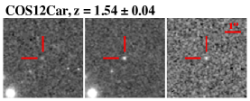
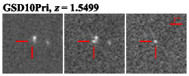
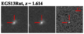
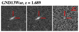
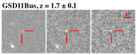
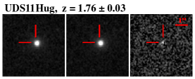
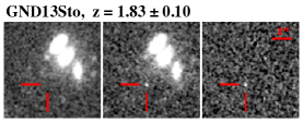
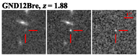
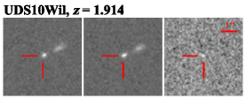
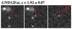
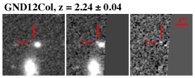
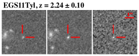
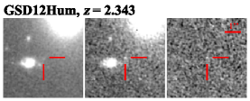
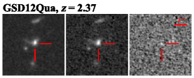
Figure 1.— Detection images for 14 SN from the CANDELS fields with redshifts $z>1.5$. Each image triplet shows H band (F160W) images with the template image on the left, the discovery epoch image in the middle and the difference image on the right. All images have a width of about 6 arcseconds, with North up and East to the left. The position of the SN is marked by (red) crosshairs in every frame. Discovery images for the other 51 SN with $z<1.5$ are provided in Appendix B.

To find SN candidates in the CANDELS WFC3-IR difference images, we used human searchers, who scanned each image by eye to detect significant deviations from the noise. We had $\sim$20 individuals regularly engaged in searching the CANDELS data, and searching tasks were assigned so that every WFC3-IR tile was examined by at least two people. Searchers recorded the position of all potential transient object detections, and assigned a quality grade. All transient sources receiving a high- or moderate-quality grade were carefully vetted to pare down to a list of transient sources that are very likely real SN. The criteria for inclusion in this SN candidate list are: (1) a profile consistent with a point source; (2) detected in the J+H difference image and also individually in both the J and H bands, (3) clean of evidence indicating that it could be a detector artifact (neighboring bad pixels, on the detector edge, etc). For the rates analysis presented here, we also require that the object reached its peak magnitude in IR bands after the HST template images were collected (i.e., we reject any SN that has less flux in the search epoch than in the template epoch).

Finally, we also discard a total of 6 objects that are positively classified as AGN. These 6 were located at the center of a host galaxy that has observational indicators to classify it as an AGN (x-ray emission, spectral line broadening, prior optical/IR variability, etc.). Our final sample contains 65 SN candidates that meet these requirements. Table 3 lists the 14 SN at redshifts $z>1.5$, and Table 9 in the Appendix lists the remaining 51 SN. In keeping with the practice of past HST SN surveys, we assign each SN a unique 8-digit name that indicates the field and the year of discovery, with the final 3 letters referencing our team’s internal “nickname” for each object. Figure 1 shows “postage stamp images” with the detection images for the 14 SN at $z>1.5$, and the remainder are in the Appendix, in Figures 5 and 6.

II.3. Follow-up Observations

Upon discovery, every SN was evaluated for possible follow-up observations with HST or ground-based telescopes. First, a redshift probability density function (pdf) was assigned, using pre-existing spectroscopy of the host galaxy when available and a photometric redshift (photo-z) when not. The photo-z estimates were derived from template fitting to the observed spectral energy distribution (SED) of each SN host galaxy (Dahlen et al. 2013). Then a preliminary SN classification (Ia or CC) was assigned by comparing the color and magnitude of the observed SN against a sample of synthetic SN with redshifts drawn from the best available redshift pdf. These synthetic SN were generated with the SuperNova ANAlysis software (SNANA; Kessler et al. 2009b) (see section IV for more details).

Any SN with a redshift $z>1$ and a color consistent with a SN Ia classification was then considered for possible follow-up observations with HST. Where necessary and whenever possible, the host galaxies of these high-priority targets were quickly observed (within $\sim$1 week of discovery) with ToO spectroscopic observations using ground-based observatories (primarily Gemini, Keck, and the Very Large Telescope (VLT)). The host galaxies of other SN candidates (CC SN and those with $z<1$) were targeted for later spectroscopic observations from the ground to determine precise redshifts, all reported in Table 4 (and in the Appendix Table 10).

Table 314 Supernovae with $z>1.5$ (see Appendix for the remainder)

Name	R.A. (J2000)	Decl. (J2000)	P(Ia$|$Dz)	P(Ia$|$Dhost)	z${}_{\mbox{\scriptsize SN}}$	($\pm$)	$z$ Source
COS12Car	10:00:14.726	$+$02:11:32.57	0.62 ${}^{+0.09}_{-0.36}$	0.80 ${}^{+0.00}_{-0.07}$	1.54	(0.04)	SN spec-z + SN phot-z
GSD10Pri	03:32:38.010	$-$27:46:39.08	1.00 ${}^{+0.00}_{-0.00}$	1.00 ${}^{+0.00}_{-0.00}$	1.545	(0.001)	host+SN spec-z
EGS13Rut	14:20:48.106	$+$53:04:22.12	1.00 ${}^{+0.00}_{-0.00}$	1.00 ${}^{+0.00}_{-0.00}$	1.614	(0.005)	host spec-z + SN phot-z
GND13War	12:36:54.761	$+$62:12:16.70	0.01 ${}^{+0.02}_{-0.01}$	0.01 ${}^{+0.00}_{-0.00}$	1.689	(0.005)	host spec-z
GSD11Bus	03:32:42.776	$-$27:48:07.10	0.00 ${}^{+0.00}_{-0.00}$	0.00 ${}^{+0.00}_{-0.00}$	1.7	(0.1)	host+SN phot-z
UDS11Hug	02:17:37.427	$-$05:08:41.43	0.82 ${}^{+0.05}_{-0.21}$	1.00 ${}^{+0.00}_{-0.00}$	1.761	(0.025)	host+SN phot-z
GND13Sto	12:37:16.778	$+$62:16:41.43	1.00 ${}^{+0.00}_{-0.00}$	1.00 ${}^{+0.00}_{-0.00}$	1.83	(0.10)	host+SN phot-z
GND12Bre	12:36:55.520	$+$62:13:58.82	0.00 ${}^{+0.00}_{-0.00}$	0.00 ${}^{+0.00}_{-0.00}$	1.880	(0.001)	host spec-z
UDS10Wil	02:17:46.336	$-$05:15:24.00	1.00 ${}^{+0.00}_{-0.00}$	1.00 ${}^{+0.00}_{-0.00}$	1.914	(0.001)	host+SN spec-z
GND12Fai	12:36:15.822	$+$62:15:56.50	0.00 ${}^{+0.00}_{-0.00}$	0.00 ${}^{+0.00}_{-0.00}$	1.92	(0.07)	host+SN phot-z
GND12Col	12:36:37.569	$+$62:18:32.93	1.00 ${}^{+0.00}_{-0.01}$	1.00 ${}^{+0.00}_{-0.00}$	2.24	(0.04)	host+SN phot-z
EGS11Tyl	14:20:12.944	$+$52:57:10.60	0.24 ${}^{+0.13}_{-0.15}$	0.57 ${}^{+0.03}_{-0.04}$	2.244	(0.095)	host+SN phot-z
GSD12Hum	03:32:15.500	$-$27:50:50.02	0.00 ${}^{+0.00}_{-0.00}$	0.00 ${}^{+0.00}_{-0.00}$	2.343	(0.001)	host spec-z
GSD12Qua	03:32:11.723	$-$27:49:11.72	0.00 ${}^{+0.00}_{-0.00}$	0.00 ${}^{+0.00}_{-0.00}$	2.370	(0.001)	host spec-z

Table 4Host galaxies of 14 Supernovae with $z>1.5$ (see Appendix B for the remainder)

SN	R.A. (J2000)	Decl. (J2000)	d[′′]	d[kpc]	Morph.	SED	z${}_{\mbox{host}}$	($\pm$)	$z$ Reference
COS12Car	$\cdots$	$\cdots$	$\cdots$	$\cdots$	$\cdots$	$\cdots$	$\cdots$	$\cdots$	$\cdots$
GSD10Pri	03:32:37.991	$-$27:46:38.69	0.46	9.6	i	SB	1.545	0.001	Frederiksen et al. (2012)
EGS13Rut	14:20:48.113	$+$53:04:22.07	0.08	1.7	d	A	1.614	0.005	HST+WFC3 (A.Riess)
GND13War	12:36:54.787	$+$62:12:16.60	0.21	4.3	di	SB	1.689	0.005	HST+WFC3 (B.Weiner)
GSD11Bus	03:32:42.776	$-$27:48:07.10	0.00	0.0	u	A	1.76	0.53	phot-z (T.Dahlen)
UDS11Hug	02:17:37.415	$-$05:08:41.53	0.21	4.2	s	P	1.82	0.13	phot-z (T.Dahlen)
GND13Sto	12:37:16.823	$+$62:16:42.65	1.26	25.5	u	A	1.8	1.2	phot-z (T.Dahlen)
GND12Bre	12:36:55.520	$+$62:13:58.79	0.03	0.6	i	SB	1.880	0.005	Keck+MOSFIRE (J. Trump)
UDS10Wil	02:17:46.332	$-$05:15:23.90	0.12	2.4	s	SB	1.914	0.001	Jones et al. (2013)
GND12Fai	12:36:15.934	$+$62:15:55.91	0.98	19.9	sd	SB	1.77	0.25	phot-z (T.Dahlen)
GND12Col	12:36:37.514	$+$62:18:32.66	0.47	9.6	s	A	2.1	0.2	phot-z (T.Dahlen)
EGS11Tyl	14:20:12.938	$+$52:57:10.62	0.06	1.2	sd	SB	1.95	0.45	phot-z (T.Dahlen)
GSD12Hum	03:32:15.585	$-$27:50:50.43	1.20	24.3	di	SB	2.343	0.001	Balestra et al. (2010)
GSD12Qua	03:32:11.713	$-$27:49:11.29	0.45	9.3	di	SB	2.370	0.001	VLT+Xshooter (J.Hjorth)

Some of the most promising candidates for classification as SN Ia at $z>1.5$ were selected for supplementary imaging and/or grism spectroscopy with HST. Two of these, SN GSD10Pri and UDS10Wil, have been presented elsewhere (Rodney et al. 2012; Jones et al. 2013). Due to the high cost of grism observations (at least 10 HST orbits are required to reach sufficient S/N in distant SN), we applied strict criteria for selecting grism targets: (1) best available redshift $z>1$, preferably $z>1.5$; (2) observed SN colors consistent with a (possibly reddened) SN Ia at that redshift; (3) observed SN magnitudes within $\sim$1.5 mag of a SN Ia at that redshift (i.e., using a very weak prior around a standard $\Lambda$CDM cosmology); (4) SN position allows for a grism observation without severe contamination.

Without a slit to isolate the SN light in WFC3-IR grism spectroscopy, a high-$z$ SN Ia candidate can most productively be observed if the trace of the SN spectrum can be positioned to avoid contamination from nearby galaxies. Thus, to satisfy the final criterion (4), the candidate must be well separated from the core of its host, or located in a host that is faint relative to the SN. We also require an orientation angle that avoids contamination of the SN spectral trace from the 0th order and 1st order light of other nearby stars and galaxies. Of course, this orientation must also be accessible to HST at the time of observation, with suitable guide stars in range. In practice, these criteria were satisfied for only 6 SN candidates. The results of those observations are described in Section VI. Another 37 CANDELS SN were followed with ToO imaging observations. These imaging targets included SN Ia candidates that satisfied some or all of the first three criteria, but were not suitable for grism observations, as well as some likely CC SN that we were able to include in the same field of view as those primary targets.

III. Detection Efficiency

Translating SN detections into a SN rate measurement requires characterization of the survey detection efficiency, i.e., the fraction of SN that are detected by our human searchers. This recovery fraction is most strongly influenced by the S/N of the object in the WFC3-IR difference images. The SN host galaxy is also an important factor affecting SN detectability, as we discuss further in Section III.1.

SN detection efficiency measurements as a function of magnitude in the “J+H” band, taken as an average of the measured F125W and F160W magnitudes. Each point represents the fraction of fake SN recovered by human searchers, with error bars indicating the standard deviation of the efficiency, computed using a Bayesian formalism (Paterno 2004). The best fit model is shown as a solid (green) line, with best-fit parameters listed in the lower left. For reference, the equivalent best-fit curves for the J and H bands individually are shown in blue dotted and red dashed lines, respectively. The horizontal and vertical lines mark the 50% efficiency point for J+H detections: $m_{50}=25.4$ mag. The top axis marks the approximate redshift of a normal SN Ia with average extinction ($A_{V}$=0.3) that would reach a peak brightness matching the J+H magnitude on the bottom axis.

To measure our SN detection efficiency and explore the associated systematic biases, we generated a catalog of 2,000 fake SN. The catalog was drawn from a SNANA Monte Carlo simulation, such that the F160W magnitudes fill out a uniform distribution covering the range $21<m_{H}<28$, and the $J-H$ colors were appropriate for Type Ia and Core Collapse SN in the redshift range $0.1<z<2.8$. Each fake SN was then assigned to a “host galaxy” drawn from catalogs of extended sources in the CANDELS fields. The separation from the host-galaxy center for each fake SN was then selected randomly from a normal distribution centered on 0 with a standard deviation of $2\times R_{50}$, where $R_{50}$ is the radius of an aperture containing 50% of the host-galaxy flux. This ensures that the fake SN very roughly follow the distribution of host light (Kelly et al. 2008).

With magnitudes, colors and positions defined, we generated synthetic PSFs for each fake SN using TinyTim, and planted them in the FLT images, as described in section II.1. As the searchers reviewed each difference image, they were unaware of the number, brightness, and location of the fake SN, so they recorded fake SN detections alongside detections of real SN. After completing each search, the fake SN detections (and non-detections) were used to calculate the recovery fraction.

Figure III shows the measured detection efficiency as a function of the “J+H” magnitude: the average of the F125W and F160W magnitudes. We fit the efficiency measurements with a functional form similar to that used by Sharon et al. (2007), but we use only a single parameter to characterize the exponential turnover, and we allow for the peak efficiency to plateau at a value less than unity:

$$\eta_{\rm det}(m)=\eta_{0}\times\left(1+\exp\left(\frac{m-m_{50}}{\tau}\right)\right)^{-1},$$ (1)

where $m$ is the apparent J+H magnitude, $\eta_{0}$ is the maximum efficiency, $m_{50}$ is the magnitude at which the efficiency curve passes through the 50% line, and $\tau$ characterizes the exponential roll-off. The best-fit curve shown in Figure III has $m_{50}$=25.4, $\tau$=0.23, and $\eta_{0}$=0.98.

III.1. Missing SN in Galaxy Cores

One concern for systematic bias entering into these detection efficiency measurements is the possibility that many SN are obscured by difference imaging artifacts in the cores of bright galaxies. The shot noise in these bright pixels is naturally higher than in the outskirts, as photon counts are elevated in both the search epoch and the template. Additionally, minor cross-epoch registration errors can result in some residual flux in galaxy cores. In the CANDELS survey data these effects are both exacerbated by the under-sampled PSF of our single-epoch WFC3-IR images, as we have only two dithers per filter.

Fraction of CANDELS galaxies showing IR core residuals as a function of redshift, as determined from visual inspection of difference images generated by the SN data processing pipeline.

As shown in Figure III, we have measured our maximum detection efficiency $\eta_{0}$ to be less than unity even for very bright SN, due to the fake SN that happen to land in the noisy cores of bright galaxies. Our SN rate measurements will therefore naturally account for a small fraction of SN that are missed in this manner. However, this built-in correction is only valid if the distribution of positions for the fake SN $-$ relative to their host-galaxy cores $-$ is closely matched to the true distribution of the SN Ia population. Furthermore, it requires that the galaxies chosen for “hosting” our fake SN are themselves representative of the population of SN Ia hosts. Our fake SN procedures were designed to meet these requirements at low and intermediate redshifts, but this does not necessarily carry over into the new high-$z$ regime.

To evaluate whether this effect might be introducing a strong bias at high-$z$, we visually inspected the CANDELS IR difference images and identified all galaxies that exhibited strong residuals. For each galaxy we tabulated the spectroscopic redshift or the best available photo-$z$ from CANDELS catalogs. Comparing this redshift distribution for core residuals against the count of all galaxies as a function of redshift gives us a measure of the fraction of (detected) galaxies that might obscure SN in their bright cores. As shown in Figure III.1, the fraction is less than $\sim 10\%$ for all redshifts above 0.01, and less than $\sim 2\%$ for $z>1$ – consistent with the value of $\eta_{0}$ measured from fake SN. This result suggests that any systematic bias from galaxy core residuals is very minor. Therefore, in the rates calculation we do not include any bias correction, and we do not add any contribution to the systematic uncertainty budget.

IV. Classification

To reach the final classification probabilities listed in Table 3 (and Table 9), we used a Bayesian analysis of the observed multi-color light curves. This photometric classification approach was used for our full sample of 65 SN, supplemented by spectroscopic evidence for 6 objects, as described in Section VI. An early version of this classifier was introduced in Jones et al. (2013) with the presentation of SN UDS10Wil. Here we will again briefly describe the classification procedure, emphasizing recent changes.

IV.1. The STARDUST Classifier

Our photometric classification approach uses SNANA to generate simulations of SN Ia and CC SN light curves. The SN Ia simulations use the SALT2 model (Guy et al. 2010), which has free parameters for the date of peak (MJD_pk), redshift ($z$), shape ($x_{1}$) and color ($\mathcal{C}$). The simulated CC SN are drawn from the SNANA library of 42 CC SN light curve templates (26 Type II and 16 Type Ib/c). These templates are derived from the SN samples of the Sloan Digital Sky Survey (Frieman et al. 2008; Sako et al. 2008; D’Andrea et al. 2010), Supernova Legacy Survey (Astier et al. 2006), and Carnegie Supernova Project (Hamuy et al. 2006; Stritzinger et al. 2009; Morrell 2012). Each CC SN template defines the underlying shape and color of the synthetic light curves, which is then modified with free parameters for the date of peak, redshift, host extinction ($A_{V}$), and luminosity ($\Delta$m, the shift in magnitudes relative to the peak of the assumed luminosity function). For this work, we fix the SALT2 model parameters $\alpha=0.135$ and $\beta=4.1$ (Scolnic:2013a), and for all simulated CC SNwe fix the extinction law to $R_{V}$=3.1.

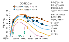
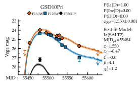
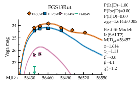
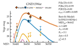
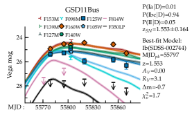
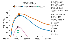
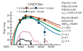
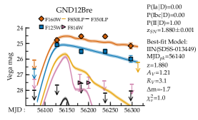
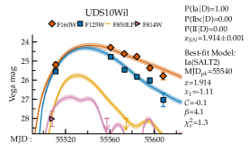
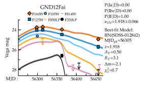
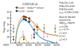
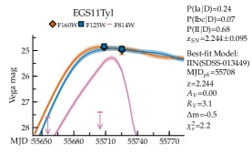
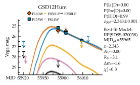
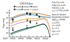
Figure 2.— Light curves of 14 SN with $z>1.5$. Each panel shows the observed photometry (in Vega mags) from CANDELS imaging with filled points and arrows for 3-$\sigma$ upper limits. Error bars are typically less than the size of the points. Curves depict the maximum probability light curve fit for the most probable SN class, as determined by STARDUST. Classification probablities and redshift as determined by STARDUST are listed on the right side of each panel, along with the parameters of the single model that delivers the highest posterior probability. Light curves for SN at $z<1.5$ are shown in Appendix B.

Comparing these synthetic SN to the observed light curves, we compute a likelihood using the $\chi^{2}$ statistic: $P({\bf D_{\rm LC}}|{\bf\theta},Ia)\propto\exp(-\chi^{2}/2)$, where the vector ${\bf D_{\rm LC}}$ is the observed SN light curve and the vector ${\bf\theta}$ gives the parameter values for each realization of the SNANA models. We then apply priors for each model parameter (see Graur et al. (2014) for a detailed description of these priors) as well as a redshift-dependent prior for the fraction of SN that are Type Ia: P(Ia,z) (see Section 3 IV.2 below). Finally, we derive the total posterior probability that each object is a SN Ia, $P(Ia|{\bf D_{\rm LC}})$, by marginalizing over the nuisance parameters, ${\bf\theta}$ and applying Bayes theorem :

$$P(Ia|{\bf D_{\rm LC}})=k_{\rm LC}^{-1}\int_{\bf\theta}P(Ia,z)P({\bf D_{\rm LC}}|{\bf\theta},Ia)d{\bf\theta}.$$ (2)

The normalization factor $k_{\rm LC}$ is defined by requiring that that posterior probabilities for all three primary SN classes (Ia,Ib/c,II) sum to unity. The custom-built software package that executes this procedure is named STARDUST: Supernova Taxonomy And Redshift Determination Using SNANA Templates. The STARDUST code will be presented in full and publicly released in a subsequent paper (Rodney et al., in prep).

There are two notable differences between the STARDUST classification procedure applied here and that described in Jones et al. (2013). First, in this work we do not use a free parameter for flux scaling, so the absolute values of the simulated SN fluxes are defined by the SN luminosity functions and cosmology ($\Omega_{\rm m}$=0.3,$\Omega_{\Lambda}$=0.7,$w$=-1) that are assumed in the SNANA simulations. To allow for some uncertainty in this baseline cosmology (or equivalently, introducing some increased scatter in the assumed SN luminosity functions) we include a non-zero model uncertainty term in the $\chi^{2}$ calculation. This is fixed at 8% of the simulated flux for SN Ia models and 10% for all CC SN models. Secondly, when the SN in question does not have a precise redshift from host-galaxy spectroscopy, we use the host galaxy’s photometric redshift probability distribution (photo-z pdf) as the redshift prior.

Column 4 of Table 3 (and Table 9 in the Appendix) presents the final SN classification probabilities, which will be used in Section VII for the SN Ia rate calculation. Figure 2 (and 7-9) shows the maximum likelihood light curve fit for each SN, along with the associated best-fit model parameters. As described below, the systematic uncertainties associated with each classification probability are determined by varying two key priors that are not tightly constrained by observations: the assumed fraction of SN that are of Type Ia and the distribution of host-galaxy extinction.

Deriving the redshift-dependent prior for SN class fractions. The top panel shows SN Ia rates and the middle panel shows CC SN rates. Both have observed rates plotted as open symbols. In the Ia case these are average values from all non-redundant field SN surveys. The CC SN rate points are the collection from Dahlen et al. (2012). In each panel the overlaid solid lines show three versions of a simple empirical model for the SN rates, and in the CC panel the magenta line traces the cosmic star-formation history (see text for details). The bottom panel plots the fraction of all SN explosions that are of Type Ia, derived from pairs of curves drawn from the top two panels and anchored to $25\pm 5\%$ at z=0 (Smartt et al. 2009; Li et al. 2011). These relative rate assumptions provide the high-, mid- and low-rate priors that are used to derive classification probabilities and associated uncertainties for observed SN.

IV.2. The Class Prior

As with any Bayesian classification approach, the STARDUST classifier requires an input prior that quantifies the expectation that any given SN is of Type Ia – before applying any information from the SN light curve. We first assume that our sample is composed entirely of “normal” SN, meaning that we assume no contamination from any other transient sources. This is a fairly safe assumption: AGN and variable stars are excluded by our discovery requirements, under-luminous SN like the .Ia (Bildsten et al. 2007) or Iax SN (Foley et al. 2013) are well below our detection threshold, and super-luminous SN (Gal-Yam 2012) have an intrinsic rate that is lower than that of normal SN by a factor of about 10⁴ (Quimby et al. 2011).

We then define a redshift-dependent class prior P(Ia,$z$) as the fraction of all normal SN at any given redshift $z$ that are Type Ia. Figure IV.1 shows the models used to define this prior and the associated systematic uncertainty. The baseline model (green curve) is anchored at z=0 by the measured Ia fraction (Smartt et al. 2009; Li et al. 2011), and then evolves at higher redshifts by following simple rate functions that match measured SN rates and theoretical expectations.

A more complete statistical treatment would define a large number of plausible models for the fraction of SN that are SN Ia, assigning each an appropriate weight based on current observations, and then marginalize over those many discrete priors to get a posterior probability that is not uniquely guided by the single choice of a baseline model. That approach is computationally expensive and will require further refinement of the STARDUST classifier. For this work, we have chosen to treat this choice of prior as a component of our systematic uncertainty budget. We take the baseline prior described above as our mid-rate model and then define two more models, labeled the high- and low-rate priors. These two respectively maximize and minimize the fraction of SN that are assumed to be of Type Ia at any given redshift, and are shown in Figure IV.1. These bounding models offer a conservative estimate of the systematic uncertainty, because they are at the extreme limit of plausibility (if either were correct it would imply that the constraints from past rate SN Ia measurements were all systematically wrong by more than $2\sigma$).

One might be concerned about the apparent circularity of using a redshift-dependent P(Ia,z) prior based on measured SN Ia rates in the service of a new SN Ia rate measurement. However, the bounding assumptions for our classification prior should ensure that our systematic uncertainty estimates account for this. To test that assertion, in Appendix A we evaluate an alternative prior that is based on the SN host galaxies and does not evolve with redshift. Tables 3 and 9 record the resulting STARDUST classifications using this modified prior as P(Ia$|$D_host) in column 5. Table 8 in the Appendix reports the final effect of this prior switch on the observed count of SN Ia and the volumetric rates.

Prior probability distributions for the SN host-galaxy extinction, as used in the STARDUST classifier code. The top panel shows the three priors applied to the SN Ia models, and the bottom panel shows the equivalent priors used for CC SN models. In both cases the high-dust model is shown as a red dashed line, the mid-dust model as a green solid line, and the low-dust model as a blue dash-dot line. Each model is composed of a Gaussian and/or an exponential function (see text for details) and the parameters for those components are listed in the legends. Each curve is labeled with its expectation value $\langle A_{\rm V}\rangle$, giving the “weighted average” of the host-galaxy extinction for that model.

IV.3. Host $A_{V}$ Distribution

Another prior that can strongly affect the final classification probabilities is the assumed distribution of host-galaxy extinctions, $P(\mbox{$A_{V}$})$. As with the SN Ia fraction prior, we employ a baseline assumption (our mid-dust model) and two bounding assumptions (high-dust and low-dust) to constrain the possible systematic bias.

In keeping with observations, our dust models assume that the CC SN population suffers from significantly more dust extinction than the SN Ia population, at all redshifts (e.g., Smartt et al. 2009; Drout et al. 2011; Kiewe et al. 2012; Mattila et al. 2012). Our three dust models are generated from the positive half of a Gaussian distribution centered at $\mbox{$A_{V}$}=0$ with dispersion $\sigma$, plus an exponential distribution of the form $e^{-A_{\rm V}/\tau}$. The parameter $\mathcal{R}_{0}$ gives the ratio of the height of the Gaussian to the height of the exponential, at $\mbox{$A_{V}$}=0$. The defining parameters and the expectation values for these three distributions are summarized in Fig IV.2.

When simulating SN Ia with the SALT2 model, the SN color is defined by the SALT2 $\mathcal{C}$ parameter. This color term comprises both the intrinsic SN color as well as reddening from host-galaxy dust. The distribution of $\mathcal{C}$ values can therefore be described as a convolution between a narrow Gaussian (the intrinsic dispersion of SN Ia colors) and a function describing the distribution of host-galaxy extinctions. Following Barbary et al. (2012) and Scolnic:2013a, we approximate the $A_{V}$ distributions of previous SN Ia studies by modifying the red side of the SALT2 $\mathcal{C}$ distribution so that the simulated SN colors match the output of that convolution.

Specifically, our high-dust model for SN Ia matches the baseline $A_{V}$ distribution used by Neill et al. (2006): a Gaussian with $\sigma=0.62$. The mid-dust model is equivalent to the exponential distribution of Kessler et al. (2009a): $P(\mbox{$A_{V}$})=e^{-A_{V}/\tau}$, with $\tau=0.33$. Our low-dust model for SN Ia assumes minimal dust extinction, using a narrow Gaussian with $\sigma=0.15$ plus a shallow exponential with $\tau=0.15$. A more complete treatment of host galaxy dust would include a prescription for the redshift-dependence of these extinction distributions, as SN hosts are expected to be dustier at redshifts approaching $z=2$ (Mannucci et al. 2007). As we will see in Section VII, this systematic uncertainty is not a dominant component of the error budget, so redshift dependence is left for future work.

To determine the combined systematic effects from the SN Ia fraction prior and the dust assumptions, we compute each SN classification probability 9 times: 3 for each SN rates prior $\times$ 3 for each dust model. The mid-rate $+$ mid-dust combination gives us our baseline classification probability, which dictates how much each individual SN contributes to the total count of observed SN Ia, $N_{\rm obs}$. The extrema from this set of 9 probabilities then provide the systematic classification errors, which propagate directly into the systematic uncertainty on the SN Ia rate.

IV.4. STARDUST Validation Test

A full investigation of the accuracy of the STARDUST classification code is beyond the scope of this paper. It is useful, however, to examine a simple validation test to demonstrate that this classifier is not grossly biased or ineffective. To that end, we have applied the STARDUST classifier to the “Gold” sample of 31 SN from the GOODS and PANS surveys (Strolger et al. 2004; Riess et al. 2007) that have spectroscopic classifications. These surveys were carried out using the HST ACS, and share many of the survey design characteristics of the CANDELS SN program. STARDUST correctly classifies 29 of the 31 SN (93.5%), using only their redshifts and photometric data. This demonstrates that we have a low false negative rate with STARDUST, i.e., we rarely misclassify a true SN Ia. Unfortunately, this validation test is not sensitive to false positives – true CC SN being misclassified as Type Ia – because we only have a single spectroscopically confirmed CC SN in this Gold sample. Preliminary testing of the STARDUST classifier using simulated SN suggests that the Ia sample purity for photometrically classified SN could be on the order of 95% (these validation tests will be presented in a future paper).

V. Host Galaxies

Host-galaxy information is recorded in Table 4 for the SN at $z>1.5$, and in the Appendix Table 10 for the low-redshift SN. As can be seen in Figure 1 (and Figures 5-6), most of the 65 CANDELS SN can be unambiguously associated with a host galaxy, because the host is isolated, or the SN is clearly embedded within the stellar light of a single galaxy. There are, however, a few exceptions.

For SN COS12Her, there are two host-galaxy candidates: the nearest and brightest has a photometric redshift of 0.403 ${}^{+0.04}_{-0.11}$, but the observed SN colors can not be adequately matched by any normal SN template in that redshift range. The second COS12Her host candidate has a photo-z=$1.10^{+0.16}_{-0.19}$. At this higher redshift, the STARDUST classifier finds a very good match to the observed light curve with a Type II-P template.

SN GND13Sto is separated by several arcseconds from all nearby galaxies. Of the 6 galaxies within 5 arcseconds of the SN position, 5 have a photo-z distribution that peaks close to z=1.8, including one with a spectroscopic redshift from the Spitzer Infrared Spectrograph of $z=1.80\pm 0.02$ (Murphy et al. 2009). This is suggestive of a small cluster or group of galaxies at that redshift, with SN GND13Sto possibly associated with a low surface brightness group member or tidal stream. Indeed, applying STARDUST to the well-sampled SN GND13Sto light curve (and allowing for a broad redshift range, z=1.8$\pm$1.2), we find the maximum likelihood match is a SN Ia template at z=1.86$\pm 0.05$.

There are four SN for which the host galaxy is barely detectable in the deep IR imaging mosaics from CANDELS. These are SN GND12Kin, EGS11Nix, GND13Gar, and GSD11Bus. All four of these objects lack a clear spectroscopic redshift from their host, so we are limited to using photometric redshifts for the STARDUST priors. In all of these cases, with STARDUST we find good template matches within the allowed redshift range.

V.1. Morphology and SED Type

The SN host galaxies (along with all CANDELS galaxies) were classified visually by members of the CANDELS team into three morphological categories: spheroid, disk, and irregular. Visual classifications were done using template images so that the presence of the SN did not bias the classification. Each galaxy can be assigned to multiple categories, so we also include two intermediate categories: spheroid+disk and disk+irregular. These morphological classes roughly correspond to broad bins over the Hubble sequence. This is appropriate for classifying galaxies at high redshift where distinguishing between, say, an E and an S0 galaxy is more difficult and less meaningful. Full details of the CANDELS morphological classification procedure will be presented in a forthcoming paper (Karteltepe, in prep).

We also record the “SED type” for each SN host galaxy, determined by matching the full galaxy SED against a set of templates, using the GOODZ code (Dahlen et al. 2010). The GOODZ template library is segregated into three groups, labeled according to the amount of ongoing star formation: passive (early type), active (late type), and starburst. We use the best-matching SED template for each CANDELS SN host galaxy to assign it to one of those bins.

For two of the SN (COS12Car and GND12Daw) there is no discernible host at the location of the SN and no nearby galaxy presents a plausible host candidate. For both of these objects we do have spectroscopic redshift information from the SN themselves, as detailed in Section VI. For the other 63 SN in our sample, 10 host galaxies are classified as spheroids, 15 as spheroid+disk, 17 as disk, 7 as disk+irregular, and 8 as irregular. For 6 of our SN, the host galaxy is detected, but is too faint for reliable visual classification, so we report the host morphology as “unclassifiable”. For the 63 objects with detectable host galaxies we have 2 passive, 24 active and 37 starburst-like SEDs.

VI. Grism Spectroscopy

Observed spectra and spectral template matches for four CANDELS SN. The spectra for GSD11Was (top left) and GND13Daw (top right) were collected using the G141 grism on HST’s WFC3-IR detector. The GND13Gar spectrum (lower left) used the ACS G800L grism, and the spectrum of COS12Car (lower right) combines observations from both the G102 and G141 WFC3 grisms. In each panel the observed flux is shown in gray, with binned points overlaid in blue, and the best-fitting template spectrum in red.

There are six objects in our sample for which we collected useful HST grism spectroscopy of the SN themselves. SN GSD10Pri, a Type Ia SN at $z=1.55$, was presented in Rodney et al. (2012) with an analysis of the host galaxy in Frederiksen et al. (2012). SN UDS11Wil, a Type Ia SN at $z=1.91$, was described in Jones et al. (2013). Figure VI presents grism spectra for the remaining four: SN GSD11Was, GND12Daw, GND13Gar and COS12Car. In all of these cases the signal to noise ratios and rest-frame wavelength coverage are insufficient for a purely spectroscopic classification. Rather, as with GSD10Pri and UDS11Wil, we used the spectroscopic information to supplement the STARDUST photometric classifier, leading to a more robust classification.

The host galaxy of SN GSD11Was has a photometric redshift of $z=1.04\pm 0.3$. We obtained a spectrum of SN GSD11Was with the WFC3-G141 grism, shown in Figure VI (top left). Here we can see hints of an absorption feature at $\sim$14,000 Å. At a redshift of $z\sim 1.3$ this feature can be explained as the characteristic SiII absorption trough seen at rest-frame $\sim$6150 Å in SN Ia spectra. Photometric classification of this SN with STARDUST agrees, finding the object is best matched by a SN Ia template at $z=1.3\pm 0.05$. (see the light curve plot in Appendix B, Figure 9).

SN GND12Daw, GND12Gar, and COS12Car all have no detectable host galaxy in any optical or NIR band, and no neighboring galaxies have redshifts that allow for acceptable light curve template matches in STARDUST. The most likely explanation is that these SN reside in very low surface brightness galaxies, too faint for detection even in our deep HST imaging.

The spectrum for GND12Daw shows hints of a broad emission feature at 12000 Å, which could be H$\alpha$ emission, if the object is at z=0.830. This could be interpreted as strong Balmer line emission from an otherwise very faint host galaxy, or it could be showing the H$\alpha$ emission from the SN itself – characteristic of Type II-P spectra. Given the very low signal to noise ratio in this spectrum (it was derived from just a single orbit of HST observations) this alone would be weak support. However, when allowing STARDUST to search over a redshift range $0.1<z<2.0$, we find that a Type II-P light curve template consistently provides the strongest match to the broad light curve shape of this SN, and the solution at $z\approx 0.8$ provides $>90\%$ of the total likelihood.

For GND12Gar (upper right) the absorption trough at $\sim$7700 Å provides a key observable that can anchor the fit and define the age of the SN. If this feature corresponds to Ca II absorption, then that would fix the object’s redshift to $z=1.07\pm 0.02$. At this redshift the light curve is matched very well by SN Ia templates, and no other redshift or SN class can provide a better light curve match.

The strongest spectral constraint for SN classification comes from SN COS12Car. For this object we have observations with both the WFC3-G102 and G141 grisms. Fitting the composite spectrum with the SuperNova IDentification (SNID) software (Blondin & Tonry 2007), we find the best template match is a Type Ia SN at z=1.59. Once again we find that the STARDUST photometric classification agrees well with this spectroscopic information: a SN Ia light curve at $z\approx 1.6$ provides the best available light curve template.

VII. The Volumetric SN Ia Rate

To convert the observed SN counts into a volumetric rate, we use an approach similar to Dahlen et al. (2008) and Rodney & Tonry (2010). We first divide up the detected SN into four redshift bins of width $\Delta z=0.5$. The total contribution to the SN Ia count from each observed SN is equal to the Ia classification probability for that object. For objects with uncertain redshifts, this fractional contribution is distributed over multiple redshift bins according to the integrated area of the redshift pdf. Adding up all the fractional counts gives us the total observed SN Ia count as a function of redshift: $N_{\rm obs}(z)$. Statistical uncertainties for each bin are defined by the points encompassing the central 68% of the Poisson distribution.

We then use Monte Carlo simulations to compute a “control count” for each bin, $N_{\rm ctrl}(z)$, which is the expected number of SN Ia that would be detected if the cosmic SN Ia explosion rate were constant for all redshifts at 1 SNuVol = $10^{-4}~{}\mbox{yr}^{-1}~{}\mbox{Mpc}^{-3}~{}{\mbox{h}_{70}}^{3}$. By simulating SN Ia light curves within the context of the CANDELS survey, the computation of $N_{\rm ctrl}(z)$ incorporates both the survey volume and the control time (the time interval over which any given SN is visible to our survey).

We again use SNANA as our simulation engine, this time generating 100,000 SN Ia based on the SALT2 light curve model (Guy et al. 2010). The light curve for each synthetic SN is determined by a set of 4 variables: date of peak brightness $mjd_{\rm pk}$, redshift $z$, SALT2 shape parameter $x_{1}$, and SALT2 color parameter $\mathcal{C}$. The $\mathcal{C}$ parameter in SALT2 includes both intrinsic SN color as well as reddening from host-galaxy dust. Each redshift $z$ is drawn from the range $0<z<2.5$, following the constant volumetric rate assumption. To translate this redshift into a luminosity distance, we use our baseline cosmology: $\Omega_{\rm m}$=0.3, $\Omega_{\Lambda}$=0.7, $w$=-1, $H_{0}$=70. Values for $x_{1}$ are drawn from a normal distribution with mean and dispersion from Kessler et al. (2009a): $\bar{x}_{1}=-0.13$, $\sigma_{x_{1}}=1.24$. The color parameters are draw from a bifurcated Gaussian distribution with $\bar{\mathcal{C}}=0.04$, $\sigma_{\mathcal{C}}^{-}=0.08$, and $\sigma_{\mathcal{C}}^{+}=0.25$ $-$ parameters that match the “mid-dust” model described in Section IV.3 and Figure IV.2.

To choose values for $mjd_{\rm pk}$ we first establish the width of the survey window at any given redshift. By examining simulated SN Ia light curves in F125W and F160W, we find $t_{\rm min}$ and $t_{\rm max}$, the minimum and maximum dates relative to peak for which each SN would be detectable to our survey. Here detectability is defined by measuring the change in flux relative to a template epoch 52 days prior, and requiring that the corresponding J+H magnitude is brighter than the 50% detection threshold seen in Figure III. The allowed range for the simulated $mjd_{\rm pk}$ values at redshift $z$ is then [MJD_first-$t_{\rm max}(z)$, MJD_last+$t_{\rm min}(z)$], where MJD_first and MJD_last are the epochs for the first and last search epoch, respectively. For each redshift, random $mjd_{\rm pk}$ values are then drawn from a flat distribution spanning this survey window.

Each synthetic SN is “observed” in the SNANA simulator using survey parameters that match the actual operations of the CANDELS program, as given in Tables 1 and 2. For the Wide fields (COSMOS, EGS, UDS and the wings of the GOODS fields) we only have a single search epoch, so these fields are simulated together as the “CANDELS-Wide” search field. The 10-epoch GOODS-S and GOODS-N Deep fields are treated separately, but all observational parameters are computed in the same way. Due to the excellent stability of the HST photometric system, we adopt a single set of average values for zero points and detector noise. The total area in each field reflects the area in which SN searching can be done, i.e., the area covered by the SN search epoch and at least one prior epoch. The cadence between epochs is nominally 52 days, but the actual separation in time varies from pointing to pointing due to HST scheduling constraints. For this simulation we use a mean cadence for each field and each epoch, weighted by the area available for SN searching. Finally, we use the detection efficiency curve of Figure III to define the probability of “detecting” each simulated SN in any given epoch.

Table 5Observed SN Ia Counts and the Volumetric Rate

	Observed Count				Control Count			SN Rate
Redshift	$N_{\rm obs}$	$\delta N_{\rm Poiss}$	$\delta N_{\rm syst}$		$N_{\rm ctrl}$	$\delta N_{\rm syst}$		SNR	$\delta$SNRstat	$\delta$SNRsyst
$0.25$	1.46	${}^{+2.46}_{-1.06}$	${}^{+0.48}_{-1.44}$		4.10	${}^{+0.01}_{-0.04}$		0.36	${}^{+0.60}_{-0.26}$	${}^{+0.12}_{-0.35}$
$0.75$	7.19	${}^{+3.80}_{-2.62}$	${}^{+1.94}_{-2.54}$		14.11	${}^{+0.53}_{-1.71}$		0.51	${}^{+0.27}_{-0.19}$	${}^{+0.23}_{-0.19}$
$1.25$	8.47	${}^{+4.02}_{-2.85}$	${}^{+0.45}_{-2.04}$		13.16	${}^{+2.46}_{-4.05}$		0.64	${}^{+0.31}_{-0.22}$	${}^{+0.34}_{-0.23}$
$1.75$	5.54	${}^{+3.49}_{-2.28}$	${}^{+0.17}_{-0.61}$		7.67	${}^{+3.47}_{-2.99}$		0.72	${}^{+0.45}_{-0.30}$	${}^{+0.50}_{-0.28}$
$2.25$	1.24	${}^{+2.39}_{-0.96}$	${}^{+0.13}_{-0.16}$		2.52	${}^{+1.72}_{-1.07}$		0.49	${}^{+0.95}_{-0.38}$	${}^{+0.45}_{-0.24}$

Counting the number of detected synthetic SN in each redshift bin gives us the control count, which carries units of SNuVol^-1. The observed volumetric rate of SN Ia explosions is simply the ratio

$${\rm SNR}_{\rm Ia}(z)=\frac{N_{\rm obs}(z)}{N_{\rm ctrl}(z)}$$ (3)

The measured values for $N_{\rm obs}(z)$, $N_{\rm ctrl}(z)$, and SNR($z$) from the CANDELS survey are given in Table 5 along with uncertainty estimates due to statistical noise (Poisson errors) and systematic biases. The total sample size is quite small, with only $\sim$21 SN Ia across all redshifts and fewer than 7 in each bin. This means that the statistical errors are substantial, roughly equal to or greater than the systematic uncertainties in every redshift bin. One cannot infer a clear trend with redshift from these data alone, but rather we must evaluate them within the context of other rates measurements and SN Ia progenitor models.

VII.1. Systematic Uncertainties

In preceding sections we have considered three principal sources of systematic biases: (1) missing SN detections due to subtraction artifacts in the cores of bright galaxies, (2) the assumed fraction of SN that are of Type Ia as a function of redshift, and (3) the assumed distribution of host-galaxy dust extinction values. We have determined that bias from the first source is negligible. The second is examined in more detail in Appendix A, and is reflected in the systematic uncertainty estimates for the count of observed SN Ia (column 4 of Table 5). The third item also affects the control count (column 6).

Other potential sources of systematic bias include: errors in the luminosity functions for SN sub-classes, biases in the SN Ia model or the CC SN template libraries, and peculiar detection biases from individual human searchers. For this work, these contributions to the systematic error budget are assumed to be insignificant. Future analysis with the full CANDELS+CLASH sample will revisit this assumption and evaluate these systematic error sources.

VIII. Testing SN Ia Progenitor Models

The measurement of volumetric SN Ia rates at high redshift is principally motivated by two astrophysical investigations. First, it directly informs our understanding of the cosmic enrichment history, as SN Ia are a primary source for Fe-group elements in the universe (e.g., Wiersma et al. 2011). Secondly, by measuring the delay between star formation and SN explosion through the DTD formalism, one can draw inferences about the nature of SN Ia progenitor systems. In this work we limit our discussion to the latter, beginning with a comparison to other published SN Ia rates, then evaluating new constraints on progenitor models and finally making a projection toward future improvements.

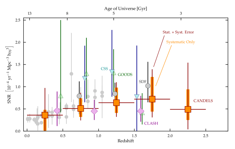
Figure 3.— Measured SNIa rates from CANDELS and other surveys. The CANDELS volumetric SN Ia rates measurements are shown as large orange squares, spanning 5 redshift bins of width dz=0.5. For these CANDELS points, the systematic uncertainties are shown as broad orange bars, while the thin vertical error bars show the combined systematic and statistical uncertainty. Four other high-redshift SN surveys are highlighted: gray circles for the Subaru Deep Field (SDF Graur et al. 2011), blue downward triangles for volumetric (not cluster) rates from the Cluster Supernova Survey (CSS Barbary et al. 2012), green upward triangles for the GOODS and PANS surveys (Dahlen et al. 2008), and magenta diamonds for the CLASH survey (Graur et al. 2014). Assorted ground-based surveys plotted as gray circles, as in Figure I.

VIII.1. Comparison to Earlier Rate Measurements

Figure 3 presents the CANDELS SN Ia rates within the context of other rates measurements from the literature. The CANDELS rate measurements are shown in 5 bins of width $\Delta z=0.5$ as large orange squares. Rate measurements from 13 ground-based surveys are plotted as small gray circles, reaching out to z=1.1. Four surveys that have previously extended the rate measurements to $z\approx 1.5$ are highlighted with larger colored points (see caption for details).

As with past HST surveys, our survey volume is too small to add any useful new information at $z<1$, but the general agreement with ground-based surveys is an important validation that our rate measurements are realistic. For a more informative comparison, we turn now to the high-$z$ side of the plot.

Before CANDELS and CLASH, there were just three surveys with any SN Ia rate measurements above z$\approx$1.2. First were the GOODS SN surveys, which used the HST ACS camera to measure the SN Ia rate to $z\approx 1.8$ (GOODS Strolger et al. 2004; Dahlen et al. 2004). These data were interpreted as showing a flattening or a downturn in the SNR($z$) at $z>1.2$, a trend that garnered support from additional HST observations and independent analysis (Dahlen et al. 2008; Kuznetsova et al. 2008), including another ACS program, the Cluster Supernova Survey (CSS Barbary et al. 2012). Ground-based rate measurements from the Subaru Deep Field (SDF) survey also reached out to $z\approx 1.8$, though these were more susceptible to systematic biases due to the absence of light curve information and spectroscopy for SN classification (Poznanski et al. 2007; Graur et al. 2011). As the CANDELS and CLASH surveys began, it was still an open question as to whether we had now seen the peak in the SN Ia rate, or if it was continuing to rise beyond $z\approx 1.2$.

The GOODS, CSS and SDF surveys all used optical bands that correspond to rest-frame near-UV wavelengths at high redshift. For a SN at redshift $z\approx 1.5$, observations in the $z$ band ($\sim 9000$ Å) are sampling the rest-frame U band, while the observer’s $i$ band ($\sim 8000$ Å) reaches well into the rest-frame near-ultraviolet. At these wavelengths the available SN light curve templates for use in photometric classification are poor, because most nearby SN surveys do not observe SN in the UV. Both SN Ia and CC SN also exhibit more natural heterogeneity at these blue wavelengths, and this is all compounded by a greater sensitivity to dust obscuration in the UV. Thus, optical-wavelength surveys were more susceptible to both of the components that dominate the systematic uncertainties of high-$z$ SN Ia rate measurements: classification bias and dust obscuration. By contrast, the CANDELS survey utilized the $J$ and $H$ IR bands that sample rest-frame optical wavelengths, even out to redshift $z\approx 2.5$. The CANDELS rates should therefore be less strongly affected by those systematic biases.

At $z=1.25$ the CANDELS rate is substantially lower than all past measurements, though still consistent at the 1–2$\sigma$ level. The CANDELS rate then climbs slightly in the bin at $z=1.75$, where it is completely consistent with past measurements. CANDELS is the only survey with any detections beyond $z=2$, and there we have only a single object with a strong probability of being a SN Ia (SN GND12Col in the GOODS-N field, at $z\approx 2.24$). The rate formally shows a decline to $z=2.25$, although this change is much smaller than the uncertainties. The CANDELS rates are fully consistent at all redshifts with the similarly derived rates from CLASH, which are also quite low relative to past surveys (Graur et al. 2014).

Due to the small sample sizes and large uncertainties, none of these individual high-$z$ surveys has sufficient precision to clearly delineate the shape of the SNR($z$) curve. From Figure 3 we can only say that the SN Ia rate rises steadily to $z\approx 1.2$, and then is flat or slowly declining at redshifts $z>1.2$.

Each independent analysis of SN Ia rates makes slightly different assumptions about host-galaxy extinction and each takes a different approach to SN classification. These differences become particularly important at $z>1$ where observed rates are dominated by HST SN surveys, which have much less complete spectroscopic information. Here the potential for systematic biases is much greater as a larger fraction of SN classifications and host-galaxy redshifts rely on photometric data alone.

An optimal approach would be to effectively treat the past decade of HST SN surveys as a single composite survey. One could compute the rates from all the HST SN surveys together, using the same SN classifier(s), consistent models for (redshift-dependent) host-galaxy extinction, and the best available host-galaxy redshift information. Such an effort is beyond the scope of this work, but will be an important contribution for future DTD tests.

VIII.2. Isolating the Prompt SN Ia Fraction

To examine how the observed SN Ia rate can inform the modeling of SN Ia progenitors, we will employ a simple toy model, motivated by a variety of recent observations and theoretical predictions. For a complementary analysis using DTD predictions from binary population synthesis modeling, see Graur et al. (2014). Multiple lines of evidence now suggest that the overall shape of the SN Ia DTD follows a $t^{-1}$ power law for times $t>500$ Myr (see Maoz & Mannucci 2012, for a recent review). At short delays, $t<500$ Myr, the evidence is much less definitive, and this is the region where the CANDELS observations may provide unique new insight. Thus, our primary question is: What fraction of SN Ia explode within 500 Myr of their formation?.

To isolate this “prompt SN Ia fraction”, we define a bifurcated DTD model: the long-delay component follows a $t^{-1}$ distribution for all times $t>500$ Myr, and the prompt component is set to be constant with time for $t<500$ Myr, down to a lower limit of $t_{\rm min}=40$ Myr (the shortest possible time to reach explosion, Belczynski et al. 2005):

$${\rm SNR}(t)=\begin{cases}0&\text{for $t<0.04$ Gyr},\\ K\,\eta_{\rm Ia}\,\frac{f_{P}}{1-f_{P}}&\text{for $0.04<t<0.5$ Gyr},\\ \eta_{\rm Ia}\,t^{-1}&\text{for $t>0.5$ Gyr},\\ \end{cases}$$ (4)

Here $\eta_{\rm Ia}$ indicates the efficiency of generating SN Ia progenitor systems, in units of SN Ia yr^-1 M_⊙^-1, and $f_{P}$ sets the fraction of all SN Ia that arise from the prompt channel. The constant K is defined by the time thresholds that delineate this model:

$$K=\ln(t_{\rm max}/t_{1})/(t_{1}-t_{\rm min}),$$ (5)

where $t_{\rm min}=0.04$ Gyr as defined above, $t_{1}=0.5$ Gyr marks the abrupt transition from the the constant rate to the power law, and $t_{\rm max}=13.3$ Gyr is the maximum age of a WD in the current universe – using our assumed $\Lambda$CDM cosmology and assuming star formation began at $z=20$. For these values, we have $K=7.132$. With this simple DTD model, we can allow $\eta_{\rm Ia}$ and $f_{P}$ to be free parameters, and fit to the data to find the observed efficiency and prompt Ia fraction.

The cosmic star-formation rate (CSFR) as a function of redshift. Points show the compilation of recent CSFR measurements from (Behroozi et al. 2013), adopting from those authors the corrections for dust attenuation and more realistic systematic errors. The solid line shows the best-fit double-power law model from (Behroozi et al. 2013), and the shaded region demarcates the 1-$\sigma$ systematic uncertainties.

To convert from this DTD model into a prediction for SN Ia rates, we convolve this DTD with a parameterized representation of the cosmic star-formation history, giving us a prediction for the observable SNR($z$). For this exercise we use the recent compilation of measurements of the cosmic star-formation rate ($CSFR(z)$) from Behroozi et al. (2013), shown in Figure VIII.2. The precise shape of the CSFR curve at $z>2$ is still a matter of debate, but for our purposes here we take the Behroozi et al. curve and associated systematic uncertainties to be representative of the current state of the art (but see Graur et al. 2014, for further evaluation of SFH variation).

The construction of our bifurcated DTD model is reminiscent of the two-component “A+B” model (Mannucci et al. 2005; Scannapieco & Bildsten 2005), but it has closer ties to recent theoretical predictions from binary population synthesis models. For example, Ruiter et al. (2013) found that a “violent merger” DD model predicts a $t^{-1}$ power law shape for long delay SN, but also includes a very prompt component that arises from a distinct subset of binary systems. A separate prompt channel for SN Ia explosions could also arise from a single-degenerate pathway with a helium-star donor (Wang et al. 2009; Claeys et al. 2014).

VIII.3. DTD model fitting results

To find the most likely values for our two parameters $\eta_{\rm Ia}$ and $f_{P}$, we use three SN Ia rate data sets. First we define the “All” data set, utilizing all available (non-redundant) volumetric rate measurements from the literature (see Graur et al. 2014, for a compilation table). Secondly, our “Ground” subsample picks out the 13 independent rate measurements from ground-based surveys. Finally, our “CANDELS+CLASH” sample isolates those 2 companion HST surveys.

The first three columns of Table  6 summarize the maximum likelihood values for our DTD parameters $\eta_{\rm Ia}$ and $f_{P}$, when fitting to each of these subsamples. When using all of the available SN Ia survey data, we find $\eta_{\rm Ia}=\left(1.60\begin{subarray}{c}\pm\\ \mbox{\scalebox{0.45}{stat}}\end{subarray}^{0.24}_{0.236}\begin{subarray}{c}\pm\\ \mbox{\scalebox{0.45}{sys}}\end{subarray}^{0.25}_{0.59}\right)\times 10^{-4}$ SN Ia yr^-1 M_⊙^-1 and $f_{P}$=0.53 $\begin{subarray}{c}\pm\\ \mbox{\scalebox{0.45}{stat}}\end{subarray}$${}^{0.09}_{0.10}$ $\begin{subarray}{c}\pm\\ \mbox{\scalebox{0.45}{sys}}\end{subarray}$${}^{0.10}_{0.26}$.

Fitting to the ground-based data alone, we find very similar best-fit parameters, with the prompt SN Ia fraction inching up to $f_{P}$=0.59 and the efficiency remaining at $\eta_{\rm Ia}\approx 1.5$. When we isolate the HST CANDELS and CLASH surveys, we get much larger uncertainties, but perhaps also a subtle hint at tension between the ground- and HST-based results: from the CANDELS+CLASH sample we get $f_{P}$=0.21 $\begin{subarray}{c}\pm\\ \mbox{\scalebox{0.45}{stat}}\end{subarray}$${}^{0.34}_{0.21}$ $\begin{subarray}{c}\pm\\ \mbox{\scalebox{0.45}{sys}}\end{subarray}$${}^{0.49}_{0.12}$. The difference in these best-fit parameters reflects a (very) mild disagreement between the ground-based, primarily low-$z$ rate measurements and the high-$z$ constraints from HST.

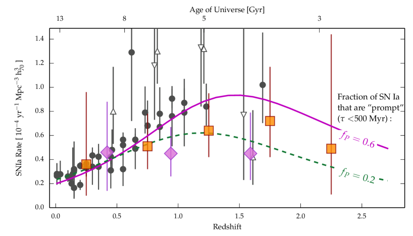
Figure 4.— Comparing observed SN rates against DTD models. Grey markers show the collection of rates from the literature, with filled points for the ground-based surveys, and open symbols for past HST surveys. As in Figure 3, large purple diamonds show the CLASH rates from Graur et al. (2014) and large orange squares show the CANDELS rates from this work. In this figure vertical error bars show only the statistical uncertainties. Two curves show the SN Ia rates predicted by assuming a DTD that is proportional to $t^{-1}$ for all times above 500 Myr, but with different assumptions for the fraction of SN Ia that are prompt. The magenta solid line shows the best-fit to the ground-based data (solid grey points), which has $\sim$60% of all SN Ia exploding within 500 Myr of birth. The green dashed line is the best-fit model when using the CANDELS+CLASH data alone, for which the prompt SN Ia fraction is $\sim$20%.

Table 6Observational Constraints on the SN Ia Delay Time Distribution

Sample	$\eta_{Ia}$	$f_{P}$	NIa/M∗	NIa/M∗
	$[10^{-4}\mbox{M${}_{\odot}$}^{-1}yr^{-1}]$		$[10^{-3}\mbox{M${}_{\odot}$}^{-1}]$	$[10^{-3}\mbox{M${}_{\odot}$}^{-1}]$
CANDELS & CLASH	2.25 ${}^{+1.36}_{-1.18}$ ${}^{+0.72}_{-0.15}$	0.21 ${}^{+0.34}_{-0.21}$ ${}^{+0.49}_{-0.12}$	0.79 ${}^{+1.52}_{-0.50}$ ${}^{+2.11}_{-0.16}$	0.60 ${}^{+0.97}_{-0.37}$ ${}^{+0.87}_{-0.46}$
Ground	1.38 ${}^{+0.24}_{-0.23}$ ${}^{+0.43}_{-0.21}$	0.59 ${}^{+0.09}_{-0.10}$ ${}^{+0.05}_{-0.04}$	0.84 ${}^{+0.39}_{-0.27}$ ${}^{+0.44}_{-0.54}$	$\cdots$
All	1.60 ${}^{+0.24}_{-0.23}$ ${}^{+0.25}_{-0.59}$	0.53 ${}^{+0.09}_{-0.10}$ ${}^{+0.10}_{-0.26}$	0.98 ${}^{+0.43}_{-0.30}$ ${}^{+0.87}_{-0.46}$	0.79 ${}^{+0.88}_{-0.72}$ ${}^{+1.09}_{-0.75}$

Constraints on the DTD normalization factor and the fraction of SN Ia that are prompt explosions. Contours show the 68% and 95% confidence regions for the baseline assumptions (mid-dust, mid-rates) in the $\eta_{\rm Ia}$ vs. $f_{P}$ parameter space. The background color map indicates the time-integrated SN Ia efficiency, $N_{\rm Ia}/M_{*}$, for each point in that parameter space. Dashed contours show the confidence regions derived from only CANDELS+CLASH data, reaching to $z\approx 2.5$. Solid contours are from the collection of all ground-based SN surveys, dominated by measurements at $z<1$.

The source of this deviation is easily seen in Figure 4, where we plot two SNR($z$) curves derived from the bifurcated DTD model. The (magenta) solid line shows the best fit to the ground based data alone, with $f_{P}$=0.6. The (green) dashed line sets the prompt fraction to 20%, the best fit value for the CANDELS+CLASH data sample. These two HST surveys find a relatively low SN Ia rate at all redshifts $z\gtrsim 1$, which pulls the best-fit curve downward at high redshift, leading to the low best-fit $f_{P}$. We can also see the slight tension between ground and recent HST measures in Figure VIII.3, where we show confidence regions in the $\eta_{\rm Ia}$ vs. $f_{P}$ parameter space. The 68% contours from the ground- and HST-based surveys fall just short of overlapping. This discrepancy is only slightly above 1$\sigma$ in significance, and comes with all the caveats cited above regarding the method for combining data from disparate surveys. Nevertheless, these HST data do sample the redshift range with the greatest leverage for constraining $f_{P}$, so the scarcity of high-$z$ SN Ia detections in multiple HST surveys should not be discounted.

Table  6 and Figure VIII.3 also present the total number of SN Ia per stellar mass, $N_{\rm Ia}/M_{*}$. This is computed by integrating the SN Ia rate over a Hubble time, and dividing by the total mass of formed stars. For the denominator, we take the integral of the Behroozi et al. (2013) $CSFR(z)$ curve from Figure VIII.2 (which assumes a Chabrier (2003) stellar initial mass function). To get the numerator – the total number of SN Ia explosions in a Hubble time – we can integrate the best-fit DTD-based SNR($z$) model for each subsample of rates measurements. Those values are reported in the fourth column of Table 6. In the fifth column we list an alternative calculation, now directly integrating the SNR($z$) data, without reference to any DTD model. This latter approach yields a much less precise constraint, but it is more appropriate for use as a test of progenitor models, because it does not presuppose any particular shape for the DTD. Note that we do not measure a data-only constraint from the ground-based subsample because it does not reach a sufficiently high redshift.

Figure VIII.3 shows a color map in the background, reflecting the variation of $N_{\rm Ia}/M_{*}$ within the $\eta_{\rm Ia}-f_{P}$ plane (assuming that the DTD follows our two-component toy model). The contours derived from both the ground-based and HST surveys are roughly aligned along lines of constant $N_{\rm Ia}/M_{*}$ (a single-color ridge in the color map). Hence the relatively tight model-dependent constraints on $N_{\rm Ia}/M_{*}$ as reported in column 4 of Table 6.

All of the above $N_{\rm Ia}/M_{*}$ measurements are consistent with a value of roughly $1\times 10^{-3}\mbox{M${}_{\odot}$}^{-1}$. This is fully consistent with past measures of the volumetric rates, using similar stellar IMF assumptions (e.g., Graur et al. 2011). Other observational constraints, such as cluster SN Ia rates, have recently found values closer to $2\times 10^{-3}\mbox{M${}_{\odot}$}^{-1}$ (Maoz & Badenes 2010) – still consistent within the large error bars. However, theoretical predictions from binary population synthesis models are frequently lower by factors of 10 or more (Bours et al. 2013). This discrepancy between theory and observation remains one of the key concerns in the SN Ia progenitor problem.

VIII.4. Interpretation and Speculation

As described above, our analysis of all available SN Ia rates measurements suggests that the fraction of SN Ia explosions occurring $<$500 Myr after formation is $f_{P}$$\approx$50%. This observed value of $f_{P}$ is broadly consistent with the simplistic assumption of a t^-1 DTD that continues without truncation all the way down to 40 Myr, which yields $f_{P}$=0.43. A prompt fraction close to 50% is also observationally supported by several lines of evidence in the local universe. Mannucci et al. (2006) first proposed that roughly half of all SN Ia explode promptly after formation, based on observations of SN Ia host galaxies at low redshift. Building on that work, Raskin et al. (2009) used measurements of low-$z$ SN Ia environments on sub-galactic scales to infer that most of those prompt SN Ia explode at $200-500$ Myr. Mennekens et al. (2013) used binary population synthesis (BPS) to predict the distribution of chemical enrichment in our galaxy over time. Comparing this to observations of [Fe/H] in nearby G-dwarfs, they infer that prompt explosions must make up a large fraction of the SN Ia population (and thereby contribute to rapid galactic enrichment).

Can this measurement of the prompt SN Ia fraction be used to distinguish SD and DD progenitor models? BPS calculations generally agree that SD pathways preferentially generate prompt SN Ia explosions. In particular, SD progenitor models in which the companion is a naked He star are found to peak at $t\approx 100$ Myr after formation, while those with a normal main sequence or giant companion preferentially explode at $200-500$ Myr (Wang et al. 2009; Mennekens et al. 2010; Greggio 2010; Claeys et al. 2014). Some BPS modeling also finds that DD progenitors could contribute substantially to the population of SN Ia explosions younger than 500 Myr (Ruiter et al. 2009; Greggio 2010; Ruiter et al. 2013), although recent work by Claeys et al. (2014) suggests that the DD pathway does not dominate the DTD until $t>500$ Myr. At the moment, we can only say that a prompt fraction $f_{P}$$\approx$50% is commonly predicted by models that include both SD and DD progenitors – but it may be possible in a pure DD model as well.

When we analyze the HST sample in isolation, we find a hint that $f_{P}$ could be closer to $\sim$20%, though further analysis and a larger SN Ia sample will be needed to improve this measurement. Let us indulge in a bit of speculation and suppose that these future improvements confirm that $f_{P}$ is close to 20% at high redshifts. We would then need a theoretical explanation for how the prompt component of the SN Ia population could be suppressed at redshifts $z>1.5$. One possible explanation would be that the prompt SN Ia component is dominated by a SD progenitor pathway with a strong metallicity dependence. Such a metallicity dependence has been proposed by requiring an optically thick wind from the WD to regulate the mass transfer rate, allowing the WD to grow to the Chandrasekhar mass limit (Hachisu et al. 1996, 1999). This wind would be absent in low metallicity WDs, resulting in a suppression of prompt SN Ia explosions in the early universe (Kobayashi et al. 1998; Kobayashi & Nomoto 2009). No such metallicity threshold is expected for DD models, so this scenario could provide a clean way to disentangle the relative contributions of those two progenitor pathways.

IX. Summary

We have presented a sample of 65 SN from the 5 CANDELS fields. This sample, collected in concert with the CLASH SN search, is the first to extend SN Ia detections beyond $z=2$, and the first to detect SN at $z\approx 1.5$ in rest-frame optical bands. These SN have been classified primarily through the application of STARDUST, a new Bayesian photometric classifier that is optimized for working with light curves of high-redshift SN. We have spectroscopic redshifts from the SN and/or host galaxy for 82% of the sample (53 of 65), although we rely on photometric redshifts for 43% of the SN at $z>1.5$ (6 of 14). Our SN classification probabilities are in general tightly constrained by well-sampled light curves, rest-frame UV-optical colors, and well defined redshifts. The primary sources for potential systematic biases in our classifications are 1) a redshift-dependent prior describing the relative fraction of SN that are Type Ia, and 2) the assumed distribution of dust extinction values. For the former, a test using host-galaxy information to replace the class prior indicates that our systematic uncertainty estimates are appropriate.

From the CANDELS SN sample we have measured the volumetric SN Ia rate in 5 redshift bins reaching to $z=2.5$. We find that the CANDELS SN Ia rate measurement at $z\approx 1.25$ is a factor of 2 lower ($\sim 2\sigma$) than past HST rates measurements at the same redshift (Dahlen et al. 2008; Barbary et al. 2012), but is consistent with the concurrently measured SN Ia rates from CLASH (Graur et al. 2014). We attribute this discrepancy to Poisson noise, due to the very small sample sizes in all of these HST surveys. At higher redshifts the CANDELS rate measurements remain approximately flat with redshift.

Combining these CANDELS results with other surveys from HST and from the ground, we have examined the constraints that can be placed on SN Ia DTD models (Table 6, Figure 4). We have invoked a simple two-component model with a $t^{-1}$ distribution for long delay times ($t>500$ Myr), and a constant rate at shorter times. We find that the ground-based rates (primarily at $z<1$) and the full sample of all available SN Ia rates both are best matched with a prompt SN Ia fraction of $f_{P}=0.5$. When the CANDELS+CLASH surveys are analyzed in isolation, the best fit for the prompt SN Ia fraction falls to $f_{P}=0.21$${}^{+0.34}_{-0.21}$${}^{+0.49}_{-0.12}$. This is substantially lower, but with very large error bars.

Collectively, the constraints from all available volumetric SN data indicate that the prompt SN Ia fraction can not be much larger than about 60%. As described above, there is room for substantial improvement in our measurement of the prompt SN Ia fraction – without needing to acquire more data. Systematic uncertainties can be reduced (or at least better understood) by combining the existing HST surveys in a composite analysis that handles SN classification and dust obscuration in a consistent manner. Increasing the high-$z$ SN Ia sample size would also help, of course. The HST Frontier Fields initiative will provide the next opportunity for new high-$z$ SN discoveries. This program will utilize $\sim$900 orbits of HST observations for very deep imaging of 6 massive galaxy clusters over 3 years. An approved HST program for SN discovery and follow-up (PI:Rodney, PID:13386) is expected to deliver a SN Ia sample that reaches out to $z\approx 3$.

We dedicate this work to the memory of our friend and colleague, Tomas Dahlen. He is dearly missed.

The authors would like to thank the referee, Massimo Della Valle, for helpful comments and suggestions. We are also grateful to the STScI science support staff for their extraordinary efforts in executing the MCT programs, especially program coordinators Patricia Royle and Beth Perriello, as well as the entire STScI scheduling team that made our HST ToO program possible. We give thanks to Kelsey Clubb, Ori Fox, Patrick Kelly, Isaac Shivvers, Brad Tucker, and WeiKang Zheng for assistance with some of the Keck observations; to Ismael Botti, Alice Mortlock, and Omar Almaini for redshift and AGN classifications of SN candidates in the UDS field; to Stephane Blondin for VLT spectral reductions and assistance with SNID modifications; to Jennifer Lotz and Ryan Foley for discussions improving the measurement and application of SN host-galaxy morphologies; and to Thomas Holoien and Mark Ziegler for “fake SN” searching assistance.

The CANDELS and SN-MCT programs were supported by NASA through HST grants GO-12060 and GO-12099 (respectively) from STScI. Support for S.A.R. was provided by NASA through Hubble Fellowship grant HST-HF-51312. Support for this research at Rutgers University was provided in part by NSF CAREER award AST-0847157 to S.W.J. A.V.F. is also grateful for the support of National Science Foundation (NSF) grant AST-1211916, the TABASGO Foundation, and the Christopher R. Redlich Fund. The Dark Cosmology Centre is supported by the Danish National Research Foundation. R.P.K. thanks the National Science Foundation for AST-1211196, and the John Simon Guggenheim Foundation for support. This work was supported by NASA Keck PI Data Awards (to Rutgers University, PI: S.W.J.), administered by the NASA Exoplanet Science Institute. J.M.S. is supported by an NSF Astronomy and Astrophysics Postdoctoral Fellowship under award AST-1302771. S.G.W. is supported by the NSF Graduate Research Fellowship under Grant No. DGE-1232825.

This research was based primarily on observations made with the NASA/ESA Hubble Space Telescope, delivered by the data archive team at the Space Telescope Science Institute (STScI), which is operated by the association of Universities for Research in Astronomy, Inc. under NASA contract NAS 5-26555. We used the HST Science Archive hosted by the Canadian Astronomy Data Centre (CADC/NRC/CSA), as well as the Mikulski Archive for Space Telescopes (MAST).

Based in part on observations made with ESO telescopes at the La Silla Paranal Observatory under program IDs 086.A-0660 and 088.A-0708.

Some of the data presented herein were obtained at the W. M. Keck Observatory, partly from telescope time allocated to NASA through the agency’s scientific partnership with the California Institute of Technology and the University of California. The Observatory was made possible by the generous financial support of the W. M. Keck Foundation. The authors wish to recognize and acknowledge the very significant cultural role and reverence that the summit of Mauna Kea has always had within the indigenous Hawaiian community. We are most fortunate to have the opportunity to conduct observations from this mountain.

Based in part on observations obtained at the Gemini Observatory, which is operated by the Association of Universities for Research in Astronomy, Inc., under a cooperative agreement with the NSF on behalf of the Gemini partnership: the National Science Foundation (United States), the National Research Council (Canada), CONICYT (Chile), the Australian Research Council (Australia), Ministério da Ciência, Tecnologia e Inovação (Brazil) and Ministerio de Ciencia, Tecnología e Innovación Productiva (Argentina). Contributing data came from Gemini programs GN-2011A-Q-14, GN-2011B-Q-18, GN-2012A-Q-32, GN-2013A-Q-25, GS-2011A-Q-16, GS-2011B-Q-18, GS-2012A-Q-17, and GS-2013A-Q-19.

This research has made use of the VO Datascope, developed with the support of the NSF under Cooperative Agreement AST–0122449 with the Johns Hopkins University, and hosted by the Astrophysics Science Division and the High Energy Astrophysics Science Archive Research Center (HEASARC), a service of Goddard Space Flight Center and the Smithsonian Astrophysical Observatory. We also used the SIMBAD database, operated at CDS, Strasbourg, France; NASA’s Astrophysics Data System Bibliographic Services; and Astropy, a community-developed core Python package for Astronomy (Astropy Collaboration et al. 2013).

Appendix A The Host-Based Class Prior

In this Appendix we perform a test to see if our systematic uncertainty estimates are accurately reflecting the bias that could arise from using an incorrect redshift-dependent prior P(Ia,z) in the STARDUST classifier. For this test we measure the change in the volumetric SN Ia rate that occurs when we adopt a redshift-independent prior based on host-galaxy data.

It is well established that CC SN are almost never observed in galaxies dominated by older stellar populations (passive, red ellipticals). The rate of SN Ia per unit mass increases in galaxies with young stellar populations, but not as sharply as the specific CC SN rate. The galsnid SN classifier (Foley & Mandel 2013) exploits these relationships between SN and their host environments to define a posterior classification probability that is completely independent of the SN photometry.

The galsnid approach relies on a database of observed SN host-galaxy properties (morphology, color, luminosity, etc.) from the Lick Observatory Supernova Survey (LOSS Leaman et al. 2011). These data are used to define a set of likelihoods P(D${}_{h}|$Type) giving the probability of observing a set of host-galaxy properties, D_h, if the SN hosted in that galaxy is of the given Type. The galsnid posterior classification probability for SN Ia is

$$P(Ia|{\bf D}_{h})=k_{h}^{-1}P(Ia)\prod_{i=1}^{n}P(D_{i}|Ia),$$ (A1)

where P(Ia) is the SN Ia classification prior, $D_{h,i}$ are the $n$ observed host-galaxy properties, and $k_{h}$ is a normalization term, which ensures that the sum of posterior classification probabilities for all SN Ia and CC SN types is unity. For our implementation of galsnid, the prior P(Ia) – and the corresponding priors for CC SN – are fixed to match the observed fraction of SN in a volume-limited sample that are of each type: P(Ia)=0.25, P(Ib/c)=0.19, P(II)=0.57 (Smartt et al. 2009; Li et al. 2011). For the host-galaxy observables, D_h, we employ the two quantities that provide the strongest discriminatory power according to Foley & Mandel (2013): morphology and color.

Table 7Host galaxy likelihood distributions for defining host-based classification priors

Category	$P(D|Ia)$	$P(D|CC)$
Morphology
spheroid (E,S0)	0.25 $\pm$ 0.03	0.01 $\pm$ 0.01
spheroid+disk (S0,Sa)	0.26 $\pm$ 0.03	0.15 $\pm$ 0.02
disk (Sb,Sbc,Sc)	0.35 $\pm$ 0.03	0.53 $\pm$ 0.03
disk+irregular (Sc,Scd)	0.10 $\pm$ 0.02	0.20 $\pm$ 0.02
irregular (Scd,Irr)	0.04 $\pm$ 0.01	0.11 $\pm$ 0.02
SED Type
Passive (B-K$>$3.75)	0.35 $\pm$ 0.06	0.08 $\pm$ 0.06
Active (2.75$<$B-K$<$3.75)	0.52 $\pm$ 0.08	0.62 $\pm$ 0.08
Starburst (B-K$<$2.75)	0.13 $\pm$ 0.04	0.30 $\pm$ 0.04

Table 8Change in Observed SN Ia Counts and the Volumetric Rate when adopting the Host Galaxy Prior

Redshift	$\Delta$Nobs	$\Delta$SNR	% of Sys. Err.
0.25	+0.13	+0.03	26
0.75	+1.99	+0.14	62
1.25	+0.93	+0.07	21
1.75	+0.41	+0.05	10
2.25	+0.33	+0.13	28

Table 7 translates from the CANDELS categories for host-galaxy morphology (spheroid,disk,irregular) into their approximate counterparts on the Hubble sequence (E,S0,etc). That Table also describes the translation from the CANDELS SED types (passive, active, or starburst) into the rest-frame (B-K) color.

For SN in faint hosts where the host-galaxy morphology is undefined, the ${\it galsnid}$ posterior reflects only the constraint from color/SED-type. In the two cases where the SN host galaxy is totally undetected, the photometric redshifts are unconstrained and galsnid simply reflects back the input prior, P(Ia) in Equation A1. The likelihood values in columns 2 and 3 of Table 7 mimic Table 1 of Foley & Mandel (2013) and provide all the information needed to determine P(Ia,host) for any CANDELS SN host galaxy.

A.1. Combining galsnid and STARDUST

To incorporate the galsnid information into STARDUST, we adopt the galsnid posterior, P(Ia$|$D_h), as a redshift independent prior P(Ia,host), replacing P(Ia,z) in Equation 2. Note that this assumption is assuredly incorrect: at redshift $z\approx 2$ the fraction of SN Ia appearing in red early-type galaxies must be much lower than it is locally, simply because there are far fewer of those passive old galaxies at high redshift. However, for the purpose of this systematic test, we will make the brazen assumption that the relationships between SN types and their host-galaxy properties do not evolve with redshift.

To define our baseline rate measurement, we have relied on the redshift-dependent mid-rate P(Ia,z) prior (the green solid curve in Figure IV.1). Because the galsnid-based prior P(Ia,host) prior is redshift independent, we can use it to check for strong redshift biases in the the rates-based P(Ia,z) prior. In principle, these two priors could be combined into a redshift-dependent, host-based prior – but that is beyond the scope of this paper.

In column 5 of Tables 3 and 9 we have reported the STARDUST probabilities derived using this host-galaxy-based prior. As one should expect, SN for which we have abundant spectroscopic and photometric information are barely affected. Thus, classification probabilities that were close to 0 or 1 using the redshift-dependent prior typically do not shift. For objects with intermediate probabilities, the Ia classification probability is almost uniformly increased, but the change is mostly within the range allowed by the classification uncertainties. The total change in the count of observed SN Ia and the resulting change in the volumetric SN rate are presented in Table 8. Again, the shift is uniformly positive, but relatively small when compared to systematic uncertainties. The final column of this table reports the change in the SN Ia rate measurement as a fraction of the systematic uncertainty estimate, and we see that it is less than unity in every redshift bin. While not definitive, this result suggests that our baseline rates are not heavily biased by the redshift-dependent class prior, and any existing bias has been sufficiently accounted for in our systematic uncertainty estimates.

Appendix B Supplementary Data for SN at $z<1.5$

Discovery images for the 51 SN with redshift $z<1.5$ are shown in Figures 5 and 6. The names, positions, classification probabilities and redshifts of those 51 low-$z$ SN are given in Table 9 (as in Table 3). Host-galaxy information is provided in Table 10 (as in Table 4). Light curves and best-fitting template matches from STARDUST are shown in Figures 7, 8, and 9.

To reduce file size, Figures 5, 6, 7, 8, and 9 have been included at reduced resolution for the arXiv version of this paper. The full paper with all figures included at full resolution is 10 MB. It will be available from the AJ site upon publication, and is currently available here: pha.jhu.edu/~srodney/papers/candelsrates.pdf

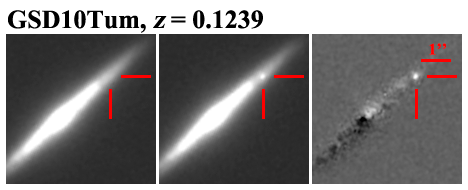
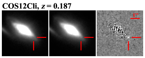
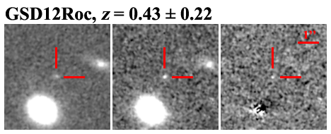
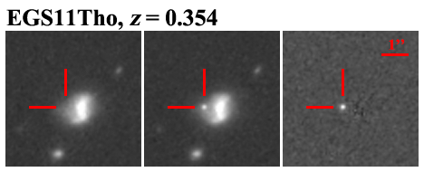
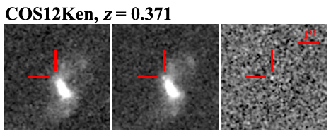
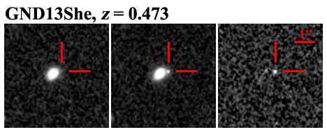
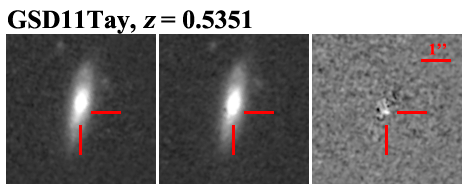
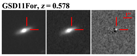
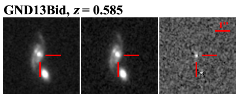
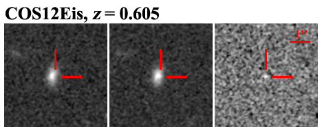
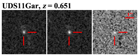
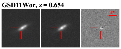
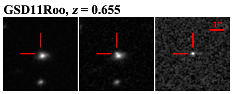
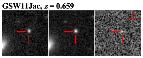
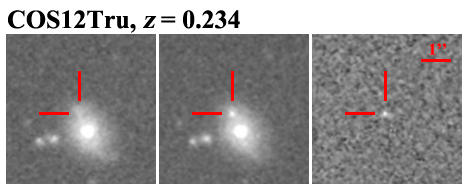
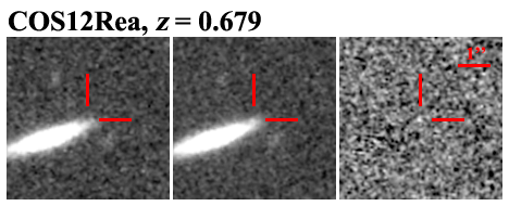
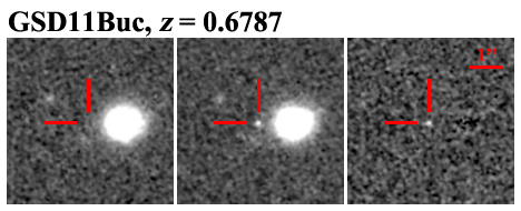
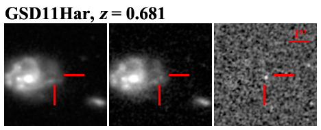
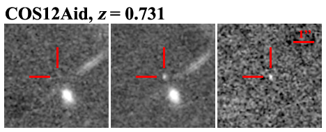
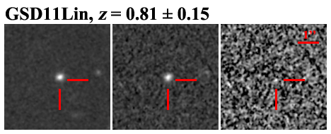
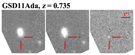
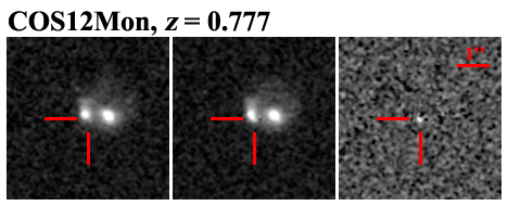
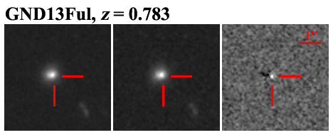
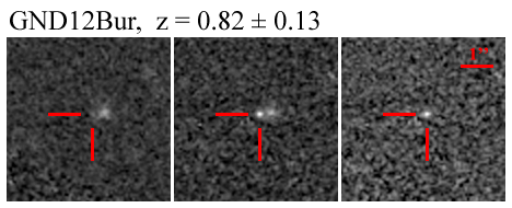
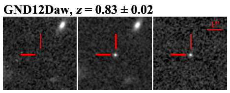
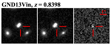
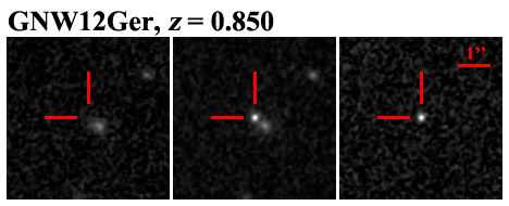
Figure 5.— Detection images for 27 SN from the CANDELS fields with redshifts $z\leq 0.85$. Each image triplet shows H band (F160W) images with the template image on the left, the discovery epoch image in the middle and the difference image on the right. All images have a width of about 6 arcseconds, with North up and East to the left. The position of the SN is marked by (red) crosshairs in every frame.

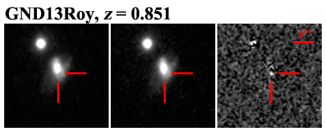
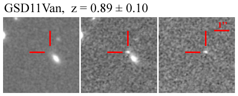
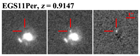
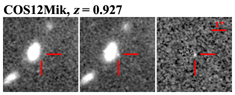
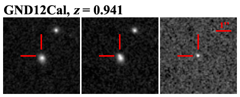
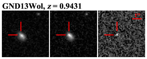
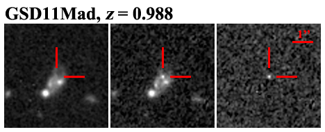
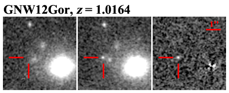
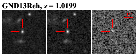
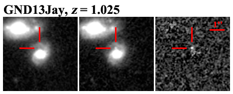
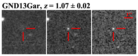
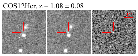
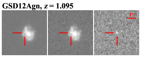
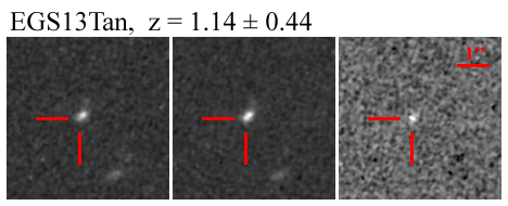
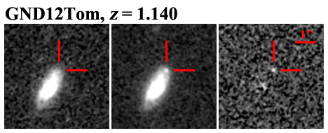
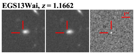
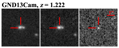
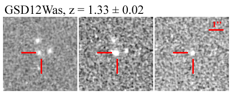
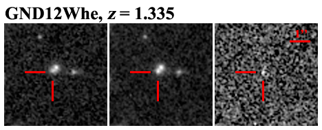
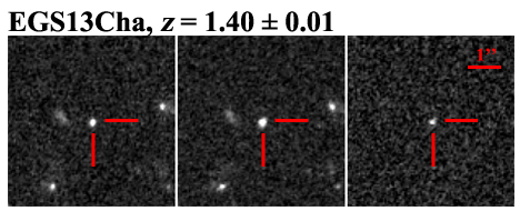
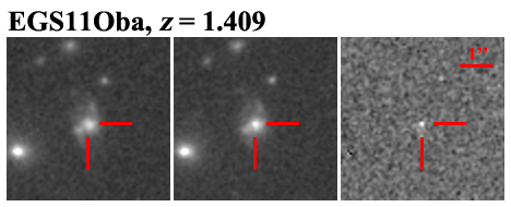
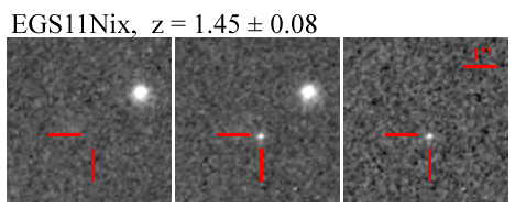
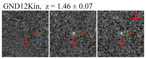
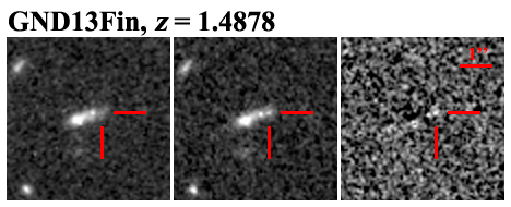
Figure 6.— Detection images for 24 SN from the CANDELS fields with redshifts $0.85<z<1.5$. Each image triplet shows H band (F160W) images with the template image on the left, the discovery epoch image in the middle and the difference image on the right. All images have a width of about 6 arcseconds, with North up and East to the left. The position of the SN is marked by (red) crosshairs in every frame.

Table 951 Supernovae with $z<1.5$

Name	R.A. (J2000)	Decl. (J2000)	P(Ia$|$Dz)	P(Ia$|$Dhost)	z${}_{\mbox{\scriptsize SN}}$	($\pm$)	$z$ Source
GSD10Tum	03:32:17.705	$-$27:50:57.50	0.00 ${}^{+0.00}_{-0.00}$	0.00 ${}^{+0.00}_{-0.00}$	0.124	(0.001)	host spec-z
COS12Cli	10:00:15.958	$+$02:12:36.27	0.29 ${}^{+0.14}_{-0.28}$	0.29 ${}^{+0.03}_{-0.29}$	0.187	(0.001)	host spec-z
GSD12Roc	03:32:06.368	$-$27:47:26.63	0.00 ${}^{+0.00}_{-0.00}$	0.00 ${}^{+0.00}_{-0.00}$	0.346	(0.003)	host spec-z
EGS11Tho	14:19:31.775	$+$52:51:56.16	0.99 ${}^{+0.01}_{-0.98}$	0.99 ${}^{+0.00}_{-0.98}$	0.354	(0.001)	host spec-z
COS12Ken	10:00:36.010	$+$02:15:26.53	0.00 ${}^{+0.00}_{-0.00}$	0.00 ${}^{+0.00}_{-0.00}$	0.373	(0.001)	host spec-z
GND13She	12:36:09.877	$+$62:14:06.00	0.18 ${}^{+0.33}_{-0.18}$	0.31 ${}^{+0.25}_{-0.31}$	0.473	(0.001)	host spec-z
GSD11Tay	03:32:54.505	$-$27:47:04.23	0.67 ${}^{+0.21}_{-0.64}$	0.72 ${}^{+0.12}_{-0.64}$	0.535	(0.001)	host spec-z
GSD11For	03:32:14.300	$-$27:47:13.30	0.41 ${}^{+0.26}_{-0.41}$	0.43 ${}^{+0.13}_{-0.42}$	0.578	(0.001)	host spec-z
GND13Bid	12:36:41.325	$+$62:11:42.21	0.00 ${}^{+0.00}_{-0.00}$	0.00 ${}^{+0.00}_{-0.00}$	0.585	(0.001)	host spec-z
COS12Eis	10:00:47.233	$+$02:11:50.50	0.53 ${}^{+0.14}_{-0.18}$	0.69 ${}^{+0.04}_{-0.01}$	0.605	(0.001)	host spec-z
UDS11Gar	02:17:39.633	$-$05:11:37.14	0.03 ${}^{+0.09}_{-0.03}$	0.08 ${}^{+0.10}_{-0.08}$	0.651	(0.001)	host spec-z
GSD11Wor	03:32:10.739	$-$27:48:07.17	1.00 ${}^{+0.00}_{-0.00}$	1.00 ${}^{+0.00}_{-0.00}$	0.654	(0.001)	host spec-z
GSD11Roo	03:32:31.587	$-$27:46:12.53	0.00 ${}^{+0.00}_{-0.00}$	0.01 ${}^{+0.00}_{-0.00}$	0.655	(0.001)	host spec-z
GSW11Jac	03:32:32.300	$-$27:54:20.55	0.17 ${}^{+0.13}_{-0.11}$	0.18 ${}^{+0.04}_{-0.06}$	0.659	(0.001)	host spec-z
COS12Tru	10:00:38.322	$+$02:11:36.41	0.46 ${}^{+0.32}_{-0.46}$	0.52 ${}^{+0.22}_{-0.52}$	0.665	(0.001)	host spec-z
COS12Rea	10:00:31.917	$+$02:14:16.15	0.00 ${}^{+0.00}_{-0.00}$	0.00 ${}^{+0.00}_{-0.00}$	0.679	(0.001)	host spec-z
GSD11Buc	03:32:28.800	$-$27:52:32.00	0.01 ${}^{+0.01}_{-0.01}$	0.10 ${}^{+0.06}_{-0.10}$	0.679	(0.001)	host spec-z
GSD11Har	03:32:30.441	$-$27:45:18.70	0.32 ${}^{+0.28}_{-0.32}$	0.25 ${}^{+0.12}_{-0.25}$	0.681	(0.001)	host spec-z
COS12Aid	10:00:15.252	$+$02:17:32.12	0.00 ${}^{+0.00}_{-0.00}$	0.00 ${}^{+0.00}_{-0.00}$	0.731	(0.001)	host spec-z
GSD11Lin	03:32:29.812	$-$27:49:19.71	0.00 ${}^{+0.00}_{-0.00}$	0.01 ${}^{+0.00}_{-0.01}$	0.734	(0.001)	host spec-z
GSD11Ada	03:32:19.805	$-$27:54:10.04	0.01 ${}^{+0.02}_{-0.01}$	0.01 ${}^{+0.01}_{-0.01}$	0.735	(0.001)	host spec-z
COS12Mon	10:00:26.737	$+$02:15:13.74	0.02 ${}^{+0.06}_{-0.02}$	0.49 ${}^{+0.19}_{-0.49}$	0.777	(0.001)	host spec-z
GND13Ful	12:36:19.201	$+$62:15:12.58	0.00 ${}^{+0.00}_{-0.00}$	0.00 ${}^{+0.00}_{-0.00}$	0.783	(0.001)	host spec-z
GND12Bur	12:36:32.536	$+$62:15:32.62	0.00 ${}^{+0.00}_{-0.00}$	0.00 ${}^{+0.00}_{-0.00}$	0.82	(0.13)	host+SN phot-z
GND12Daw	12:36:41.340	$+$62:18:52.50	0.00 ${}^{+0.00}_{-0.00}$	0.00 ${}^{+0.00}_{-0.00}$	0.83	(0.02)	SN spec-z + phot-z
GND13Vin	12:37:06.354	$+$62:15:17.79	0.11 ${}^{+0.18}_{-0.11}$	0.13 ${}^{+0.09}_{-0.13}$	0.840	(0.001)	host spec-z
GNW12Ger	12:37:17.023	$+$62:20:38.67	0.05 ${}^{+0.02}_{-0.03}$	0.66 ${}^{+0.00}_{-0.10}$	0.850	(0.001)	host spec-z
GND13Roy	12:36:46.223	$+$62:15:27.13	0.00 ${}^{+0.00}_{-0.00}$	0.00 ${}^{+0.00}_{-0.00}$	0.851	(0.001)	host spec-z
GSD11Van	03:32:19.037	$-$27:47:17.90	0.05 ${}^{+0.12}_{-0.05}$	0.19 ${}^{+0.18}_{-0.19}$	0.886	(0.097)	host+SN phot-z
EGS11Per	14:18:28.318	$+$52:42:45.88	0.99 ${}^{+0.00}_{-0.01}$	1.00 ${}^{+0.00}_{-0.00}$	0.915	(0.001)	host spec-z
COS12Mik	10:00:31.687	$+$02:26:13.73	0.00 ${}^{+0.00}_{-0.00}$	0.01 ${}^{+0.00}_{-0.00}$	0.927	(0.001)	host spec-z
GND12Cal	12:37:10.487	$+$62:15:47.67	1.00 ${}^{+0.00}_{-0.00}$	1.00 ${}^{+0.00}_{-0.00}$	0.941	(0.005)	host spec-z
GND13Wol	12:36:58.946	$+$62:18:10.15	0.31 ${}^{+0.08}_{-0.12}$	0.58 ${}^{+0.02}_{-0.05}$	0.943	(0.001)	host spec-z
GSD11Mad	03:32:18.781	$-$27:52:42.05	1.00 ${}^{+0.00}_{-0.00}$	1.00 ${}^{+0.00}_{-0.00}$	0.988	(0.001)	host spec-z
GNW12Gor	12:36:20.704	$+$62:08:45.08	0.09 ${}^{+0.10}_{-0.08}$	0.23 ${}^{+0.07}_{-0.15}$	1.016	(0.001)	host spec-z
GND13Reh	12:36:54.452	$+$62:11:52.47	0.00 ${}^{+0.00}_{-0.00}$	0.09 ${}^{+0.03}_{-0.06}$	1.019	(0.001)	host spec-z
GND13Jay	12:36:41.380	$+$62:11:30.02	1.00 ${}^{+0.00}_{-0.01}$	1.00 ${}^{+0.00}_{-0.00}$	1.03	(0.01)	host spec-z
GND13Gar	12:36:40.806	$+$62:11:14.16	1.00 ${}^{+0.00}_{-0.00}$	1.00 ${}^{+0.00}_{-0.00}$	1.067	(0.008)	SN spec-z + phot-z
COS12Her	10:00:47.446	$+$02:15:17.74	0.01 ${}^{+0.00}_{-0.00}$	0.02 ${}^{+0.03}_{-0.01}$	1.082	(0.077)	host+SN phot-z
GSD12Agn	03:32:25.902	$-$27:50:19.62	0.80 ${}^{+0.13}_{-0.71}$	0.82 ${}^{+0.07}_{-0.63}$	1.095	(0.001)	host spec-z
EGS13Tan	14:20:02.098	$+$53:00:16.36	0.15 ${}^{+0.05}_{-0.08}$	0.35 ${}^{+0.07}_{-0.07}$	1.137	(0.439)	host+SN phot-z
GND12Tom	12:36:42.543	$+$62:18:21.93	0.86 ${}^{+0.09}_{-0.75}$	0.85 ${}^{+0.06}_{-0.63}$	1.14	(0.001)	host spec-z
EGS13Wai	14:20:28.534	$+$53:04:58.61	1.00 ${}^{+0.00}_{-0.00}$	1.00 ${}^{+0.00}_{-0.00}$	1.166	(0.001)	host spec-z
GND13Cam	12:37:07.354	$+$62:10:26.90	1.00 ${}^{+0.00}_{-0.01}$	1.00 ${}^{+0.00}_{-0.00}$	1.222	(0.002)	host spec-z
GSD11Was	03:32:20.856	$-$27:49:41.48	1.00 ${}^{+0.00}_{-0.00}$	1.00 ${}^{+0.00}_{-0.00}$	1.33	(0.02)	SN spec-z + phot-z
GND12Whe	12:36:24.220	$+$62:17:39.70	0.00 ${}^{+0.00}_{-0.00}$	0.00 ${}^{+0.00}_{-0.00}$	1.335	(0.005)	host spec-z
EGS13Cha	14:20:24.200	$+$53:03:37.50	0.36 ${}^{+0.01}_{-0.14}$	0.80 ${}^{+0.01}_{-0.11}$	1.40	(0.01)	host spec-z
EGS11Oba	14:20:32.663	$+$53:02:48.18	0.91 ${}^{+0.02}_{-0.17}$	0.90 ${}^{+0.00}_{-0.05}$	1.409	(0.001)	host spec-z
EGS11Nix	14:20:48.603	$+$53:00:26.47	0.40 ${}^{+0.01}_{-0.11}$	0.58 ${}^{+0.04}_{-0.10}$	1.451	(0.077)	host+SN phot-z
GND12Kin	12:37:13.005	$+$62:16:30.83	0.00 ${}^{+0.00}_{-0.00}$	0.00 ${}^{+0.00}_{-0.00}$	1.46	(0.07)	host+SN phot-z
GND13Fin	12:37:18.173	$+$62:17:09.65	0.03 ${}^{+0.06}_{-0.03}$	0.02 ${}^{+0.01}_{-0.01}$	1.488	(0.001)	host spec-z

Table 10Host galaxies of 51 Supernovae with $z<1.5$

SN	R.A. (J2000)	Decl. (J2000)	d[′′]	d[kpc]	Morph.	SED	z${}_{\mbox{host}}$	($\pm$)	$z$ Reference
GSD10Tum	03:32:17.871	$-$27:50:59.48	2.96	57.9	d	A	0.124	0.001	Le Fèvre et al. (2004)
COS12Cli	10:00:16.060	$+$02:12:37.38	1.89	37.8	d	SB	0.187	0.001	Trump et al. (2009)
GSD12Roc	03:32:06.368	$-$27:47:26.63	0.00	0.0	i	SB	0.346	0.003	Keck+DEIMOS (B.Mobasher, S.Jha)
EGS11Tho	14:19:31.685	$+$52:51:56.05	0.82	16.8	di	A	0.354	0.001	Keck+LRIS (A. Filippenko), Gemini+GMOS (S. Jha)
COS12Ken	10:00:35.978	$+$02:15:25.81	0.87	17.6	di	SB	0.373	0.001	Lilly et al. (2009)
GND13She	12:36:09.907	$+$62:14:05.79	0.30	6.1	sd	A	0.473	0.001	Wirth et al. (2004)
GSD11Tay	03:32:54.502	$-$27:47:03.67	0.56	11.5	d	A	0.535	0.001	Le Fèvre et al. (2004)
GSD11For	03:32:14.320	$-$27:47:13.15	0.30	6.3	d	A	0.578	0.001	Mignoli et al. (2005)
GND13Bid	12:36:41.417	$+$62:11:42.53	0.72	14.7	i	A	0.585	0.001	Cohen et al. (2000)
COS12Eis	10:00:47.275	$+$02:11:50.04	0.78	15.9	sd	SB	0.605	0.001	Keck+DEIMOS (B.Mobasher)
UDS11Gar	02:17:39.631	$-$05:11:37.00	0.14	3.0	sd	SB	0.651	0.001	Keck+DEIMOS (B.Mobasher)
GSD11Wor	03:32:10.730	$-$27:48:07.14	0.12	2.6	d	A	0.654	0.001	Mignoli et al. (2005)
GSD11Roo	03:32:31.581	$-$27:46:12.71	0.20	4.1	s	SB	0.655	0.001	VLT+FORS2 (B.Leibundgut)
GSW11Jac	03:32:32.310	$-$27:54:20.46	0.16	3.3	d	A	0.659	0.001	VLT+Xshooter (J.Hjorth)
COS12Tru	10:00:38.293	$+$02:11:35.60	0.92	18.7	d	A	0.665	0.001	Keck+DEIMOS (B.Mobasher)
COS12Rea	10:00:32.021	$+$02:14:15.43	1.72	34.4	d	SB	0.679	0.001	Lilly et al. (2009)
GSD11Buc	03:32:28.714	$-$27:52:32.00	1.14	23.1	s	A	0.679	0.001	Le Fèvre et al. (2004)
GSD11Har	03:32:30.570	$-$27:45:18.35	1.75	35.0	d	SB	0.681	0.001	Le Fèvre et al. (2004), Mignoli et al. (2005)
COS12Aid	10:00:15.212	$+$02:17:30.84	1.41	28.5	sd	SB	0.731	0.001	Keck+DEIMOS (B.Mobasher)
GSD11Lin	03:32:29.799	$-$27:49:19.26	0.48	9.9	sd	SB	0.734	0.001	Keck+DEIMOS (A.Filippenko, S.Jha)
GSD11Ada	03:32:19.785	$-$27:54:09.15	0.93	18.9	sd	SB	0.735	0.001	Balestra et al. (2010), Popesso et al. (2009)
COS12Mon	10:00:26.746	$+$02:15:14.02	0.31	6.4	s	SB	0.777	0.001	Lilly et al. (2009)
GND13Ful	12:36:19.227	$+$62:15:12.76	0.26	5.3	sd	SB	0.783	0.001	Wirth et al. (2004)
GND12Bur	12:36:32.464	$+$62:15:32.75	0.52	10.7	i	SB	0.69	0.4	phot-z (T.Dahlen)
GND12Daw	$\cdots$	$\cdots$	$\cdots$	$\cdots$	$\cdots$	$\cdots$	$\cdots$	$\cdots$	$\cdots$
GND13Vin	12:37:06.308	$+$62:15:18.08	0.43	8.9	i	A	0.840	0.001	Cohen et al. (2000)
GNW12Ger	12:37:16.965	$+$62:20:38.34	0.52	10.7	s	A	0.850	0.005	Keck+DEIMOS (A.Filippenko)
GND13Roy	12:36:46.232	$+$62:15:27.46	0.34	6.9	i	SB	0.851	0.001	Cooper et al. (2011)
GSD11Van	03:32:19.004	$-$27:47:18.33	0.61	12.6	d	P	0.74	0.15	phot-z (T.Dahlen)
EGS11Per	14:18:28.248	$+$52:42:45.07	1.03	20.9	d	A	0.915	0.001	Barro et al. (2011)
COS12Mik	10:00:31.733	$+$02:26:13.92	0.72	14.6	sd	SB	0.927	0.001	Keck+DEIMOS (B.Mobasher)
GND12Cal	12:37:10.476	$+$62:15:47.40	0.28	5.8	s	SB	0.941	0.005	HST+WFC3 (B.Weiner)
GND13Wol	12:36:58.933	$+$62:18:10.04	0.14	3.0	sd	SB	0.9431	0.0002	Barger et al. (2008)
GSD11Mad	03:32:18.767	$-$27:52:42.45	0.44	9.1	d	SB	0.988	0.001	Keck+LRIS (A.Filippenko)
GNW12Gor	12:36:20.619	$+$62:08:44.91	0.62	12.7	u	A	1.0164	0.0005	Wirth et al. (2004), Treu et al. (2005)
GND13Reh	12:36:54.445	$+$62:11:52.43	0.06	1.3	s	SB	1.019	0.001	Barger et al. (2008)
GND13Jay	12:36:41.370	$+$62:11:29.57	0.46	9.4	d	A	1.03	0.01	HST+WFC3 (B.Weiner)
GND13Gar	12:36:40.813	$+$62:11:14.34	0.19	3.9	u	SB	1.07	0.02	phot-z (T.Dahlen)
COS12Her	10:00:47.438	$+$02:15:17.35	0.41	8.4	s	SB	1.1	0.4	Keck+DEIMOS (B.Mobasher)
GSD12Agn	03:32:25.861	$-$27:50:19.81	0.58	11.8	d	SB	1.095	0.001	Vanzella et al. (2008)
EGS13Tan	14:20:02.010	$+$53:00:17.04	1.05	21.3	sd	A	1.39	0.8	phot-z (T.Dahlen)
GND12Tom	12:36:42.636	$+$62:18:20.74	1.36	27.4	d	A	1.140	0.001	Barger et al. (2008)
EGS13Wai	14:20:28.495	$+$53:04:58.72	0.37	7.6	di	SB	1.1662	0.0004	Barro et al. (2011)
GND13Cam	12:37:07.357	$+$62:10:26.94	0.05	0.9	sd	SB	1.222	0.002	HST+WFC3 (B.Weiner)
GSD11Was	03:32:20.856	$-$27:49:41.48	0.00	0.0	d	SB	1.30	0.05	HST+WFC3 (A.Riess)
GND12Whe	12:36:24.206	$+$62:17:39.92	0.24	5.0	sd	SB	1.335	0.001	Keck+DEIMOS (C.Papovich)
EGS13Cha	14:20:24.200	$+$53:03:37.50	0.00	0.0	sd	A	1.40	0.05	Keck+MOSFIRE (M.Cooper)
EGS11Oba	14:20:32.666	$+$53:02:48.10	0.08	1.8	di	A	1.409	0.001	Keck+LRIS (A.Filippenko)
EGS11Nix	14:20:48.607	$+$53:00:26.56	0.10	2.0	u	A	1.73	0.51	phot-z (T.Dahlen)
GND12Kin	12:37:13.013	$+$62:16:30.86	0.06	1.3	u	SB	1.9	0.4	phot-z (T.Dahlen)
GND13Fin	12:37:18.322	$+$62:17:09.34	1.08	22.0	i	SB	1.4878	0.0005	Wirth et al. (2004), Reddy et al. (2006)

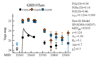
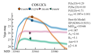
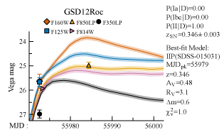
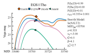
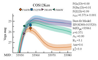
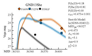
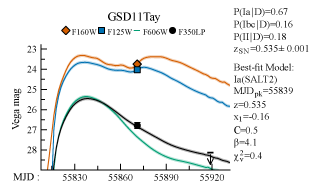
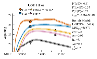
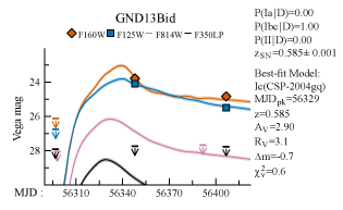
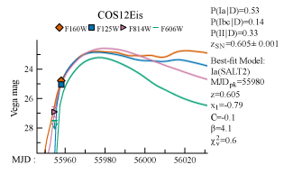
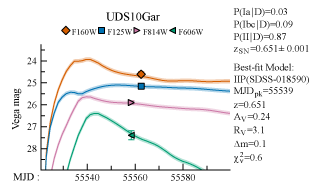
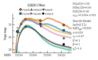
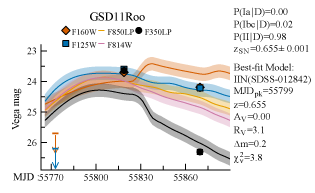
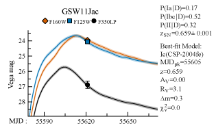
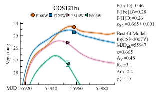
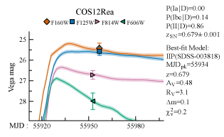
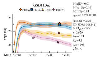
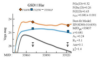
Figure 7.— STARDUST light curve matches for the first 18 SN from the CANDELS fields in redshift order, with redshifts $z<0.7$, as in Figure 2.

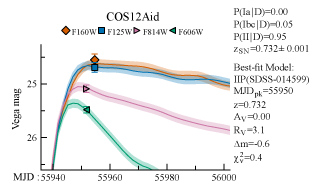
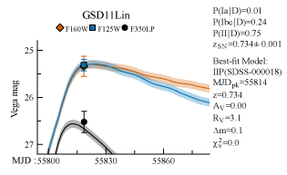
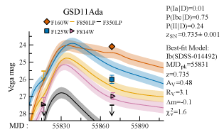
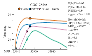
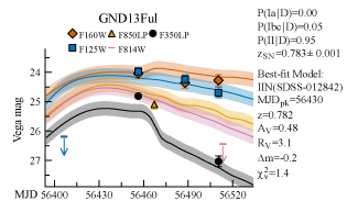
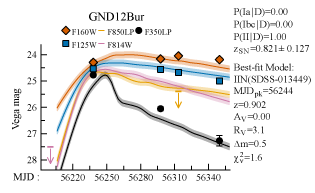
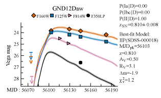
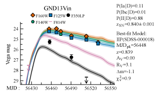
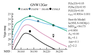
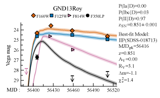
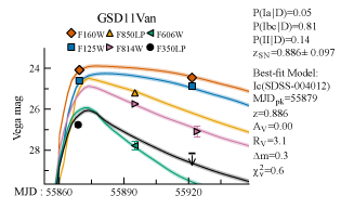
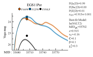
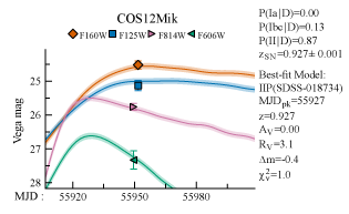
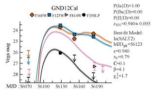
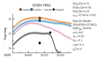
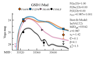
Figure 8.— STARDUST light curve matches for the 16 SN from the CANDELS fields with redshifts $0.7<z<1.0$, as in Figure 2.

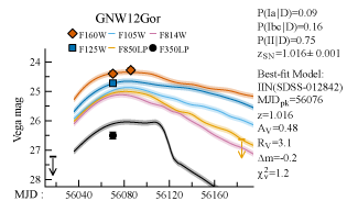
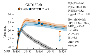
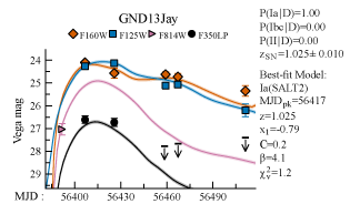
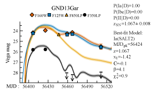
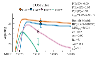
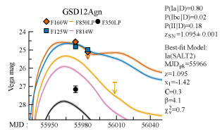
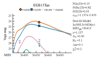
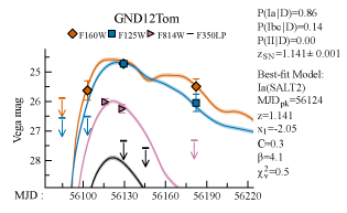
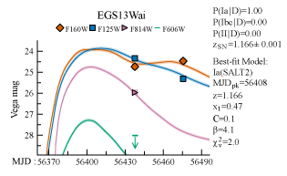
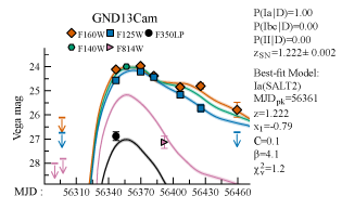
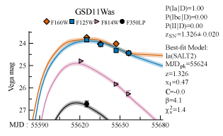
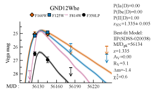
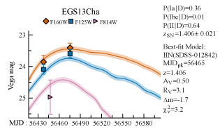
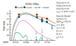
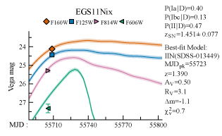
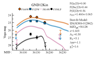
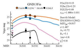
Figure 9.— STARDUST light curve matches for the 17 SN from the CANDELS fields with redshifts $1.0<z<1.5$, as in Figure 2.

References

- Alard & Lupton (1998) Alard, C., & Lupton, R. H. 1998, ApJ, 503, 325
- Astier et al. (2006) Astier, P., Guy, J., Regnault, N., et al. 2006, A&A, 447, 31
- Astropy Collaboration et al. (2013) Astropy Collaboration, Robitaille, T. P., Tollerud, E. J., et al. 2013, A&A, 558, A33
- Balestra et al. (2010) Balestra, I., Mainieri, V., Popesso, P., et al. 2010, A&A, 512, A12
- Barbary et al. (2012) Barbary, K., Aldering, G., Amanullah, R., et al. 2012, ApJ, 745, 31
- Barger et al. (2008) Barger, A. J., Cowie, L. L., & Wang, W.-H. 2008, ApJ, 689, 687
- Barro et al. (2011) Barro, G., Pérez-González, P. G., Gallego, J., et al. 2011, ApJS, 193, 13
- Behroozi et al. (2013) Behroozi, P. S., Wechsler, R. H., & Conroy, C. 2013, ApJ, 770, 57
- Belczynski et al. (2005) Belczynski, K., Bulik, T., & Ruiter, A. J. 2005, ApJ, 629, 915
- Bildsten et al. (2007) Bildsten, L., Shen, K. J., Weinberg, N. N., & Nelemans, G. 2007, ApJ, 662, L95
- Blanc et al. (2004) Blanc, G., Afonso, C., Alard, C., et al. 2004, A&A, 423, 881
- Blondin & Tonry (2007) Blondin, S., & Tonry, J. L. 2007, ApJ, 666, 1024
- Botticella et al. (2008) Botticella, M. T., Riello, M., Cappellaro, E., et al. 2008, A&A, 479, 49
- Bours et al. (2013) Bours, M. C. P., Toonen, S., & Nelemans, G. 2013, A&A, 552, A24
- Cappellaro et al. (1999) Cappellaro, E., Evans, R., & Turatto, M. 1999, A&A, 351, 459
- Chabrier (2003) Chabrier, G. 2003, PASP, 115, 763
- Cirasuolo et al. (2007) Cirasuolo, M., McLure, R. J., Dunlop, J. S., et al. 2007, MNRAS, 380, 585
- Claeys et al. (2014) Claeys, J. S. W., Pols, O. R., Izzard, R. G., Vink, J., & Verbunt, F. W. M. 2014, A&A, 563, A83
- Cohen et al. (2000) Cohen, J. G., Hogg, D. W., Blandford, R., et al. 2000, ApJ, 538, 29
- Cooper et al. (2011) Cooper, M. C., Aird, J. A., Coil, A. L., et al. 2011, ApJS, 193, 14
- Dahlen et al. (2008) Dahlen, T., Strolger, L.-G., & Riess, A. G. 2008, ApJ, 681, 462
- Dahlen et al. (2012) Dahlen, T., Strolger, L.-G., Riess, A. G., et al. 2012, ApJ, 757, 70
- Dahlen et al. (2004) Dahlen, T., Strolger, L.-G., Riess, A. G., et al. 2004, ApJ, 613, 189
- Dahlen et al. (2010) Dahlen, T., Mobasher, B., Dickinson, M., et al. 2010, ApJ, 724, 425
- Dahlen et al. (2013) Dahlen, T., Mobasher, B., Faber, S. M., et al. 2013, ApJ, 775, 93
- D’Andrea et al. (2010) D’Andrea, C. B., Sako, M., Dilday, B., et al. 2010, ApJ, 708, 661
- Davis et al. (2007) Davis, M., Guhathakurta, P., Konidaris, N. P., et al. 2007, ApJ, 660, L1
- Dilday et al. (2010) Dilday, B., Smith, M., Bassett, B., et al. 2010, ApJ, 713, 1026
- Drout et al. (2011) Drout, M. R., Soderberg, A. M., Gal-Yam, A., et al. 2011, ApJ, 741, 97
- Foley & Mandel (2013) Foley, R. J., & Mandel, K. 2013, ApJ, 778, 167
- Foley et al. (2013) Foley, R. J., Challis, P. J., Chornock, R., et al. 2013, ApJ, 767, 57
- Frederiksen et al. (2012) Frederiksen, T. F., Hjorth, J., Maund, J. R., et al. 2012, ApJ, 760, 125
- Frieman et al. (2008) Frieman, J. A., Turner, M. S., & Huterer, D. 2008, ARA&A, 46, 385
- Fruchter & Hook (2002) Fruchter, A. S., & Hook, R. N. 2002, PASP, 114, 144
- Gal-Yam (2012) Gal-Yam, A. 2012, Science, 337, 927
- Giavalisco et al. (2004) Giavalisco, M., Ferguson, H. C., Koekemoer, A. M., et al. 2004, ApJ, 600, L93
- Graur & Maoz (2013) Graur, O., & Maoz, D. 2013, MNRAS, 430, 1746
- Graur et al. (2011) Graur, O., Poznanski, D., Maoz, D., et al. 2011, MNRAS, 417, 916
- Graur et al. (2014) Graur, O., Rodney, S. A., Maoz, D., et al. 2014, ApJ, 783, 28
- Greggio (2010) Greggio, L. 2010, MNRAS, 406, 22
- Grogin et al. (2011) Grogin, N. A., Kocevski, D. D., Faber, S. M., et al. 2011, ApJS, 197, 35
- Guy et al. (2010) Guy, J., Sullivan, M., Conley, A., et al. 2010, A&A, 523, A7
- Hachisu et al. (1996) Hachisu, I., Kato, M., & Nomoto, K. 1996, ApJ, 470, L97+
- Hachisu et al. (1999) —. 1999, ApJ, 522, 487
- Hamuy et al. (2006) Hamuy, M., Folatelli, G., Morrell, N. I., et al. 2006, PASP, 118, 2
- Hardin et al. (2000) Hardin, D., Afonso, C., Alard, C., et al. 2000, A&A, 362, 419
- Hillebrandt & Niemeyer (2000) Hillebrandt, W., & Niemeyer, J. 2000, ARA&A, 38, 191
- Horesh et al. (2008) Horesh, A., Poznanski, D., Ofek, E. O., & Maoz, D. 2008, MNRAS, 389, 1871
- Iben & Tutukov (1984) Iben, Jr., I., & Tutukov, A. V. 1984, ApJS, 54, 335
- Jones et al. (2013) Jones, D. O., Rodney, S. A., Riess, A. G., et al. 2013, ApJ, 768, 166
- Kashi & Soker (2011) Kashi, A., & Soker, N. 2011, MNRAS, 417, 1466
- Kelly et al. (2008) Kelly, P. L., Kirshner, R. P., & Pahre, M. 2008, ApJ, 687, 1201
- Kessler et al. (2009a) Kessler, R., Becker, A. C., Cinabro, D., et al. 2009a, ApJS, 185, 32
- Kessler et al. (2009b) Kessler, R., Bernstein, J. P., Cinabro, D., et al. 2009b, PASP, 121, 1028
- Kiewe et al. (2012) Kiewe, M., Gal-Yam, A., Arcavi, I., et al. 2012, ApJ, 744, 10
- Kobayashi & Nomoto (2009) Kobayashi, C., & Nomoto, K. 2009, ApJ, 707, 1466
- Kobayashi et al. (1998) Kobayashi, C., Tsujimoto, T., Nomoto, K., Hachisu, I., & Kato, M. 1998, ApJ, 503, 155
- Koekemoer et al. (2002) Koekemoer, A. M., Fruchter, A. S., Hook, R. N., & Hack, W. 2002, in The 2002 HST Calibration Workshop, ed. S. Arribas, A. Koekemoer, & B. Whitmore, 337
- Koekemoer et al. (2007) Koekemoer, A. M., Aussel, H., Calzetti, D., et al. 2007, ApJS, 172, 196
- Koekemoer et al. (2011) Koekemoer, A. M., Faber, S. M., Ferguson, H. C., et al. 2011, ApJS, 197, 36
- Krist et al. (2011) Krist, J. E., Hook, R. N., & Stoehr, F. 2011, in SPIE Conference Series, Vol. 8127
- Kuznetsova et al. (2008) Kuznetsova, N., Barbary, K., Connolly, B., et al. 2008, ApJ, 673, 981
- Lawrence et al. (2007) Lawrence, A., Warren, S. J., Almaini, O., et al. 2007, MNRAS, 379, 1599
- Le Fèvre et al. (2004) Le Fèvre, O., Vettolani, G., Paltani, S., et al. 2004, A&A, 428, 1043
- Leaman et al. (2011) Leaman, J., Li, W., Chornock, R., & Filippenko, A. V. 2011, MNRAS, 412, 1419
- Li et al. (2011) Li, W., Leaman, J., Chornock, R., et al. 2011, MNRAS, 412, 1441
- Lilly et al. (2009) Lilly, S. J., Le Brun, V., Maier, C., et al. 2009, ApJS, 184, 218
- Livio (2001) Livio, M. 2001, in SNe and GRBs, ed. M. Livio, N. Panagia, & K. Sahu, 334
- Madau et al. (1998) Madau, P., della Valle, M., & Panagia, N. 1998, MNRAS, 297, L17
- Mannucci et al. (2006) Mannucci, F., Della Valle, M., & Panagia, N. 2006, MNRAS, 370, 773
- Mannucci et al. (2007) Mannucci, F., Della Valle, M., & Panagia, N. 2007, MNRAS, 377, 1229
- Mannucci et al. (2005) Mannucci, F., Della Valle, M., Panagia, N., et al. 2005, A&A, 433, 807
- Maoz & Badenes (2010) Maoz, D., & Badenes, C. 2010, MNRAS, 407, 1314
- Maoz & Mannucci (2012) Maoz, D., & Mannucci, F. 2012, PASA, 29, 447
- Mattila et al. (2012) Mattila, S., Dahlen, T., Efstathiou, A., et al. 2012, ApJ, 756, 111
- Melinder et al. (2012) Melinder, J., Dahlen, T., Mencía Trinchant, L., et al. 2012, A&A, 545, A96
- Mennekens et al. (2010) Mennekens, N., Vanbeveren, D., De Greve, J. P., & De Donder, E. 2010, A&A, 515, A89+
- Mennekens et al. (2013) Mennekens, N., Vanbeveren, D., De Greve, J.-P., & De Donder, E. 2013, in IAU Symposium, Vol. 281, IAU Symposium, ed. R. Di Stefano, M. Orio, & M. Moe, 232–235
- Mignoli et al. (2005) Mignoli, M., Cimatti, A., Zamorani, G., et al. 2005, A&A, 437, 883
- Morrell (2012) Morrell, N. I. 2012, in IAU Symposium, Vol. 279, Death of Massive Stars: Supernovae and Gamma-Ray Bursts, 361
- Murphy et al. (2009) Murphy, E. J., Chary, R.-R., Alexander, D. M., et al. 2009, ApJ, 698, 1380
- Neill et al. (2006) Neill, J. D., Sullivan, M., Balam, D., et al. 2006, AJ, 132, 1126
- Pain et al. (2002) Pain, R., Fabbro, S., Sullivan, M., et al. 2002, ApJ, 577, 120
- Paterno (2004) Paterno, M. 2004, FERMILAB-TM-2286-CD
- Perrett et al. (2012) Perrett, K., Sullivan, M., Conley, A., et al. 2012, AJ, 144, 59
- Popesso et al. (2009) Popesso, P., Dickinson, M., Nonino, M., et al. 2009, A&A, 494, 443
- Postman et al. (2012) Postman, M., Coe, D., Benítez, N., et al. 2012, ApJS, 199, 25
- Poznanski et al. (2007) Poznanski, D., Maoz, D., Yasuda, N., et al. 2007, MNRAS, 382, 1169
- Quimby et al. (2011) Quimby, R. M., Kulkarni, S. R., Kasliwal, M. M., et al. 2011, Nature, 474, 487
- Raskin et al. (2009) Raskin, C., Scannapieco, E., Rhoads, J., & Della Valle, M. 2009, ApJ, 707, 74
- Reddy et al. (2006) Reddy, N. A., Steidel, C. C., Erb, D. K., Shapley, A. E., & Pettini, M. 2006, ApJ, 653, 1004
- Riess et al. (2007) Riess, A. G., Strolger, L.-G., Casertano, S., et al. 2007, ApJ, 659, 98
- Rodney & Tonry (2010) Rodney, S. A., & Tonry, J. L. 2010, ApJ, 723, 47
- Rodney et al. (2012) Rodney, S. A., Riess, A. G., Dahlen, T., et al. 2012, ApJ, 746, 5
- Ruiter et al. (2009) Ruiter, A. J., Belczynski, K., & Fryer, C. 2009, ApJ, 699, 2026
- Ruiter et al. (2013) Ruiter, A. J., Sim, S. A., Pakmor, R., et al. 2013, MNRAS, 429, 1425
- Sako et al. (2008) Sako, M., Bassett, B., Becker, A., et al. 2008, AJ, 135, 348
- Scannapieco & Bildsten (2005) Scannapieco, E., & Bildsten, L. 2005, ApJ, 629, L85
- Scoville et al. (2007) Scoville, N., Aussel, H., Brusa, M., et al. 2007, ApJS, 172, 1
- Sharon et al. (2007) Sharon, K., Gal-Yam, A., Maoz, D., Filippenko, A. V., & Guhathakurta, P. 2007, ApJ, 660, 1165
- Smartt et al. (2009) Smartt, S. J., Eldridge, J. J., Crockett, R. M., & Maund, J. R. 2009, MNRAS, 395, 1409
- Stritzinger et al. (2009) Stritzinger, M., Mazzali, P., Phillips, M. M., et al. 2009, ApJ, 696, 713
- Strolger et al. (2010) Strolger, L., Dahlen, T., & Riess, A. G. 2010, ApJ, 713, 32
- Strolger et al. (2004) Strolger, L.-G., Riess, A. G., Dahlen, T., et al. 2004, ApJ, 613, 200
- Thompson (2011) Thompson, T. A. 2011, ApJ, 741, 82
- Tonry et al. (2003) Tonry, J. L., Schmidt, B. P., Barris, B., et al. 2003, ApJ, 594, 1
- Treu et al. (2005) Treu, T., Ellis, R. S., Liao, T. X., & van Dokkum, P. G. 2005, ApJ, 622, L5
- Trump et al. (2009) Trump, J. R., Impey, C. D., Elvis, M., et al. 2009, ApJ, 696, 1195
- Vanzella et al. (2008) Vanzella, E., Cristiani, S., Dickinson, M., et al. 2008, A&A, 478, 83
- Wang et al. (2009) Wang, B., Chen, X., Meng, X., & Han, Z. 2009, ApJ, 701, 1540
- Webbink (1984) Webbink, R. F. 1984, ApJ, 277, 355
- Whelan & Iben (1973) Whelan, J., & Iben, I. J. 1973, ApJ, 186, 1007
- Wiersma et al. (2011) Wiersma, R. P. C., Schaye, J., & Theuns, T. 2011, MNRAS, 415, 353
- Wirth et al. (2004) Wirth, G. D., Willmer, C. N. A., Amico, P., et al. 2004, AJ, 127, 3121