The value of in the inhomogeneous Universe
Abstract
Local measurements of the Hubble expansion rate are affected by structures like galaxy clusters or voids. Here we present a fully relativistic treatment of this effect, studying how clustering modifies the mean distance (modulus)-redshift relation and its dispersion in a standard CDM universe. The best estimates of the local expansion rate stem from supernova observations at small redshifts (). It is interesting to compare these local measurements with global fits to data from cosmic microwave background anisotropies. In particular, we argue that cosmic variance (i.e. the effects of the local structure) is of the same order of magnitude as the current observational errors and must be taken into account in local measurements of the Hubble expansion rate.
pacs:
98.80.-k, 95.36.+x, 98.80.EsThe Hubble constant, , determines the present expansion rate of the Universe. For most cosmological phenomena a precise knowledge of is of utmost importance. In a perfectly homogeneous and isotropic world is defined globally. But the Universe contains structures like galaxy clusters and voids. Thus the local expansion rate, measured by means of cepheids and supernovae at small redshifts, does not necessarily agree with the expansion rate of an isotropic and homogeneous model that is used to describe the Universe at the largest scales.
Recent local measurements of the Hubble rate Riess ; Freedman:2012ny are claimed to be accurate at the few percent level, e.g. Riess finds . In the near future, observational techniques will improve further, such that the local value of will be determined at 1% accuracy future , competitive with the current precision of indirect measurements of the global via the cosmic microwave backgound anisotropies Planck .
The observed distance modulus is related to the bolometric flux and the luminosity distance by ()
| (1) |
The relation between the intrinsic luminosity, , the bolometric flux, , and the luminosity distance of a source is . In a flat CDM universe with present matter density parameter the luminosity distance as a function of redshift is given by
| (2) |
As long as we consider only small redshifts, , the dependence on cosmology is weak, and the result varies by about 0.2% when varies within the error bars determined by Planck Planck . However, neglecting the model dependent quadratic term induces an error of nearly 8% for .
The observed Universe is inhomogeneous and anisotropic on small scales and the local Hubble rate is expected to differ from its global value for two reasons. First, any supernova (SN) sample is finite (sample variance) and, second, we observe only one realization of a random configuration of the local structure (cosmic variance). Thus, even for arbitrarily precise measurements of fluxes and redshifts, the local differs from the global . Sample variance is fully taken into account in the literature, but cosmic variance is usually not considered.
In the context of Newtonian cosmology, cosmic variance of the local has been estimated in Shi:1997aa ; Wang:1997tp ; Buchert:1999pq ; Wojtak:2013gda . First attempts to estimate cosmic variance of the local Hubble rate in a relativistic approach can be found in Li:2007ny ; Wiegand:2011je (see also ClarksonetAll ), based on the ensemble variance of the expansion rate averaged over a spatial volume. It has been shown that this approach agrees very well with the Newtonian one Li:2007ny and it predicts a cosmic variance which depends on the sampling volume on the sub-per cent to per cent level. However, this approach still neglects the fact that observers probe the past light-cone and not a spatial volume. Also, the measured quantity is not an expansion rate, but a set of the bolometric fluxes and redshifts.
In this letter, we present the first fully relativistic estimation of the effects of clustering on the local measurement of the Hubble parameter without making any special hypothesis about how the fluctuations can be modeled around us. Considering only the measured quantities and the cosmological standard model with stochastic inhomogeneities, we study the effect of cosmic structures on the local determination of , i.e., taking light propagation effects fully into account. Other relativistic approaches were recently proposed in FDU ; Marra:2013rba . In FDU a ”Swiss cheese” model was used in modeling the local Universe, in Marra:2013rba a “Hubble bubble” model was used and the perturbation of the expansion rate, which is not directly measurable, was considered.
We shall find that the mean value of the Hubble parameter is modified at sub-percent level, while the contribution from clustering to the error budget is larger, typically to , hence as large as observational errors quoted in the literature Riess . As we shall see, the small modification of the mean of the Hubble parameter can be reduced by a factor of by using the flux instead of the distance modulus. On the other hand, the cosmic variance induced by inhomogeneities on is independent of the observable used. Finally, we find that even for an infinite number of SNIa within with identical redshift distribution compared to a finite sample considered, clustering induces a minimal error of about for a local determination of .
Following BGMNVprl ; BGMNVfeb2013 we use cosmological perturbation theory up to second order with an almost scale-invariant initial power spectrum to determine the mean perturbation of the bolometric flux (and of the distance modulus) from a standard candle and its variance.
Let us first consider the fluctuation of the mean on a sphere at fixed observed redshift . We denote the light-cone average GMNV over a surface at fixed redshift by , and a statistical average by . Using the results of BMNG ; FGMV (see also BDG ) the fluctuation of the flux , away from its background value in the Friedmann-Lemaître Universe (denoted by ), is given by
| (3) |
where we expand up to second order in perturbation theory. The ensemble average of vanishes at first order, but not at second order and must be added to another second order contribution from ; we obtain (see, e.g. BGMNV1 )
| (4) |
where for
| (5) |
Here denotes the direction to a given SN and its peculiar velocity, is conformal time, is the difference between the present time and the time at redshift , and is the conformal Hubble parameter. In BGMNVfeb2013 the full contribution is given in terms of 39 Fourier integrals over the dimensionless power spectrum of the Bardeen potential today, with different kernels. We have removed the observer velocity since observations are usually quoted in the CMB frame, corresponding to . A non-vanishing observer velocity would nearly double the effect in Eq. (5). The dominant peculiar velocity contribution at low redshift gives
| (6) |
where
is the growth factor and the source and the observer times are indicated with the suffix and .
The brightness of supernovae is typically expressed in terms of the distance modulus . Due to the nonlinear function relating and one obtains different second order contributions,
| (7) |
where, at , we also find
| (8) |
The approximate equalities in Eqs. (5) and (8) are valid for , where the first order squared contribution of the peculiar velocity terms dominates over the other second order contributions. For and larger, additional contributions notably due to lensing become relevant, see BGMNVprl ; BGMNVfeb2013 .
For measurements of the Hubble parameter, low redshift SNe are used in order to minimize the dependence of the result on cosmological parameters. As a consequence, Eqs. (5) and (8) are good approximations for the aim of this Letter.
Hereafter we use the cosmological parameters from Planck Planck , the linear transfer function given in EH taking baryons into account, and , see BGMNVfeb2013 for details. Increasing the cut-off does not change our result due to two effects: the kernel of the peculiar velocity contribution decreases at large and small scale fluctuations are incoherent (see below) and their contribution to the variance decays like , where is the number of supernovae.
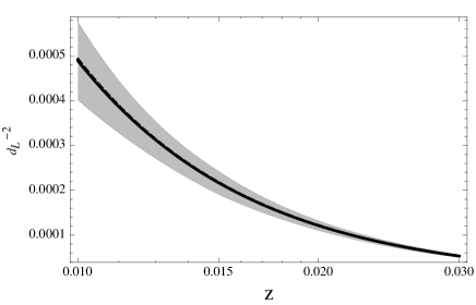
As an illustration for the effects of cosmic structure on the observed flux from SN, we plot in Fig. 1 the average and its variance (as defined in BGMNV1 ), using Eqs. (4-6) and (8). Figure 1 clearly shows how at low redshift the dispersion of the flux is much more important than the shift of the average (see also BGMNVprl ; BGMNVfeb2013 ).
Comparing Eqs. (4) and (7), we see that the flux averaged over a sphere at constant redshift, experiences a different effect than the distance modulus averaged over the same sphere.
On the other hand, the induced theoretical dispersion on the bare value of , which is entirely due to squared first order perturbations, is independent of the observable considered to infer . To determine the dispersion of from a sample of SNe we consider that at small redshift . inferred from the observation of a single SN at redshift , is then expected to deviate from the true by approximately BGMNV1
| (9) |
Of course in practice, observers do not have at their disposal many SNe at the same redshift, so the average over a sphere cannot be performed. Hence, we now go beyond this simplifying assumption of previous works.
Let us estimate the (ensemble) variance of the locally measured Hubble parameter from the covariance matrix of the fluxes, given an arbitrarily distributed sample of observed SNe at positions , which reads
| (10) | |||||
with
| (11) |
and
| (12) | |||||
where and . Here is the comoving distance between the SNe at and , denotes the spherical Bessel function of order and is the unit vector in direction . To arrive at (12), we have introduced the Fourier representation of and used some well known identities. Note that with and Eqs.(6) and (8), the auto-correlation term reproduces (9).
If the fluxes are perfectly coherent for all SNe so that , for all correlations, we obtain , while in the incoherent case, we obtain . The reality lies somewhere in-between, wavelengths with being rather coherent while those with are rather incoherent.
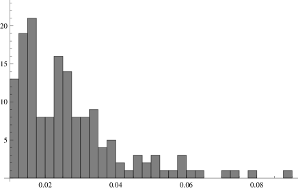
In order to estimate the effect of the cosmic (co)variance for a realistic sample of SNe, we consider the following set up. We calculate from Eqs. (10) to (12) considering the redshifts of a sample of 155 SNe selected to lie in the range from the CfA3 and OLD samples Hicken ; Jha:2006fm . The redshift distribution of the sample is shown in Fig 2. We do not use their actual positions on the sky (see below). We then also study the limiting case of infinitely many SNe.
For the redshift distribution of the 155 SNe of this sample, Eq. (10) yields a dispersion induced by inhomogeneities between and for different angular distributions for the SNe. From this range we infer
| (13) |
with as given in Riess (where ”……” stands for ”from…to…”). We have kept constant to different values and we have chosen a random distribution of directions over one hemisphere. The different choices give rise to the range quoted above. The smallest error corresponds to a random distribution of directions over one hemisphere, while the largest one corresponds to the case where all SNe are inside a narrow cone (). The dispersion due to the actual angular distribution of real SN samples is left for future studies.
Let us also estimate the effect of inhomogeneities on the measured value of itself for this sample. In Riess a partial reconstruction of the peculiar velocity field has been applied, which however comes from the density field in the neighborhood of the SNe and therefore contributes only an incoherent part which we neglect. Considering a perfectly homogeneous Universe, a measured Hubble parameter is deduced from the measurement of with a constant, see Eqs. (1,2). However this is not the true underlying , since it ignores the local large-scale structure, and therefore gives a biased value. The true underlying Hubble parameter is derived only by applying the appropriate correction due to this structure. Comparing Eq. (7) with the above expression, we have:
| (14) |
We now consider the 155 SNe of the sample used here and generate the mean value of the corrected , starting from a value of and for the given redshift distribution. The final result is about higher than 111Choosing a larger cut-off affects only this result slightly.. A similar global shift has already been included in the analysis of Riess as a consequence of the partial reconstruction of the peculiar velocity field Riess1 . Let us underline that the correction to would be three times smaller if we would consider the backreaction on the flux instead of the one on the distance modulus. In this case Eq. (14) should be replaced by .
Considering the quoted observational error of 2.4 km/s/Mpc Riess and the additional variance (13), we obtain
| (15) |
The tension with the Planck measurement Planck , for which a value is reported, is reduced when taking this additional variance into account. In particular, adding the above errors in quadrature we obtain a deviation of to from , while the difference is when using the error quoted in Riess . This analysis is insensitive to smaller scales fluctuations due to the incoherence of such contributions. Further modeling of these scales, e.g. FDU (see also Fleury:2014gha ), might increase the uncertainty. However, effects from nearby small-scale structure are at least partly included in the analysis of Riess .
Before concluding, we want to determine the ultimate error for an arbitrarily large sample when the SNe are distributed isotropically over directions. In this case we can integrate over all directions. With
we obtain, for a normalized redshift distribution ,
| (16) |
with . Approximating the redshift distribution of our sample using an interpolating function of the histogram in Fig 2, integrating from to , we obtain a dispersion of about which corresponds to an error of
| (17) |
This is the minimal dispersion of a SN sample with a redshift space distribution given by the one in Fig 2. It is not much smaller than the value obtained for the real sample. Interestingly, this result is close to the ones obtained in Li:2007ny ; Marra:2013rba ; Wojtak:2013gda , some of them with a very different analysis.
The errors from the nearby SNe with small give the largest contribution. Therefore, the dispersion can be reduced by considering higher redshift SNe for which, however, the model dependence becomes more relevant. If we consider higher redshifts (close to or larger than ), we have to take into account also the other contributions to the perturbation of the luminosity distance, see BMNG ; FGMV ; BDG for the full expression. As it is well known (see, for example, BGMNVprl ; BGMNVfeb2013 ), at redshift , the lensing term begins to dominate.
In Neill the peculiar velocity field has been reconstructed using the IRAS PSCz catalog Branchini . As already mentioned above, this is subtracted in the analysis of Riess . It is clear that this procedure also modifies the expected mean and its variance in our method, but a detailed analysis of this is beyond the scope of this work. As the (minimal) cosmic variance Eq. (17) receives mainly contributions from scales larger than those considered in the reconstruction, we expect that it still has to be taken into account, in addition to the reconstructed peculiar velocities.
To conclude, in this Letter we estimate the impact of stochastic inhomogeneities on the local value of the Hubble parameter and on its error budget for a given sample of standard candles. Eqs. (10) to (12) and (16) are the main result of this Letter, namely a general formula for the cosmic variance contribution to from a sample of SNe with , where the Doppler term dominates, and its limit for an arbitrarily large number of SNe isotropically distributed over directions. This general formula can be easily implemented and does not require an N-body simulation for each set of cosmological parameters. The required input are solely the linear power spectrum and the distribution of the observed SNe in position and redshift space. In particular, we have found that for samples presently under consideration, this error is not negligible but of the same order as the experimental error, i.e. between and . We have also considered different samples (e.g. 95 SNe from Hicken ), in the range , and found similar results. This cosmic variance is a fundamental barrier on the precision of a local measurement of . It has to be added to the observational uncertainties and it reduces the tension with the CMB measurement of Planck .
Finally, even when the number of SNe is arbitrarily large, an irreducible error remains due to cosmic variance of the local Universe. We have estimated this error and found it to be about for SNe with redshift and a distribution given by the one in Fig.2. This error can only be reduced by considering SNe with higher redshifts, but if too high redshifts are included the result becomes strongly dependent on other cosmological parameters like and curvature.
We wish to thank Ulrich Feindt, Benedict Kalus, Marek Kowalski, Martin Kunz, Lucas Macri, Adam Riess, Mickael Rigault, Marco Tucci, Gabriele Veneziano and Alexander Wiegand for helpful discussion. IB-D is supported by the German Science Foundation (DFG) within the Collaborative Research Center (CRC) 676 Particles, Strings and the Early Universe. RD acknowledges the Swiss National Science Foundation. GM is supported by the Marie Curie IEF, Project NeBRiC - ”Non-linear effects and backreaction in classical and quantum cosmology”. DJS thanks the Deutsche Forschungsgemeinschaft for support within the grant RTG 1620 “Models of Gravity”.
References
- (1) A. G. Riess, L. Macri, S. Casertano, H. Lampeitl, H. C. Ferguson, A. V. Filippenko, S. W. Jha and W. Li et al., Astrophys. J. 730, 119 (2011) [Erratum-ibid. 732, 129 (2011)].
- (2) W. L. Freedman, B. F. Madore, V. Scowcroft, C. Burns, A. Monson, S. E. Persson, M. Seibert and J. Rigby, Astrophys. J. 758, 24 (2012).
- (3) S. H. Suyu, T. Treu, R. D. Blandford, W. L. Freedman, S. Hilbert, C. Blake, J. Braatz and F. Courbin et al., arXiv:1202.4459 [astro-ph.CO].
- (4) P. A. R. Ade et al. [Planck Collaboration], arXiv:1303.5076 [astro-ph.CO].
- (5) X. -D. Shi and M. S. Turner, Astrophys. J. 493, 519 (1998).
- (6) Y. Wang, D. N. Spergel and E. L. Turner, Astrophys. J. 498, 1 (1998).
- (7) T. Buchert, M. Kerscher and C. Sicka, Phys. Rev. D 62, 043525 (2000).
- (8) R. Wojtak, A. Knebe, W. A. Watson, I. T. Iliev, S. Hess, D. Rapetti, G. Yepes and S. Gottloeber, arXiv:1312.0276 [astro-ph.CO].
- (9) N. Li and D. J. Schwarz, Phys. Rev. D 78, 083531 (2008).
- (10) A. Wiegand and D. J. Schwarz, Astron. Astrophys. 538, A147 (2012).
- (11) C. Clarkson, K. Ananda and J. Larena, Phys. Rev. D 80, 083525 (2009); O. Umeh, J. Larena and C. Clarkson, JCAP 1103, 029 (2011).
- (12) P. Fleury, Hélèn. Dupuy and J. -P. Uzan, Phys. Rev. D 87, 123526 (2013); Phys. Rev. Lett. 111, 091302 (2013).
- (13) V. Marra, L. Amendola, I. Sawicki and W. Valkenburg, Phys. Rev. Lett. 110, 241305 (2013).
- (14) I. Ben-Dayan, M. Gasperini, G. Marozzi, F. Nugier and G. Veneziano, Phys. Rev. Lett. 110, 021301 (2013).
- (15) I. Ben-Dayan, M. Gasperini, G. Marozzi, F. Nugier and G. Veneziano, JCAP 06, 002 (2013).
- (16) M. Gasperini, G. Marozzi, F. Nugier and G. Veneziano, JCAP 07, 008 (2011).
- (17) I. Ben-Dayan, G. Marozzi, F. Nugier and G. Veneziano, JCAP 11, 045 (2012).
- (18) G. Fanizza, M. Gasperini, G. Marozzi and G. Veneziano, JCAP 11, 019 (2013).
- (19) C. Bonvin, R. Durrer and M. A. Gasparini, Phys. Rev. D 73, 023523 (2006) [Erratum-ibid. D 85, 029901 (2012)].
- (20) I. Ben-Dayan, M. Gasperini, G. Marozzi, F. Nugier and G. Veneziano, JCAP 04, 036 (2012).
- (21) D. J. Eisenstein, W. Hu, Astrophys. J. 496, 605 (1998).
- (22) M. Hicken, P. Challis, S. Jha, R. P. Kirsher, T. Matheson, M. Modjaz, A. Rest and W. M. Wood-Vasey, Astrophys. J. 700, 331 (2009).
- (23) S. Jha, A. G. Riess and R. P. Kirshner, Astrophys. J. 659, 122 (2007).
- (24) A. Riess, private communication.
- (25) P. Fleury, arXiv:1402.3123 [astro-ph.CO].
- (26) J. D. Neill, M. J. Hudson and A. J. Conley, Astrophys. J. 661, L123 (2007).
- (27) E. Branchini,et al., Mon. Not. Roy. Astron. Soc. 308, 1 (1999).