Properties of Starless and Prestellar Cores in Taurus Revealed by Herschel SPIRE/PACS Imaging

Abstract

The density and temperature structures of dense cores in the L1495 cloud of the Taurus star-forming region are investigated using Herschel SPIRE and PACS images in the 70 $\mu$m, 160 $\mu$m, 250 $\mu$m, 350 $\mu$m and 500 $\mu$m continuum bands. A sample consisting of 20 cores, selected using spectral and spatial criteria, is analysed using a new maximum likelihood technique, COREFIT, which takes full account of the instrumental point spread functions. We obtain central dust temperatures, $T_{0}$, in the range 6–12 K and find that, in the majority of cases, the radial density falloff at large radial distances is consistent with the asymptotic $r^{-2}$ variation expected for Bonnor-Ebert spheres. Two of our cores exhibit a significantly steeper falloff, however, and since both appear to be gravitationally unstable, such behaviour may have implications for collapse models. We find a strong negative correlation between $T_{0}$ and peak column density, as expected if the dust is heated predominantly by the interstellar radiation field. At the temperatures we estimate for the core centres, carbon-bearing molecules freeze out as ice mantles on dust grains, and this behaviour is supported here by the lack of correspondence between our estimated core locations and the previously-published positions of H¹³CO⁺ peaks. On this basis, our observations suggest a sublimation-zone radius typically $\sim 10^{4}$ AU. Comparison with previously-published N₂H⁺ data at 8400 AU resolution, however, shows no evidence for N₂H⁺ depletion at that resolution.

1 Introduction

A key step in the star formation process is the production of cold dense cores of molecular gas and dust (Ward-Thompson et al., 1994; André, Ward-Thompson & Motte, 1996). Cores which do not contain a stellar object are referred to as starless; an important subset of these consists of prestellar cores, i.e., those cores which are gravitationally-bound and therefore present the initial conditions for protostellar collapse.

Observations of cold cores are best made in the submillimetre regime in which they produce their peak emission, and observations made with ground-based telescopes have previously helped to establish important links between the stellar initial mass function (IMF) and the core mass function (CMF) (Motte, André & Neri, 1998). With the advent of Herschel (Pilbratt et al., 2010), however, these cores can now be probed with high-sensitivity multiband imaging in the far infrared and submillimetre, and hence the CMF can be probed to lower masses than before. One of the major goals of the Herschel Gould Belt Survey (André et al., 2010) is to characterise the CMF over the densest portions of the Gould Belt. This survey covers 15 nearby molecular clouds which span a wide range of star formation environments; preliminary results for Aquila have been reported by Könyves et al. (2010). Another Herschel key programme, HOBYS (“Herschel imaging survey of OB Young Stellar objects”) (Motte et al., 2010), is aimed at more massive dense cores and the initial conditions for high-mass star formation, and preliminary results have been presented by Giannini et al. (2012).

The Taurus Molecular Cloud is a nearby region of predominantly non-clustered low-mass star formation, at an estimated distance of 140 pc (Elias, 1978), in which the stellar density is relatively low and objects can be studied in relative isolation. Its detailed morphology at Herschel wavelengths is discussed by Kirk et al. (2013). The region is dominated by two long ($\sim 3^{\circ}$), roughly parallel filamentary structures, the larger of which is the northern structure. Early results from Herschel regarding the filamentary properties have been reported by Palmeirim et al. (2013).

In this paper we focus on the starless core population of the field with particular interest in core structure and star-forming potential. Our analysis is based on observations of the western portion of the northern filamentary structure, designated as N3 in Kirk et al. (2013), which includes the Lynds cloud L1495 and contains Barnard clouds B211 and B213 as prominent subsections of the filament. Our analysis involves a sample of 20 cores which we believe to be representative of relatively isolated cores in this region. The principal aims of the study are as follows:

1. accurate mass estimation based on models which take account of radial temperature variations and which use spatial and spectral data;

2. a comparison of these results with those from simpler techniques commonly used for estimating the core mass function in order to provide a calibration benchmark for such techniques;

3. investigation of processes such as heating of the dust by the interstellar radiation field (ISRF) and the effect of temperature gradients on core stability;

4. examination of the results in the context of other observations of the same cores where possible, particularly with regard to gaining insight into the relationship between the dust and gas.

The estimation of the core density and temperature structures is achieved using our newly developed technique, COREFIT, complementary in some ways to the recently used Abel transform method (Roy et al., 2013). Before discussing COREFIT and its results in detail, we first describe our observations and core selection criteria.

2 Observations

The observational data for this study consists of a set of images of the L1495 cloud in the Taurus star-forming region, made on 12 February, 2010 and 7–8 August, 2010, during the course of the Herschel Gould Belt Survey (HGBS). The data were taken using PACS (Poglitsch et al., 2010) at 70 $\mu$m and 160 $\mu$m and SPIRE (Griffin et al., 2010) at 250 $\mu$m, 350 $\mu$m, and 500 $\mu$m in fast-scanning (60 arcsec/s) parallel mode. The Herschel Observation IDs were 1342202254, 1342190616, and 1342202090. An additional PACS observation (ID 1342242047) was taken on 20 March 2012 to fill a data gap. Calibrated scan-map images were produced in the HIPE Version 8.1 pipeline (Ott, 2010) using the Scanamorphos (Roussel, 2013) and “naive” map-making procedures for PACS and SPIRE, respectively. A detailed description of the observational and data reduction procedures is given in Kirk et al. (2013).

3 Candidate core selection

The first step in our core selection procedure consists of source extraction via the getsources algorithm (Men’shchikov et al., 2012) which uses the images at all available wavelengths simultaneously. These consist of the images at all five Herschel bands plus a column density map which is used as if it were a sixth band, the purpose being to give extra weight to regions of high column density in the detection process. The column density map itself is obtained from the same set of SPIRE/PACS images, using the procedure described by Palmeirim et al. (2013) which provides a spatial resolution corresponding to that of the 250 $\mu$m observations.

The detection list is first filtered to remove unreliable sources. This is based on the value of the “global goodness” parameter (Men’shchikov et al., 2012) which is a combination of various quality metrics. It incorporates the quadrature sums of both the “detection significance” and signal to noise ratio ($S/N$) over the set of wavebands, as well as some contrast-based information. The “detection significance” is defined with respect to a spatially bandpass-filtered image, the characteristic spatial scale of which matches that of the source itself. At a given band, the detection significance is then equal to the ratio of peak source intensity to the standard deviation of background noise in this image. The $S/N$ is defined in a similar way, except that it is based on the observed, rather than filtered, image.

For present purposes we require a “global goodness” value greater than or equal to 1. A source satisfying this criterion may be regarded as having an overall confidence level $\geq 7\sigma$ and can therefore be treated as a robust detection. Classification as a core for the purpose of this study then involves the following additional criteria:

1. detection significance (as defined above) greater than or equal to 5.0 in the column density map;

2. detection significance greater than or equal to 5.0 in at least two wavebands between 160 $\mu$m and 500 $\mu$m;

3. detection significance less than 5.0 for the 70 $\mu$m band and no visible signature on the 70 $\mu$m image, in order to exclude protostellar cores, i.e., those cores which contain a protostellar object;

4. ellipticity less than 2.0, as measured by getsources;

5. source not spatially coincident with a known galaxy, based on comparison with the NASA Extragalactic Database.

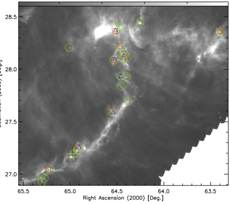
This procedure resulted in a total of 496 cores over the observed $2^{\circ}\!\!.2\times 2^{\circ}\!\!.2$ region. The total mass, 88 $M_{\odot}$, of the detected cores represents approximately 4% of the mass of the L1495 cloud, estimated to be 1500–2700 $M_{\odot}$ (Kramer & Winnewisser, 1991). From this set, 20 cores were selected for detailed study. The main goal of the final selection process was to obtain a list of relatively unconfused cores, uniformly sampled in mass according to preliminary estimates obtained via SED fitting as outlined in the next section. Cores which were multiply peaked or confused, based on visual examination of the 250–500 $\mu$m images, were excluded. The mass range 0.02–2.0 $M_{\odot}$ was then divided into seven bins, each of which spanned a factor of two in mass, and a small number of objects (nominally three) selected from each bin. The selection was made on a random basis except for a preference for objects for which previously-published data were available, thus facilitating comparison of deduced parameters. Fig. 1 shows the locations of the 20 selected cores on a SPIRE 250 $\mu$m image of the field.

Figure 1: SPIRE 250 $\mu$m image of the L1495 region. The green circles represent the locations of the 20 cores selected for modeling. The other symbols represent previously published core locations at other wavelengths; red squares: H¹³CO⁺ (Onishi et al., 2002); blue triangles: N₂H⁺ (Hacar et al., 2013); yellow cross: 850 $\mu$m (Sadavoy et al., 2010). The image is shown on a truncated intensity scale in order to emphasize faint structure; the display saturates at 200 MJy sr^-1 which corresponds to 100% on the greyscale.

4 SED fitting

Preliminary values of core masses and dust temperatures are estimated by fitting a greybody spectrum to the observed spectral energy distribution (SED) constructed from the set of five-wavelength getsources fluxes. For this computation, sources are assumed to be isothermal and have a wavelength variation of opacity of the form (Hildebrand, 1983; Roy et al., 2013):

$$\kappa(\lambda)=0.1\,(300/\lambda_{[\mu{\rm m}]})^{2}\qquad{\rm cm}^{2}\,{\rm g}^{-1}$$ (1)

Although obtained observationally, the numerical value of the coefficient in this relation is consistent with a gas to dust ratio of 100.

5 Core profiling

To obtain better estimates of core mass and other properties, a more detailed model fit is required. For this purpose we have developed a new procedure, COREFIT, which involves maximum likelihood estimation using both spatial and spectral information.

The fitting process involves calculating a series of forward models, i.e., sets of model images based on assumed parameter values, which are then compared with the data. The models are based on spherical geometry, in which the radial variations of volume density and temperature are represented by parametrized functional forms. For a given set of parameters, a model image is generated at each of the five wavelengths by calculating the emergent intensity distribution on the plane of the sky and convolving it with the instrumental point spread function (PSF) at the particular wavelength. The parameters are then adjusted to obtain an inverse-variance weighted least squares fit to the observed images.

In this procedure the wavelength variation of opacity is assumed to be given by Eq. (1) and the the radial variations of volume density and dust temperature are assumed to be described by Plummer-like (Plummer, 1911) and quadratic forms, respectively. Specifically we use:

$$n(r) = n_{0}/[1+(r/r_{0})^{\alpha}]$$ (2)

$$T(r) = T_{0}+(T_{1}\!-\!T_{0}\!-\!T_{2})r/r_{\rm out}+T_{2}(r/r_{\rm out})^{2}$$ (3)

where $n(r)$ represents the number density of H₂ molecules at radial distance $r$, $r_{0}$ represents the radius of an inner plateau, and $r_{\rm out}$ is the outer radius of the core, outside of which the core density is assumed to be zero. Also, $T_{0}$ is the central core temperature, $T_{1}$ is the temperature at the outer radius, and $T_{2}$ is a coefficient which determines the curvature of the radial temperature profile. In relating $n(r)$ to the corresponding profile of mass density we assume a mean molecular weight of 2.8 (Roy et al., 2013).

The set of unknowns then consists of: $n_{0}$, $r_{0}$, $r_{\rm out}$, $\alpha$, $T_{0}$, $T_{1}$, $T_{2}$, $x$, $y$, where the latter two variables represent the angular coordinates of the core centre. Representing this set by an 9-component parameter vector, p, we can write the measurement model as:

$${\bf\zeta}_{\lambda}={\bf f}_{\lambda}({\bf p})+b_{\lambda}+\nu_{\lambda}$$ (4)

where $\zeta_{\lambda}$ is a vector representing the set of pixels of the observed image at wavelength $\lambda$, ${\bf f}_{\lambda}({\bf p})$ represents the model core image for parameter set p, and $\nu_{\lambda}$ is the measurement noise vector, assumed to be an uncorrelated zero-mean Gaussian random process. Also, $b_{\lambda}$ represents the local background level, estimated using the histogram of pixel values in an annulus surrounding the source. This measurement model assumes implicitly that the core is optically thin at all wavelengths of observation.

In principle, the solution procedure is then to minimise the chi squared function, $\phi({\mathbf{p}})$, given by:

$$\phi({\mathbf{p}})=\sum_{\lambda,i}[(\zeta_{\lambda})_{i}-b_{\lambda}-({\bf f}_{\lambda}({\bf p}))_{i}]^{2}/\sigma_{\lambda}^{2}$$ (5)

where subscript $i$ refers to the $i$th pixel of the image at the given wavelength and $\sigma_{\lambda}$ represents the standard deviation of the measurement errors, evaluated from the sky background fluctuations in the background annulus.

In practice, two difficulties arise:

1. An unconstrained minimisation of $\phi({\mathbf{p}})$ is numerically unstable due to the fact that for a given total number of molecules, $n_{0}$ in Eq. (2) becomes infinite as $r_{0}\rightarrow 0$. It results in near-degeneracy such that the data do not serve to distinguish between a large range of possible values of the central density. To overcome this, we have modified the procedure to incorporate the constraint $r_{0}\geq r_{\rm min}$, where $r_{\rm min}$ is equal to one quarter of the nominal angular resolution, which we take to be the beamwidth at 250 $\mu$m. The estimate of central density then becomes a “beam-averaged” value over a resolution element of area $\pi r_{\rm min}^{2}$. For a distance of 140 pc, $r_{\rm min}$ corresponds to about 600 AU.

2. Most cores show some degree of asymmetry. This can degrade the quality of the global fit to a spherically-symmetric model, causing the centre of symmetry to miss the physical centre of the core. Some negative consequences include an underestimate of the central density and an overestimate of the central temperature. To alleviate this, we estimate the $(x,y)$ location of the core centre ahead of time using the peak of a column density map, constructed at the spatial resolution of the 250 $\mu$m image. The maximum likelihood estimation is then carried out using a 7-component parameter vector which no longer involves the positional variables.

Having performed the position estimation and constrained chi squared minimisation, the core mass is then obtained by integrating the density profile given by Eq. (2), evaluated using the estimated values of $n_{0}$, $r_{0}$ and $\alpha$.

Evaluation of the uncertainties in parameter estimates is complicated by the nonlinear nature of the problem which leads to a multiple-valley nature of $\phi({\mathbf{p}})$. The usual procedure, in which the uncertainty is evaluated by inverting a matrix of 2nd derivatives of $\phi({\mathbf{p}})$ (Whalen, 1971), then only provides values which correspond to the width of the global maximum and ignores the existence of neighbouring peaks which may represent significant probabilities. We therefore evaluate the uncertainties using a Monte Carlo technique in which we repeat the estimation procedure after adding a series of samples of random noise to the observational data and examine the effect on the estimated parameters.

We have also implemented an alternate version of COREFIT, referred to as “COREFIT-PH,” in which the dust temperature profile is based on a radiative transfer model, PHAETHON (Stamatellos & Whitworth, 2003), rather than estimating it from the observations. In this model, the radial density profile has the same form as for the standard COREFIT (Eq. (2)) but with the index, $\alpha$, fixed at 2. The temperature profile is assumed to be determined entirely by the heating of dust by the external ISRF; the latter is modeled locally as a scaled version of the standard ISRF (Stamatellos, Whitworth & Ward-Thompson, 2007) using a scaling factor, $\chi_{\rm ISRF}$, which represents an additional variable in the maximum likelihood solution.

We now compare the results obtained using the two approaches, both for synthetic and real data.

5.1 Tests with synthetic data

We have tested both COREFIT and COREFIT-PH against synthetic data generated using an alternate forward model for dust radiative transfer, namely MODUST (Bouwman et al., in preparation). Using the latter code, images at the five wavelengths were generated for a set of model cores and convolved with Gaussian simulated PSFs with full width at half maxima (FWHM) corresponding to the Herschel beamsizes. The models involved central number densities of $10^{5}$ cm^-3, $10^{6}$ cm^-3, and $3\times 10^{6}$ cm^-3 with corresponding $r_{0}$ values of 2500 AU, 4000 AU, and 1000 AU, respectively, and $r_{\rm out}$ values of $1.3\times 10^{4}$ AU, $1.7\times 10^{4}$ AU, and $1.2\times 10^{4}$ AU, respectively. The corresponding core masses were 0.59 $M_{\odot}$, 18.37 $M_{\odot}$, and 3.11 $M_{\odot}$, respectively. The synthesized images and corresponding Gaussian PSFs were then used as input data to the inversion algorithms. The results are presented in Table 1.

It is apparent that COREFIT gave masses and central temperatures in good agreement with the true model. While COREFIT-PH reproduced the central temperatures equally well, it underestimated the masses of these simulated cores by factors of 0.7, 0.5, and 0.5, respectively. The reason for these differences is that even though the two radiative transfer codes (PHAETHON and MODUST) yield central temperatures in good agreement with each other for a given set of model parameters, they produce divergent results for the dust temperatures in the outer parts of the cores, due largely to differences in dust model opacities. Since the outer parts comprise a greater fraction of the mass than does the central plateau region, this can lead to substantially different mass estimates given the same data. This problem does not occur for COREFIT since the latter obtains the temperature largely from the spectral variation of the data rather than from a physical model involving additional assumptions. These calculations thus serve to illustrate the advantages of simultaneous estimation of the radial profiles of dust temperature and density.

5.2 Results obtained with observational data

Table 2 shows the complete set of COREFIT parameter estimates for each of the Taurus cores. Also included are the assumed values of the inner radius of the annulus used for background estimation, equal to the getsources footprint size. Table 3 shows a comparison of the mass and temperature estimates amongst the different techniques, which include COREFIT and COREFIT-PH as well as the SED fitting discussed in Section 3. To facilitate comparison between the COREFIT temperatures and the mean core temperatures estimated from the spatially integrated fluxes used in the SED fits, we include the spatially averaged COREFIT temperature, $\bar{T}$, defined as the density-weighted mean value of $T(r)$ for $r\leq r_{\rm out}$. The COREFIT-PH results include the values of the ISRF scaling factor, $\chi_{\rm ISRF}$, the median value of which is 0.33. The fact that this is noticeably less than unity can probably be attributed to the fact that these cores are all embedded in filaments and hence the local ISRF is attenuated by overlying filamentary material. As an example of the fitting results, Figs. 2 and 3 show the estimated density and temperature profiles for core No. 2 in Table 2, based on COREFIT and COREFIT-PH, respectively.

Fig. 4 shows that the two techniques yield consistent estimates of masses, but the radiative transfer calculations produce central temperatures which are, on average, $\sim 2$ K lower than the COREFIT estimates. Although the difference is not significant in individual cases (the standard deviation being 1.4), it is clear from Fig. 4 that a systematic offset is present; the mean temperature difference, $\Delta T$, is $1.9\pm 0.3$ K.

Based on the results of testing with synthetic data, this difference seems too large to be explained by systematic errors associated with dust grain models, although we cannot rule out that possibility. One could also question whether our $\chi_{\rm ISRF}$ values are spuriously low. We do, in fact, find that by forcing the latter parameter to a somewhat larger value (0.5), the median $\Delta T$ can be reduced to zero with only a modest increase in the reduced chi squared, $\chi_{\nu}^{2}$ (0.85 as opposed to 0.83 for the best fit). The observations are completely inconsistent with $\chi_{\rm ISRF}=1.0$, however. As an additional test, we can take the COREFIT estimate of the radial density distribution for each core and use the standalone PHAETHON code to predict the central temperature for any assumed value of $\chi_{\rm ISRF}$. We thereby obtain consistency with the COREFIT estimates with $\chi_{\rm ISRF}=0.67$. However, this consistency comes at significant cost in terms of goodness of fit (the median $\chi_{\nu}^{2}$ increases to 2.27), and therefore does not serve to reconcile the COREFIT results with the expectations of radiative transfer. In summary, the COREFIT results are not entirely consistent with our assumed model for dust heating by the ISRF, but further work will be necessary to determine whether the differences are model-related or have astrophysical implications. So at this stage we have no evidence to contradict the findings of Evans et al. (2001) who considered various heating sources (the primary and secondary effects of cosmic rays and heating of dust grains by collisions with warmer gas particles) and concluded that heating by the ISRF dominates over all other effects.

How do the COREFIT estimates of temperature and mass compare with the preliminary values estimated from the getsources SEDs? In the case of temperature, the relevant comparison is between the SED-derived value and the spatially averaged COREFIT value; the data in Table 3 then give a mean “COREFIT minus SED” difference of -0.2 K, with a standard deviation of 1.1 for individual cores. The temperature estimates are thus consistent. With regard to mass, Fig. 5 shows that SED fitting under the isothermal assumption yields masses that are systematically smaller than the COREFIT values; the mean ratio of COREFIT mass to SED-based mass is 1.5, with a standard deviation of 1.0 in individual cases. Since the internal temperature gradient increases with the core mass, one might expect that the correction factor for SED-derived masses would increase with mass, although Fig. 5 has too much scatter to establish this. It may be evident when the results are averaged for a much larger statistical sample of cores, although the correction may well depend on environmental factors such as the intensity of the local ISRF.

Fig. 6 shows a plot of estimated central temperature as a function of core mass. Linear regression indicates that these quantities are negatively correlated with a coefficient of -0.64. This correlation can be explained quite naturally as a consequence of increased shielding of the core, from the ISRF, with increasing core mass. This being the case, one would expect an even stronger correlation with peak column density and this is confirmed by Fig. 7, for which the associated correlation coefficient is -0.86.

Fig. 8 shows a plot of $\alpha$ versus mass, where $\alpha$ is the index of radial density variation as defined by Eq. (2), and the masses are the COREFIT values. Given the relatively large uncertainties, the $\alpha$ values are, for the most part, consistent with values expected for Bonnor-Ebert spheres, whereby $\alpha=2.5$ provides an accurate empirical representation at radial distances up to the instability radius (Tafalla et al., 2004), and that $\alpha$ decreases to its asymptotic value of 2 beyond that.

Figure 2: Example of COREFIT results, for a 0.7 $M_{\odot}$ core in L1495 (No. 2 in Table 2). The solid lines indicate maximum likelihood estimates of the profiles of relative volume density and dust temperature. The dashed lines provide a measure of the uncertainty in the estimated density and temperature. They represent the results of a Monte Carlo simulation in which the estimation procedure is repeated 10 times after adding synthetic measurement noise to the observed images; the standard deviation of the added noise corresponds to the estimated measurement noise of the observed images.

Figure 3: COREFIT-PH results for the same core as in Fig. 2. In this variant of the estimation procedure, the dust temperature profile is modeled using a radiative transfer code (PHAETHON) instead of estimating it from the observations.

Figure 4: Comparison between parameter estimates, obtained using COREFIT and COREFIT-PH, for the 20 selected cores. In the former procedure, the dust temperature profile is estimated directly from the observations, while in the latter it is modeled using radiative transfer. Upper plot: COREFIT mass versus COREFIT-PH mass. For reference, the solid line represents the locus of equal masses. Lower plot: $\Delta T$ versus mass, where $\Delta T$ represents the difference in estimated temperature (COREFIT minus COREFIT-PH).

Figure 5: SED-derived mass based on isothermal assumption versus the mass from COREFIT model. For reference, the solid line represents the locus of equal masses.

Figure 6: Central dust temperature, $T_{0}$, as a function of core mass.

Figure 7: Central dust temperature, $T_{0}$, as a function of peak column density of H₂ molecules.

Figure 8: The estimated index of radial density falloff, $\alpha$, as a function of core mass.

The general consistency with the Bonnor-Ebert model is supported by the fact that when the maximum likelihood fitting procedure is repeated using the constraint $\alpha=2$, the chi squared values are, in most cases, not significantly different from the values obtained when $\alpha$ is allowed to vary. Two exceptions, however, are cores 2 and 13, both of which are fit significantly better by density profiles steeper than Bonnor-Ebert ($\alpha=3.1$ and 2.8, respectively), as illustrated by Fig. 9 for the former case. Specifically, the chi squared differences (17.2 and 7.5, respectively) translate into relative probabilities, for the “$\alpha\!=\!2$” hypothesis, of $\sim 2\times 10^{-4}$ and 0.02, respectively. If confirmed, such behaviour may have some important implications for core collapse models; a steepening of the density distribution in the early collapse phase is, in fact, predicted by the model of Vorobyov & Basu (2005) in which the collapsing core begins to detach from its outer boundary.

Figure 9: Radial profiles of the images of core No. 2 at four wavelengths, showing the match between observations and models for two different values of the radial density index, $\alpha$. Solid line: observed profile; dashed line: best fitting model ($\alpha=3.1$) convolved with the corresponding PSF at each wavelength); dotted line: same, except for the constraint $\alpha\!=\!2.0$. Note that the latter model results in a poor fit in the central region.

6 Core stability

Assessments of core stability are frequently made using SED-based estimates of core mass and temperature and observed source size, assuming that cores are isothermal and can be described as Bonnor-Ebert spheres (Lada et al., 2008). Using the SED-based data in Table 3 in conjunction with the getsources estimates of core size, we thereby find that the estimated core mass exceeds the Bonnor-Ebert critical mass for 10 of our 20 cores, suggesting that half of our cores are unstable to gravitational collapse.

Our COREFIT parameter estimates enable us to make a more detailed assessment of core stability based on a comparison with the results of hydrostatic model calculations that take account of the non-isothermal nature of the cores. This is facilitated by the modified Bonnor-Ebert (MBE) sphere models of Sipilä, Harju & Juvela (2011). Adopting their model curves, based on the Li & Draine (2001) grains which best reproduce our estimated core temperatures, the locus of critical non-isothermal models on a density versus mass plot is shown by the solid line on Fig. 10. Also plotted on this figure, for comparison, are the COREFIT estimates of those quantities. The seven points to the right of this curve represent cores that we would consider to be gravitationally unstable based on the modified Bonnor-Ebert models. Although this is somewhat less than the 10 that were classified as unstable based on the SED fits, the difference is probably not significant given that several points on the plot lie close to the “stability” line.

Figure 10: Central number density of H₂ molecules as a function of core mass. The circles represent the COREFIT estimates for L1495; filled symbols designate the subset of cores whose preliminary assessment of dynamical status suggests that they are gravitationally bound, based on getsources fluxes and sizes in conjunction with the standard model of isothermal Bonnor-Ebert spheres. For comparison, the solid line represents the locus of critically-stable non-isothermal Bonnor-Ebert spheres (Sipilä, Harju & Juvela (2011); points to the right of this line represent cores which are unstable to gravitational collapse according to that model.

The consistency between the above two procedures for stability assessment is illustrated by the fact that the MBE stability line in Fig. 10 provides a fairly clean demarcation between the cores classified as stable (open circles) and unstable (filled circles) from the simpler (SED-based) procedure. These results therefore suggest that prestellar cores can be identified reliably as such using relatively simple criteria.

The Bonnor-Ebert model also provides a stability criterion with respect to the centre-to-edge density contrast, whereby values greater than 14 indicate instability to gravitational collapse, both for the isothermal and non-isothermal cases (Sipilä, Harju & Juvela, 2011). However the outer boundaries are not well defined for the present sample of cores, and consequently the contrast values are uncertain in most cases. Two exceptions are cores 2 and 13, both of which have contrast estimates whose significance exceeds $3\sigma$. In both cases the mass exceeds the Bonnor-Ebert critical mass (by ratios of 1.2 and 6.0, respectively), and the centre-to-edge contrast values ($20\pm 6$ and $104\pm 32$, respectively) are in excess of 14. So for those two cores, at least, the core stability deduced from the density constrast is thus consistent with that assessed from total mass.

Table 1: Results of testing with synthetic data.

			$T_{0}$ [K]					Mass [$M_{\odot}$]					Peak H2 col. dens. [1022 cm-2]
Model			Std.	Alt.	True			Std.	Alt.	True			Std.	Alt.	True
1			10.1	8.6	10.0			0.61	0.39	0.59			0.59	0.45	1.04
2			6.8	6.5	6.5			22.7	9.48	18.4			23.9	5.65	16.1
3			7.8	6.5	6.7			3.30	1.46	3.11			7.95	4.91	13.4

Table 2: COREFIT parameter estimates for the 20 Taurus cores.

Core	RA	Dec	$r_{\rm annulus}$	$r_{0}$	$r_{\rm out}$	$n_{0}$	$\alpha$	$T_{0}$	$T_{1}$	$T_{2}$
No.	(J2000)	(J2000)	[$10^{3}$ AU]	[$10^{3}$ AU]	[$10^{3}$ AU]	[$10^{5}$ cm-3]		[K]	[K]	[K]
1	04:13:35.8	+28:21:11	7.56	$3.5\pm 1.2$	$7.1\pm 0.2$	$0.5\pm 0.1$	$2.0\pm 0.6$	$9.5\pm 0.5$	$11.2\pm 0.1$	$-1.4\pm 0.6$
2	04:17:00.6	+28:26:32	16.38	$4.7\pm 0.2$	$13.2\pm 0.6$	$0.7\pm 0.1$	$3.1\pm 0.4$	$10.7\pm 0.3$	$12.5\pm 0.2$	$-1.2\pm 0.2$
3	04:17:32.3	+27:41:27	11.20	$3.5\pm 3.1$	$7.3\pm 0.4$	$0.2\pm 0.1$	$2.0\pm 1.0$	$12.3\pm 0.8$	$13.1\pm 1.2$	$0.2\pm 0.1$
4	04:17:35.2	+28:06:36	10.30	$0.6\pm 0.2$	$8.4\pm 0.4$	$9.9\pm 2.9$	$3.7\pm 0.2$	$7.1\pm 0.6$	$23.7\pm 1.2$	$-2.6\pm 0.5$
5	04:17:36.2	+27:55:46	13.20	$2.9\pm 1.0$	$11.8\pm 0.4$	$0.8\pm 0.3$	$2.6\pm 0.4$	$9.4\pm 0.4$	$12.0\pm 0.3$	$-2.3\pm 0.5$
6	04:17:41.8	+28:08:47	10.08	$0.8\pm 0.2$	$8.8\pm 1.2$	$26\pm 18$	$2.0\pm 0.4$	$7.0\pm 0.1$	$8.3\pm 0.4$	$-1.1\pm 0.3$
7	04:17:43.2	+28:05:59	7.14	$1.0\pm 0.4$	$6.9\pm 0.2$	$13\pm 6$	$2.6\pm 0.3$	$7.1\pm 0.4$	$10.1\pm 0.2$	$-2.9\pm 0.5$
8	04:17:49.4	+27:50:13	8.10	$2.9\pm 2.9$	$7.7\pm 0.2$	$0.5\pm 0.2$	$1.9\pm 1.8$	$9.9\pm 1.6$	$10.8\pm 0.5$	$0.9\pm 0.6$
9	04:17:50.6	+27:56:01	13.86	$4.5\pm 0.2$	$10.4\pm 0.4$	$1.9\pm 0.1$	$3.4\pm 0.6$	$8.0\pm 0.2$	$10.1\pm 0.2$	$-1.0\pm 0.2$
10	04:17:52.0	+28:12:26	12.60	$4.3\pm 1.7$	$11.2\pm 0.2$	$0.9\pm 0.4$	$2.2\pm 0.6$	$10.0\pm 0.6$	$9.7\pm 0.6$	$-0.1\pm 0.3$
11	04:17:52.5	+28:23:43	12.15	$2.1\pm 1.0$	$9.5\pm 0.2$	$1.0\pm 0.3$	$1.9\pm 0.4$	$9.8\pm 0.6$	$11.2\pm 0.3$	$-0.4\pm 0.2$
12	04:18:03.8	+28:23:06	8.75	$2.3\pm 0.6$	$8.6\pm 0.2$	$2.3\pm 0.4$	$3.0\pm 0.9$	$9.9\pm 1.1$	$10.8\pm 1.1$	$0.9\pm 0.7$
13	04:18:08.4	+28:05:12	13.86	$2.3\pm 0.8$	$13.4\pm 0.2$	$6.8\pm 1.8$	$2.8\pm 0.4$	$6.0\pm 0.5$	$11.4\pm 0.3$	$-3.2\pm 0.5$
14	04:18:11.5	+27:35:15	7.45	$2.3\pm 1.4$	$7.3\pm 0.2$	$1.9\pm 0.5$	$2.0\pm 0.5$	$7.8\pm 0.4$	$10.1\pm 0.3$	$-2.2\pm 0.7$
15	04:19:37.6	+27:15:31	11.76	$2.7\pm 0.6$	$10.7\pm 0.4$	$1.6\pm 0.4$	$2.0\pm 0.2$	$8.8\pm 0.4$	$10.6\pm 0.1$	$-1.5\pm 0.2$
16	04:19:51.7	+27:11:33	9.24	$3.1\pm 0.4$	$8.9\pm 0.2$	$3.9\pm 0.5$	$3.4\pm 0.7$	$6.4\pm 0.2$	$9.6\pm 0.3$	$-3.0\pm 0.5$
17	04:20:02.9	+28:12:26	10.30	$1.4\pm 0.4$	$10.0\pm 0.4$	$0.5\pm 0.3$	$2.0\pm 0.3$	$10.7\pm 0.4$	$12.7\pm 0.2$	$-1.9\pm 0.5$
18	04:20:52.5	+27:02:20	5.30	$5.2\pm 2.9$	$5.2\pm 0.2$	$0.3\pm 0.1$	indet.	$11.4\pm 0.9$	$11.3\pm 0.4$	$0.1\pm 0.4$
19	04:21:06.8	+26:57:45	8.10	$2.7\pm 1.2$	$4.7\pm 0.6$	$0.6\pm 0.2$	$3.0\pm 1.2$	$11.1\pm 0.6$	$11.8\pm 0.2$	$0.1\pm 0.0$
20	04:21:12.0	+26:55:51	8.75	$2.9\pm 0.8$	$8.6\pm 0.2$	$0.3\pm 0.1$	$4.0\pm 1.2$	$10.1\pm 0.7$	$13.9\pm 0.1$	$-1.6\pm 0.6$

Table 3: Comparison of masses and temperatures estimated using the three different techniques discussed in the text

		SED-fitting				COREFIT					COREFIT-PH
Core		Mass	$T$			Mass	$T_{0}$	$\bar{T}$			Mass	$T_{0}$	$\chi_{\rm ISRF}$
No.		[$M_{\odot}$]	[K]			[$M_{\odot}$]	[K]	[K]			[$M_{\odot}$]	[K]
1		$1.19\pm 0.05$	$9.9\pm 0.3$			$0.20\pm 0.01$	$9.5\pm 0.5$	10.8			0.25	8.2	0.28
2		$0.71\pm 0.04$	$11.8\pm 0.5$			$0.84\pm 0.04$	$10.7\pm 0.3$	11.8			0.72	8.4	0.90
3		$0.10\pm 0.01$	$12.3\pm 0.5$			$0.09\pm 0.04$	$12.3\pm 0.8$	12.7			0.23	9.1	0.37
4		$0.05\pm 0.01$	$12.6\pm 0.8$			$0.04\pm 0.01$	$7.1\pm 0.6$	9.3			0.08	9.1	0.29
5		$0.20\pm 0.01$	$11.3\pm 0.1$			$0.37\pm 0.02$	$9.4\pm 0.4$	10.9			0.32	8.0	0.37
6		$1.01\pm 0.15$	$8.0\pm 0.6$			$1.70\pm 0.34$	$7.0\pm 0.1$	7.7			1.64	5.0	0.26
7		$0.22\pm 0.10$	$8.8\pm 1.1$			$0.49\pm 0.09$	$7.1\pm 0.4$	8.6			0.37	6.0	0.31
8		$0.07\pm 0.01$	$9.9\pm 1.5$			$0.19\pm 0.04$	$9.9\pm 1.6$	10.3			0.25	6.7	0.14
9		$1.53\pm 0.02$	$9.2\pm 0.1$			$1.44\pm 0.09$	$8.0\pm 0.2$	9.2			1.53	5.5	0.39
10		$1.30\pm 0.20$	$8.8\pm 0.9$			$0.96\pm 0.02$	$10.0\pm 0.6$	9.9			1.35	5.8	0.32
11		$0.20\pm 0.03$	$11.8\pm 1.1$			$0.32\pm 0.06$	$9.8\pm 0.6$	10.6			0.41	7.4	0.29
12		$0.42\pm 0.05$	$9.2\pm 0.6$			$0.41\pm 0.06$	$9.9\pm 1.1$	10.1			0.40	6.6	0.39
13		$1.60\pm 0.28$	$8.8\pm 1.0$			$2.03\pm 0.16$	$6.0\pm 0.5$	8.3			2.21	5.4	0.32
14		$0.47\pm 0.11$	$8.8\pm 1.7$			$0.46\pm 0.05$	$7.8\pm 0.4$	9.4			0.33	6.7	0.25
15		$0.21\pm 0.07$	$11.2\pm 1.9$			$0.84\pm 0.08$	$8.8\pm 0.4$	10.0			1.04	6.1	0.36
16		$0.36\pm 0.06$	$8.7\pm 0.5$			$1.08\pm 0.12$	$6.4\pm 0.2$	8.3			1.52	5.0	0.26
17		$0.05\pm 0.01$	$12.5\pm 1.2$			$0.08\pm 0.01$	$10.7\pm 0.4$	11.9			0.12	8.8	0.18
18		$0.21\pm 0.03$	$9.6\pm 0.8$			$0.09\pm 0.02$	$11.4\pm 0.9$	11.3			0.07	9.2	0.25
19		$0.08\pm 0.01$	$11.8\pm 0.8$			$0.08\pm 0.02$	$11.1\pm 0.6$	11.5			0.09	8.6	0.38
20		$0.02\pm 0.01$	$13.6\pm 0.7$			$0.06\pm 0.01$	$10.1\pm 0.7$	11.8			0.05	10.2	0.28

7 Comparison with previous observations

The deduced physical properties of our cores may be compared with previously published spectral line data in H¹³CO⁺ and N₂H⁺, both of which are known to be good tracers of high density gas ($n({\rm H}_{2})\stackrel{{\scriptstyle>}}{{{}_{\sim}}}10^{5}$ cm^-3). Of our 20 cores, we find accompanying observations for 10 in H¹³CO⁺ (Onishi et al., 2002) and seven in N₂H⁺ (Hacar et al., 2013). The relevant parameters are given in Table 4.

Table 4: Comparison with previously published spectral line data.

Core	ID			Offset [arcsec]			Radius [pc]				Mass [$M_{\odot}$]			$n$(H2) [$10^{5}$ cm-3]
No.	Onishi	Hacar		H13CO+	N2H+		Dust	H13CO+	N2H+		Dust	H13CO+		Dust	H13CO+
1	3	…		41	…		0.034	0.021	…		0.2	1.7		0.5	0.9
4	5	…		74	…		0.041	0.054	…		0.04	6.5		9.8	1.9
6	5	1		93	43		0.043	0.054	0.048		1.7	6.5		25	1.9
7	5	…		91	…		0.034	0.054	…		0.5	6.5		13	1.9
9	…	2		…	8.4		0.050	…	0.027		1.4	…		1.9	…
10	6	…		52	…		0.054	0.034	0.051		1.0	5.8		0.9	1.2
12	7	5		82	31		0.042	0.035	0.030		0.4	2.9		2.3	1.9
13	8	6		24	44		0.065	0.064	0.053		2.0	5.0		6.8	1.0
14	9	7		44	21		0.035	0.060	…		0.5	4.2		1.9	1.0
15	13a	10		8.0	19		0.052	0.048	0.047		0.8	3.4		1.6	1.4
16	…	12		…	9.4		0.043	…	0.034		1.1	…		3.9	…
18	16a	…		59	…		0.025	0.028	…		0.09	3.0		0.3	2.5

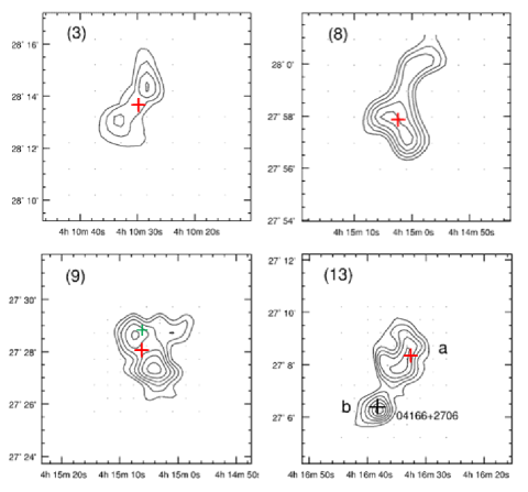
Considering first the H¹³CO⁺ data, comparison of observed peak locations with dust continuum source positions from COREFIT shows a distinct lack of detailed correspondence. This behaviour is apparent in Fig. 1 and from Table 4 which includes the angular distance (labeled as “Offset” in the table) between each of the H¹³CO⁺ source locations and the corresponding dust continuum core location. The median distance is $59^{\prime\prime}$, considerably larger than the spatial resolution of either the H¹³CO⁺ observations ($20^{\prime\prime}$) or the Herschel data ($18^{\prime\prime}$ at 250 $\mu$m). These offsets are somewhat surprising, since previous comparisons between H¹³CO⁺ and dust continuum maps have shown good correspondence (Umemoto et al., 2002). One could question whether they are due to gridding errors in the H¹³CO⁺ data, in view of the fact that the observations were made on a relatively coarse grid (the eight cores of Onishi et al. (2002) in Table 4 are split evenly between $30^{\prime\prime}$ and $60^{\prime\prime}$ grid spacings). However, the measured offsets show no correlation with the grid spacing—the mean offset is approximately $50^{\prime\prime}$ in either case; this argues against gridding error as an explanation. The most likely reason for the systematic offsets is that the H¹³CO⁺ is frozen out at the low ($\stackrel{{\scriptstyle<}}{{{}_{\sim}}}10$ K) temperatures of the core centres (Walmsley et al., 2004).

Detailed comparison of the dust continuum core locations with the H¹³CO⁺ maps (four examples of which are given in Fig. 10) shows that the majority of sources are elongated and/or double and that in some cases (Onishi core No. 3 in particular) the dust continuum source falls between the pair of H¹³CO⁺ components. In other cases (e.g. Onishi core No. 16a), the dust continuum peak falls on a nearby secondary maximum of the H¹³CO⁺ emission. In the latter case, surprisingly, the main peak of H¹³CO⁺ falls in a local minimum of dust emission. Comparisons between H¹³CO⁺ images and their 250 $\mu$m counterparts show that, in general, the elongation and source alignment in H¹³CO⁺ is along the filament, so we have a rod-like, rather than spherical, geometry. The picture which thus emerges is that when a core forms in a filament (André et al., 2010), we see the core centre in dust continuum emission and the warmer (but still dense, $\sim 10^{5}$ cm^-3) H¹³CO⁺ gas on either side of it in a dumbbell-like configuration. The median separation of the dust continuum and H¹³CO⁺ sources then corresponds to the typical radius of the depletion zone. For an ensemble of randomly oriented filaments, the mean projected separation is $\pi/4$ times the actual separation, which means that our estimated median separation of $59^{\prime\prime}$ corresponds to an actual separation of $75^{\prime\prime}$, or about $1.1\times 10^{4}$ AU at the distance of L1495. This is similar to the radius of the dark-cloud chemistry zone in which carbon-bearing molecules become gaseous (Caselli, 2011).

Figure 11: Examples of dust continuum core locations in relation to H¹³CO⁺ emission. The estimated locations of cores 1, 13, 14 and 15 (corresponding to Onishi core Nos. 3, 8, 9, and 13a, respectively) are superposed on H¹³CO⁺ maps taken from Onishi et al. (2002) (B1950 coordinates). In each case, the location of peak dust column density is indicated by a red cross. The green cross in Onishi field (9) represents a secondary peak of dust emission. The black cross in Onishi field (13) represents a protostar location.

Comparing the estimated masses, Table 4 shows that the values estimated from dust continuum observations are, in most cases, much smaller than those based on H¹³CO⁺. The discrepancy ranges from a factor of $\sim 2$ to more than an order of magnitude. Based on the mass and positional discrepancies it is clear that H¹³CO⁺ and submillimetre continuum are not mapping the same structures. Nevertheless, it remains to explain why so much of the expected dust emission from the H¹³CO⁺ emitting gas is apparently not being seen in the submillimetre continuum. It is unlikely to be a result of the background subtraction in COREFIT since the COREFIT mass estimates match the SED-based values from getsources fluxes within $\sim 30$% and the only background that was subtracted during the latter processing corresponded to the natural spatial scale of the broader underlying emission structure.

The most likely explanation for the discrepancy is an overestimation of the virial mass of the gas component due, in part, to the assumption by Onishi et al. (2002) of uniform velocity dispersion. Specifically, the velocity dispersion of the relatively cool gas being probed by dust emission is likely to be at least a factor of two lower than that of H¹³CO⁺, as suggested by the N₂H⁺ observations of Hacar et al. (2013), and since the estimated virial mass depends on the square of that dispersion, it could have been overestimated by a factor of up to 4. Two additional effects, both of which are likely to have led to overestimation of the virial mass are:

1. the Onishi et al. (2002) virial mass was based on assumed spherical shape as opposed to the filamentary geometry observed, and hence the source volumes may have been overestimated;

2. Onishi et al. (2002) assumed a constant density value for each core. However, virial models involving this assumption are likely to lead to overestimates of mass in cases where the actual density decreases outwards (MacLaren, Richardson & Wolfendale, 1988).

While the H¹³CO⁺ peaks do not correlate well with the dust continuum, the situation is different for N₂H⁺. This behaviour can be seen from Table 4 which includes the positional offsets between N₂H⁺ and dust continuum peaks; the median offset is only $21^{\prime\prime}$, i.e., only a third of the corresponding value for H¹³CO⁺ even though the resolution of the N₂H⁺ observations ($60^{\prime\prime}$) was much coarser. Thus the positional data provide no evidence for N₂H⁺ freeze-out, and this is supported by the fact that the N₂H⁺ detections seem preferentially associated with the coldest cores (the seven N₂H⁺ detections include four of our five lowest-temperature cores, all of which are cooler than 7 K). However, at higher resolution the situation may be different, since interferometric observations of $\rho$ Oph have shown that the correspondence between dust emission and N₂H⁺ clumps does indeed break down on spatial scales $\stackrel{{\scriptstyle<}}{{{}_{\sim}}}10^{\prime\prime}$ (Friesen et al., 2010). Theoretical models have, in fact, shown that within $\sim 1000$ AU of the core centre, complete freeze-out of heavy elements is likely (Caselli, 2011). Core profiling based on dust emission thus promises to make an important contribution to investigations of core chemistry by providing an independent method for estimating temperatures in the centres of cores.

Finally, our core No. 16 has been observed previously in the 850 $\mu$m continuum by Sadavoy et al. (2010) and given the designation JCMTSF_041950.8+271130. While the quoted 850 $\mu$m source radius of 0.019 pc is close to the COREFIT $r_{0}$ value of $0.015\pm 0.002$ pc, the estimated masses are significantly different. The estimate of Sadavoy et al. (2010) is based on the observed 850 $\mu$m flux density and an assumed dust temperature of 13 K; this yielded 0.22 $M_{\odot}$ which is a factor $\sim 5$ smaller than our COREFIT value and most likely an underestimate resulting from too high an assumed temperature. This illustrates the large errors in mass which can occur in the absence of temperature information, as has been noted by others (Stamatellos, Whitworth & Ward-Thompson, 2007; Hill et al., 2009, 2010).

8 Conclusions

The principal conclusions from this study can be summarised as follows:

1. For this sample of cores, the dust temperatures estimated from SED fits, using spatially integrated fluxes and an isothermal model, are consistent with the spatially averaged temperatures derived from the COREFIT profiles. However, the masses obtained from the SED fits are systematically lower (by a factor of $\sim 1.5$) than those obtained from detailed core profiling. The present statistical sample, however, is insufficient to obtain a definitive correction factor, the latter of which is likely to be dependent on mass and possibly environment (ISRF) also.

2. Estimates of central dust temperature are in the range 6–12 K. These temperatures are negatively correlated with peak column density, consistent with behaviour expected due to shielding of core centre from the ISRF, assuming that the latter provides the sole heating mechanism. The model core temperatures obtained from radiative transfer calculations are, however, systematically $\sim 2$ K lower than the COREFIT estimates; it is not yet clear whether that difference has an astrophysical origin or is due to errors in model assumptions.

3. The radial falloff in density is, in the majority of cases, consistent with the $\alpha\simeq 2$ variation expected for Bonnor-Ebert spheres although exceptions are found in two cases, both of which appear to have steeper density profiles. Since both involve cores which are gravitationally unstable based on Bonnor-Ebert criteria, such behaviour may have implications for models of the early collapse phase.

4. The reliability of core stability estimates derived from isothermal models is not seriously impacted by the temperature gradients known to be present in cores. Thus the preliminary classification of cores as gravitationally bound or unbound can be based on relatively simple criteria, facilitating statistical studies of large samples.

5. Core locations do not correspond well with previously published locations of H¹³CO⁺ peaks, presumably because carbon-bearing molecules are frozen out in the central regions of the cores, most of which have dust temperatures below 10 K. The results suggest that the H¹³CO⁺ emission arises from dense gas in the filamentary region on either side of the core itself, in a dumbbell-like geometry, and that the radius of the sublimation zone is typically $\sim 10^{4}$ AU.

6. The coldest cores are mostly detected in N₂H⁺, and the N₂H⁺ core locations are consistent with those inferred from dust emission, albeit at the relatively coarse ($1^{\prime}$) resolution of the N₂H⁺ data. Our data therefore do not show evidence of N₂H⁺ freeze-out.

References

- André, Ward-Thompson & Motte (1996) André, P., Ward-Thompson, D., Motte, F. 1996, A&A, 314, 625
- André et al. (2010) André, P., Men’shchikov, A., Bontemps, S., et al. 2010, A&A, 518, L102
- Caselli (2011) Caselli, P. 2011, in José Cernicharo & Rafael Bachiller, eds., Proc. IAU Symposium No. 280, 19
- Elias (1978) Elias, J. H. 1978, ApJ, 224, 857
- Evans et al. (2001) Evans, N. J. II, Rawlings, J. M. C., Shirley, Y. L. & Mundy, L. G. 2001, ApJ, 557, 193
- Friesen et al. (2010) Friesen, R. K., Di Francesco, J., Shimajiri, Y. & Takakuwa, S. 2010, ApJ, 708, 1002
- Giannini et al. (2012) Giannini, T., Elia, D., Lorenzetti, D. et al. 2012, A&A, 539, A156
- Griffin et al. (2010) Griffin, M. J., Abergel, A., Abreu, A., et al. 2010, A&A, 518, L3
- Griffin et al. (2013) Griffin, M. J., North, C. E., Amaral-Rogers, A. et al. 2013, MNRAS, 434, 992
- Hacar et al. (2013) Hacar, A., Tafalla, M., Kauffmann, J. & Kovács, A. 2013, A&A, 554, 55
- Hildebrand (1983) Hildebrand, R. H. 1983, QJRAS, 24, 267
- Hill et al. (2009) Hill, T., Pinte C., Minier, V., Burton, M. G., Cunningham, M. R. 2009 MNRAS, 392, 768
- Hill et al. (2010) Hill, T., Longmore, S. N., Pinte, C., Cunningham, M. R., Burton, M. G., Minier, V. 2010, MNRAS, 402, 2682
- Kirk et al. (2013) Kirk, J. M., Ward-Thompson, D., Palmeirim, P. et al. 2013, MNRAS, 432, 1424
- Könyves et al. (2010) Könyves, V., André, P., Men’shchikov, A., et al. 2010, A&A, 518, L106
- Kramer & Winnewisser (1991) Kramer, C. & Winnewisser, G. 1991, A&AS, 89, 42
- Lada et al. (2008) Lada, C. J., Muench, A. A., Rathborne, J., Alves, J. F., & Lombardi, M. 2008, ApJ, 672, 410
- Li & Draine (2001) Li, A., Draine, B. T. 2001, ApJ, 554, 778
- Lutz (2012) Lutz, D. 2012, Herschel Document PICC-ME-TN-033
- MacLaren, Richardson & Wolfendale (1988) MacLaren, I., Richardson, K. M., Wolfendale, A. W. 1988, ApJ, 333, 821
- Men’shchikov et al. (2012) Men’shchikov, A., André, Ph., Didelon, P. et al. 2012, A&A, 542, 81
- Motte, André & Neri (1998) Motte, F., André, Neri, R. 1998, A&A 336, 150
- Motte et al. (2010) Motte, F., Zavagno, A., Bontemps, S., et al. 2010, A&A 518, L77
- Onishi et al. (2002) Onishi, T., Mizuno, A, Kawamura, A et al. 2002, ApJ 575, 950
- Ott (2010) Ott, S., 2010, in Y. Mizumoto, K.-I. Morita, & M. Ohishi ed., Astronomical Data Analysis Software and Systems XIX Vol. 434 of ASP Conference Series, The Herschel Data Processing System – HIPE and Pipelines – Up and Running Since the Start of the Mission, p. 139 Mizuno, A, Kawamura, A et al. 2002, ApJ 575, 950
- Palmeirim et al. (2013) Palmeirim, P., André, Ph., Kirk, J. et al. 2013, A&A, 550, A38
- Pilbratt et al. (2010) Pilbratt, G. L., Riedinger, J. R., Passvogel, T., et al. 2010, A&A 518, L1
- Plummer (1911) Plummer, H. C. 1911, MNRAS, 71, 460
- Poglitsch et al. (2010) Poglitsch, A., Waelkens, C., Geis, N., et al. 2010, A&A, 518, L2
- Roussel (2013) Rousel, H. 2013, arXiv:1205.2576; PASP (in press)
- Roy et al. (2013) Roy, A., André, Ph., Palmeirim, P., et al. 2013, A&A, submitted
- Sadavoy et al. (2010) Sadavoy, S. I., Di Francesco, J., Bontemps, S., et al. 2010, ApJ, 710, 1247
- Sipilä, Harju & Juvela (2011) Sipilä, O., Harju, J., Juvela, M. 2011, A&A, 535, 49
- Stamatellos & Whitworth (2003) Stamatellos, D. & Whitworth, A. P. 2003, A&A, 407, 941
- Stamatellos, Whitworth & Ward-Thompson (2007) Stamatellos, D., Whitworth, A. P., Ward-Thompson, D. 2007, MNRAS, 379, 1390
- Tafalla et al. (2004) Tafalla, M., Myers, P. C., Caselli, P., & Walmsley, C. M. 2004, A&A, 416, 191
- Umemoto et al. (2002) Umemoto, T., Kamazaki, T., Sunada, K., Kitamura, Y. & Hasegawa, T. 2002, in Proc. IAU 8th Asian-Pacific Regional Meeting, ASJ, Vol. II, 229
- Vorobyov & Basu (2005) Vorobyov, E. I. & Basu, S., 2005, MNRAS, 360, 675
- Walmsley et al. (2004) Walmsley, C. M., Flower, D. R. & Pineau Des Forêts, G. 2004, in S. Pfalzner et al. (eds.) The Dense Interstellar Medium in Galaxies, Proc. 4th Cologne-Bonn-Zermatt Symposium, Springer Proceedings in Physics, 91, 467
- Ward-Thompson et al. (1994) Ward-Thompson, D., Scott, P. F., Hills, R. E., André, P., 1994, MNRAS, 268, 276
- Whalen (1971) Whalen, A. D. 1971, “Detection of Signals in Noise” (New York: Academic Press)