Dispersive Shock Waves in Viscously Deformable Media

Abstract

The viscously dominated, low Reynolds’ number dynamics of multi-phase, compacting media can lead to nonlinear, dissipationless/dispersive behavior when viewed appropriately. In these systems, nonlinear self-steepening competes with wave dispersion, giving rise to dispersive shock waves (DSWs). Example systems considered here include magma migration through the mantle as well as the buoyant ascent of a low density fluid through a viscously deformable conduit. These flows are modeled by a third-order, degenerate, dispersive, nonlinear wave equation for the porosity (magma volume fraction) or cross-sectional area, respectively. Whitham averaging theory for step initial conditions is used to compute analytical, closed form predictions for the DSW speeds and the leading edge amplitude in terms of the constitutive parameters and initial jump height. Novel physical behaviors are identified including backflow and DSW implosion for initial jumps sufficient to cause gradient catastrophe in the Whitham modulation equations. Theoretical predictions are shown to be in excellent agreement with long-time numerical simulations for the case of small to moderate amplitude DSWs. Verifiable criteria identifying the breakdown of this modulation theory in the large jump regime, applicable to a wide class of DSW problems, are presented.

1 Introduction

Shock waves in fluids typically arise as a balance between nonlinearity and dissipatively dominated processes, mediated by the second law of thermodynamics. An alternative balancing mechanism exists in approximately conservative media over time scales where dissipation is negligible. Nonlinearity and wave dispersion have been observed to lead to dynamically expanding, oscillatory dispersive shock waves (DSWs) in, for example, shallow water waves (known as undular bores) (Chanson, 2010), ion-acoustic plasma (known as collisionless shock waves) (Taylor et al., 1970; Tran et al., 1977), superfluids (Dutton et al., 2001; Hoefer et al., 2006), and “optical fluids” (Wan et al., 2007; Conti et al., 2009). It is therefore counterintuitive that a fluid driven by viscous forces could lead to shock waves regularized by dispersion. In this work, precisely this scenario is investigated in viscously deformable media realized in magma transport and viscous fluid conduits.

The description of a low viscosity fluid flowing through a viscously deformable, compacting medium is a fundamental problem in Earth processes. Such systems include flow of oil through compacting sediment, subterranean percolation of groundwater through a fluidized bed, or the transport of magma through the partially molten upper mantle (McKenzie, 1984). This type of flow also has implications for the buoyant ascent of a low density fluid through a deformable vertical conduit. Great interest by the broader scientific community has been taken in these systems since the derivation of a set of governing equations (McKenzie, 1984; Scott & Stevenson, 1984, 1986; Fowler, 1985). The primitive equations treat the magma transport as flow of a low Reynolds’ number, incompressible fluid through a more viscous, permeable matrix that is allowed to compact and distend, modeled as a compressible fluid. This model, thought to be a reasonable representation of melt transport in the upper mantle, contrasts with standard porous media flow where the matrix is assumed fixed and the fluid is compressible.

Upon reduction to one-dimension (1D) and under a number of reasonable simplifications, the model equations reduce to the dimensionless, scalar magma equation

$$\phi_{t}+(\phi^{n})_{z}-(\phi^{n}(\phi^{-m}\phi_{t})_{z})_{z}=0,$$ (1)

where $\phi$ is the porosity, or volume fraction of the solid matrix occupied by the magma or melt, and $(n,m)$ result from constitutive power laws relating the porosity to the matrix permeability and viscosity, respectively. Scott & Stevenson (1984, 1986) concluded that the parameter space for realistic magma systems is $n\in[2,5]$ and $m\in[0,1]$, a claim which was later supported by re-derivation of the conservation equations via homogenization theory for different geometric configurations of the flow (Simpson et al., 2010). The flow through a deformable vertical conduit, magma migration via thermal plumes through the convecting mantle being one example, can also be written in the form (1) upon taking $(n,m)=(2,1)$ with the interpretation of $\phi$ as the conduit’s cross-sectional area (Olson & Christensen, 1986).

The magma equation (1) is a conservation law for the porosity with nonlinear self-steepening due to buoyant advection through the surrounding matrix via the flux term $\phi^{n}$ and nonlocal dispersion due to compaction and distention of the matrix. Solitary traveling waves are special solutions to eq. (1) that have been studied in detail both theoretically (Scott & Stevenson, 1984, 1986; Richter & McKenzie, 1984; Barcilon & Richter, 1986; Nakayama & Mason, 1992; Simpson & Weinstein, 2008) and experimentally (Scott et al., 1986; Olson & Christensen, 1986; Helfrich & Whitehead, 1990). A natural generalization of single solitary waves to the case of a train of such structures can be realized as a DSW when the porosity exhibits a transition between two distinct states. The canonical dynamical problem of this type is the determination of the long time behavior of the dispersive Riemann problem, consisting of eq. (1) and the step initial data

$$\phi(z,0)=\begin{cases}\phi_{-},&z\in(-\infty,0]\\ \phi_{+},&z\in(0,\infty)\end{cases}.$$ (2)

Note that there is currently no rigorous proof of well-posedness for this particular initial value problem (Simpson et al., 2007).

The dispersive Riemann problem was first studied in numerical simulations of eq. (1) in the $(n,m)=(3,0)$ case by Spiegelman (1993a, b). Rather than smoothing the discontinuity and developing a classical shock front as in a dissipatively regularized system, the magma system responds to a jump by the generation of an expanding region of nonlinear oscillations with a solitary wave front and small amplitude tail, characteristic of DSWs (see figure 1). With the inclination to assume that steep gradients should be regularized by dissipative processes in this viscous system, Spiegelman (1993b) used classical shock theory (Whitham, 1974) to attempt to describe the behavior. In this work, we use a nonlinear wave averaging technique (El, 2005), referred to as Whitham averaging (Whitham, 1965), in order to describe the dispersive regularization of step initial data of arbitrary height with $0<\phi_{+}<\phi_{-}$ for a range of constitutive parameters $(n,m)$. The resulting DSW’s leading and trailing edge speeds are determined and the solitary wave front amplitude is resolved.

Traditional analysis of DSWs, first studied in the context of the Korteweg-de Vries (KdV) equation, asymptotically describes the expanding oscillatory region via the slow modulation of a rapidly oscillating, periodic traveling wave solution. These modulations are connected to the constant states of the exterior region by assuming the presence of linear dispersive waves at one edge of the DSW (amplitude $a\rightarrow 0$) and a solitary wave at the other (wavenumber $k\rightarrow 0$), as shown in figure 1 (Whitham, 1965; Gurevich & Pitaevskii, 1974). In the case of KdV, the resulting system of three hyperbolic modulation equations can be solved due to the availability of Riemann invariants, which are, in general, not available for non-integrable systems such as the one considered here. An extension of simple wave led DSW Whitham modulation theory to non-integrable systems has been developed by El (2005), which has been successfully applied, for example, to fully nonlinear, shallow water undular bores (El et al., 2006, 2009) and internal, two-fluid undular bores (Esler & Pearce, 2011). The modulation equations reduce exactly to a system of two hyperbolic equations at the leading and trailing edges where Riemann invariants are always available. Assuming the existence of an integral curve connecting trailing and leading edge states in the full system of modulation equations, one can calculate important physical DSW properties, namely the edge speeds, the solitary wave edge amplitude, and the trailing edge wavepacket wavenumber (see $s_{\pm}$, $a_{+}$, and $k_{-}$ in figure 1), with knowledge of only the reduced system at the leading and trailing edges. We implement this Whitham-El simple wave DSW theory for the magma dispersive Riemann problem, finding excellent agreement with full numerical simulations in the small to moderate jump regime. In the large jump regime, we identify novel DSW behavior including backflow (negative trailing edge speed, $s_{-}<0$) and DSW implosion. The oscillatory region of the implosion is characterized by slowly modulated periodic waves bookending an interior region of wave interactions. This behavior is associated with a change in sign of dispersion and gradient catastrophe in the Whitham modulation equations. To the best of our knowlege, this is the first example of breaking of the Whitham modulation equations for initial data of single step type, previous studies having focused on breaking for multistep initial data (Grava & Tian, 2002; Hoefer & Ablowitz, 2007; Ablowitz et al., 2009) or an initial jump in a modulated periodic wave’s parameters (Jorge et al., 1999), resulting in quasi-periodic or multi-phase behavior. Including gradient catastrophe, we identify four verifiable criteria that can lead to the breakdown of the simple wave DSW theory, applicable to DSW construction in other dispersive media.

Application of DSW theory to solutions of the magma equation has been largely neglected in the previous literature. Elperin et al. (1994) considered the weakly nonlinear KdV reduction of the magma equation and generic properties of the small amplitude DSWs produced. Marchant & Smyth (2005) numerically integrated the full Whitham modulation equations for the “piston” problem with $(n,m)=(3,0)$ incorporating a Dirichlet boundary condition rather than considering the general Riemann problem. Furthermore, key DSW physical parameters were not discussed in detail and neither backflow nor DSW implosion were observed. This work implements a general classification of weak to large amplitude DSW behavior in terms of the initial jump height and the constitutive parameters.

The presentation proceeds as follows. Section 2 describes the derivation of the magma equation from the full set of governing equations for both magma transport and viscous fluid conduits. Section 3 presents properties of the magma equation important to the application of Whitham theory. Section 4 implements Whitham theory to the problem at hand and its comparison with numerical simulations is undertaken in Section 5. Key physical consequences of solution structures are elucidated and influences of parameter variation are considered. Causes of breakdown in the analytical construction in the case of large jumps are identified. We conclude the manuscript with some discussion and future directions in Section 6.

Figure 1: Example numerical solution of the dispersive Riemann problem for eq. (1). The solution to the initial step connects the external constant states $\phi_{\pm}$ to an inner oscillatory region with a solitary wave leading edge where the wavenumber $k\rightarrow 0$ and a packet of linear waves in the trailing edge where $a\rightarrow 0$. The salient physical properties of a magma DSW are the leading edge amplitude $a_{+}$, trailing edge wavenumber $k_{-}$, the forward propagation speed of the solitary wave front $s_{+}$, and the trailing edge speed $s_{-}$.

2 Governing Equations

In this section, we briefly summarize the origin of the magma equation (1) in the context of magma migration (McKenzie, 1984; Scott & Stevenson, 1984, 1986) and fluid conduit flow (Olson & Christensen, 1986). Our purpose is to put the dispersive equation in its physical context in terms of assumptions, parameters, and scalings.

2.1 Magma Geophysics

The equations governing flow of a viscous interpenetrating fluid through a viscously deformable medium were derived independently in the context of magma by McKenzie (1984); Scott & Stevenson (1984, 1986); Fowler (1985). The system is a generalization of standard rigid body porous media flow but exhibits novel behavior. In the absence of phase transitions, buoyancy drives the predominant vertical advection of magma, the fluid melt, but the inclusion of dilation and compaction of the solid matrix introduces variability in the volume fraction occupied by the melt, which we will see transmits melt fluxes through the system as dispersive porosity waves. In the interest of providing physical intuition for understanding the 1D magma equation, we now recall the formulation of McKenzie and describe the derivation of conservation equations for mass and momentum of the fluid melt and the solid matrix, and then reduce systematically to eq. (1). In what follows, variable, primed quantities are unscaled, often dimensional. Unprimed variable quantities are all scaled and nondimensional. Material parameters and scales are unprimed as well.

The governing equations are a coupled set of conservation laws for mass and momentum which describe the melt as an inviscid, incompressible fluid and the solid matrix as a viscously deformable fluid, written in terms of the porosity $\phi^{\prime}$ (or volume fraction of melt). Interphase mass transfers are taken to be negligible so the coupling comes from McKenzie’s introduction of the interphase force $\mathbf{I}^{\prime}$, a generalization of the standard D’Arcy’s law (Scheidegger, 1974), which describes the rate of separation of the melt and matrix as proportional to the gradients of the lithostatic and fluid pressures. The leading proportionality term is chosen so that in the limit of a rigid matrix, D’Arcy’s Law is recovered. Upon substitution of the coupling term into the governing equations, the system reduces to the Stokes’ flow equations for the matrix in the “dry” limit, $\phi^{\prime}\rightarrow 0$.

To simplify clearly to the 1D magma equation, it is convenient to write the governing equations as in Katz et al. (2007), where the original McKenzie system is presented in a computationally amenable form. This follows from taking the solid and fluid densities to be distinct constants and then introducing a decomposition of the melt pressure $P^{\prime}=P_{\mathrm{l}}^{\prime}+\mathcal{P}^{\prime}+\left.P^{*}\right.^{\prime}$ where $P_{\mathrm{l}}^{\prime}=\rho_{\mathrm{s}}gz^{\prime}$ is the background lithostatic pressure, $\mathcal{P}^{\prime}$ is the pressure due to dilation and compaction of the matrix given by $\mathcal{P}^{\prime}=(\zeta^{\prime}-\frac{2}{3}\eta^{\prime})\nabla\cdot\boldsymbol{v}^{\prime}_{\mathrm{s}}$, and $\left.P^{*}\right.^{\prime}$ encompasses the remaining pressure contributions primarily stemming from viscous shear stresses in the matrix. Note the introduction of the solid matrix velocity $\boldsymbol{v}^{\prime}_{\mathrm{s}}$, as well as the matrix shear and bulk viscosities $\eta^{\prime},\zeta^{\prime}$, which arise due to matrix compressibility and depend on the porosity as described below. For nondimensionalization, we follow the scalings described in Spiegelman (1993a) (a similar reduction was performed in Scott & Stevenson (1984, 1986); Barcilon & Richter (1986); Barcilon & Lovera (1989)). This requires the introduction of the natural length scale of matrix compaction $\delta$ and the natural velocity scale of melt percolation $w_{0}$ proposed by McKenzie (1984), which for a background porosity $\phi_{0}$ are defined as

$$\delta=\sqrt{\frac{K^{\prime}_{0}(\zeta^{\prime}_{0}+\frac{4}{3}\eta^{\prime}_{0})}{\mu^{\prime}}},\quad w_{0}=K^{\prime}_{0}\frac{\Delta\rho g}{\phi_{0}\mu}$$ (3)

where $\mu$ is the melt viscosity, $\Delta\rho=\rho_{\mathrm{s}}-\rho_{\mathrm{f}}$ is the difference between the solid and fluid densities, and $K^{\prime}_{0}$ and $(\zeta^{\prime}_{0}+\frac{4}{3}\eta^{\prime}_{0})$ are the permeability and combined matrix viscosity at the background porosity $\phi_{0}$, respectively. Spiegelman et al. (2001) remarks that for practical geological problems, $\delta$ is on the order of $10^{2}-10^{4}$ m while $w_{0}$ takes on values of 1 - 100 $\mathrm{m~{}yr}^{-1}$, and the background porosity $\phi_{0}$ of standard media is between $10^{-3}-10^{-2}$. Using these as standard scales and after algebraic manipulation, the McKenzie system reduces to the non-dimensional form (unprimed variables) of the system presented in Katz et al. (2007),

$$\frac{D\phi}{Dt}=(1-\phi_{0}\phi)\frac{\mathcal{P}}{\xi},$$ (4)

$$-\nabla\cdot K\ \nabla\mathcal{P}+\frac{\mathcal{P}}{\xi}=\nabla\cdot K\ [\nabla P^{*}+\mathbf{\hat{g}}],$$ (5)

$$\nabla\cdot\boldsymbol{v}_{\mathrm{s}}=\phi_{0}\frac{\mathcal{P}}{\xi},$$ (6)

$$\nabla P^{*}=\nabla\cdot\eta(\nabla\boldsymbol{v}_{\mathrm{s}}+\nabla\boldsymbol{v}_{\mathrm{s}}^{\mathrm{T}})-\phi_{0}\phi\mathbf{\hat{g}},$$ (7)

where $\xi=\zeta-\frac{2}{3}\eta$ and $\mathbf{\hat{g}}$ is a unit vector in the direction of gravity. Neglecting terms $\textit{O}(\phi_{0})$, moving in the reference frame of the matrix, and introducing constitutive laws $K=\phi^{n}$ and $\xi=\phi^{-m}$ for the permeability and a combined matrix viscosity, the system (4)-(7) reduces to the dimensionless, 1D form for the vertical ascent of the fluid magma

$$\phi_{t}=\phi^{m}\mathcal{P},$$ (8)

$$-(\phi^{n}\mathcal{P}_{z})_{z}+\phi^{m}\mathcal{P}=-(\phi^{n})_{z}{\rm Phys.~{}Rev.~{}D}$$ (9)

After normalizing by the natural length and time scales (3), this system of equations conveniently has no coefficient dependence on adjustable parameters, which gives rise to a scaling symmetry discussed in Section 3.1. The constitutive power laws represent the expected effects of changes in the matrix porosity on its permeability and combined viscosity, when the porosity is small. Both physical arguments (c.f. Scott & Stevenson, 1984, 1986) and homogenization theory (Simpson et al., 2010) have been used to argue that physically relevant values for the constitutive parameters $(n,m)$ lie in the range $n\in[2,5]$ and $m\in[0,1]$ or at least in some subset of that range. Eliminating the compaction pressure from the above formulation, leads to the scalar magma equation (1) considered in this paper.

From the derivation, we observe that the time evolution of porosity in an interpenetrating magma flow system is controlled by a nonlinear advection term $(\phi^{n})_{z}$ and a dispersive term $(\phi^{n}(\phi^{-m}\phi_{t})_{z})_{z}$. The nonlinearity enters the system via buoyant forcing of the melt, driven by the matrix permeability. Compaction and dilation of the matrix generate dispersive effects on the melt which for step-like initial data, result in porosity propagation in the form of an expanding region of porosity waves.

2.2 Viscous Fluid Conduits

An independent formulation of eq. (1) arises in the context of a conduit of buoyant fluid ascending through a viscously deformable pipe. For magma, this represents an alternative transport regime to the interpenetrating flow described above, most closely related to flow up the neck of a thermal plume in the mantle.

Following Olson & Christensen (1986), the buoyant fluid rises along a vertical conduit of infinite length with circular cross-sections, embedded in a more viscous matrix fluid. The matrix with density $\rho_{\mathrm{M}}$, viscosity $\eta_{\mathrm{M}}$ and the fluid conduit with density $\rho_{\mathrm{f}}$, viscosity $\eta_{\mathrm{f}}$, must satisfy

$$\rho_{\mathrm{M}}>\rho_{\mathrm{f}}\quad\quad\eta_{\mathrm{M}}\gg\eta_{\mathrm{f}}{\rm Phys.~{}Rev.~{}D}$$ (10)

The circular cross-sectional area is $A^{\prime}=\pi R^{\prime 2}$, where the conduit radius $R^{\prime}$ is allowed to vary. The Reynolds’ number and slope of the conduit wall (i.e. the ratio of conduit deformation to wavelength) are assumed to be small and mass and heat diffusion are negligible.

With this set-up, the conduit flux $Q^{\prime}$ can be related to the cross-sectional area $A^{\prime}$ via Poiseuille’s Law for pipe flow of a Newtonian fluid (recall that primed variables are dimensional)

$$Q^{\prime}=-\frac{A^{\prime 2}}{8\pi\eta_{\mathrm{f}}}\frac{\partial P^{\prime}}{\partial z^{\prime}}$$ (11)

where $P$ is the nonhydrostatic pressure of the fluid. Conservation of mass manifests as

$$\frac{\partial A^{\prime}}{\partial t}+\frac{\partial Q^{\prime}}{\partial z}=0{\rm Phys.~{}Rev.~{}D}$$ (12)

To derive an expression for $P^{\prime}$, we balance radial forces at the conduit wall. Using the small-slope approximation, we assume radial pressure forces in the conduit dominate viscous effects. In the matrix, the radial components of the normal force dominate viscous stresses. Setting the radial forces of the matrix and conduit equal at the boundary and making the appropriate small-slope approximations, yields an expression for the nonhydrostatic pressure

$$P^{\prime}=-\Delta\rho gz^{\prime}+\frac{\eta_{\mathrm{M}}}{A^{\prime}}\frac{\partial A^{\prime}}{\partial t^{\prime}},$$ (13)

for $\Delta\rho=\rho_{\mathrm{M}}-\rho_{\mathrm{f}}$. Substitution of (13) back into (11), utilizing (12) for simplification and nondimensionalizing about a background, steady state, vertically uniform Poiseuille flow

$$Q_{0}=\frac{\Delta\rho g}{8\pi\eta_{\mathrm{f}}}A_{0}^{2},$$

with length and time scales $L$ and $T$

$$L=\left(\frac{\eta_{\mathrm{M}}A_{0}}{8\pi\eta_{\mathrm{f}}}\right)^{\frac{1}{2}},\quad T=\frac{1}{\Delta\rho g}\left(\frac{8\pi\eta_{\mathrm{f}}\eta_{\mathrm{M}}}{A_{0}}\right)^{\frac{1}{2}},$$

gives the non-dimensional equations

$$Q=A^{2}\left[1+\frac{\partial}{\partial z}\left(\frac{1}{A}\frac{\partial Q}{\partial z}\right)\right],$$

$$-\frac{\partial A}{\partial t}=\frac{\partial Q}{\partial z}{\rm Phys.~{}Rev.~{}D}$$

which are eqs. (8) and (9) for the case $(n,m)=(2,1)$.

3 Properties of the Magma Equation

In this section we recall several results that will be important for our studies of magma DSWs. It is interesting to note that for the pairs $(n,m)=(-1,0)$ and $(n,m)=(\frac{1}{2},\frac{1}{2})$ the magma equation has been shown to be completely integrable, but for other rational values of $(n,m)$ it is believed to be non-integrable by the Painleve ODE test (Harris & Clarkson, 2006). We will primarily be concerned with the physically relevant non-integrable range $m\in[0,1],n\in[2,5]$, but many of the results are generalized to a much wider range of values.

3.1 Linear Dispersion Relation and Scaling

Linearizing eq. (1) about a uniform background porosity $\Phi$ and seeking a harmonic solution with real-valued wavenumber $k$, and frequency $\omega_{0}$, we write $\phi$ as

$$\phi(z,t)\approx\Phi+\nu\left(e^{i(kz-\omega_{0}t)}+\mathrm{c.c.}\right),\quad\left|\nu\right|\ll 1,$$ (14)

where $\mathrm{c.c.}$ denotes the complex conjugate. Substitution into eq. (1) yields the linear dispersion relation

$$\omega_{0}(k,\Phi)=\frac{n\Phi^{n-1}k}{1+\Phi^{n-m}k^{2}}{\rm Phys.~{}Rev.~{}D}$$ (15)

Taking a partial derivative in $k$ gives the group velocity

$$(\omega_{0}(k,\Phi))_{k}=\frac{n\Phi^{n-1}(1-\Phi^{n-m}k^{2})}{(1+\Phi^{n-m}k^{2})^{2}}{\rm Phys.~{}Rev.~{}D}$$ (16)

Note that although the phase velocity $\frac{\omega_{0}}{k}$ is strictly positive, the group velocity (16) can take on either sign, with a change in sign occurring when $k^{2}=\Phi^{m-n}$. Taking a second partial derivative of eq. (15) with respect to $k$ gives

$$(\omega_{0}(k,\Phi))_{kk}=\frac{-2nk\Phi^{2n-1-m}(3-\Phi^{n-m}k^{2})}{(1+\Phi^{n-m}k^{2})^{3}}{\rm Phys.~{}Rev.~{}D}$$ (17)

Introducing the sign of dispersion, we say the system has positive dispersion if $(\omega_{0}(k,\Phi))_{kk}>0$ so that the group velocity is larger for shorter waves. Similarly, negative dispersion is defined as $(\omega_{0}(k,\Phi))_{kk}<0$. From eq. (17), the sign of dispersion is negative for long waves but switches to to positive when $k^{2}=3\Phi^{m-n}$. These distinguished wavenumbers, the zeros of the group velocity and sign of dispersion, have physical ramifications on magma DSWs that will be elucidated later.

The magma equation also possesses a scaling symmetry. It is invariant under the change of variables

$$\phi^{\prime}=\Phi\phi,\quad z^{\prime}=\Phi^{\frac{n-m}{2}}z,\quad t^{\prime}=\Phi^{\frac{1}{2}(2-n-m)}t,\quad\Phi>0{\rm Phys.~{}Rev.~{}D}$$ (18)

This allows us to normalize the background porosity to one without loss of generality, which we will do in Section 4.

3.2 Long Wavelength Regime

In the weakly nonlinear, long wavelength regime, the magma equation reduces to the integrable KdV equation (Whitehead & Helfrich, 1986; Takahashi et al., 1990; Elperin et al., 1994) . To obtain KdV we enter a moving coordinate system with the linear wave speed $n$ and introduce the “slow” scaled variables $\zeta=\varepsilon^{1/2}(z-nt)$, $\tau=\varepsilon^{3/2}t$, and $\phi(z,t)=1+\varepsilon u(z,t)$ to the magma equation. Assuming $|\varepsilon|\ll 1$, a standard asymptotic calculation results in

$$u_{\tau}+n(n-1)uu_{\zeta}+nu_{\zeta\zeta\zeta}=0,$$ (19)

which has no dependence on the parameter $m$. What this implies physically is that dispersion in the small amplitude, weakly nonlinear regime is dominated by matrix compaction and dilation. Nonlinear dispersive effects resulting from matrix viscosity are negligible. The original construction of a DSW was undertaken for KdV by Gurevich & Pitaevskii (1974). In Section 4, we will compare the results of KdV DSW theory with our results for magma DSWs.

3.3 Nonlinear Periodic Traveling Wave Solutions

The well-studied solitary waves of eq. (1) are a limiting case of more general periodic traveling wave solutions. To apply Whitham theory to the magma equation, it is necessary to derive the periodic traveling wave solution to eq. (1), which forms the basis for nonlinear wave modulation. In the special case $(n,m)=(3,0)$, Marchant & Smyth (2005) obtained an implicit relation for $\phi$ in terms of elliptic functions, and for $(n,m)=(2,1)$, the equation was derived in integral form by Olson & Christensen (1986). Here we consider the full physical range of the constitutive parameters.

We seek a solution of the form $\phi(z,t)=\phi(\theta)$, where $\theta=z-ct$ for wave velocity $c$ ($c$ is related to the wave frequency $\omega$ and the wavenumber $k$ by the relation $\omega=ck$), such that $\phi(\theta)=\phi(\theta+L)$ with wavelength $L$. Inserting this ansatz into eq. (1) and integrating once yields

$$c(\phi^{-m}\phi^{\prime})^{\prime}=A\phi^{-n}+c\phi^{1-n}-1,$$ (20)

for integration constant $A$ and ^′ indicating a derivative with respect to $\theta$. Observing

$$c(\phi^{-m}\phi^{\prime})^{\prime}=c\left(\frac{1}{2}\phi^{m}\right)\left[\frac{d}{d\phi}\left(\phi^{-2m}(\phi^{\prime})^{2}\right)\right],$$

enables us to integrate with respect to $\phi$ and find for $m\neq 1$ and $n+m\neq 2$

$$(\phi^{\prime})^{2}=\frac{2}{2-m-n}\phi^{m-n+2}-\frac{2}{c(1-m)}\phi^{m+1}-\frac{2A}{c(1-m-n)}\phi^{m-n+1}-\frac{2B}{c}\phi^{2m},$$ (21)

with a second integration constant $B$.

For $n+m=2$, which for our purposes necessarily implies $n=2$ and $m=0$, we integrate eq. (20) to

$$(\phi^{\prime})^{2}=2\ln{\phi}-\frac{2A}{c}\phi^{-1}-\frac{2}{c}\phi+\frac{2B}{c}{\rm Phys.~{}Rev.~{}D}$$ (22)

For the case $m=1$, $n\in[2,5]$, eq. (20) integrates to

$$(\phi^{\prime})^{2}=-\frac{2}{c}\phi^{2}\ln{\phi}+\frac{2A}{cn}\phi^{2-n}+\frac{2}{1-n}\phi^{3-n}+\frac{2B}{c}\phi^{2}{\rm Phys.~{}Rev.~{}D}$$ (23)

Equations (21), (22), and (23) can be written in the general form $(\phi^{\prime})^{2}=g(\phi)$, where $g(\phi)$ is the potential function. Periodic solutions exist when $g(\phi)$ has three real, positive roots such that $0<\phi_{1}<\phi_{2}<\phi_{3}$. In this case, the potential function can be rewritten

$$(\phi^{\prime})^{2}=g(\phi)=(\phi_{1}-\phi)(\phi_{2}-\phi)(\phi_{3}-\phi)r^{2}(\phi)$$ (24)

where $r(\phi)$ is some smooth function and $r(\phi)\neq 0$ for $\phi\in(0,\phi_{3})$. The sign is chosen so that $(\phi^{\prime})^{2}\xrightarrow{\phi\rightarrow\infty}-\infty$ for $c>0$ as in each of the equations (21), (22), and (23). We verify that $c>0$ because in the linear wave limit when $\phi_{2}\rightarrow\phi_{3}$, $c=\frac{\omega_{0}}{k}$ which is positive from eq. (15). Similarly from solitary wave derivations (28), noting that $A>1$, the speed is positive. From eqs. (21), (22), (23) and the fact that $c$ depends continuously on the roots $\phi_{1},\phi_{2},\phi_{3}$, the only way for $c$ to pass from positive to negative would be for $\phi\equiv 0$, else the potential function is singular, and in neither case does this yield a non-trivial periodic traveling wave solution. Thus the wave speed $c$ must be strictly positive.

We also confirm that the potential functions in equations (21), (22), and (23) have no more than three positive roots in the physically relevant range of the constitutive parameters. First consider the case of integer $n,m$ so that all exponents are integers. From Descartes’ Rule of Signs, polynomials with real coefficients and terms ordered by increasing degree have a number of roots at most the number of sign changes in the coefficients. Hence, the four-term polynomial expression (21) has at most three positive roots as we assumed. For eq. (22), taking a derivative of $g(\phi)$ yields a three-term polynomial, which thus has at most two positive roots. From the Mean Value Theorem, this means (22) has no more than three positive roots. Eq. (23) follows in a similar manner, upon noting that one can factor out $\phi^{2}$ so that the positive real roots are unchanged. Now relax the assumption that the constitutive parameters take on integer values and suppose they can take on any rational value so that eq. (21) has rational exponents $\{y_{1},y_{2},y_{3},y_{4}\}$ with least common multiple $y$. Then let $\phi=\psi^{y}$. It follows that $g(\phi)$ has the same number roots as $g(\psi^{y})$, the latter now a four-term polynomial in $\psi$ with integer exponents. As above, this may have at most three positive roots. A similar argument follows for eqs. (22), (23). The case of irrational $n,m$ follows from continuity and density of the rationals in the real line. This gives an upper bound on the number of positive roots, which must be either one or three. We will consider only the cases where the particular parameters give exactly three positive roots.

One can see from eq. (24) that there is a map between the parameters $A,B,c$ and the roots $\phi_{1},\phi_{2},\phi_{3}$ so the periodic traveling wave solution can be determined by use of either set of variables. There is further an additional set of “physical” variables which we will use here. They are the periodic wave amplitude $a$

$$a=\phi_{3}-\phi_{2},$$ (25)

the wavenumber $k=\frac{2\pi}{L}$, which we express

$$k=\frac{2\pi}{L}=\pi\left(\int_{\phi_{2}}^{\phi_{3}}\frac{1}{\sqrt{g(\phi)}}d\phi\right)^{-1},$$ (26)

and the wavelength-averaged porosity $\bar{\phi}$,

$$\bar{\phi}=\frac{2}{L}\int_{\phi_{2}}^{\phi_{3}}\frac{\phi}{\sqrt{g(\phi)}}d\phi{\rm Phys.~{}Rev.~{}D}$$ (27)

The three parameter family of periodic waves will be parameterized by either $(\phi_{1},\phi_{2},\phi_{3})$ or $(a,k,\bar{\phi})$. Invertibility of the map between these two parameter families is difficult to verify in general. However, in the limiting case $\phi_{2}\rightarrow\phi_{3}$, we can express the physical variables in the following form at leading order:

$$a=0,\quad\bar{\phi}=\phi_{2},\quad k=\frac{r(\phi_{2})\pi}{2}\left(\phi_{2}-\phi_{1}\right)^{\frac{1}{2}},\quad\phi_{1}<\phi_{2}{\rm Phys.~{}Rev.~{}D}$$

Hence, the determinant of the Jacobian of the transformation is $\partial k/\partial\phi_{1}\neq 0$. A similar argument holds for the solitary wave limiting case using conjugate variables which will be introduced in Section 4.3. Since invertibility holds in the limiting cases, we make the additional assumption that it holds in general. Figure 2 shows a plot of $g(\phi)$ for $(n,m)=(2,1)$, with the particular wave parameters $a=0.6$, $\bar{\phi}=1$, $k\approx 0.29$. From the example in figure 2, we observe that the periodic wave takes its values on the bounded, positive portion of $g(\phi)$ with $\phi_{2}\leq\phi\leq\phi_{3}$.

The solitary wave solution of the magma equation occurs in the limit $\phi_{2}\rightarrow\phi_{1}$. To derive the magma solitary wave, we impose the conditions on the potential function $g(\Phi)=0,g(A)=0,g^{\prime}(\Phi)=0$ for a solitary wave of height $A$ which propagates on a positive background value $\Phi$. Utilizing these conditions on the background state $\Phi=1$ yields a solitary wave amplitude-speed relation $c(A)$ derived in Nakayama & Mason (1992) for $n,m$ in the physical range

$$\begin{cases}\displaystyle c(A)=\frac{A^{2}-2A+1}{A\ln{A}-A+1},&\mbox{if }m=0,n=2,\\[8.53581pt] \displaystyle c(A)=\frac{(n-1)(nA^{n}\ln{A}-A^{n}+1)}{A^{n}-nA+n-1},&\mbox{if }m=1,\\[8.53581pt] \displaystyle c(A)=\frac{(n+m-2)[nA^{n+m-1}-(n+m-1)A^{n}+m-1]}{(m-1)[A^{n+m-1}-(n+m-1)A+n+m-2]},&\mbox{otherwise }{\rm Phys.~{}Rev.~{}D}\end{cases}$$ (28)

Figure 2: Plot of $(\phi^{\prime})^{2}=g(\phi)$, $(n,m)=(2,1)$. The bounded, periodic solution lies between the roots $\phi_{2}$ and $\phi_{3}$. The roots correspond to a particular choice of the physical wave parameters $a=0.6$, $k\approx 0.29$, and $\bar{\phi}=1$.

3.4 Conservation Laws

Another feature of the magma equation necessary for the application of DSW modulation theory is the existence of at least two conservation laws. Harris (1996) found two independent conservation laws for the magma equation given arbitrary values for the parameters $(n,m)$. While there are additional conservation laws for particular values of $(n,m)$, these lie outside the physically relevant range and will not be addressed. The first conservation law is the magma equation itself written in conservative form. The second conservation law does not have a clear physical meaning as it does not correspond to a momentum or an energy. It also possesses singular terms in the dry limit $\phi\rightarrow 0$, but this is not a problem in the positive porosity regime considered here. In conservative form, the conservation laws for the physically relevant parameter values are

$$\phi_{t}+(\phi^{n}(1-\phi^{-m}\phi_{t})_{z})_{z}=0$$ (29)

and

$$\begin{cases}\displaystyle\left(-\frac{1}{2}\phi_{z}^{2}+\ln{\phi}\right)_{t}+\left(-\phi\phi_{tz}+2\phi\right)_{z}=0,&\mbox{if }(n,m)=(0,2)\\[17.07164pt] \displaystyle\left(-\frac{n}{2}\phi^{-2}\phi_{z}^{2}+\frac{\phi^{1-n}-1}{1-n}\right)_{t}+\left(\phi^{-2}\phi_{z}\phi_{t}-\phi^{-1}\phi_{tz}+n\ln{\phi}\right)_{z}=0,&\mbox{if }m=1\\[17.07164pt] \displaystyle\left(\frac{1-m-n}{2}\phi^{-2m}\phi_{z}^{2}+\frac{1}{2-n-m}\left(\phi^{2-n-m}-1\right)\right)_{t}+\\ \quad\left(m\phi^{-2m}\phi_{z}\phi_{t}-\phi^{1-2m}\phi_{tz}+\frac{n}{1-m}\phi^{1-m}\right)_{z}=0,&\mbox{otherwise.}\end{cases}$$ (30)

4 Resolution of an Initial Discontinuity

A canonical problem of fundamental physical interest in nonlinear media is the evolution of an initial discontinuity. In the case of an interpenetrating magma flow, one can imagine magma flowing from a chamber of uniform porosity into an overlying region of lower porosity. We study DSWs arising from this general set-up.

Consider the magma equation (1) given initial data (2) with the requirement $0<\phi_{+}<\phi_{-}$, which ensures singularity formation in the dispersionless limit $\phi_{t}+(\phi^{n})_{z}=0$ (gradient catastrophe). This is a dispersive Riemann problem. From DSW theory, a discontinuity in a dissipationless, dispersively regularized hyperbolic system will result in smooth upstream and downstream states connected by an expanding, rapidly oscillating region of rank-ordered, nonlinear waves. In the negative dispersion regime, this region is characterized by the formation of a solitary wave at the right edge and a linear wave packet at the left. Our goal in this section is to derive analytical predictions for the speeds at which the edges propagate and the height of the leading edge solitary wave.

Following the general construction of El (2005), which extends the work of Whitham (1965) and then Gurevich & Pitaevskii (1974) to non-integrable systems, we will assume that the spatial domain can be split into three characteristic subdomains, $\left(-\infty,z_{1}(t)\right)$, $\left[z_{1}(t),z_{2}(t)\right]$, and $\left(z_{2}(t),\infty\right)$, where $z_{1}(t)\leq z_{2}(t)$, for all $t>0$. We formally introduce the slow variables $Z=\varepsilon z$ and $T=\varepsilon t$, where $0<\varepsilon\ll 1$, which is equivalent to considering $t\gg 1$ when $T=\textit{O}(1)$. For the analysis, we use the slow variables $Z,T$ to describe the modulations of the traveling wave. For the numerics, we consider $t\gg 1$ and do not rescale. Inside the dispersive shock region $z\in[z_{1}(t),z_{2}(t)]$, the solution is assumed to be described by slow modulations of the nonlinear, single phase, periodic traveling wave solution, i.e. a modulated one-phase region (the use of phase here describes the phase of the wave, not to be confused with the physical phase of the flow, e.g. melt or matrix). The modulation equations are a system of quasi-linear, first-order PDE formed by averaging over the two conservation laws augmented with the conservation of waves equation. This allows for the description of the DSW in terms of the three slowly varying, physical wave variables: the wavenumber $k$ (26), the average porosity $\bar{\phi}$ (27), and the periodic wave amplitude $a$ (25). Outside the dispersive shock, the dynamics are slowly varying so the solution is assumed to be governed by the dispersionless limit of the full equation which we call the zero-phase equation. The dynamic boundaries between the zero- and one-phase regions are determined by employing the Gurevich-Pitaevskii matching conditions (Gurevich & Pitaevskii, 1974). The behavior of the modulation system near the boundaries allows for a reduction of the modulation system of three quasilinear PDE to only two, thus locally reducing the complexity of the problem. For a simple wave solution, the limiting modulation systems can be integrated uniquely along an associated characteristic with initial data coming from the behavior at the opposite edge.

This construction relies on several assumptions about the mathematical structure of the magma equation and its modulation equations. From our discussion in Section 3, it is immediate that we have a real linear dispersion relation with hyperbolic dispersionless limit (seen formally by substituting the slow variables defined above and taking only the leading order eqation). The two conservation laws given in equations (29) and (30) and the existence of a nonlinear periodic traveling wave with harmonic and solitary wave limits round out the basic requirements. Beyond these, we must satisfy additional constraints on the modulation system. Its three characteristics are assumed real and distinct so that the modulation equations are strictly hyperbolic and modulationally stable. The final requirement is the ability to connect the edge states by a simple wave. For this, the two states are connected by an integral curve associated with only one characteristic family. More will be said about this condition in the following discussion. We now supply the details of the application of El’s method to the dispersive Riemann problem for the magma equation.

4.1 Application of El’s method

To “fit” a modulated dispersive shock solution, we consider first the solution within the DSW, $z\in[z_{1}(t),z_{2}(t)]$. In this region, the solution is described locally by its nonlinear periodic traveling wave solution, parameterized by its three roots $\phi_{1},\phi_{2},\phi_{3}$, which vary slowly, depending on $Z,T$. Variations in the periodic traveling wave solution are governed by averaging over the system of conservation equations (29) and (30), along with an additional modulation equation known as conservation of waves,

$$k_{T}+\omega_{Z}=0,$$ (31)

where $k$ is the wavenumber and $\omega$ is the nonlinear wave frequency (Whitham, 1965). Recalling the wavenumber $k$ (26), we define the wavelength average of a generic smooth function $F(\phi)$ to be

$$\overline{F(\phi)}=\frac{k}{\pi}\int_{\phi_{2}}^{\phi_{3}}\frac{F(\phi)}{\sqrt{g(\phi)}}d\phi{\rm Phys.~{}Rev.~{}D}$$ (32)

It is convenient here to use the nonlinear wave parameterization in terms of the three roots of $g(\phi)$. Later we will use the physical wave variables $a,k,\bar{\phi}$.

We now seek moving boundary conditions for $z_{1}(t)$ and $z_{2}(t)$ where the modulation solution is matched to the dispersionless limit. For the magma equation, the dispersionless limit is the zero-phase equation

$$\tilde{\phi}_{T}+n\tilde{\phi}^{n-1}\tilde{\phi}_{Z}=0{\rm Phys.~{}Rev.~{}D}$$ (33)

The GP boundary conditions (Gurevich & Pitaevskii, 1974) include the matching of the average value of the porosity to the dispersionless solution $\bar{\phi}\rightarrow\tilde{\phi}$, as well as a condition on the amplitude and wavenumber. Recalling figure 1, at the trailing edge, the wave amplitude vanishes. At the leading edge, the leading wave is assumed to take the form of a solitary wave and thus the wavenumber decays to zero. This could also be stated in terms of the roots of the potential function, as we saw in Section 3.3 where the diminishing amplitude limit corresponds to $\phi_{2}\rightarrow\phi_{3}$ and the solitary wave limit to $\phi_{2}\rightarrow\phi_{1}$. This implies that the boundary conditions align with double roots of the potential function. This orientation of the DSW with a rightmost solitary wave and a leftmost linear wave packet is expected for systems with negative dispersion, as is the case here, for at least small jumps (El, 2005). These conditions result in the following moving boundary conditions for an initial discontinuity:

$$z=z_{1}(t):\quad\overline{\phi}=\phi_{-},\quad a=0,\quad\phi_{2}\rightarrow\phi_{3},$$ (34)

$$z=z_{2}(t):\quad\overline{\phi}=\phi_{+},\quad k=0,\quad\phi_{2},\rightarrow\phi_{1}{\rm Phys.~{}Rev.~{}D}$$ (35)

In the $a\rightarrow 0$ and $k\rightarrow 0$ limits, one can show that $\overline{F(\phi)}=F(\overline{\phi})$. This is a fundamental mathematical property of averaging that allows for the Whitham system of three modulation equations to be reduced exactly to a system of two equations at the leading and trailing edges $z_{1}(t),z_{2}(t)$. An important note is that in the limit of vanishing amplitude, the nonlinear wave frequency $\omega=\omega(k,\bar{\phi},a)$ becomes the linear dispersion relation $\omega_{0}(k,\bar{\phi})=\omega(k,\bar{\phi},0)$ from eq. (15) which has no dependence on the amplitude. The exact reduction of the full modulation system to two PDE enables the construction of a self-similar simple wave solution. This simple wave of each boundary system is directly related to the simple wave associated with the second characteristic family of the full Whitham modulation system via the integral curve connecting the left state $(\phi_{-},k_{-},0)$ to the right state $(\phi_{+},0,a_{+})$. The goal is to determine $k_{-}$ and $a_{+}$ and evaluate the characteristic speeds at the edges. Given $\phi_{-}$ and $\phi_{+}$, this construction provides the four key physical properties of the magma DSW as in figure 1. In the next two sections, we implement this method.

4.2 Determination of the Trailing Edge Speed

To determine the trailing edge speed of the DSW, we consider the above modulation system in a neighborhood of $z_{1}(t)$, where implementation of the boundary conditions yields the reduced limiting system

$$\bar{\phi}_{T}+(\bar{\phi}^{n})_{Z}=0,$$ (36)

$$k_{T}+(\omega_{0})_{Z}=0{\rm Phys.~{}Rev.~{}D}$$ (37)

In characteristic form, the above system reduces to

$$-(\omega_{0})_{\bar{\phi}}\frac{\mathrm{d}\bar{\phi}}{\mathrm{d}T}+\left(n\bar{\phi}^{n-1}-(\omega_{0})_{k}\right)\frac{\mathrm{d}k}{\mathrm{d}T}=0$$ (38)

along the characteristic curve $\frac{\mathrm{d}Z}{\mathrm{d}T}=(\omega_{0})_{k}$. The characteristic speed is the linear wave group velocity (16) but here with $\Phi\rightarrow\bar{\phi}$. To determine the linear wave speed, we integrate eq. (38) along the characteristic by introducing $k=k(\bar{\phi})$. Integrating from the leading edge solitary wave where the wavenumber vanishes, i.e. $k(\phi_{+})$=0, back across the DSW to the trailing edge determines the linear wavenumber $k_{-}$. Put another way, we connect states of our modulation system at the trailing edge $(k,\bar{\phi})=(k_{-},\phi_{-})$ to the leading edge in the $a=0$ plane $(k,\bar{\phi})=(0,\phi_{+})$, by assuming $k$ varies in only one characteristic family. This is our simple wave assumption. To determine the speed, we evaluate $s_{-}=(\omega_{0})_{k}$ at $(k_{-},\phi_{-})$. The fact that we can restrict to the $a=0$ plane follows from the assumed existence of an integral curve for the full Whitham modulation system and the GP matching conditions at the solitary wave edge, which are independent of $a$. Recalling the symmetry (18), without loss of generality, we restrict to the case

$$\phi(z,0)=\begin{cases}1,&z\in(-\infty,0]\\ \phi_{+},&z\in(0,\infty),\end{cases}$$ (39)

where $\phi_{+}\in(0,1)$. From the physical derivation, eq. (1) has already been non-dimensionalized on a background porosity scale so it is natural to normalize the upstream flow to unity in the dimensionless problem. Restriction of $\phi_{+}\in(0,1)$ results from physical interest in the problem of vertical flow from a magma chamber into a dryer region above, but one through which magma may still flow.

To determine the linear edge wavenumber $k_{-}$, it is necessary to solve the ordinary differential equation (ODE) initial value problem (IVP) resulting from the simple wave assumption $k=k(\bar{\phi})$ in eq. (38)

$$\frac{\mathrm{d}k}{\mathrm{d}\bar{\phi}}=\frac{(\omega_{0})_{\bar{\phi}}}{n\bar{\phi}^{n-1}-(\omega_{0})_{k}}=\frac{k\left[n-1-(1+m)k^{2}\bar{\phi}^{n-m}\right]}{\bar{\phi}\left[(1+\bar{\phi}^{n-m}k^{2})^{2}-(1-\bar{\phi}^{n-m}k^{2})\right]},\quad k(\phi_{+})=0{\rm Phys.~{}Rev.~{}D}$$ (40)

To find an integral of (40), it is convenient to use the change of variables

$$\alpha=\frac{\omega_{0}}{c(\bar{\phi})k},\quad c(\bar{\phi})=n\bar{\phi}^{n-1},$$ (41)

which, upon substitution, is

$$\alpha=\frac{1}{1+\bar{\phi}^{n-m}k^{2}}{\rm Phys.~{}Rev.~{}D}$$ (42)

The IVP (40) therefore becomes

$$\frac{\mathrm{d}\alpha}{\mathrm{d}\bar{\phi}}=-\frac{\left[(m+n-2)\alpha+n-m\right]\alpha}{\bar{\phi}(2\alpha+1)},\quad\alpha(\phi_{+})=1{\rm Phys.~{}Rev.~{}D}$$ (43)

Equation (43) is separable with an integral giving an implicit relation between $\alpha$ and $\bar{\phi}$. Defining $M=\frac{n-m}{n+m-2}$, the relation is

$$\begin{cases}\displaystyle\alpha e^{2(\alpha-1)}=\left(\frac{\bar{\phi}}{\phi_{+}}\right)^{2-2n},&m+n=2\\[17.07164pt] \displaystyle\alpha\left(\frac{\alpha+M}{1+M}\right)^{2M-1}=\left(\frac{\bar{\phi}}{\phi_{+}}\right)^{m-n},&\text{otherwise}{\rm Phys.~{}Rev.~{}D}\end{cases}$$ (44)

The implicit function theorem proves that eq. (44) can be solved for $\alpha(\bar{\phi})$, provided $\alpha\neq-\frac{1}{2}$. From eq. (43), $\alpha=-\frac{1}{2}$ corresponds to a singularity in the righthand side of the ODE. Moreover, negative values of $\alpha$ lead to negative average porosity which is unphysical. Therefore, we can generally solve eq. (44) to get $\alpha=\alpha(\bar{\phi})$.

To find the speed of the trailing linear wave packet $s_{-}$, we evaluate eq. (44) at the trailing edge. There we find $\alpha(1)=\alpha_{-}$, with the initial condition (39), satisfies the implicit relation

$$\begin{cases}\displaystyle\alpha_{-}e^{2(\alpha_{-}-1)}=\phi_{+}^{2(n-1)},&m+n=2,\\[8.53581pt] \displaystyle\alpha_{-}\left(\frac{\alpha_{-}+M}{1+M}\right)^{2M-1}=\phi_{+}^{n-m},&\text{otherwise}{\rm Phys.~{}Rev.~{}D}\end{cases}$$ (45)

Given particular values for the parameters, we can solve this expression for $\alpha_{-}$, analytically or numerically. Note that for the physical range of $(n,m)$, $\alpha_{-}$ is a decreasing function of $\phi_{+}$. Via the transformation (42), we obtain $k_{-}$, the wavenumber at the trailing edge. Upon substitution into the group velocity (16), the trailing edge speed is

$$s_{-}=\frac{-n\left(k_{-}^{2}-1\right)}{\left(k_{-}^{2}+1\right)^{2}}=-n\alpha_{-}(1-2\alpha_{-}){\rm Phys.~{}Rev.~{}D}$$ (46)

In general, we cannot find an explicit relation for $\alpha_{-}$ in (45) analytically, but when $m=1$, $M=1$ and the expression simplifies to a quadratic equation in $\alpha_{-}$ whose physical solution is

$$\alpha_{-}=-\frac{1}{2}\left[1-\left(1+8\phi_{+}^{n-1}\right)^{\frac{1}{2}}\right],\quad m=1{\rm Phys.~{}Rev.~{}D}$$ (47)

Then for $m=1$, substitution of eq. (47) into eq. (46) yields the trailing edge speed

$$s_{-}=\frac{1}{2}n\left[3+8\phi_{+}^{n-1}-3\left(1+8\phi_{+}^{n-1}\right)^{\frac{1}{2}}\right],\quad m=1{\rm Phys.~{}Rev.~{}D}$$ (48)

Equation (48) provides a simple formula for the trailing edge speed in terms of the parameter $n$ and the jump height $\phi_{+}$ when $m=1$, e.g. in viscous fluid conduits.

An interesting physical question to consider is whether the trailing edge speed can take on negative values for some choice of the parameters. Recall that even though the phase velocity is always positive, the linear group velocity (16), corresponding to the trailing edge speed, can be negative. Returning to the problem of vertical magma flow from a chamber, such a result would imply that for a magma chamber supplying a matrix of sufficiently small porosity relative to the chamber, porosity waves could transmit back into the chamber and cause the matrix within the chamber to compact and distend. We refer to this condition as backflow. From our discussion in Section 3.1, the group velocity evaluated at the trailing edge becomes negative when $k_{-}^{2}=\phi_{-}^{m-n}$, or $\alpha_{-}=\frac{1}{2}$. Using the determination of $\alpha_{-}$ (45), backflow occurs for any choice of $(n,m)$ when $\alpha_{-}\leq\frac{1}{2}$. Substituting this value into eq. (45) gives the critical value $\phi_{+}=\phi_{\mathrm{b}}$ such that for any $\phi_{+}<\phi_{\mathrm{b}}$, $s_{-}<0$:

$$\phi_{\mathrm{b}}=\begin{cases}\displaystyle\left(\frac{1}{2e}\right)^{\frac{1}{2(n-1)}},&m+n=2,\\[8.53581pt] \displaystyle\left\{\frac{1}{2}\left[\frac{1+2M}{2(1+M)}\right]^{2M-1}\right\}^{\frac{1}{n-m}},&\text{otherwise}{\rm Phys.~{}Rev.~{}D}\end{cases}$$

Negative propagation of porosity waves for sufficiently large jumps was observed numerically in Spiegelman (1993b) but could not be explained using viscous shock theory. Here we have identified an exact jump criterion that initiates backflow.

4.3 Determination of the Leading Edge Speed and Amplitude

The leading edge speed could be derived in a similar fashion to the trailing edge, but El (2005) describes a simpler approach by introducing a different system of basis modulation variables. The main idea is to mirror the description of the linear wave edge by introducing conjugate variables so that the potential curve $g(\phi)$, as in figure 2, is reflected about the $\phi$ axis. Then, averaging is carried out by integrating over the interval $(\phi_{1},\phi_{2})$ where $-g(\phi)>0$. The $\phi_{2}\to\phi_{1}$ limit at the soliton edge now resembles the $\phi_{2}\to\phi_{3}$ limit at the linear edge. The conjugate wavenumber $\tilde{k}$ is defined as

$$\tilde{k}=\pi\left(\int_{\phi_{1}}^{\phi_{2}}\frac{d\phi}{\sqrt{-g(\phi)}}\right)^{-1},$$ (49)

and will play the role of the amplitude $a$. $\Lambda=\frac{k}{\tilde{k}}$ will be used instead of the wavenumber $k$. In the conjugate variables, the asymptotic matching conditions become

$$z=z_{1}(t):\quad\overline{\phi}=1,\quad\tilde{k}=0,\quad\phi_{2}\rightarrow\phi_{3},$$

$$z=z_{2}(t):\quad\overline{\phi}=\phi_{+},\quad\Lambda=0,\quad\phi_{2}\rightarrow\phi_{1}{\rm Phys.~{}Rev.~{}D}$$

In the modulation system, the reduction of the magma conservation laws to the dispersionless limit (33) is retained, but the conservation of waves condition is rewritten in the new variables. To do so, it is helpful to define the conjugate wave frequency $\tilde{\omega}=\tilde{\omega}(\tilde{k},\bar{\phi},\Lambda)=-i\omega(i\tilde{k},\bar{\phi},a(\tilde{k},\Lambda))$. Assuming the existence of a simple wave, the $\Lambda\rightarrow 0$ limiting behavior of the modulation system takes the form

$$\frac{\mathrm{d}\tilde{k}}{\mathrm{d}\bar{\phi}}=\frac{\tilde{\omega}_{\bar{\phi}}}{n\bar{\phi}^{n-1}-\tilde{\omega}_{\tilde{k}}},$$ (50)

and

$$\Lambda_{T}+\frac{\tilde{\omega}}{\tilde{k}}\Lambda_{Z}=\text{$\textit{O}$}(\Lambda\Lambda_{Z}){\rm Phys.~{}Rev.~{}D}$$

Then the integral curve $\tilde{k}=\tilde{k}(\bar{\phi})$ satisfying eq. (50), which is the same expression as in the leading edge system (40) but in the conjugate variables, corresponds to the characteristics $\frac{dZ}{dT}=\frac{\tilde{\omega}_{\mathrm{s}}(\tilde{k},\bar{\phi})}{\tilde{k}}$, where now the characteristic speed is the conjugate phase velocity. Here $\tilde{\omega}_{\mathrm{s}}(\tilde{k},\bar{\phi})=\tilde{\omega}(\tilde{k},\bar{\phi},0)$ is called the solitary wave dispersion relation and is obtained from its expression in terms of the linear dispersion relation $\tilde{\omega}_{\mathrm{s}}(\tilde{k},\bar{\phi})=-i\omega_{0}(i\tilde{k},\bar{\phi})$. From eq. (15), the solitary wave dispersion relation is

$$\tilde{\omega}_{\mathrm{s}}(\bar{\phi},\tilde{k})=\frac{n\bar{\phi}^{n-1}\tilde{k}}{1-\bar{\phi}^{n-m}\tilde{k}^{2}}{\rm Phys.~{}Rev.~{}D}$$ (51)

Upon substitution into eq. (50) and recalling that $\tilde{k}$ behaves like an amplitude, the GP matching condition at the trailing edge takes the form $\tilde{k}(1)=0$ so that we arrive at the IVP

$$\frac{\mathrm{d}\tilde{k}}{\mathrm{d}\bar{\phi}}=\frac{\tilde{k}\left[n-1-(1+m)\tilde{k}^{2}\bar{\phi}^{n-m}\right]}{\bar{\phi}\left[(1+\bar{\phi}^{n-m}\tilde{k}^{2})^{2}-(1-\bar{\phi}^{n-m}\tilde{k}^{2})\right]},\quad\tilde{k}(1)=0{\rm Phys.~{}Rev.~{}D}$$ (52)

Again, a change of variables will lead to a separable ODE which yields an implicit representation, this time for the conjugate wavenumber at the leading edge. Defining

$$\tilde{\alpha}=\frac{\tilde{\omega}_{\mathrm{s}}}{c(\bar{\phi})\tilde{k}}=\frac{1}{1-\bar{\phi}^{n-m}\tilde{k}^{2}},$$ (53)

the $\tilde{\alpha}$ IVP is

$$\frac{\mathrm{d}\tilde{\alpha}}{\mathrm{d}\bar{\phi}}=-\frac{\left[(m+n-2)\tilde{\alpha}+n-m\right]\tilde{\alpha}}{\bar{\phi}(2\tilde{\alpha}+1)},\quad\tilde{\alpha}(1)=1{\rm Phys.~{}Rev.~{}D}$$ (54)

This equation is the same as eq. (43) but with a different initial location because integration takes place from the trailing edge to the leading edge. Note that for the physical range of the constitutive parameters $(n,m)$, $\tilde{\alpha}$ is a decreasing function of $\bar{\phi}$. Integrating (54) gives the relation between $\tilde{\alpha}$ and $\bar{\phi}$

$$\begin{cases}\displaystyle\tilde{\alpha}e^{2(\tilde{\alpha}-1)}=\bar{\phi}^{2-2n},&m+n=2\\[8.53581pt] \displaystyle\tilde{\alpha}\left(\frac{\tilde{\alpha}+M}{1+M}\right)^{2M-1}=\bar{\phi}^{m-n},&\text{otherwise}{\rm Phys.~{}Rev.~{}D}\end{cases}$$ (55)

and the requirement $\tilde{\alpha}>-\frac{1}{2}$ for finding $\tilde{\alpha}=\tilde{\alpha}(\bar{\phi})$. For all physically relevant $\bar{\phi}>0$, $\tilde{\alpha}>0$. Using the solitary wave dispersion relation, the leading edge speed $s_{+}$ becomes

$$s_{+}=\frac{\tilde{\omega}_{\mathrm{s}}(\phi_{+},\tilde{k}_{+})}{\tilde{k}_{+}}=\frac{n\phi_{+}^{n-1}}{1-\phi_{+}^{n-m}\tilde{k}_{+}^{2}},$$ (56)

where $\tilde{k}_{+}=\tilde{k}(\phi_{+})$. Defining $\tilde{\alpha}_{+}=\tilde{\alpha}(\phi_{+})$, we find $\phi_{+}^{n-m}\tilde{k}_{+}^{2}=1-\frac{1}{\tilde{\alpha}_{+}}$, which upon substitution into eq. (56) yields

$$s_{+}=n\phi_{+}^{n-1}\tilde{\alpha}_{+},$$ (57)

for any choice of $m$. To solve for the solitary wave speed, we evaluate the implicit relation for $\tilde{\alpha}$ at the leading edge and insert into (57). The defining relations for $\tilde{\alpha}_{+}$ are found by evaluating $\tilde{\alpha}(\phi_{+})$ in (55)

$$\begin{cases}\displaystyle\tilde{\alpha}_{+}e^{2(\tilde{\alpha}_{+}-1)}=\phi_{+}^{2-2n},&m+n=2\\[8.53581pt] \displaystyle\tilde{\alpha}_{+}\left(\frac{\tilde{\alpha}_{+}+M}{1+M}\right)^{2M-1}=\phi_{+}^{m-n},&\text{otherwise}{\rm Phys.~{}Rev.~{}D}\end{cases}$$ (58)

Because $\tilde{\alpha}$ is a decreasing function and $\tilde{\alpha}(1)=1$ and $\phi_{+}<1$, $\tilde{\alpha}_{+}=\tilde{\alpha}(\phi_{+})$ is an increasing function of $\phi_{+}$. As in the trailing edge, the case $m=1$ can be solved explicitly so the leading edge speed is

$$s_{+}=\frac{1}{2}n\left[\left(1+8\phi_{+}^{n-1}\right)^{\frac{1}{2}}-1\right],\quad m=1{\rm Phys.~{}Rev.~{}D}$$

Here we have determined an explicit relation between the jump height, the constitutive parameter $n$, and the leading edge speed.

Determination of the leading edge amplitude $a_{+}$ follows from the solitary wave amplitude-speed relation (28), rescaled to a background porosity $\phi_{+}$ using the scaling symmetry in eq. (18). In practice, $a_{+}$ is computed numerically.

4.4 Analysis of the Theoretical Predictions

The theoretical predictions of Sections 4.2 and 4.3 were limited to explicit speed formulae for the $m=1$ case. In this section, we extend those results to the full physical range of the constitutive parameters. We will also check that the speeds satisfy the DSW admissibility criteria (El, 2005) and are consistent with KdV asymptotics in the weakly nonlinear limit.

First, we consider the DSW admissibility criteria. The dispersionless limit of the magma equation (33) has the characteristic speed $c=n\phi^{n-1}$. As the DSW evolves, it continuously expands with speeds $s_{-}$ at the trailing edge and $s_{+}$ at the leading edge. For the DSW construction to be valid, the external characteristics must impinge upon the DSW region, transferring information from the dispersionless region into the modulated one-phase region. Then the DSW and external characteristic speeds must satisfy the relations $s_{-}<n$ and $s_{+}>n\phi_{+}^{n-1}$. These conditions ensure a compressive DSW. Using the expressions for the speeds (46) and (57) we find that in the interior of the shock region

$$s_{-}=-n\alpha_{-}(1-2\alpha_{-})<n=c(1),\quad s_{+}=n\phi_{+}^{n-1}\tilde{\alpha}_{+}>n\phi_{+}^{n-1}=c(\phi_{+}),$$ (59)

because $\alpha_{-}<1$ and $\tilde{\alpha}_{+}>1$ for $\phi_{+}<1$ as shown earlier. To admit a solitary wave-led dispersive shock solution as we have constructed, it must also be the case that $s_{-}<s_{+}$ so that the interior region continues to expand in time. We have verified numerically that this condition is satisfied for choices of the constitutive parameters and the jump height in the physical range. Hence, our analytical predictions for the speeds satisfy the DSW admissibility criteria.

Following our discussion in Section 3.2 of the weakly nonlinear limit $0<1-\phi_{+}\ll 1$, eqs. (46) and (57) must be consistent with the standard KdV speeds and amplitude for the KdV reduction of the magma equation (19)

$$s_{-}=n-(1-\phi_{+})2n(n-1)$$ (60)

$$k_{-}=\left((1-\phi_{+})\frac{2}{3}n(n-1)\right)^{1/2}$$ (61)

$$s_{+}=n-(1-\phi_{+})\frac{1}{3}n(n-1)$$ (62)

$$a_{+}=2(1-\phi_{+}),\quad 0<1-\phi_{+}\ll 1{\rm Phys.~{}Rev.~{}D}$$ (63)

Using an asymptotic expansion for $\alpha$ and $\tilde{\alpha}$ near 1 in expressions (45) and (58), respectively and a small amplitude expansion for the leading edge wave amplitude $a_{+}$ in the solitary wave amplitude-speed relation (28), we have verified that equations (60) – (63) indeed do describe the first order asymptotics of the magma results in equations (46), (57), and (28).

We now consider the speeds for more general parameter values over the full range of $\phi_{+}$, for which one must solve numerically by implicitly solving the expressions (45) and (58). To solve for the leading edge amplitudes, we invert the amplitude-speed relation (28) with a background porosity $\Phi=\phi_{+}$. In order to understand the effects of the constitutive parameters $(n,m)$ on DSW behavior, consider figures 3(a) and 3(b) that show the normalized predicted leading and trailing edge speeds $s_{+}/n$ and $s_{-}/n$ of the magma DSW as a function of the downstream porosity $\phi_{+}$ for $m=0$ and $m=1$, respectively. The two plots look qualitatively similar indicating that the degree of nonlinearity $n$ appears to have the greatest impact on DSW speeds while $m$ has only a modest effect. The associated leading solitary wave amplitudes are plotted in figures 3(c) and 3(d). In the amplitude plots, the lighter dashed lines indicate the predictions based on the weakly nonlinear KdV limit. The amplitudes of the leading edge depend rather dramatically on the choice of the viscosity constitutive parameter $m$. The inclusion of a porosity weakening matrix viscosity amplifies porosity wave oscillations causing the leading edge to grow large as the jump grows, bounded from below by the KdV amplitude. In the $m=0$ case, however, the amplitudes grow less rapidly and are approximately bounded above by the KdV amplitude result.

(a) DSW Speeds, $m=0$

(b) DSW Speeds, $m=1$

(c) Solitary Wave Amplitudes, $m=0$

(d) Solitary Wave Amplitudes, $m=1$

Figure 3: Analytical predictions for the normalized speeds and amplitude of magma DSWs. In (a) and (b) the thicker curves indicate the leading edge speeds, and the thinner curves show the trailing edge speeds. Note the existence of a zero and a universal global minimum in the normalized trailing edge speeds for all cases of $(n,m)$. For (c) and (d), the thinner dashed line is the KdV amplitude result.

From the plots of the trailing edge speeds 3(a) and 3(b), we note that not only do the speeds take on negative values as we discussed in Section 4.2, but they also assume a global minimum in the interior of the $\phi_{+}$ domain. Taking a derivative of eq. (46) with respect to $\phi_{+}$ yields

$$\frac{\mathrm{d}s_{-}}{\mathrm{d}\phi_{+}}=\begin{cases}\displaystyle\frac{2(n-1)n(4\alpha_{-}-1)\phi_{+}^{2n-3}e^{-2(\alpha_{-}-1)}}{1+2\alpha_{-}},&m+n=2,\\[8.53581pt] \displaystyle\frac{n(n-m)(4\alpha_{-}-1)\phi_{+}^{n-m-1}\left(\frac{\alpha_{-}+M}{1+M}\right)^{1-2M}}{1+\alpha_{-}\left(\frac{2M-1}{\alpha_{-}+M}\right)},&\text{otherwise}{\rm Phys.~{}Rev.~{}D}\end{cases}$$

Then the trailing edge speed derivative is zero only when $\alpha_{-}=\alpha_{\mathrm{min}}=\frac{1}{4}$. Inserting this value of $\alpha$ back into eq. (46), we find that the minimum linear speed, for any choice of $(n,m)$ has the universal scaled value

$$\frac{s_{-}(\alpha_{\mathrm{min}})}{n}=-\frac{1}{8}{\rm Phys.~{}Rev.~{}D}$$ (64)

We can use the expression (45) and $\alpha_{-}=\frac{1}{4}$ to find that the linear speed takes on a minimum when $\phi_{+}=\phi_{\mathrm{min}}$ where

$$\phi_{\mathrm{min}}=\begin{cases}\displaystyle\left(\frac{1}{4}e^{-\frac{3}{2}}\right)^{\frac{1}{2(n-1)}},&m+n=2\\[8.53581pt] \displaystyle\left\{\frac{1}{4}\left[\frac{1+4M}{4(1+M)}\right]^{2M-1}\right\}^{\frac{1}{n-m}},&\text{otherwise}{\rm Phys.~{}Rev.~{}D}\end{cases}$$ (65)

Note then for $m=1$, we can explicitly verify from eq. (48) that $\phi_{\mathrm{b}}>\phi_{\mathrm{min}}$. We confirm that this inequality holds for any choice of $(n,m)$ in the valid range. We will say more about the significance of $\phi_{\mathrm{min}}$ and its relation with $\phi_{\mathrm{b}}$ in Section 5.2.

5 Comparison with Numerical Simulations

The purpose of this section is to compare the analytical predictions of Section 4 for the speeds and amplitudes of magma DSWs with careful numerical simulations, as well as to use simulations to examine the internal shock structure. We see strong agreement between predictions and numerics for small to moderate jumps and identify criteria for the breakdown of the theoretical construction for large amplitudes. We find in particular that for $\phi_{+}<\phi_{\mathrm{min}}$, the DSW implodes. This regime is characterized by the onset of internal wave interactions corresponding to gradient catastrophe in the Whitham modulation equations.

5.1 Numerical Simulations

The magma equation (1) with initial data given by (39) was simulated using a finite difference spatial discretization and an explicit Runge-Kutta time stepping method. Details of our numerical method and accuracy verification are found in Appendix A. Studying numerical simulations allows us not only to verify the analytical predictions described in Section 4, but also to study the internal structure of the DSWs, which we sought to bypass before, as well as the limitations of the asymptotic DSW construction

We choose to focus on two particular parameter regimes, $(n,m)\in\left\{(2,1),(3,0)\right\}$. The first case is physically motivated by the fluid conduit problem described in Section 2.2 while the second was the problem studied numerically by Spiegelman (1993b) and Marchant & Smyth (2005). Further, taking different values for $n$ and $m$ in each case allows us to illustrate the different DSW forms arising from eq. (1). Figure 4 shows the difference in the internal oscillatory structure which results from varying the values of the constitutive parameters. In language consistent with Kodama et al. (2008), figure 4(a) when $(n,m)=(3,0)$, depicts a wave envelope in the form of a wine glass, while in figure 4(b) with $(n,m)=(2,1)$, the envelope resembles the shape of a martini glass. The degree of nonlinearity $n$ influences the internal structure of the DSW.

(a) Wine Glass

(b) Martini Glass

Figure 4: Two different types of envelope structures observed in simulations of eq. (1). (a) The numerical solution at $t=120$ for parameter values $\phi_{+}=0.6,(n,m)=(3,0)$. (b) The magma equation at $t=200$ for parameter values $\phi_{+}=0.5,(n,m)=(2,1)$.

In figure 5 we show how the numerically simulated leading edge speed and amplitude compare with our predicted values. From figure 5(a), we obtain strong agreement for $\phi_{+}\in(0.5,1)$ but increasing deviation thereafter. Figure 5(c) gives a similar picture for the amplitudes, though curiously the calculated amplitudes appear better predicted by the KdV asymptotics for larger jump sizes. From figure 5(b) and 5(d), we see strong quantitative agreement for jumps up to $\phi_{+}=0.2$, but then increased disagreement for the larger jump. It is interesting to note that in the case $(n,m)=(3,0)$, the leading edge speed is consistently underestimated, and thus the leading edge amplitude is as well, while in the case $(n,m)=(2,1)$ they are consistently overestimated. We also observe that good agreement with the speed and amplitude predictions occurs even for negative trailing edge velocities. This demonstrates that backflow is a real physical feature of eq. (1), not just a mathematical artifact of the solution method. Note also that while our numerical simulations for the leading solitary wave may deviate from the DSW predictions, we verify that the leading edge is indeed a well-formed solitary wave that satisfies the soliton amplitude-speed relation. With the numerically extracted amplitudes we compute the predicted speed from eq. (28) and compare it with the speed extracted from the simulations. The relative errors over all simulations are less than 0.3 %. The trailing edge speeds were more difficult to extract in an objective, systematic manner due to the different structures of the trailing edge wave envelope. Instead, we show a contour plot of sample solutions in the $z$-$t$ plane for the two different cases $(n,m)=(3,0)$ in figure 6(a) and $(n,m)=(2,1)$ in figure 6(b). Overlying the contour plots are the predicted DSW region boundary slopes from Section 4. One can see that our predictions are in excellent agreement with numerical simulations. We will further validate our predictions of the linear edge speeds in Section 5.2.

This excellent agreement between predictions and numerical simulations in the case of small to moderate amplitude jumps has been seen in other non-integrable physical systems (c.f. Esler & Pearce, 2011; El et al., 2009). However, deviations in the large jump regime are also observed, leading one to question the validity of the method in the case of large amplitude. El et al. (2006) posits genuine nonlinearity in the modulation equations as one possible assumption that could be violated as the jump size increases. We will generalize their criteria in the next section by introducing four verifiable conditions which violate our analytical construction.

(a) Speeds $(n,m)=(3,0)$

(b) Speeds $(n,m)=(2,1)$

(c) Amplitudes $(n,m)=(3,0)$

(d) Amplitudes $(n,m)=(2,1)$

Figure 5: Comparisons for $(n,m)=(3,0)$ and $(n,m)=(2,1)$ of the predicted (solid lines) versus computed values (dot points) of the leading edge speeds and amplitudes for varying $\phi_{+}$. The dashed lines indicate the predictions from KdV theory in the weakly nonlinear regime. The vertical dotted line is the critical jump height $\phi_{\mathrm{c}}$, beyond which the analytical theory is no longer valid.

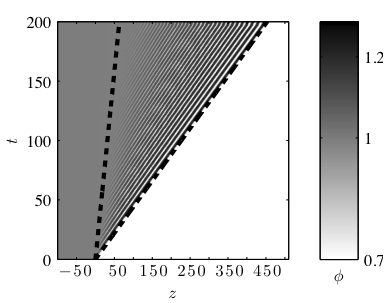
(a) $(n,m)=(3,0),\phi_{+}=0.7$

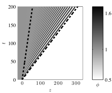
(b) $(n,m)=(2,1),\phi_{+}=0.5$

Figure 6: Contour plots of numerical solutions for $\phi(z,t)$ plotted in the characteristic $z$-$t$ plane for different parameter values with the overlying dashed lines indicating the predicted values for the leading and trailing edge speeds. The angles (speeds) line up excellently.

5.2 Breakdown of Analytical Method

The Whitham-El DSW simple wave closure method used here requires the existence of a self-similar simple wave solution to the full set of the Whitham modulation equations. In this section, we identify two mechanisms that lead to the breakdown of this simple wave theory, the onset of linear degeneracy or zero dispersion. In the former case, a loss of monotonicity manifests such that the simple wave can no longer be continued. For the latter case, zero dispersion corresponds to a gradient catastophe in the Whitham modulation equations leading to compression and implosion of the DSW.

First we consider the zero dispersion case at the trailing edge. The right eigenvector of the system (36), (37) associated with the characteristic speed $\frac{\partial}{\partial k}\omega_{0}$ of the trailing edge is $[0,1]^{\mathrm{T}}$. Therefore, in the vicinity of the trailing edge, the self-similar simple wave satisfies

$$\bar{\phi}^{\prime}=0,\quad k^{\prime}=\left(\frac{\partial^{2}\omega_{0}}{\partial k^{2}}\right)^{-1}{\rm Phys.~{}Rev.~{}D}$$

Hence, if $\frac{\partial^{2}}{\partial k^{2}}\omega_{0}(k,1)\rightarrow 0$ for $k$ near $k_{-}$, gradient catastrophe in the modulation system is experienced. This condition corresponds to a change in the sign of dispersion and is equivalent to the loss of genuine nonlinearity in the trailing edge system itself. As we will show later, this is distinct from the loss of genuine nonlinearity of the full Whitham modulation system, in the limit of the trailing edge. Recalling that the sign of dispersion changes when $k^{2}=3\Phi^{m-n}$ (see eq. (17)), we have the criterion $k_{-}\geq\sqrt{3}$ leading to gradient catastrophe. More generally, for any simple wave, one-phase DSW resulting from step-like initial data of a scalar, dispersive, nonlinear wave equation for $\phi$, we can formulate the following condition which must hold for the assumption of a continuously expanding, one-phase region:

$$\left.\frac{\partial^{2}}{\partial k^{2}}\omega_{0}(k,\bar{\phi})\right|_{(k_{-},\phi_{-})}<0.$$ (66)

The criterion (66) holds for systems with negative dispersion in the long wavelength regime, the inequality reversed for the positive dispersion case. This is a natural generalization of the criterion in modulated linear wave theory where a change in the sign of dispersion is associated with the formation of caustics and break down of the leading order stationary phase method (Ostrovsky & Potapov, 2002). It is notable that Whitham hypothesized that breaking of the modulation equations could lead to an additional source of oscillations (see Section 15.4 in Whitham (1974)). Previous works have resolved breaking in the Whitham equations by considering modulated multiphase waves in the context of DSW interactions (Grava & Tian, 2002; Hoefer & Ablowitz, 2007; Ablowitz et al., 2009) or in the context of certain initial value problems (Jorge et al., 1999). Beginning with the initial, groundbreaking work (Flashka et al., 1980) on multiphase Whitham averaging for KdV, all studies since have involved integrable systems. Since $k_{-}$ is a monotonically decreasing function of $\phi_{+}$ for the magma DSW, we expect gradient catastrophe and DSW implosion for sufficiently large jumps, i.e. $\phi_{+}<\phi_{\mathrm{c}}$ for the critical jump height $\phi_{\mathrm{c}}$. Using our work in Section 4, we can derive $\phi_{\mathrm{c}}$ for which we violate (66). We note the following

$$\frac{\mathrm{d}}{\mathrm{d}\phi_{+}}\left[\frac{\partial}{\partial k}\omega_{0}(k_{-},1)\right]=-\left(\frac{\partial^{2}}{\partial k^{2}}\omega_{0}(k_{-},1)\right)k^{\prime}(1).$$ (67)

The trailing edge wavenumber $k_{-}=k(1)$ depends on $\phi_{+}$ through the initial condition $k(\phi_{+})=0$ (recall eq. (40)). Therefore, in eq. (67), $\mathrm{d}k_{-}/\mathrm{d}\phi_{+}=-k^{\prime}(1)$. Hence, the change in sign of dispersion evaluated at the trailing edge coincides with a minimum of the linear edge speed as a function of $\phi_{+}$ (see figures 3(a) and 3(b)). The dispersion sign changes from negative to positive when $\phi_{+}=\phi_{\mathrm{c}}=\phi_{\mathrm{min}}$, where $\phi_{\mathrm{min}}$ is given in eq. (65). Our analytical method then is no longer valid for jumps larger than this threshold value. This coincidence of a global minimum edge speed and breakdown of the analytical method was also noted in the case of unsteady, undular bores in shallow-water by El et al. (2006), however the mechanism was argued to be due to the loss of genuine nonlinearity in the modulation system. The sign of dispersion did not change.

A similar argument holds in the vicinity of the leading edge. There, gradient catastrophe occurs if the conjugate phase velocity (i.e. the speed of the leading edge) increases with decreasing $\tilde{k}$. Then one-phase behavior is expected to be retained when

$$\left.\frac{\partial}{\partial\tilde{k}}\left(\frac{\tilde{\omega}_{\mathrm{s}}}{\tilde{k}}\right)\right|_{(\tilde{k}_{+},\phi_{+})}>0{\rm Phys.~{}Rev.~{}D}$$ (68)

The condition (66) says that the sign of dispersion must remain negative when evaluated at the trailing edge. The second condition (68) requires that the sign of the conjugate dispersion (now defined through changes in the phase velocity) remain positive when evaluated at the leading edge. Verifying (68), we find that it does indeed hold for every $\phi_{+}\in(0,1)$.

The simple wave construction also requires that the full modulation system be strictly hyperbolic and genuinely nonlinear. Strict hyperbolicity of the full modulation system requires the three characteristics be real and distinct at all points except at the DSW boundaries which correspond to the merger of two characteristics. In integrable systems, this can be validated directly due to the availability of Riemann invariants, but in the non-integrable case we assume strict hyperbolicity. Genuine nonlinearity, on the other hand, is a condition necessary for the construction of the integral curve connecting the leading and trailing edges and requires that the characteristic speed $\lambda$ varies monotonically along the integral curve. Again, we cannot check this condition for all parameters in the full modulation system, but we can in neighborhoods near the boundaries. Parameterizing the integral curve by $\bar{\phi}$, the monotonicity criteria are

$$\left.\frac{\mathrm{d}\lambda}{\mathrm{d}\bar{\phi}}\right|_{(k=k_{-},\bar{\phi}=1,a=0)}=\left.\frac{\partial\lambda}{\partial k}k^{\prime}+\frac{\partial\lambda}{\partial\bar{\phi}}+\frac{\partial\lambda}{\partial a}\frac{\mathrm{d}a}{\mathrm{d}\bar{\phi}}\right|_{(k=k_{-},\bar{\phi}=1,a=0)}<0,$$ (69)

$$\left.\frac{\mathrm{d}\lambda}{\mathrm{d}\bar{\phi}}\right|_{(\tilde{k}=\tilde{k}_{+},\bar{\phi}=\phi_{+},\Lambda=0)}=\left.\frac{\partial\lambda}{\partial\tilde{k}}\tilde{k}^{\prime}+\frac{\partial\lambda}{\partial\bar{\phi}}+\frac{\partial\lambda}{\partial\Lambda}\frac{\mathrm{d}\Lambda}{\mathrm{d}\bar{\phi}}\right|_{(\tilde{k}=\tilde{k}_{+},\bar{\phi}=\phi_{+},\Lambda=0)}>0{\rm Phys.~{}Rev.~{}D}$$ (70)

These monotonicity conditions are the correct way to determine genuine nonlinearity at the trailing and leading edges. Testing for genuine nonlinearity in the reduced system of two modulations equations fails to provide the proper condition (recall eq. (66)) because they are restricted to the $a=0$ plane. Since the trailing and leading edges correspond to double characteristics, right and left differentiability, respectively, imply $\frac{\partial\lambda}{\partial a}\rightarrow 0$ and $\frac{\partial\lambda}{\partial\Lambda}\rightarrow 0$ at the appropriate edge. Also, the limiting characteristic speeds are $\lambda\rightarrow\frac{\partial}{\partial k}\omega_{0}$ and $\lambda\rightarrow\frac{\tilde{\omega}}{\tilde{k}}$ at the trailing and leading edges, respectively. Then the monotonicity criteria (69) and (70), after the change of variables to $\alpha$ and $\tilde{\alpha}$, simplify to

$$\begin{split}\left.\frac{\mathrm{d}\lambda}{\mathrm{d}\bar{\phi}}\right|_{(k=k_{-},\bar{\phi}=1,a=0)}&=\left.\frac{\frac{\partial^{2}}{\partial k^{2}}\omega_{0}\frac{\partial}{\partial\bar{\phi}}\omega_{0}}{n\bar{\phi}^{n-1}-\frac{\partial}{\partial k}\omega_{0}}+\frac{\partial^{2}\omega_{0}}{\partial k\partial\bar{\phi}}\right|_{(k=k_{-},\bar{\phi}=\phi_{-},a=0)}\\ &=-\frac{n\alpha_{-}\left(16\alpha_{-}^{3}m-(16m+4)\alpha_{-}^{2}+(3n-m+2)\alpha_{-}+m-1\right)}{2\alpha_{-}+1}<0,\end{split}$$ (71)

$$\begin{split}\left.\frac{\mathrm{d}\lambda}{\mathrm{d}\bar{\phi}}\right|_{(\tilde{k}=\tilde{k}_{+},\bar{\phi}=\phi_{+},\Lambda=0)}&=\left.\frac{\frac{\partial}{\partial\bar{\phi}}\tilde{\omega}_{0}(\tilde{k}n\bar{\phi}^{n-1}-\tilde{\omega}_{0})}{\tilde{k}^{2}\left(n\bar{\phi}^{n-1}-\frac{\partial}{\partial\tilde{k}}\tilde{\omega}_{0}\right)}\right|_{(\tilde{k}=\tilde{k}_{+},\bar{\phi}=\phi_{+},\Lambda=0)}\\ &=\frac{\phi_{+}^{n-2}n\tilde{\alpha}\left(4\tilde{\alpha}^{2}+(n-m+4)\tilde{\alpha}+m-1\right)}{2\tilde{\alpha}+1}>0{\rm Phys.~{}Rev.~{}D}\end{split}$$ (72)

When either of these two conditions is not satisfied, a breakdown in genuine nonlinearity of the full $3\times 3$ modulation system occurs at the boundaries, (71) and (72) corresponding to the trailing, linear edge and the leading solitary wave edge, respectively. We can verify analytically that for any value of $\phi_{+}\in(0,1)$ and for all $(n,m)$ in the physical range, condition (72) is satisfied. For the linear edge condition (71), however, we can derive a condition for $\phi_{+}$ such that the monotonicity condition is broken. Linear degeneracy first occurs when $\alpha=\alpha_{\mathrm{l}}$, where $\alpha_{\mathrm{l}}$ satisfies

$$16m\alpha_{\mathrm{l}}^{3}-(16m+4)\alpha_{\mathrm{l}}^{2}+(3n-m+2)\alpha_{\mathrm{l}}+m-1=0{\rm Phys.~{}Rev.~{}D}$$ (73)

From the IVP (43) and the implicit relation between $\alpha$ and $\bar{\phi}$ (45), we know that if there exists an $\alpha_{\mathrm{l}}\in(0,1]$ which satisfies (73), then we can find $\phi_{+}=\phi_{\mathrm{l}}$ such that (71) is no longer satisfied. Then for each $(n,m)$ in the physical range, there is a critical jump height $\phi_{\mathrm{l}}$ such that genuine nonlinearity is lost at the trailing edge. Note that for $m=1$, $\alpha_{\mathrm{l}}=0$ is the only root of eq. (73) in the valid range and this gives the value $\phi_{\mathrm{l}}=0$ which is outside the range of interest. We have verified numerically that $\phi_{\mathrm{c}}>\phi_{\mathrm{l}}$ for all $n\in[2,5]$, $m\in[0,1]$ so implosion occurs before the loss of genuine nonlinearity. Before linear degeneracy occurs, the analytical construction has already broken down due to a change in sign of dispersion (66). We have found three distinguished jump heights exhibiting the ordering $\phi_{\mathrm{b}}>\phi_{\mathrm{c}}>\phi_{\mathrm{l}}$. As $\phi_{+}$ is decreased through these values, the DSW exhibits backflow and then implosion before it ever reaches linear degeneracy.

Figure 7 shows the key results of our analysis. Plots of the numerically computed solutions for the two parameter cases tested in the regimes $\phi_{+}\in\left\{(\phi_{\mathrm{b}},1),(\phi_{\mathrm{c}},\phi_{\mathrm{b}}),(0,\phi_{\mathrm{c}})\right\}$ are shown. We see in both cases that our analytical predictions for $\phi_{\mathrm{b}}$ and $\phi_{\mathrm{c}}$ are in agreement with the numerical solution as backflow and DSW implosion occur when expected and not otherwise. The choices for $\phi_{+}$ in figure 7 were chosen for visual clarity but we have performed further simulations with $\phi_{+}$ much closer to $\phi_{\mathrm{b}}$ and $\phi_{\mathrm{c}}$, finding that they do indeed accurately predict the transitions in DSW behavior. For $\phi_{+}<\phi_{\mathrm{c}}$, the DSW rank-ordering breaks down due to catastrophe and results in wave interactions in the interior of the oscillatory region. In figure 8 we show an example of how the solution evolves from step initial data for $\phi_{+}<\phi_{\mathrm{c}}$. The interior of the DSW initially develops into approximately a modulated one-phase region. However, as the simulation continues, the trailing edge linear waves stagnate due to the minimum in the group velocity. The DSW is compressed as shorter waves at the leftmost edge are overtaken by longer waves from the interior. Wave interactions in the DSW interior ensue. Another one-phase region develops, separated from the main trunk of the DSW by a two-phase region, further clarified by the contour plot of $\phi$ in the characteristic $z$-$t$ plane in figure 9. We find that the closer $\phi_{+}$ is to $\phi_{\mathrm{c}}$, the longer it takes for the interaction region to develop from step initial data.

This analysis suggests not only that our analytical construction accurately captures physically important, critical values in $\phi_{+}$, but also that our predictions of the trailing edge speed $s_{-}$ from Section 4.2 are consistent with the numerical simulations.

(a) $(n,m)=(3,0)$

(b) $(n,m)=(2,1)$

Figure 7: From top to bottom, magma DSWs in the forward propagating case, the backflow regime before gradient catastrophe, and after DSW implosion. The solutions shown correspond, from top to bottom, to (a) $t_{\mathrm{f}}=\left\{200,150,150\right\}$, (b) $t_{\mathrm{f}}=\left\{400,200,200\right\}$.

Figure 8: DSW implosion. Evolution of the solution to eq. (1) with $(n,m)=(2,1)$, $\phi_{+}=.1<\phi_{\mathrm{c}}\approx 0.16$. The solution initially develops into a typical DSW with one-phase interior, but as it evolves, the trailing edge compresses and longer waves from the interior overtake shorter waves near the edge. Internal wave interactions (implosion) commence and the one-phase assumption is no longer valid.

Figure 9: Contour plot of numerically computed $\phi(z,t)$ from figure 8 in the characteristic $z$-$t$ plane exhibiting modulated one-phase and two-phase behavior.

6 Summary and Conclusions

In summary, we have analytically determined DSW speeds and amplitudes for arbitrary initial jumps and for physical values of the constitutive parameters. It is likely that these results extend directly to non-physical parameter values as well. In figure 7, we see backflow and DSW implosion for jumps beyond the catastrophe point $\phi_{\mathrm{c}}$, revealing internal wave interactions and the need for modification of the one-phase region ansatz in the description of the DSW. Direct analysis of the full Whitham system would be required for further study, a highly nontrivial task for arbitrary $(n,m)$. The significance of this work is its characterization of magma DSW solutions, an open problem since observed in Spiegelman (1993b), its generalization to include the effects of bulk viscosity on porosity oscillations, and, more generally in the field of dispersive hydrodynamics, the new DSW dynamics predicted and observed. A regime which remains to be understood is the flow of a magma into a “dry” region, i.e. $\phi\rightarrow 0$. The original paper Spiegelman (1993b) conjectured that the leading solitary wave would take on unbounded amplitude, implying physical disaggregation of the multiphase medium. This paper has not explored the behavior of solutions as the jump approaches this singular limit, and a viable alternative approach is yet to be proposed.

Aside from the novelty of dispersive shock behavior in viscously dominated fluids, this work provides the theoretical basis with which to experimentally study DSW generation. Solitary waves in the fluid conduit system have been carefully studied experimentally (Scott et al., 1986; Olson & Christensen, 1986; Helfrich & Whitehead, 1990), showing good agreement with the soliton amplitude/speed relation (28) in the weak to moderate jump regime. DSW speeds, the lead solitary wave amplitue, and the onset of backflow are all experimentally testable predictions. Furthermore, the ability to carefully measure DSW properties in this system would enable the first quantitative comparison of non-integrable Whitham theory with experiment, previous comparisons being limited to qualitative features (Hoefer et al., 2006; Wan et al., 2007; Conti et al., 2009) or the weakly nonlinear, KdV regime for plasma (Tran et al., 1977) and the weakly nonlinear, Benjamin-Ono equation for atmospheric phenomena (Porter & Smyth, 2002). Due to its experimental relevance, the viscous fluid conduit system deserves further theoretical study in the large amplitude regime. What are the limits of applicability of the magma equation to this system? How do higher order corrections affect the dynamics?

Finally, we have established new, testable criteria for the breakdown of the DSW solution method in equations (66), (68), (69), and (70). The additional four admissibility criteria–loss of genuine nonlinearity, change in sign of dispersion at the solitary wave, linear wave edges–apply to the simple wave DSW construction of any nonlinear dispersive wave problem. Linear degeneracy and nonstrict hyperbolicity have been accommodated in various integrable nonlinear wave problems (Pierce & Tian, 2007; Kodama et al., 2008; Kamchatnov et al., 2012). Extensions to non-integrable problems are needed.

We thank Marc Spiegelman for introducing us to the magma equation and for many helpful suggestions and fruitful discussion. We appreciate thoughtful comments from Noel Smyth. This work was supported by NSF Grant Nos. DGE–1252376 and DMS–1008973.

Appendix A Numerical method

The magma equation was simulated using a sixth-order finite difference spatial discretization with explicit Runge-Kutta time stepping. The initial condition (39) was approximated by a smoothed step function centered at $z=0$

$$\phi(z,0)=\frac{1}{2}\left[\left(1+\phi_{+}\right)+\left(\phi_{+}-1\right)\tanh\left({\frac{z}{4\lambda}}\right)\right],$$ (74)

where $\phi$ is the porosity and we assume $\phi(z,t)>0$ and $\phi_{+}\in(0,1)$. The width $\lambda$ was chosen to be sufficiently large in comparison with the spatial grid spacing, typically $\lambda=10\Delta z$ for grid spacing $\Delta z$. This is reasonable since we are concerned with the long-time asymptotic behavior of the solution and any effects of the initial profile’s transients will be negligible. We choose a truncated spatial domain wide enough in order to avoid wave reflections at the boundary. It is also convenient to consider the magma equation in the form (8), (9). In this form, we have an ODE coupled to a linear elliptic operator $L(\phi)\mathcal{P}=-(\phi^{n})_{z}$. We first solve for $\mathcal{P}$ by discretizing and inverting $L(\phi)$ using sixth-order, centered differences. To obtain boundary conditions, we note $\mathcal{P}=\phi^{-m}\phi_{t}$, and due to the wide domain, the function $\phi$ assumes a constant value at the boundaries so $\mathcal{P}$ decays to zero near the boundaries. Hence we implement Dirichlet boundary conditions on the compaction pressure. We then use the solution for $\mathcal{P}$ to update the righthand side of eq. (8) and step forward in time using the classical, explicit 4th order Runge-Kutta method. The temporal grid spacing was chosen to satisfy the Courant$-$Friedrichs$-$Lewy (CFL) condition for the dispersionless limit, $\frac{\Delta t}{\Delta z}\leq\frac{1}{n}$. Typically, we took $\Delta t=\frac{\Delta z}{2n}$.

The accuracy of our numerical scheme has been determined by simulating solitary wave solutions on a background porosity $\phi=1$ as derived by Nakayama & Mason (1992), for the particular parameter regimes $(n,m)\in\{(2,1),(3,0)\}$, used in our analysis. We numerically solve for $\phi$ from the nonlinear traveling wave equation $(\phi^{\prime})^{2}=g(\phi)$, i.e. eq. (24) with $\phi_{2}\rightarrow\phi_{1}$, and use this as our initial profile. The $\infty$-norm difference between the numerically propagated solution $\phi^{*}$ and the true solitary wave solution $\phi$ is our figure of merit.

To compute the initial solitary wave profile, we implicitly evaluate

$$z-ct=I=\int_{\phi}^{A}\frac{\mathrm{d}\tilde{u}}{\sqrt{g(\tilde{u})}},\quad z\leq 0$$ (75)

where $A$ is the peak height of the solitary wave, and $\phi>1$. We then perform an even reflection about the solitary wave center. The difficulty in evaluation of (75) arises from the square root singularity in the integrand when $\tilde{u}=A$ and the logarithmic singularity when $\tilde{u}$ is near one. We deal with this by breaking up the integral around these singular points as

$$I=I_{1}+I_{2}+I_{3}$$ (76)

where

$$I_{1}=\int_{\phi}^{\phi+\mu}\frac{\mathrm{d}\tilde{u}}{\sqrt{g(\tilde{u})}},\quad I_{2}=\int_{\phi+\mu}^{A-\varepsilon}\frac{\mathrm{d}\tilde{u}}{\sqrt{g(\tilde{u})}},\quad I_{3}=\int_{A-\varepsilon}^{A}\frac{\mathrm{d}\tilde{u}}{\sqrt{g(\tilde{u})}},$$ (77)

and $\mu>0,\varepsilon>0$ are small and to be chosen. We evaluate $I_{1}$ and $I_{3}$ using Taylor expansions up to first order and calculate $I_{2}$ via standard numerical quadrature. The parameters $\mu$ and $\varepsilon$ are chosen so that the approximate error in evaluation of $I_{1}$, $I_{2}$, and $I_{3}$ are less than some desired level of tolerance, tol. Errors in $I_{1}$ and $I_{3}$ are due to the local Taylor expansion near the singularities. The errors in $I_{2}$ are due to the loss of significant digits in floating point arithmetic.

For $0<\tilde{u}+\mu-1\ll 1$, the approximate rounding error in $I_{2}$ is

$$fl(\frac{1}{\sqrt{g(\tilde{u}+\mu)}})\approx(\frac{1}{2}g^{\prime\prime}(1))^{-\frac{1}{2}}(\tilde{u}+\mu-1+\varepsilon_{\mathrm{mach}})^{-1},$$ (78)

where $fl(x)$ represents the evaluation of $x$ in floating point arithmetic and $\varepsilon_{\mathrm{mach}}$ is machine precision ($\approx 2.2\times 10^{-16}$ in double precision). To constrain the error so that it is less than tol, we require

$$\mu>\left(\frac{\varepsilon_{\text{mach}}}{\texttt{tol}\left(2g^{\prime\prime}(1)\right)^{\frac{1}{2}}}\right)^{\frac{1}{2}}-\tilde{u}-1,$$ (79)

and

$$\varepsilon>\frac{A\ \varepsilon_{\text{mach}}}{2\left(-g^{\prime}(A)\right)^{\frac{1}{2}}\texttt{tol}}{\rm Phys.~{}Rev.~{}D}$$ (80)

To evaluate $I_{1}$, we utilize a first order Taylor expansion of $g(\tilde{u})$ near $\tilde{u}=1$, which gives

$$I_{1}\approx\left(\frac{1}{2}g^{\prime\prime}\left(1\right)\right)^{-\frac{1}{2}}\left[\ln{\left(\frac{\tilde{u}+\mu-1}{\tilde{u}-1}\right)}-\frac{\mu g^{\prime\prime\prime}(1)}{6g^{\prime\prime}(1)}\right]{\rm Phys.~{}Rev.~{}D}$$ (81)

Then if we take the second term to be the approximate error and require it be less in magnitude than tol, we find a second restriction on $\mu$

$$\mu<\frac{6\sqrt{2}\left|g^{\prime\prime}(1)\right|^{\frac{3}{2}}\texttt{tol}}{\left|g^{\prime\prime\prime}(1)\right|}{\rm Phys.~{}Rev.~{}D}$$ (82)

A similar procedure for $I_{3}$ leads to

$$\varepsilon<\left(\frac{6(-g^{\prime}(A))\texttt{tol}}{g^{\prime\prime}(A)}\right)^{\frac{2}{3}}{\rm Phys.~{}Rev.~{}D}$$ (83)

Hence, we choose $\varepsilon$ and $\mu$ such that

$$\varepsilon=\frac{A\ \varepsilon_{\text{mach}}}{2\left(-g^{\prime}(A)\right)^{\frac{1}{2}}\texttt{tol}},$$ (84)

and

$$\mu=\max\left\{0,\left(\frac{\varepsilon_{\text{mach}}}{\texttt{tol}\left(2g^{\prime\prime}(1)\right)^{\frac{1}{2}}}\right)^{\frac{1}{2}}-u-1\right\}{\rm Phys.~{}Rev.~{}D}$$ (85)

We chose $\texttt{tol}=10^{-7}$ and found this to give a sufficiently accurate solitary wave profile. Using this as an initial condition, we initiate our magma equation solver for a solitary wave of height twice the background and a time evolution of approximately 10 dimensionless units. We ran successive simulations for a range of decreasing $\Delta z$ values and $\Delta t$ chosen as described above (note that simulations of fixed $\Delta z$ and a variable $\Delta t$ showed that the spatial grid was the dominant source of numerical error). The convergence of the numerical error is described by figure 10, where the solution converges at sixth order as expected. Note that there is an alternative method for numerically calculating solitary wave solutions to eq. (1) for arbitrary $n,m$ in all dimensions (Simpson & Spiegelman, 2011).

Based on these solitary wave validation studies, we typically use the conservative value $\Delta z=0.05$, though coarser grids were taken in small amplitude cases where the solutions exhibited longer wavelength oscillations and had to propagate for much longer times. The final time $t_{\mathrm{f}}$ depended upon the jump $\phi_{+}$, with $t_{\mathrm{f}}$ typically at least 1000 for smaller jumps and $t_{\mathrm{f}}\approx 200$ for larger jumps.

(a) $(n,m)=(3,0)$

(b) $(n,m)=(2,1)$

Figure 10: Convergence plots of the $\infty$-norm of the difference of the numerically evolved solitary wave versus the true solution. In both cases, the time discretization $\Delta t$ is fixed and we vary $\Delta z$. The dotted lines indicate the desired sixth order convergence.

To calculate the leading edge speed $s_{+}$ and its amplitude $a_{+}$, we generally consider the long time numerical simulations for the last two dimensionless units of time. We then find the maximum at each fixed time and locally interpolate the discrete porosity function on a grid with spacing $10^{-4}\Delta z$. This ensures we find the “true” numerical maximum and not just the highest point on the grid. We then recompute the maximum of the interpolated porosities, and the value at the final time is the amplitude $a_{+}$. To find $s_{+}$, we compute the slope of the least squares linear fit to the function connecting the positions of the interpolated porosity maxima versus their respective times. This is the leading edge speed.

References

- Ablowitz et al. (2009) Ablowitz, M. J., Baldwin, D. E. & Hoefer, M. A. 2009 Soliton generation and multiple phases in dispersive shock and rarefaction wave interaction. Phys. Rev. E 80, 016603.
- Barcilon & Lovera (1989) Barcilon, V. & Lovera, O. M. 1989 Solitary waves in magma dynamics. J. Fluid Mech. 204, 121–133.
- Barcilon & Richter (1986) Barcilon, V. & Richter, F. M. 1986 Nonlinear waves in compacting media. J. Fluid Mech. 164, 429–448.
- Chanson (2010) Chanson, H. 2010 Tidal bores, aegir and pororoca: The geophysical wonders. World Scientific.
- Conti et al. (2009) Conti, C., Fratalocchi, A., Peccianti, M., Ruocco, G. & Trillo, S. 2009 Observation of a gradient catastrophe generating solitons. Phys. Rev. Lett. 102, 083902.
- Dutton et al. (2001) Dutton, Z., Budde, M., Slowe, C. & Hau, L. V. 2001 Observation of quantum shock waves created with ultra-compressed slow light pulses in a Bose-Einstein condensate. Science 293, 663.
- El (2005) El, G. A. 2005 Resolution of a shock in hyperbolic systems modified by weak dispersion. Chaos 15, 037103.
- El et al. (2006) El, G. A., Grimshaw, R. H. J. & Smyth, N. F. 2006 Unsteady undular bores in fully nonlinear shallow-water theory. Phys. Fluids 18, 027104.
- El et al. (2009) El, G. A., Grimshaw, R. H. J. & Smyth, N. F. 2009 Transcritical shallow-water flow past topography: finite-amplitude theory. J. Fluid Mech. 640, 187.
- Elperin et al. (1994) Elperin, T., Kleeorin, N. & Krylov, A. 1994 Nondissipative shock waves in two-phase flows. Physica D 74, 372–385.
- Esler & Pearce (2011) Esler, J. G. & Pearce, J. D. 2011 Dispersive dam-break and lock-exchange flows in a two-layer fluid. J. Fluid Mech. 667, 555–585.
- Flashka et al. (1980) Flashka, H., Forest, M. G. & McLaughlin, D. W. 1980 Multiphase averaging and the inverse spectral transform of the Korteweg–de Vries equation. Comm. Pure Appl. Math. 33, 739–784.
- Fowler (1985) Fowler, A. C. 1985 A mathematical model of magma transport in the asthenosphere. Geophys. Astrophys. Fluid Dynamics pp. 63–96.
- Grava & Tian (2002) Grava, T. & Tian, F.-R. 2002 The generation, propagation, and extinction of multiphases in the KdV zero-dispersion limit. Comm. Pur. Appl. Math. 55, 1569–1639.
- Gurevich & Pitaevskii (1974) Gurevich, A. V. & Pitaevskii, L. P. 1974 Nonstationary structure of a collissionless shock wave. Sov. Phys. JETP 33, 291–297.
- Harris (1996) Harris, S. E. 1996 Conservation laws for a nonlinear wave equation. Nonlinearity 9, 187–208.
- Harris & Clarkson (2006) Harris, S. E. & Clarkson, P. A. 2006 Painleve analysis and similarity reductions for the magma equation. SIGMA 2, 68.
- Helfrich & Whitehead (1990) Helfrich, K. R. & Whitehead, J. A. 1990 Solitary waves on conduits of buoyant fluid in a more viscous fluid. Geophys. Astro. Fluid 51, 35–52.
- Hoefer & Ablowitz (2007) Hoefer, M. A. & Ablowitz, M. J. 2007 Interactions of dispersive shock waves. Physica D 236, 44–64.
- Hoefer et al. (2006) Hoefer, M. A., Ablowitz, M. J., Coddington, I., Cornell, E. A., Engels, P. & Schweikhard, V. 2006 Dispersive and classical shock waves in Bose-Einstein condensates and gas dynamics. Phys. Rev. A 74, 023623.
- Jorge et al. (1999) Jorge, M. C., Minzoni, A. A. & Smyth, N. F. 1999 Modulation solutions for the Benjamin–Ono equation. Physica D 132, 1–18.
- Kamchatnov et al. (2012) Kamchatnov, A. M., Kuo, Y. H., Lin, T. C., Horng, T. L., Gou, S. C., Clift, R., El, G. A. & Grimshaw, R. H. J. 2012 Undular bore theory for the Gardner equation. Phys. Rev. E 86, 036605.
- Katz et al. (2007) Katz, R. F., Knepley, M., Smith, B., Spiegelman, M. & Coon, E. 2007 Numerical simulation of geodynamic processes with the Portable Extensible Toolkit for Scientific Computation. Phys. Earth Planet Int. 163, 52–68.
- Kodama et al. (2008) Kodama, Y., Pierce, V. U. & Tian, F.-R. 2008 On the Whitham equations for the defocusing complex modified KdV equation. SIAM J. Math. Anal. 41, 26–58.
- Marchant & Smyth (2005) Marchant, T. R. & Smyth, N. F. 2005 Approximate solutions for magmon propagation from a reservoir. IMA J. Appl. Math 70, 793–813.
- McKenzie (1984) McKenzie, D. 1984 The generation and compaction of partially molten rock. J. Petrol. 25, 713–765.
- Nakayama & Mason (1992) Nakayama, M. & Mason, D. P. 1992 Rarefactive solitary waves in two-phase fluid flow of compacting media. Wave Motion 15, 357–392.
- Olson & Christensen (1986) Olson, P. & Christensen, U. 1986 Solitary wave propagation in a fluid conduit within a viscous matrix. J. Geophys. Res. 91, 6367–6374.
- Ostrovsky & Potapov (2002) Ostrovsky, L. A. & Potapov, A. I. 2002 Modulated waves: Theory and applications. Johns Hopkins University Press.
- Pierce & Tian (2007) Pierce, V. U. & Tian, F.-R. 2007 Self-similar solutions of the non-strictly hyperbolic Whitham equations for the KdV hierarchy. Dyn. PDE 4, 263–282.
- Porter & Smyth (2002) Porter, V. A. & Smyth, N. F. 2002 Modeling the Morning Glory of the Gulf of Carpentia. J. Fluid Mech. 454, 1–20.
- Richter & McKenzie (1984) Richter, F. M. & McKenzie, D. 1984 Dynamical models for melt segregation from a deformable matrix. J. Geol. 92, 729–740.
- Scheidegger (1974) Scheidegger, A. E. 1974 The physics of flow through porous media. University of Toronto Press.
- Scott & Stevenson (1984) Scott, D. R. & Stevenson, D. J. 1984 Magma solitons. Geophys. Res. Lett. 11, 1161–1164.
- Scott & Stevenson (1986) Scott, D. R. & Stevenson, D. J. 1986 Magma ascent by porous flow. Geophys. Res. Lett. 91, 9283–9296.
- Scott et al. (1986) Scott, D. R., Stevenson, D. J. & Whitehead, J. A. 1986 Observations of solitary waves in a viscously deformable pipe. Nature 319, 759–761.
- Simpson & Spiegelman (2011) Simpson, G. & Spiegelman, M. 2011 Solitary wave benchmarks in magma dynamics. J. Sci. Comput. 49, 268–290.
- Simpson et al. (2007) Simpson, G., Spiegelman, M. & Weinstein, M. I. 2007 Degenerate dispersive equations arising in the study of magma dynamics. Nonlinearity 20.
- Simpson et al. (2010) Simpson, G., Spiegelman, M. & Weinstein, M. I. 2010 A multiscale model of partial melts I: Effective equations. J. Geophys. Res.–Sol. Ea. 115, B04410.
- Simpson & Weinstein (2008) Simpson, G & Weinstein, M. I. 2008 Asymptotic stability of ascending solitary magma waves. SIAM J. Math. Anal. 40, 1337–1391.
- Spiegelman (1993a) Spiegelman, M 1993a Flow in deformable porous media I. simple analysis. J. Fluid Mech. 247, 17–38.
- Spiegelman (1993b) Spiegelman, M. 1993b Flow in deformable porous media II. numerical analysis–the relationship between shock waves and solitary waves. J. Fluid Mech. 247, 39–63.
- Spiegelman et al. (2001) Spiegelman, M., Kelemen, P. B. & Aharonov, E. 2001 Causes and consequences of flow organization during melt transport: The reaction infiltration instability in compactible media. J. Geophys. Res. 106, 2061–2077.
- Takahashi et al. (1990) Takahashi, D., Sachs, J. R. & Satsuma, J. 1990 Properties of the magma and modified magma equations. J. Phys. Soc. of Jap. 59, 1941–1953.
- Taylor et al. (1970) Taylor, R. J., Baker, D. R. & Ikezi, H. 1970 Observation of collisionless electrostatic shocks. Phys. Rev. Lett. 24, 206–209.
- Tran et al. (1977) Tran, M. Q., Appert, K., Hollenstein, C., Means, R. W. & Vaclavik, J. 1977 Shocklike solutions of the Korteweg-de Vries equation. Plasma Physics 19, 381.
- Wan et al. (2007) Wan, W., Jia, S. & Fleischer, J. W. 2007 Dispersive superfluid-like shock waves in nonlinear optics. Nat. Phys. 3, 46–51.
- Whitehead & Helfrich (1986) Whitehead, J. A. & Helfrich, K. R. 1986 The Korteweg–deVries equation from laboratory conduit and magma migration equations. Geophys. Res. Lett. 13, 545–546.
- Whitham (1965) Whitham, G. B. 1965 Non-linear dispersive waves. Proc. R. Soc. Lond., Ser. A 283, 238–261.
- Whitham (1974) Whitham, G. B. 1974 Linear and nonlinear waves. Wiley and Sons.