Dynamical local and non-local Casimir atomic phases

Abstract

We develop an open-system dynamical theory of the Casimir interaction between coherent atomic waves and a material surface. The system — the external atomic waves — disturbs the environment — the electromagnetic field and the atomic dipole degrees of freedom — in a non- local manner by leaving footprints on distinct paths of the atom interferometer. This induces a non-local dynamical phase depending simultaneously on two distinct paths, beyond usual atom-optics methods, and comparable to the local dynamical phase corrections. Non-local and local atomic phase coherences are thus equally important to capture the interplay between the external atomic motion and the Casimir interaction. Such dynamical phases are obtained for finite-width wavepackets by developing a diagrammatic expansion of the disturbed environment quantum state.

I INTRODUCTION

The interplay between the internal atomic dynamics and the electromagnetic (EM) field retardation, brought to light by the pioneering work of Casimir and Polder CasimirPolder , is crucial to understand the atom-surface dispersive interaction in the long-distance limit (see Intravaia for a recent review). In contrast, the effect of the external atomic motion on the dispersive interaction is almost always discarded. Notable exceptions are the quantum friction effects resulting from the shear relative motion between two material surfaces  QuantumFrictionPP or between an atom and a surface QuantumFrictionAP ; Scheel09 .

Since the usual atomic velocities are strongly non-relativistic, one might expect the dynamical corrections to the dispersive atom-surface interaction to be very small. Because of their high sensitivity, atom interferometers Cronin09 ; Kasevich07 are ideal systems for probing such small corrections. There is a growing interest in developing atom interferometers able to probe surface interactions. Measurements of the van der Waals atom-surface interaction with standard atom interferometry have already been achieved Cronin04 ; CroninVigue ; Lepoutre11 , while optical-lattice atom interferometry offers even more promising perspectives to measure the Casimir-Polder interaction in the long-distance regime FORCAGpapers .

From a fundamental point of view, the coherent atomic waves evolving in the vicinity of a material surface constitute a particularly rich open quantum system: the external atomic waves, playing the role of the system, interact with an environment involving both long-lived (atomic dipole) and short-lived (EM field) degrees of freedom (dofs). In this paper, we develop an open-system theory of atom interferometers in the vicinity of a material surface. We show that the atomic motion relative to the surface along the interferometer paths gives rise to a non-local dynamical phase correction associated to pairs of paths rather to individual ones as in usual interferometers. In contrast to the local dynamical phase contributions, the non-local dynamical phases may be distinguished from other quasi-static phase contributions in a multiple-path atom interferometer MultiplePathAtomInterferometer since they violate additivity NonAdditiveCasimir .

Preliminary results for extremely narrow wavepackets were derived in a previous letter  DoublePath from the influence functional FeynmanVernon capturing the net effect of the environment on the atomic center of mass (external) dynamics Ryan10 ; Ryan11 . The atomic phases were then calculated in terms of closed-time path integrals CalzettaHu .

Here we use instead standard perturbation theory to investigate the more realistic case of finite-width wavepackets, allowing us to connect with the van der Waals interferometer experiments CroninVigue . We explicitly calculate the disturbance of the environment SAI90 produced by the interaction with the external dofs in the atom interferometer. Since the perturbation is of second-order, the changes of the environment state involves two atomic “footprints”, which can be left either on the same path, or on distinct paths. Provided that the dipole memory time is longer than the time it takes for light to propagate between the two arms, the diagrams for which the atomic waves have “one foot on each path” yield cross non-local phase contributions. For atoms flying parallel to the plate, these cross contributions cancel each other exactly. Otherwise, the differential atomic motion between the two interferometer arms brings into play an asymmetry between the cross-talk diagrams, thanks to the finite velocity of light and the breaking of the translational invariance by the surface. The resulting non-local phase contribution is of the same order of magnitude of the dynamical local corrections. Non-local phase coherences are thus required in a consistent description of dynamical effects in Casimir atom interferometry.

Our formalism also allows for the analysis of the decoherence effect in interferometers Barone ; Hackermueller04 ; Breuer01 ; Lamine06 in the presence of a conducting plane CasimirDecoherence ; Sonnentag07 . The analysis of the path-dependent disturbance of the environment provides a clear-cut approach to the derivation of decoherence SAI90 , which was employed in the derivation of the dynamical Casimir decoherence for neutral macroscopic bodies Dalvit00 . Alternatively, the decoherence effect can be obtained from the modulus of the complex influence functional Mazzitelli03 , which depends on the imaginary part of the environment-induced phase shift. However, here we focus on the real part of the Casimir phase shift, which has been measured experimentally for neutral atoms CroninVigue , in contrast with the loss of contrast in the fringe pattern, which has been probed only in the case of charged particles Sonnentag07 . Environment-induced phase shifts were also considered in the context of geometrical phases for spin one-half systems GeometricPhase .

We shall proceed as follows. In Sec. II, we develop a local dynamical theory of Casimir atom interferometers, inspired by the atom-optical $ABCD$ formalism BordeABCD , and show its consistency with the standard phase obtained from the dispersive potential in the quasi-static limit. In the following sections, we go beyond this heuristic treatment by considering the disturbance of the environment quantum state by the interaction with the external atomic waves, first in the simpler case of point-like wave-packets in  III and then for finite-width wave-packets in IV. This treatment reveals the appearance of dynamical non-local atomic phase coherences in addition to the local contributions already obtained in Sec. II. Explicit results for the case of a perfectly-reflecting plane surface are derived in Sec. V and concluding remarks are presented in Sec. VI.

II LOCAL DYNAMICAL THEORY OF CASIMIR PHASES

In this section, we develop a local theory of a Mach-Zehnder atom interferometer in interaction with a material surface (see Fig. 1 for a typical example). In contrast to the idealized point-like model discussed in Ref.DoublePath , the derivation below fully captures the influence of the wave-packet finite width, making our discussion relevant for atom interferometers with large wave-packets, such as those employed in the recent experiments reported in Refs.CroninVigue .

In the usual closed-system approach, the atom-surface interaction phase is given by the integration of an external dispersive potential taken at the instantaneous atomic position. Obviously, this standard approach is completely quasi-static – the potential seen by the atoms depends only on their instantaneous position distribution, but not on their velocity. Here, we perform instead a first-principle derivation of this phase based on the interaction energy stored within the quantum dipole and EM field dofs. While capturing non-trivial local relativistic corrections, this treatment yields predictions in agreement with the standard dispersive potential approach when considering the quasi-static limit.

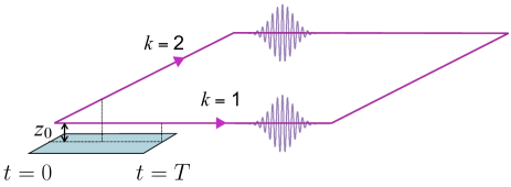
Figure 1: (color online). Atom interferometer interacting with a conducting plate at $z=0$ during the time $T,$ with the arm $k=1$ parallel to the plate (distance $z_{0}$) and the arm $k=2$ flying away with a normal velocity $v_{\perp}.$

The atomic wave-function is initially a coherent superposition $|\psi_{E}(0)\rangle=\frac{1}{\sqrt{2}}\left(|\psi_{E}^{1}(0)\rangle+|\psi_{E}^{2}(0)\rangle\frac{}{}\right)$ of two wave-packets with the same central position but with different initial momenta. These wave-packets will follow two distinct paths $k=1,2$ as illustrated in Fig. 1. The relative phase between these two wave-packets, which determines the local atomic probability function $p(\mathbf{r},t)=|\psi_{E}(\mathbf{r},t)|^{2}$, contains contributions from the atom-surface interaction as well as additional ones independent of the surface.

As in Ref. DoublePath , we extend the atom-optics $ABCD$ formalism Bordé (1991); BordeABCD ; AtomLaserABCD by including the symmetrized DalibardRocCohen interaction energy $U^{\rm int}_{k}(t)$ between the atomic dipole and the EM field within the action phase associated to the external atomic propagation along path $k.$ The atom-surface interaction, assumed weak enough to leave unaltered the shape of the atomic wave-packets during the propagation, results merely in atomic phase shifts.

We evaluate $U^{\rm int}_{k}(t)$ using linear response theory WylieSipe , i.e to lowest order in perturbation theory, and then obtain the local Casimir phase $\varphi^{\rm loc}_{k}=-\frac{1}{\hbar}\int_{0}^{T}dtU_{k}^{\rm int,S}(t)$ along a given path $k$ by picking the surface-dependent contribution $U_{k}^{\rm int,S}(t)$ to the total interaction energy. The key ingredient in our derivation is the introduction of an “on-atom field” operator $\hat{\mathbf{E}}(\hat{\mathbf{r}}_{a}),$ for which the field argument is the atomic position operator $\hat{\mathbf{r}}_{a}$ instead of a classical position $\mathbf{r}_{k}(t)$ taken along the central atomic path $k$.

In the Heisenberg picture, the dipole and the on-atom electric field operators can be expressed as the sum of an unperturbed free-evolving part, defined as $\hat{\mathbf{O}}^{f}(t)=\exp\left(i\hat{H}_{0}t/\hbar\right)\hat{\mathbf{O}}(0)\exp\left(-i\hat{H}_{0}t/\hbar\right)$ with the free Hamiltonian $\hat{H}_{0}=\hat{H}_{E}+\hat{H}_{D}+\hat{H}_{F}$ including the external ($H_{E}$), internal ($H_{D}$) and EM field ($H_{F}$) dofs, and of a contribution $\hat{\mathbf{O}}^{in}(t)$ induced by the atom-field coupling $\hat{H}_{AF}=-\hat{\mathbf{d}}\cdot\hat{\mathbf{E}}(\hat{\mathbf{r}}_{a}).$ To describe the mutual influence between the atomic dipole and the ‘on-atom’ EM field WylieSipe , we introduce temporal correlation functions for the corresponding operators. We also introduce four-point correlation functions for the quantized electric field as discussed below.

Precisely, the dipole and field fluctuations are captured by symmetric correlation functions (also refered to as Hadamard Green’s functions) of the free-evolving operators $\hat{\mathbf{O}}^{f}=\hat{\mathbf{d}}^{f}(t),\hat{\mathbf{E}}(\hat{\mathbf{r}}_{a})^{f}(t),\hat{\mathbf{E}}^{f}(\mathbf{r},t)$ ($\{...\}$ denotes the anti-commutator):

$$G^{H}_{\hat{\mathbf{O}},\>ij}(x;x^{\prime})=\frac{1}{\hbar}\langle\{\hat{O}_{i}^{f}(x),\hat{O}_{j}^{f}(x^{\prime})\}\rangle.$$ (1)

For the dipole and on-atom field operators $\hat{\mathbf{O}}=\hat{\mathbf{d}},\hat{\mathbf{E}}(\hat{\mathbf{r}}_{a})$ the arguments in (1) are two instants $(x;x^{\prime})\equiv(t,t^{\prime})$. For the electric field operator $\hat{\mathbf{O}}=\hat{\mathbf{E}},$ these arguments are two four-vectors $(x;x^{\prime})\equiv(\mathbf{r},t;\mathbf{r}^{\prime},t^{\prime}).$

The linear susceptibilities (polarizability for the dipole), generically written as retarded Green’s functions, describe the linear response of field and dipole to dipole and field perturbations, respectively:

$$G^{R}_{\hat{\mathbf{O}},\>ij}(x;x^{\prime})=\frac{i}{\hbar}\theta(t-t^{\prime})\langle[\hat{O}_{i}^{f}(x),\hat{O}_{j}^{f}(x^{\prime})]\rangle$$ (2)

with $\theta(t-t^{\prime})$ denoting the Heaviside step function.

Note that the on-atom field Green’s functions as defined by (1) and (2) are still quantum operators in the Hilbert space corresponding to the atomic external dofs, since the average is taken over the EM field dofs only. We now take the average $\langle\>\mathcal{G}_{\hat{\mathbf{E}}(\hat{\mathbf{r}}_{a})}^{R,H}(t,t^{\prime})\>\rangle_{k}$ over the external quantum state $|\psi^{k}_{E}\rangle$ corresponding to the single atomic wave-packet $k$. We express the result in terms of the atomic wave-functions $\psi_{E}^{k}(\mathbf{r},t)=\langle\mathbf{r}|e^{-\frac{i}{\hbar}\hat{H}_{E}t}|\psi_{E}^{k}(0)\rangle,$ of the external atomic propagator

$$K(\mathbf{r},t;\mathbf{r}^{\prime},t^{\prime})=\langle\mathbf{r}|e^{-\frac{i}{\hbar}H_{E}(t-t^{\prime})}|\mathbf{r}^{\prime}\rangle,$$ (3)

and of the electric field Green’s functions. For this purpose, we switch to the Schrödinger picture with respect to the external atomic dofs: $\hat{\mathbf{E}}(\hat{\mathbf{r}}_{a})(t)=e^{\frac{i}{\hbar}H_{E}t}\hat{\mathbf{E}}(\hat{\mathbf{r}},t)e^{-\frac{i}{\hbar}H_{E}t}$ with $\hat{\mathbf{r}}=\hat{\mathbf{r}}_{a}(0)$ the atomic position operator, and $\hat{\mathbf{E}}(\mathbf{r},t)$ the quantized electric field (Heisenberg-evolved with respect to the Hamiltonian $H_{F}$) at the classical position $\mathbf{r}$ and time $t$. Using closure relations for the external atomic dofs, one obtains

$$\langle\mathcal{G}_{\hat{\mathbf{E}}(\hat{\mathbf{r}}_{a})}^{R(H)}(t^{\prime},t)\rangle_{k} = \!\iint\!d^{3}\mathbf{r}d^{3}\mathbf{r}^{\prime}\psi_{E}^{k*}(\mathbf{r},t)K(\mathbf{r},t;\mathbf{r}^{\prime},t^{\prime})\psi_{E}^{k}(\mathbf{r}^{\prime},t^{\prime})$$ (4)

$$\qquad\qquad\times\mathcal{G}_{\hat{\mathbf{E}}}^{R(H)}(\mathbf{r},t;\mathbf{r}^{\prime},t^{\prime})\,.$$

It is necessary to identify the physically relevant contributions of the field response (and fluctuations) as far as the atom-surface interaction is concerned. By isotropy of the atomic dipole, only the trace of the electric field Green’s functions $\mathcal{G}^{R(H)}_{\hat{\mathbf{E}}}(x;x^{\prime})\equiv\sum_{i}G^{R(H)}_{\hat{\mathbf{E}}\>ii}(x;x^{\prime})$ (with the sum performed on the Cartesian index $i=1,2,3$) is needed to obtain the interaction energy. $\mathcal{G}^{R(H)}_{\hat{\mathbf{E}}}(x;x^{\prime})$ is the sum of free-space and scattering contributions:

$$\mathcal{G}^{R(H)}_{\hat{\mathbf{E}}}(x;x^{\prime})=\mathcal{G}^{R(H),0}_{\hat{\mathbf{E}}}(x;x^{\prime})+\mathcal{G}^{R(H),S}_{\hat{\mathbf{E}}}(x;x^{\prime})$$ (5)

By symmetry the free-space contributions $\mathcal{G}^{R(H),0}_{\hat{\mathbf{E}}}({\bf r},t;{\bf r}^{\prime},t^{\prime})$ depends only on $|{\bf r}-{\bf r}^{\prime}|$ and $t-t^{\prime}$ Heitler , whereas the scattering contribution $\mathcal{G}^{R(H),S}_{\hat{\mathbf{E}}}({\bf r},t;{\bf r}^{\prime},t^{\prime})$ can be written in terms of the image of the source point ${\bf r}^{\prime}$ in the particular case of a planar perfectly-reflecting surface discussed in Sec. IV. More specifically, the free-space retarded Green’s function $\mathcal{G}^{R,0}_{\hat{\mathbf{E}}}({\bf r},t;{\bf r}^{\prime},t^{\prime})$ represents the direct propagation from ${\bf r}^{\prime}$ to $\bf r$ and does not depend on the distance to the material surface, whereas the scattering contribution $\mathcal{G}^{R,S}_{\hat{\mathbf{E}}}({\bf r},t;{\bf r}^{\prime},t^{\prime})$ corresponds to the propagation with one reflection at the surface.

When replacing (5) into (4), the average on-atom field Green’s functions also split into free-space and scattering contributions, and only the latter contributes to the atom-surface interaction energy $U_{k}^{\rm int,S}(t)$ and hence to the local Casimir phase $\varphi^{\rm loc}_{k}.$ The latter is derived by following steps similar to those employed for point-like wave-packets and using expression (4) with the field Green’s function replaced by the scattering contribution $\mathcal{G}^{R(H),S}_{\hat{\mathbf{E}}}({\bf r},t;{\bf r}^{\prime},t^{\prime}):$

$$\varphi^{\rm loc}_{k}\! = \!\frac{1}{4}\!\iint_{0}^{T}\!dtdt^{\prime}\!\iint\!d^{3}\mathbf{r}d^{3}\mathbf{r}^{\prime}\!\psi_{E}^{k*}(\mathbf{r},t)\!K(\mathbf{r},t;\mathbf{r}^{\prime},t^{\prime})\!\psi_{E}^{k}(\mathbf{r}^{\prime},t^{\prime})$$

$$\times \left[g_{\hat{d}}^{H}(t,t^{\prime})\mathcal{G}_{\hat{\mathbf{E}}}^{R,S}(\mathbf{r},t;\mathbf{r}^{\prime},t^{\prime})+g_{\hat{d}}^{R}(t,t^{\prime})\>\mathcal{G}_{\hat{\mathbf{E}}}^{H,S}(\mathbf{r},t;\mathbf{r}^{\prime},t^{\prime})\right].$$

with $g_{\hat{d}}^{R(H)}(t,t^{\prime})$ representing any diagonal component of the isotropic atomic dipole Green’s function $G^{R(H)}_{\hat{\mathbf{d}},\>ii}(t,t^{\prime}).$ The two contributions appearing in (II) correspond to the separate physical effects responsible for the atom-surface dispersive interaction: radiation reaction and field fluctuations Meschede90 ; Mendes . The former, proportional to the field retarded Green’s function, dominates in the van der Waals un-retarded short-distance limit and is of particular relevance in the following sections. Physically, it represents the self-interaction between the fluctuating dipole at time $t$ and position $\bf r$ with its own electric field, produced at an earlier time $t^{\prime}$ and position ${\bf r}^{\prime},$ after bouncing off the material surface. This interpretation provides an indication that a cross non-local interaction might also exist, with the field produced at one wave-packet component propagating to a different wave-packet component, as discussed in detail in the following sections.

As a first check of (II), we consider the limit of very narrow wave-packets in order to compare with Ref. DoublePath . We assume that the wave-packet width is much shorter than the relevant EM field wave-lengths, and then approximate the position arguments of the Green’s functions $\mathcal{G}_{\hat{\mathbf{E}}}^{(R)H,S}(\mathbf{r},t;\mathbf{r}^{\prime},t^{\prime})$ by the central atomic positions $\mathbf{r}_{k}(t)$ and $\mathbf{r}_{k}(t^{\prime})$ taken along the trajectory $k$ at the respective times $t,t^{\prime}.$ In this case, we can isolate the atomic propagation integral $\psi_{E}^{k}(\mathbf{r},t)=\int d^{3}\mathbf{r}^{\prime}K(\mathbf{r},t;\mathbf{r}^{\prime},t^{\prime})\!\psi_{E}^{k}(\mathbf{r}^{\prime},t^{\prime})$ in (II) and find

$$\varphi^{\rm loc}_{k}\! \approx \!\frac{1}{4}\!\iint_{0}^{T}\!dtdt^{\prime}\!\left[\frac{}{}g_{\hat{d}}^{H}(t,t^{\prime})\mathcal{G}_{\hat{\mathbf{E}}}^{R,S}(r_{k}(t),r_{k}(t^{\prime}))\right.$$

$$\left.\qquad\qquad\qquad\qquad+g_{\hat{d}}^{R}(t,t^{\prime})\>\mathcal{G}_{\hat{\mathbf{E}}}^{H,S}(r_{k}(t),r_{k}(t^{\prime}))\frac{}{}\right].$$

in agreement with Ref. DoublePath .

A second, more important limiting case of Eq. (II), corresponds to its quasi-static limit. We also assume thermal equilibrium for the dipole and EM field dofs, and consider long interaction times (stationary regime). In this case, the dipole and electric field Green’s functions depend only on the time difference $\tau=t-t^{\prime}$ and not on the individual times. The retarded Green’s functions $\mathcal{G}_{\hat{\mathbf{E}}}^{R,S}(\mathbf{r},\tau;\mathbf{r}^{\prime},0)$ is non-zero only for a time delay $\tau$ equal to the time it takes for a photon to travel from the source position $\mathbf{r}^{\prime}$ to the position $\mathbf{r}$ after one reflection at the surface. These durations are, in usual experimental conditions, much shorter than the time scales associated with the external atomic motion. In the quasi-static limit, we treat the external atomic motion as completely “frozen” during the time delay $\tau=t-t^{\prime}$. In other words, we take $t^{\prime}:=t$ in the external atomic propagator and wave-functions. In this limit, the former simplifies to $K(\mathbf{r},t;\mathbf{r}^{\prime},t)=\delta(\mathbf{r}-\mathbf{r}^{\prime})$. The resulting expression can be directly compared with the formula for the dispersive atom-surface potential $V_{\rm Cas}({\bf r})$ WylieSipe as detailed in the Appendix. We then find that the local phase becomes a time integral of the dispersive potential taken at the instantaneous atomic position weighted by the external probability density:

$$\varphi^{\rm loc}_{k}\approx-\frac{1}{\hbar}\int_{0}^{T}dt\int d^{3}\mathbf{r}\>|\psi_{E}^{k}(\mathbf{r},t)|^{2}\>V_{\rm{Cas}}(\mathbf{r}).$$ (8)

The quasi-static expression (8) was employed as the theoretical model for comparison with experiments Cronin04 ; CroninVigue ; Lepoutre11 . On the other hand, our more general result (II) allows for non-equilibrium Ryan11 ; Antezza and non-stationary regimes which cannot be described by the more standard expression (8). Explicit results for the dynamical corrections to order ${\bf\dot{r}}_{k}(t)/c$ were derived in Ref. NonAdditiveCasimir in the case of very narrow atomic packets flying close to a perfectly-reflecting planar surface. Note, however, that we also find non-local atomic phase corrections to order ${\bf\dot{r}}_{k}(t)/c.$ Thus, a full quantum open system approach, to be developed in the next sections, is required to assess the first-order dynamical correction in a consistent way.

III NON-LOCAL DYNAMICAL CASIMIR ATOMIC PHASES

From now on, we no longer model the effect of surface interactions as a local phase shift imprinted on each external atomic wave-packet. We consider instead the evolution of the full quantum state describing the external atomic waves, atomic dipole and EM field. In the discussion to follow, we will refer respectively to the dipole and EM field dofs as the “environment” and to the external atomic waves as the “system”. We consider the case of point-like wave-packets in this section, so as to introduce our method in a simpler setting, thus paving the way for the discussion of finite-width wave-packets in the following sections.

We describe here how the quantum state of the environment is affected by the propagation of the external atomic waves. Because it involves the center-of-mass position operator $\hat{\mathbf{r}}_{a}$, the dipolar Hamiltonian $\hat{H}_{AF}=-\hat{\mathbf{d}}\cdot\hat{\mathbf{E}}(\hat{\mathbf{r}}_{a})$ operates on the environment in a manner which depends on the path followed by the atoms. Thus, such a Hamiltonian acts as a “which-path” marker, leaving an atomic “footprint” on the dipole and EM field quantum states. The phase contribution is of second order in the dipolar interaction Hamiltonian. A Feynman-diagram expansion shows that these footprints actually contain cross terms, involving the two coherent components of the external atomic state propagating on two distinct arms of the interferometer (see Fig. 2). As discussed in detail below, such terms reflect a non-local disturbance of the environment operated at different times by the system. In addition to a loss of contrast in the fringe pattern, such perturbation also induces a non-local double-path atomic phase coherence. We derive here both the local and non-local phases resulting from the influence of the environment. The local phase shifts obtained below correspond exactly to the atom-surface interaction phases  (II) and (II) derived in the previous section for finite-width and point-like wave-packets, respectively, whereas the non-local phases cannot be derived from the interaction energy along the different paths taken separately.

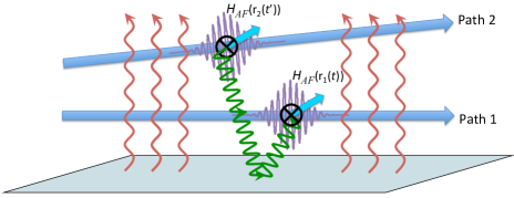
Figure 2: (color online). Double-path footprint left on the environment (dipole + EM field) by the external atomic state through the dipolar interaction $\hat{H}_{AF}.$

In Ref. DoublePath , we have briefly outlined an alternative approach, based on the influence functional, which captures the effect of the environment on very narrow atomic waves as a complex phase which can also be recast as a stochastic phase Ryan11 . This method leads to the same final results we derive in this section. The equivalence between the two points of views illustrates an important property of open systems SAI90 : its evolution is equally well described by considering the accumulation of a stochastic phase, or by analyzing the trace left by the system onto the quantum state of the environment.

III.1 Atomic interferences in presence of an environment

Inspired by Ref. SAI90 , we calculate the time evolution of the full quantum state, which is initially given by $|\psi(0)\rangle=\frac{1}{\sqrt{2}}\left(|\psi_{E}^{1}(0)\rangle+|\psi_{E}^{2}(0)\rangle\right)\otimes|\Psi_{DF}(0)\rangle,$ where $|\Psi_{DF}(0)\rangle=|\psi_{D}(0)\rangle\!\otimes\!|\psi_{F}(0)\rangle$ denotes the initial environment (internal dipole and EM field) quantum state. We discard the influence of the atom-surface interaction on the external atomic motion (prescribed atomic trajectories), which is a very good approximation in usual experimental conditions CroninVigue . In this section, we assume, for simplicity, that the wave-packet width is much smaller than the relevant field wavelengths (more general results are derived in the following sections). Thus, the interaction is described by the Hamiltonians $\hat{H}_{AF}(\mathbf{r}_{k}(t))=-\hat{\mathbf{d}}\cdot\hat{\mathbf{E}}(\mathbf{r}_{k}(t))$ parametrized by the wave-packet trajectories represented by the four-vectors $r_{k}(t)\equiv(\mathbf{r}_{k}(t),t)$ with $k=1,2$, and acting only on the dipole and EM field Hilbert spaces foot_Rontgen . We work in the interaction picture and the transformed time-dependent interaction Hamiltonian reads

$$\hat{\widetilde{H}}_{AF}(r_{k}(t))=e^{\frac{i}{\hbar}(\hat{H}_{D}+\hat{H}_{F})t}\left(-\hat{\mathbf{d}}\cdot\hat{\mathbf{E}}(\mathbf{r}_{k}(t))\right)e^{-\frac{i}{\hbar}(\hat{H}_{D}+\hat{H}_{F})t}.$$ (9)

At time $t=T$, the full quantum state reads

$$|\psi(T)\rangle = \frac{1}{\sqrt{2}}|\psi_{E}^{1}(T)\rangle\!\otimes\!\mathcal{T}e^{-\frac{i}{\hbar}\int_{0}^{T}dt\hat{\widetilde{H}}_{AF}(r_{1}(t))}|\Psi_{DF}(0)\rangle$$

$$+ \frac{1}{\sqrt{2}}|\psi_{E}^{2}(T)\rangle\!\otimes\!\mathcal{T}e^{-\frac{i}{\hbar}\int_{0}^{T}dt^{\prime}\hat{\widetilde{H}}_{AF}(r_{2}(t))}\!|\Psi_{DF}(0)\rangle,$$

where $\mathcal{T}$ denotes the time-ordering operator.

Since the dipole and EM field states are not measured in the experiment, we calculate the external reduced density operator $\rho={\rm Tr}_{DF}\left(|\psi(T)\rangle\langle\psi(T)|\right).$ When replacing (LABEL:psi) into this equation, the cross (interference) term represents the external atomic coherence, which we evaluate in the position representation:

$$\rho_{12}({\bf r},{\bf r}^{\prime};T)=\frac{1}{2}\,\langle{\bf r}|\psi_{E}^{1}(T)\rangle\langle\Psi_{DF}^{2}(T)|\Psi_{DF}^{1}(T)\rangle\langle\psi_{E}^{2}(T)|{\bf r}^{\prime}\rangle$$ (11)

Thus, the interference term $\rho_{12}^{(0)}=\frac{1}{2}\psi_{E}^{2}(\mathbf{r}^{\prime},T)^{*}\,\psi_{E}^{1}(\mathbf{r},T)$ is now multiplied by the scalar product of the disturbed environment states

$$\langle\Psi_{DF}^{2}(T)|\Psi_{DF}^{1}(T)\rangle \equiv e^{i\Phi_{12}}.$$ (12)

The complex phase $\Phi_{12}$ captures the environment effect on the external interference term accumulated over the interaction time $T$:

$$e^{i\Phi_{12}} = \langle\Psi_{DF}(0)|\widetilde{\mathcal{T}}e^{\frac{i}{\hbar}\int_{0}^{T}dt\hat{\widetilde{H}}_{AF}(r_{2}(t))}$$ (13)

$$\times\mathcal{T}e^{-\frac{i}{\hbar}\int_{0}^{T}dt\hat{\widetilde{H}}_{AF}(r_{1}(t))}\!|\Psi_{DF}(0)\rangle$$

with $\widetilde{\mathcal{T}}$ denoting the anti-time-ordering operator (earlier-time operators on the left).

In general the final environmental quantum states have a scalar product smaller than unity $|\langle\Psi^{2}_{DF}(T)|\Psi^{1}_{DF}(T)\rangle|=e^{-{\rm Im}\Phi^{E}_{12}}<1,$ leading to an attenuation of the interferometer fringe pattern. In this case, the full quantum state $|\psi(T)\rangle$ given by (LABEL:psi) is entangled, indicating the transfer of which-path information on the atomic motion to the environment. The resulting decoherence has been theoretically studied CasimirDecoherence and measured Sonnentag07 for charged particles close to a material surface. Here we focus on the complementary effect that is also present in the general formula (13) for the complex phase $\Phi_{12}.$ In addition to the loss of fringe visibility, the coupling with the dipole and EM field dofs also leads to a displacement of the interference fringes, corresponding to the real part ${\rm Re}\,\Phi_{12},$ which we analyze in more detail in the remaining part of this paper.

III.2 Diagrammatic expansion of the environment-induced phase

As in the previous section, we follow a linear response approach and treat the dipolar coupling as a small perturbation. Thus, we perform a diagrammatic expansion of the time-ordered (and anti-time-ordered) exponentials appearing in the the formula (13) for the environment-induced complex phase $\Phi_{12}$ . We focus on the lowest-order diagrams yielding a finite phase. Special care is required, since the dipolar coupling Hamiltonians $\hat{\widetilde{H}}_{AF}(r_{k}(t))$ (9) taken at different times do not commute. We calculate $\Phi_{12}$ to first order in the atomic polarizability, allowing us to approximate $e^{i\Phi_{12}}\simeq 1+i\Phi_{12}.$ This is a valid approximation as long as the distance between the atom and the plate is much larger than the atomic size (this assumption also justifies the electric dipole approximation).

It follows from (13) that first-order diagrams are proportional to ($\langle...\rangle_{0}$ denoting the average over the intial environment state $|\Psi_{DF}(0)\rangle$)

$$\pm\frac{i}{\hbar}\int_{0}^{T}dt\,\langle\,\hat{\mathbf{d}}(t)\cdot\hat{\mathbf{E}}({\bf r}_{k}(t))\,\rangle_{0}.$$ (14)

and as a consequence vanish since the the atom has no permanent dipole moment.

Thus, we focus on second-order diagrams, which are quadratic in the EM field and dipole operators. There are two different ways to build second-order diagrams from Eq. (13): one can either take two interactions pertaining to the same time-ordered (or anti-time-ordered) exponential, or one may take one interaction from each exponential. Diagrams of the first kind correspond to a sequence of interactions along the same path, and are referred to as “single-path” (SP) diagrams. Diagrams of the second kind involve simultaneously two distinct paths, and are thus called “double-path” (DP) diagrams. The two contributions sum up to give the complex environment-induced phase $\Phi_{12}=\Phi^{\rm SP}_{12}+\Phi^{\rm DP}_{12}$.

III.2.1 Phase contribution of local single-path diagrams

We consider first the two possible SP diagrams, beginning with the diagram arising from the time-ordered exponential evaluated along the path $1$ in the r.-h.-s. of (13), whose contribution reads:

$$\Phi^{\rm{SP}}_{1}=\!\frac{i}{\hbar^{2}}\!\int_{0}^{T}dt\!\int_{0}^{t}dt^{\prime}\!\sum_{i,j}\langle\>\hat{d}_{i}(t)\hat{d}_{j}(t^{\prime})\hat{E}_{i}(r_{1}(t))\hat{E}_{j}(r_{1}(t^{\prime}))\>\rangle_{0}$$ (15)

where we sum over the Cartesian indices $i,j=1,2,3$. In order to express the phase $\Phi^{\rm{SP}}_{1}$ in terms of dipole and electric field Green’s functions (1,2), we write the product of dipole (or electric field) operators at distinct times (or space-time points) as the half sum of their commutator and anti-commutator. As in Sec. II, these contributions can be expressed in terms of the scalar dipole $g^{R(H)}_{\hat{d}}(t,t^{\prime})$ and the trace of the electric field Green’s function $\mathcal{G}^{R(H)}_{\hat{\bf E}}(x;x^{\prime}).$ For the latter we take only the scattering contribution $\mathcal{G}^{R(H),S}_{\hat{\bf E}}(x;x^{\prime})$ [see Eq. (5)] and then find that ${\rm Re}\,\Phi^{\rm{SP}}_{1}=\varphi^{\rm loc}_{1}$ is precisely the local phase (II) obtained in Sec. II for point-like wave-packets.

An analogous SP diagram comes from the anti-time ordered exponential along path $2$ in the r.-h.-s. of (13), yielding a similar contribution $\Phi^{\rm{SP}}_{2}$ to the complex phase. The reversed time-ordering leads to an additional minus sign in front of each retarded dipole and electric field Green’s functions appearing in the expression for the complex phase. Since ${\rm Re}\,\Phi^{\rm{SP}}_{2}$ contains an odd number of retarded Green’s functions, we find ${\rm Re}\,\Phi^{\rm{SP}}_{2}=-\varphi^{\rm loc}_{2}$ with the local phase $\varphi^{\rm loc}_{2}$ given again by  (II). Thus, the total contribution of single-path diagrams has a real part

$${\rm Re}\,\Phi_{12}^{\rm SP}=\varphi^{\rm loc}_{1}-\varphi^{\rm loc}_{2}$$ (16)

Since ${\rm Re}\,\Phi_{12}$ represents the phase coherence of path 1 with respect to path 2, it must be anti-symmetric with respect to the interchange of the two paths. This property is clearly satisfied by the local contribution (16), and will also hold for the non-local double-path contribution discussed in the following. On the other hand, the imaginary part ${\rm Im}\,\Phi_{12},$ representing decoherence, must be symmetric with respect to the interchange, with both local path contributions being positive and thus leading to an attenuation of fringe pattern. This property is also satisfied by the result derived from (13) since ${\rm Im}\,\Phi_{12}$ contains an even number of retarded Green’s functions.

In short, the local approach developed in Section II provides the correct expressions for the real part of the single-path contributions to the complex phase $\Phi_{12}.$ However, it is unable to yield even the single-path contributions to the imaginary part of $\Phi_{12},$ which represents the decoherence effect. More importantly, the local theory also misses all double-path phase contributions, which we discuss in the remaining part of this section.

III.2.2 Phase contribution of the non-local double-path diagram

We investigate here the double-path diagram, which involve a product of linear terms issued from both the time-ordered and anti-time-ordered exponentials in the r.-h.-s. of (13):

$$i\Phi^{\rm{DP}}_{12} = \!\Biggl{\langle}\>\sum_{i,j}\left(\frac{i}{\hbar}\!\int_{0}^{T}dt^{\prime}\hat{d}_{i}(t^{\prime})\hat{E}_{i}(r_{2}(t^{\prime}))\right)$$ (17)

$$\times\left(\frac{-i}{\hbar}\int_{0}^{T}dt\hat{d}_{j}(t)\hat{E}_{j}(r_{1}(t))\right)\>\>\Biggr{\rangle}_{0}$$

As previously, we express the product of two dipole and EM field operators as the half sum of their commutators and anti-commutators. After summing over the Cartesian indices $i,j$ and discarding the contributions from the free-space electric field Green’s functions, we find for the real part $\phi^{\rm{DP}}_{12}\equiv{\rm Re}\,\Phi^{\rm{DP}}_{12}$

$$\phi^{\rm{DP}}_{12}\! \!=\! \!\frac{1}{4}\!\!\iint_{0}^{T}\!dt^{\prime}dt\left[\frac{}{}g_{\hat{d}}^{H}(t,t^{\prime})\left(\mathcal{G}_{\hat{\mathbf{E}}}^{R,S}(r_{1}(t),r_{2}(t^{\prime}))-\mathcal{G}_{\hat{\mathbf{E}}}^{R,S}(r_{2}(t),r_{1}(t^{\prime}))\right)+g_{\hat{d}}^{R}(t,t^{\prime})\left(\mathcal{G}_{\hat{\mathbf{E}}}^{H,S}(r_{1}(t),r_{2}(t^{\prime}))-\mathcal{G}_{\hat{\mathbf{E}}}^{H,S}(r_{2}(t),r_{1}(t^{\prime}))\right)\right]$$

As required for consistency, the r.-h.-s. of (LABEL:eq:double_path_phase) is anti-symmetrical under the interchange of the two paths, since $\phi^{\rm{DP}}_{12}$ represents a contribution to the relative phase of path 1 with respect to path 2. Remarkably, this relative phase contribution depends simultaneously on the two distinct paths of the atom interferometer and cannot be split into separate contributions from paths 1 and 2.

The non-negligible contribution to the non-local phase $\phi^{\rm{DP}}_{12}$ actually comes entirely from the term proportional to $g_{\hat{d}}^{H}(t,t^{\prime})$ in Eq. (LABEL:eq:double_path_phase), which accounts for the long-lived atomic dipole fluctuations. Eq. (LABEL:eq:double_path_phase) shows that the non-local phase results from the asymmetry between the cross self-interactions involving different wave-packets — the fluctuating dipole interacting with the electric field sourced by itself at a different location DoublePath .

IV DYNAMICAL CASIMIR PHASES FOR FINITE-SIZE WAVE-PACKETS

The previous derivation of the dynamical Casimir phases for point-like atomic wave-packets highlighted the basic physical mechanisms behind the appearance of a non-local double-path Casimir phase. However, usual experimental conditions in Casimir interferometry Cronin04 ; CroninVigue ; Lepoutre11 do not match this assumption, since the width of the atomic wave-packets are of the same order of the atom-surface distances. In this section, we present a derivation of the dynamical local and non local Casimir phases for finite-width wave-packets.

As in the previous section, we consider the interaction picture. However, we no longer consider the interaction Hamiltonian as parametrized by well-defined atomic trajectories. Instead, we now evolve the interaction Hamiltonian with respect to the external atomic dofs associated to the Hamiltonian $\hat{H}_{E}$, i.e. the time-dependent interaction Hamiltonian can be expressed as a function of the free-evolving dipole $\hat{\mathbf{d}}(t)$, free-evolving electric field $\hat{\mathbf{E}}(\mathbf{r},t)$ and initial time position operator $\hat{\mathbf{r}}_{a}$ as $\hat{\widetilde{H}}_{AF}(t)=e^{\frac{i}{\hbar}\hat{H}_{E}t}\left[-\hat{\mathbf{d}}(t)\cdot\hat{\mathbf{E}}(\hat{\mathbf{r}}_{a},t)\right]e^{-\frac{i}{\hbar}\hat{H}_{E}t}$. Again, we consider the coherence of the reduced density matrix (11) $\rho_{12}(\mathbf{r},\mathbf{r}^{\prime},t)$ between the two wave-packets $\psi_{E}^{1}(\mathbf{r},t)$ and $\psi_{E}^{2}(\mathbf{r}^{\prime},t)$, related to the free-evolving density matrix coherence $\rho^{0}_{12}(\mathbf{r},\mathbf{r}^{\prime};T)=\frac{1}{2}\psi_{E}^{1}(\mathbf{r},t)\psi_{E}^{2*}(\mathbf{r}^{\prime},t)$ by $\rho_{12}(\mathbf{r},\mathbf{r}^{\prime};T)=\rho^{0}_{12}(\mathbf{r},\mathbf{r}^{\prime};T)e^{i\phi_{12}(\mathbf{r},\mathbf{r}^{\prime},T)}$. For a small interaction phase $\phi_{12}(\mathbf{r},\mathbf{r}^{\prime};T)$, a first-order Taylor expansion yields $\phi_{12}(\mathbf{r},\mathbf{r}^{\prime};T)\simeq(-i)\delta\rho_{12}(\mathbf{r},\mathbf{r}^{\prime};T)/\rho^{0}_{12}(\mathbf{r},\mathbf{r}^{\prime};t)$. We have introduced the difference between the free and interacting density matrix coherences $\delta\rho_{12}(\mathbf{r},\mathbf{r}^{\prime};T)=\rho_{12}(\mathbf{r},\mathbf{r}^{\prime};T)-\rho^{0}_{12}(\mathbf{r},\mathbf{r}^{\prime};T)$, determined below in terms of second-order dipolar interaction diagrams. We also define the average interaction phase coherence $\phi_{12}(T)\equiv\iint d^{3}\mathbf{r}d^{3}\mathbf{r}^{\prime}|\psi_{E}^{1}(\mathbf{r},T)|^{2}|\psi_{E}^{2}(\mathbf{r}^{\prime},T)|^{2}\phi_{12}(\mathbf{r},\mathbf{r}^{\prime};T)$, equivalently expressed as

$$\phi_{12}(T)=-2i\int d^{3}\mathbf{r}\int d^{3}\mathbf{r}^{\prime}\psi_{E}^{1*}(\mathbf{r},T)\psi_{E}^{2}(\mathbf{r}^{\prime},T)\;\delta\rho_{12}(\mathbf{r},\mathbf{r}^{\prime};T).$$ (19)

At the time $T$, the reduced density matrix can be formally expressed as

$$\rho_{12}(\mathbf{r},\mathbf{r}^{\prime};T) = \frac{1}{2}\langle\psi_{DF}(0)|\otimes\langle\psi_{E}^{2}(0)|\widetilde{\mathcal{T}}\left[e^{\frac{i}{\hbar}\int_{0}^{T}dt\hat{\widetilde{H}}_{AF}(t)}\right]$$

$$\times\left(e^{\frac{i}{\hbar}H_{E}T}|\mathbf{r}^{\prime}\rangle\langle\mathbf{r}|e^{-\frac{i}{\hbar}H_{E}T}\otimes{\bf 1}_{DF}\right)$$

$$\times\mathcal{T}\left[e^{-\frac{i}{\hbar}\int_{0}^{T}dt^{\prime}\hat{\widetilde{H}}_{AF}(t^{\prime})}\right]|\psi_{E}^{1}(0)\rangle\otimes|\psi_{DF}(0)\rangle$$

Let us first investigate the SP paths terms, which correspond to contributions to $\delta\rho_{12}(\mathbf{r},\mathbf{r}^{\prime},T)$ arising from quadratic terms issued from the same time-ordered (or anti-time ordered) exponential. One considers without loss of generality the SP phase associated with path $1$, which yields the contribution:

$$\delta\rho_{12}^{\rm SP1}(\mathbf{r}_{1},\mathbf{r}_{2};T)=\frac{i}{2\hbar^{2}}\psi_{E}^{2*}(\mathbf{r}_{2},T)\sum_{i,j=1}^{3}\int_{0}^{T}dt\int_{0}^{t}dt^{\prime}$$

$$\times \int d^{3}\mathbf{r}\int d^{3}\mathbf{r}^{\prime}K(\mathbf{r}_{1},T;\mathbf{r},t)K(\mathbf{r},t;\mathbf{r}^{\prime},t^{\prime})\psi_{E}^{1}(\hat{\mathbf{r}}^{\prime},t^{\prime})$$

$$\times \langle\widetilde{\psi}_{DF}(0)|\hat{d}_{i}(t)\hat{E}_{i}(\mathbf{r},t)\hat{d}_{j}(t^{\prime})\hat{E}_{j}(\mathbf{r}^{\prime},t^{\prime})|\widetilde{\psi}_{DF}(0)\rangle$$

When taking the average (19) of $\delta\rho_{12}^{\rm SP1}$, one recognizes an integral involving the external atomic propagator (3), leading to the Casimir phase (II) obtained previously with the local theory.

On the other hand, one derives the DP phase from Eq. (IV) by considering the diagrams composed of linear terms issued from both the time-ordered and anti-time ordered exponentials:

$$\delta\rho_{12}^{\rm DP}(\mathbf{r},\mathbf{r}^{\prime};T)=\frac{1}{2}\sum_{i,j=1}^{3}\int d^{3}\mathbf{r}\int d^{3}\mathbf{r}^{\prime}\langle\psi_{DF}(0)|$$

$$\left[\frac{i}{\hbar}\int_{0}^{T}dt^{\prime}\psi_{E}^{2*}(\mathbf{r}^{\prime},t^{\prime})K(\mathbf{r}^{\prime},t^{\prime};\mathbf{r}_{2},T)\hat{d}_{i}(t^{\prime})\hat{E}_{i}(\mathbf{r}^{\prime},t^{\prime})\right]$$

$$\left[-\frac{i}{\hbar}\int_{0}^{T}dt\hat{d}_{j}(t)\hat{E}_{j}(\mathbf{r},t)K(\mathbf{r}_{1},T;\mathbf{r},t)\psi_{E}^{1}(\mathbf{r},t)\right]|\psi_{DF}(0)\rangle.$$

The averaging procedure (19) yields a double-path phase which depends simultaneously on the histories of the two wave-functions corresponding to each interferometer arm. As in Section III, we express the bilinear averages of the dipole and field operators in terms of Hadamard and retarded Green’s functions:

$$\phi^{\rm{DP}}_{12}(T) = \frac{1}{4}\iint_{0}^{T}dtdt^{\prime}\iint d^{3}\mathbf{r}d^{3}\mathbf{r}^{\prime}\left|\psi_{E}^{1}(\mathbf{r},t)\right|^{2}|\psi_{E}^{2}(\mathbf{r}^{\prime},t^{\prime})|^{2}$$

$$\times \left[\frac{}{}g_{\hat{d}}^{H}(t,t^{\prime})\left(\mathcal{G}_{\hat{\mathbf{E}}}^{R,S}(\mathbf{r},t;\mathbf{r}^{\prime},t^{\prime})-\mathcal{G}_{\hat{\mathbf{E}}}^{R,S}(\mathbf{r}^{\prime},t^{\prime};\mathbf{r},t)\right)\right.$$

$$+ \left.g_{\hat{d}}^{R}(t,t^{\prime})\left(\mathcal{G}_{\hat{\mathbf{E}}}^{H,S}(\mathbf{r},t;\mathbf{r}^{\prime},t^{\prime})-\mathcal{G}_{\hat{\mathbf{E}}}^{H,S}(\mathbf{r}^{\prime},t;\mathbf{r},t^{\prime})\right)\frac{}{}\right]$$

If one considers that the electric field Green’s functions are uniform over the width of atomic wave-packets, one obviously retrieves the nonlocal DP phase (LABEL:eq:double_path_phase) of Section III obtained in the narrow atomic wave-packet limit. In order to highlight the dependence of the DP phase on the dynamical atomic motion, we Taylor expand the advanced time wave-function $|\psi_{E}^{k}(\mathbf{r},t)|^{2}\simeq|\psi_{E}^{k}(\mathbf{r},t^{\prime})|^{2}+\frac{\partial}{\partial t}|\psi_{E}^{k}(\mathbf{r},t^{\prime})|^{2}\tau$ in Eq. (IV). This is an excellent approximation since the time $\tau=|{\bf r}-{\bf r}^{\prime}|/c$ corresponds to the light propagation between the dipole and its image, and is thus extremely short compared to the typical time scale of the external atomic motion. As before, we assume a stationary regime and write $g^{R,H}_{\hat{d}}(\tau)\equiv g^{R,H}_{\hat{d}}(t^{\prime}+\tau,t^{\prime})$. Using the conservation of the atomic probability, one can express the DP phase (IV) in terms of the probability current $\mathbf{j}^{k}(\mathbf{r},t)=\mbox{Re}\left[\psi_{E}^{k*}(\mathbf{r},t)\frac{\hbar}{im}\nabla\psi_{E}^{k}(\mathbf{r},t)\right]$:

$$\phi^{\rm{DP}}_{12}(T)=\frac{1}{4}\sum_{i=1}^{3}\int_{0}^{T}dt^{\prime}\int_{0}^{T-t^{\prime}}d\tau\iint d^{3}\mathbf{r}d^{3}\mathbf{r}^{\prime}$$ (22)

$$\times \left(\frac{}{}j_{i}^{1}(\mathbf{r},t^{\prime})|\psi_{E}^{2}(\mathbf{r}^{\prime},t^{\prime})|^{2}-j_{i}^{2}(\mathbf{r},t^{\prime})|\psi_{E}^{1}(\mathbf{r}^{\prime},t^{\prime})|^{2}\frac{}{}\right)\>\tau$$

$$\times \left(\frac{}{}g_{\hat{d}}^{H}(\tau)\frac{\partial\mathcal{G}_{\hat{\mathbf{E}}}^{R,S}(\mathbf{r},t^{\prime}+\tau;\mathbf{r}^{\prime},t^{\prime})}{\partial r_{i}}\right.$$

$$\left.\frac{}{}+g_{\hat{d}}^{R}(\tau)\frac{\partial\mathcal{G}_{\hat{\mathbf{E}}}^{H,S}(\mathbf{r},t^{\prime}+\tau;\mathbf{r}^{\prime},t^{\prime})}{\partial r_{i}}\right).$$

The non-local DP phase is thus a dynamical phase correction, with the current density giving the probability density evolution during the very short electromagnetic propagation time $\tau.$ In the next section, we investigate in greater detail the phases acquired by wide wave-packets flying close to a planar perfectly-reflecting surface.

V NON-LOCAL DYNAMICAL CORRECTIONS TO THE VAN DER WAALS PHASE FOR A PLANE SURFACE

In this section, we derive explicit results for the non-local dynamical contributions to the Casimir phase, working at the leading order in $v/c$ ($v$ denotes the magnitude of the atomic center-of-mass velocity). Starting from the general results of Sec. IV, we describe such corrections for wide atomic packets interacting with a perfectly-reflecting planar surface, located at $z=0.$ Moreover, we shall consider specifically the short-distance van der Waals (vdW) regime probed by the experiments Cronin04 ; CroninVigue ; Lepoutre11 , which corresponds to a stronger atom-surface interaction (thus yielding larger dynamical phase corrections) than the long-distance Casimir-Polder limit. As discussed in Section II, at these distances the dominant dynamical vdW phase contributions come from the electric field response to dipole fluctuations. The experiments were performed for wide atomic wave-packets filling in the gap between the central trajectory and the conducting plate Cronin04 ; CroninVigue ; Lepoutre11 . In this case, we show here that the non-local DP phase is enhanced with respect to the result for point-like packets DoublePath by a logarithmic factor.

We take a Mach-Zehnder atom interferometer in the half-space $z>0$ close to the material surface at $z=0$ as illustrated by Fig. 1. The two central atomic trajectories share the same velocity component parallel to the plate, but have arbitrary normal velocities:

$$\mathbf{r}_{k}(t)=\mathbf{r}_{0/\!\!/}(t)+z_{k}(t)\,\hat{\mathbf{z}},\quad k=1,2.$$ (23)

The results to follow can be extended to discuss dynamical vdW phase corrections resulting from atomic interactions with a grating as in Refs. Cronin04 ; CroninVigue ; Lepoutre11 .

V.1 Electric field and dipole Green’s functions

It is necessary, at this stage, to have at hand explicit expressions for the dipole and electric field Green’s functions. As discussed in Section II, the electric field Green’s functions is decomposed as the sum of free and scattering contributions. Only the latter is relevant for the derivation of the Casimir phases induced by the surface. We first derive the field Green’s functions in Fourier space by writing the electric field operator as a sum over normal modes, taking due account of the perfectly-reflecting surface at $z=0.$ We then derive both the known result for the free-space Green’s function Heitler as well as the scattering contribution

$$\mathcal{G}_{\hat{\mathbf{E}}}^{R,S}(x,x^{\prime}) = \frac{\theta(\tau)}{2\pi\epsilon_{0}}\frac{\partial^{2}}{\partial z\partial z^{\prime}}\left(\frac{\delta(\tau-|\mathbf{r}-\mathbf{r}^{\prime}_{\rm I}|/c)}{|\mathbf{r}-\mathbf{r}^{\prime}_{\rm I}|}\right)$$ (24)

As expected $\mathcal{G}_{\hat{\mathbf{E}}}^{R,S}(x,x^{\prime})$ depends on the time difference $\tau=t-t^{\prime}$ only and not on the individual times. It is written in terms of the propagation distance $|\mathbf{r}-\mathbf{r}^{\prime}_{\rm I}|$ between the point $\bf{r}$ and the image $\mathbf{r}^{\prime}_{\rm I}=(x^{\prime},y^{\prime},-z^{\prime})$ of the source point ${\bf r}^{\prime}=(x^{\prime},y^{\prime},z^{\prime})$ with respect to the plane surface. Assuming the EM field to be in thermal equilibrium, the electric field Hadamard Green’s function $\mathcal{G}_{\hat{\mathbf{E}}}^{H,S}(x,x^{\prime})$ can be obtained from the retarded one thanks to the fluctuation-dissipation theorem.

In order to obtain the dipole Green’s functions, we model the internal atomic degrees of freedom as an harmonic oscillator with a transition frequency $\omega_{0}$ (and wave-length $\lambda_{0}$) and assume the atom to be in its ground state. The Hadamard dipole Green’s function is then proportional to the static atomic polarizability $\alpha(0):$

$$g^{H}_{\hat{d}}(t,t^{\prime})=\alpha(0)\,\omega_{0}\,\cos[\omega_{0}(t-t^{\prime})].$$ (25)

V.2 Nonlocal dynamical phases

We consider the limit of wide atomic packets with a well-defined momentum, which is well-suited to describe the dispersion effects associated to the finite width of the atomic packets propagating nearby the plate. In this limit, one may take the probability current involved in the DP path phase (22) as $\mathbf{j}^{k}(\mathbf{r},t)\simeq|\psi_{E}^{k}(\mathbf{r},t)|^{2}\mathbf{v}_{k}(t)$ where $\mathbf{v}_{k}(t)={\bf\dot{r}}_{k}(t)$ is a classical velocity RemarkWidePacketApprox . Since the DP phase depends sharply on the distance between the atoms and the conductor and not on their lateral position above this surface, the extension of the atomic wave-packets in the direction $O_{z}$ normal to the conducting surface is much more critical than the extension of the atomic packets along the directions $O_{x},O_{y}$ parallel to the conductor. Thus, one can safely use one-dimensional atomic wave-packets $\psi_{E}^{1,2}(z,t)$ in order to model dispersion effects in the nonlocal DP phase acquired by wide atomic beams.

We first model the atomic wave-functions by a step-wise distribution centered on the classical atomic trajectories of time-independent width, i.e. we take $|\psi_{k}^{E}(z,t)|^{2}=1/w$ for $z_{k}(t)-w/2<z<z_{k}(t)+w/2$ and zero for $|z-z_{k}(t)|\geq w/2$ – with a width $w$ such that $w\leq 2z_{0}$ where $z_{0}=z_{1}(0)=z_{2}(0)$ is the initial distance between the atomic wave-packet centers and the plate. Naturally, such description is a simple approximation, and a modelling in terms of Gaussian wave-packets would be more accurate. Nevertheless, this approach should yield the correct qualitative picture and has the advantage of giving analytical expressions regarding the dependence of the DP phase towards the wave-packet width.

We calculate the DP phase in the short-distances vdW regime and take $g_{d}^{H}(\tau)\approx g_{d}^{H}(0)=\omega_{0}\alpha(0)$ [see (25)]. We consider the linear trajetories (23), and assume that the distance between the central trajectory endpoints is much larger than the initial altitude $z_{0}$, yielding the saturation limit of the DP phase DoublePath . Using the step wave-functions in Eq.(22), one obtains an expression for the DP phase taking into account the finite atomic packet extension:

$$\phi^{\rm DP}_{12}(z_{0},w)=-\frac{3\pi}{\lambda_{0}}\frac{\alpha(0)}{4\pi\epsilon_{0}}\frac{1}{w^{2}}\log\left(1-\frac{w^{2}}{4z_{0}^{2}}\right)$$ (26)

When taking the limit $w\ll z_{0}$ in this expression, one retrieves the DP phase obtained in DoublePath for classical trajectories. On the other hand, the phase $\phi^{\rm DP}_{12}(z_{0},w)$ diverges when the wave-packet width $w$ approaches $2z_{0}$, i.e. when the edge of the atomic wave-function becomes close to the plate. This suggests that a greater care is needed to evaluate this phase when considering atomic wave-functions which do not vanish at the plate boundary, where the vdW potential becomes infinite.

Indeed, the divergence above is a consequence of our perturbative approach, jointly with the the small phase approximation $e^{i\phi^{\rm DP}_{12}}\simeq 1+i\phi^{\rm DP}_{12}$, which obviously breaks down at the close vicinity of the plate (dispersion interaction models in general are valid only for distances much larger than the atomic length scale). Fortunately, this divergence can be easily cured, since such contributions lead to quickly oscillating complex exponentials which in fact barely affect the average vdW phase Cronin04 ; Lepoutre11 . To make our argument more precise, we reintroduce these exponentials in our derivation of the average dynamical phase $\Phi^{\rm{DP}}_{12}(T)$:

$$|A|e^{i\Phi^{\rm{DP}}_{12}(T)} = \int dz^{0}_{1}dz^{0}_{2}|\psi_{E}^{1}(z^{0}_{1},0)|^{2}|\psi_{E}^{2}(z^{0}_{2},0)|^{2}$$

$$\qquad\qquad\qquad\qquad\times e^{i\phi_{12}^{\rm DP}(z^{0}_{1},z^{0}_{2},T)}$$

with the phase

$$\phi_{12}^{\rm DP}(z^{0}_{1},z^{0}_{2},T)=\frac{1}{4}\int_{0}^{T}dt^{\prime}\int_{0}^{T-t^{\prime}}d\tau g_{\hat{d}}^{H}(\tau)\tau$$

$$\times\left(v_{1\>z}(t^{\prime})-v_{2\>z}(t^{\prime})\right)\frac{\partial}{\partial z}\mathcal{G}^{R}_{E}\left(\frac{}{}z_{1}(t^{\prime})\mathbf{\hat{z}},t^{\prime}+\tau;z_{2}(t^{\prime})\mathbf{\hat{z}},t^{\prime}\frac{}{}\right)$$

and $z_{k}(t^{\prime})=z^{0}_{k}+\int_{0}^{t^{\prime}}dt^{\prime\prime}v_{k\>z}(t^{\prime\prime}).$ We have omitted the common displacement of the atomic wave-packets parallel to the plate on both trajectories thanks to the translational invariance of the field Green’s function along this direction. Using the vdW regime and the saturation limit, and following Ref. DoublePath , one finds

$$\phi_{12}^{\rm DP}(z^{0}_{1},z^{0}_{2},T)=\frac{3\pi}{\lambda_{0}}\left(\frac{\alpha(0)}{4\pi\epsilon_{0}}\right)(z^{0}_{1}+z^{0}_{2})^{-2}$$ (28)

.

Eqs.(V.2,28) are the starting point of the derivation to follow. We consider initial atomic wave-functions filling in the gap between the central atomic position and the material surface, taking again a step wave-function approach with this time $w=2z_{0}$.

Under the above approximations and following the averaging procedure of Refs. Cronin04 ; Lepoutre11 , one derives the average DP phase $\tan\phi^{\rm DP}_{12}(w)=I_{s}/I_{c}$ with $I_{s}=(w_{c}^{2}/2w^{2})\int_{w_{c}^{2}/w^{2}}^{+\infty}d\phi\phi^{-2}\sin(\phi)$ and $I_{c}=(w_{c}^{2}/2w^{2})\int_{w_{c}^{2}/w^{2}}^{+\infty}d\phi\phi^{-2}\cos(\phi).$ We have introduced a critical length scale associated with the DP phase $w_{c}=[\frac{3\pi}{\lambda_{0}}\left(\alpha(0)/(4\pi\epsilon_{0})\right)]^{1/2}.$ The distance $r_{\alpha}=[\alpha(0)/(4\pi\epsilon_{0})]^{1/3}$ represents the atomic length scale and is of the order of the Angström. Thus, the length $w_{c}=\sqrt{3\pi}r_{\alpha}(r_{\alpha}/\lambda_{0})^{1/2}$ is always several orders of magnitude smaller than any experimentally achievable atomic packet width $w$. Thus, one may keep only the lowest-order quadratic terms in the small parameter $w_{c}/w$, taking $I_{c}\simeq 1$ and

$$\phi^{\rm DP}_{12}(w)=\frac{3\pi}{\lambda_{0}}\left(\frac{\alpha(0)}{4\pi\epsilon_{0}}\right)\frac{1}{w^{2}}\ln\left(\frac{w}{w_{c}}\right)+O\left(\frac{w_{c}^{4}}{w^{4}}\right)$$ (29)

A comparison with the results for point-like packets following identical central trajectories DoublePath shows that wide atomic beams experience an enhancement of the DP phase by a factor $\ln\left(\frac{w}{w_{c}}\right).$ Considering $\>{}^{87}\mbox{Rb}$ atoms and a wave-packet width $w=40\>{\rm nm}$ (and thus $z_{0}=w_{0}/2=20\>{\rm nm}$) compatible with the parameters used in the Casimir experiments Cronin04 ; CroninVigue ; Lepoutre11 for the wave-packets, one obtains a DP phase $\phi^{\rm DP}_{12\>w}\simeq 3\times 10^{-6}\>{\rm rad},$ corresponding to an enhancement of roughly one order of magnitude.

VI CONCLUSION

Using standard perturbation theory, we have addressed dynamical corrections, arising from the external motion, to the Casimir phase acquired by neutral atoms interacting with a material surface. A careful description of retardation effects, combined with the atomic motion, reveals the appearance of a non-local atomic phase coherence, which involves simultaneously a pair of atomic paths instead of a single atomic trajectory as usual in atom optics.

By construction, the non-local phase for a given pair of paths must be anti-symmetric with respect to the interchange of the two paths in the pair. In fact, it results from the difference between the EM propagation distances from one path to the other one after one reflection at the surface. Thus, it vanishes when the two path motions with respect to the plate are symmetrical (as for instance in the case of trajectories parallel to plate). In other words, the symmetry between the two paths is broken by the velocity components normal to the surface and the non-local phase is proportional the difference between the two velocity components of a given pair.

In a previous work DoublePath , we had obtained a preliminary estimation of the non-local double-path phase for point-like atomic wave-packets using an independent and less intuitive method based on the influence functional. Here we have obtained these dynamical Casimir phases by keeping track of the quantum state of the environment – the EM field and the atomic dipole degrees of freedom. This treatment provides us with an interesting open-system interpretation of this double-path atomic phase coherence, by showing that it results from a non-local disturbance of the environment by a coherent superposition of external atomic waves propagating across two distinct atomic paths. The approach developed here also corresponds to more realistic experimental conditions, since it takes into account the atomic dispersion in position around the central path, which is relevant for the estimation of the vdW phase CroninVigue . The corresponding general expressions, written in terms of Green’s functions for the field and atomic internal dofs, and of the atomic probability current and wave-functions, are in principle valid for arbitrary geometries and non-equilibrium conditions. We have also derived explicit analytical results for a perfectly-reflecting planar surface in the short-distance regime. In this regime, our treatment reveals a significant enhancement of the non-local DP phase acquired by wide atomic packets with respect to our previous estimation based simply on classical atomic trajectories.

Both the local and non-local dynamical atomic Casimir phases are first-order relativistic corrections arising from the external atomic motion, and thus of similar magnitude. This shows that the relativistic corrections to the Casimir phase are intrinsically non-local.

*

Appendix A QUASI-STATIC LIMIT OF THE LOCAL ATOMIC PHASE

Here, we assume that the field is in thermal equilibrium, and we consider the regime of long atom-surface interaction times, namely we take an atomic time-of-flight $T$ above the conductor much larger than the atomic dipole or field correlation time scales. In this regime, we show that the non-relativistic contribution to the local Casimir phase of Section II reduces to the standard phase arising from a dispersive (Casimir) potential. Taking the quasi-static limit of Eq. (II), one obtains

$$\varphi^{\rm loc}_{k} \approx \!\frac{1}{4}\int_{0}^{T}\!dt^{\prime}\int\!d^{3}\mathbf{r}|\psi_{E}^{k}(\mathbf{r},t)|^{2}$$

$$\times\int_{0}^{t}d\tau\left[\frac{}{}g_{\hat{d}}^{H}(\tau)\mathcal{G}_{\hat{\mathbf{E}}}^{R,S}(\mathbf{r},\mathbf{r};\tau)+g_{\hat{d}}^{R}(\tau)\>\mathcal{G}_{\hat{\mathbf{E}}}^{H,S}(\mathbf{r},\mathbf{r};\tau)\frac{}{}\right]$$

We have assumed that the dipole and field fluctuations are stationary in order to write $g_{\hat{d}}^{R(H)}(\tau)\equiv g_{\hat{d}}^{R(H)}(t+\tau,t)$ and $\mathcal{G}_{\hat{\mathbf{E}}}^{R(H),S}(\mathbf{r},\mathbf{r};\tau)\equiv\mathcal{G}_{\hat{\mathbf{E}}}^{R(H),S}(\mathbf{r},t+\tau;\mathbf{r},t)$.

In the equation above, we focus on the integral over the delay $\tau$, whose bounds can be extended to infinity in the regime of large atom-surface interaction times. Using the Parseval-Plancherel relation, we express the local phase in the Fourier domain as follows

$$\varphi^{\rm loc}_{k}\approx\frac{1}{8\pi}\int_{0}^{T}dt\int\!d^{3}\mathbf{r}|\psi_{E}^{k}(\mathbf{r},t)|^{2}$$

$$\times \int d\omega\left(\!g_{\hat{d}}^{R}(\omega)\>\mathcal{G}_{\hat{\mathbf{E}}}^{H,S*}(\mathbf{r},\mathbf{r};\omega)+\mathcal{G}_{\hat{\mathbf{E}}}^{R,S}(\mathbf{r},\mathbf{r};\omega)g_{\hat{d}}^{H*}(\omega)\right)$$

The Fourier transform of the Green’s function is defined as:

$$g^{R(H)}_{\hat{d}}(\omega)=\int_{-\infty}^{+\infty}d\tau g_{\hat{d}}^{R(H)}(\tau)e^{i\omega\tau}$$

and likewise for $\mathcal{G}^{R(H),S}_{\hat{\mathbf{E}}}(\mathbf{r},\mathbf{r};\omega).$

Our next step is to express the dispersive potential as a similar frequency integral. We assume that the electric field and dipole dofs are at thermal equilibrum at temperature $\Theta.$ One starts with the general expression derived in Ref. WylieSipe :

$$V_{\rm{Cas}}(\mathbf{r})\!=\!-\frac{\hbar}{2\pi}\!\int_{0}^{+\infty}\!\!\!\!d\omega\,\coth\left(\frac{\hbar\omega}{2k_{B}\Theta}\right){\rm{Im}}\left[\!g^{R}_{\hat{d}}(\omega)\mathcal{G}^{R,S}_{\hat{\mathbf{E}}}(\mathbf{r},\mathbf{r};\omega)\!\right]$$ (32)

where $k_{B}$ is the Boltzmann constant. In order to cast (32) in the form of Eq. (A), we use the fluctuation-dissipation theorem (FDT):

$$g^{H}_{\hat{d}}(\omega)\! \!=\! \!2\coth\left(\frac{\hbar\omega}{2k_{B}\Theta}\right)\mbox{Im}\left[g^{R}_{\hat{d}}(\omega)\right]$$ (33)

$$G^{H,S}_{\hat{\mathbf{E}}}(\mathbf{r},\mathbf{r};\omega)\! \!=\! \!2\coth\left(\frac{\hbar\omega}{2k_{B}\Theta}\right)\mbox{Im}\left[G^{R,S}_{\hat{\mathbf{E}}}(\mathbf{r},\mathbf{r};\omega)\right]$$

Using these relations, we rewrite (32) as

$$V_{\rm{Cas}}(\mathbf{r})\! \!=\! \!-\frac{\hbar}{4\pi}\!\int_{0}^{+\infty}\!\!d\omega\left\{G^{H}_{\hat{d}}(\omega)\mbox{Re}\left[\mathcal{G}^{R,S}_{\hat{\mathbf{E}}}(\mathbf{r},\mathbf{r};\omega)\right]\right.$$ (34)

$$\qquad\qquad\>\left.+\mbox{Re}\left[g^{R}_{\hat{d}}(\omega)\right]\mathcal{G}^{H,S}_{\hat{\mathbf{E}}}(\mathbf{r},\mathbf{r};\omega)\right\}$$

Then, we use the parity of the Green’s functions with respect to the frequency $\omega$ in order to extend the lower bound of the integral in (34) to $-\infty$. Note that $g^{(R,H)}_{\hat{d}}(-\omega)=g^{(R,H)*}_{\hat{d}}(\omega)$ since the Green’s functions $g^{(R,H)}_{\hat{d}}(t,t^{\prime})$ are real. In addition, the FDT shows that $g^{H}_{\hat{d}}(\omega)$ is real. Similar relations hold for the electric field Green’s functions $\mathcal{G}^{(R,H),S}_{\hat{\mathbf{E}}}(\mathbf{r},\mathbf{r};\omega)$. One then derives

$$V_{\rm{Cas}}(\mathbf{r})\! \!=\! \!-\frac{\hbar}{8\pi}\!\int\!d\omega\left(g^{H}_{\hat{d}}(\omega)\mbox{Re}\left[\mathcal{G}^{R,S}_{\hat{\mathbf{E}}}(\mathbf{r},\mathbf{r};\omega)\right]\right.$$

$$\qquad\qquad\qquad\left.+\mbox{Re}\left[g^{R}_{\hat{d}}(\omega)\right]\mathcal{G}^{H,S}_{\hat{\mathbf{E}}}(\mathbf{r},\mathbf{r};\omega)\right)$$

We can add $g^{H}_{\hat{d}}(\omega)\mbox{Im}\left[\mathcal{G}^{R,S*}_{\hat{\mathbf{E}}}\left(\mathbf{r},\mathbf{r};\omega\right)\right]$ and $\mbox{Im}\left[g^{R*}_{\hat{d}}(\omega)\right]\mathcal{G}^{H,S}_{\hat{\mathbf{E}}}\left(\mathbf{r},\mathbf{r};\omega\right)$ to the integrand in (A) since they are odd functions of $\omega:$

$$V_{\rm{Cas}}(\mathbf{r})\! = \!\frac{-\hbar}{8\pi}\!\int\!d\omega\!\left(\!g^{H}_{\hat{d}}(\omega)\mathcal{G}^{R,S*}_{\hat{\mathbf{E}}}\!\left(\mathbf{r},\mathbf{r};\omega\right)\right.$$

$$\qquad\qquad\qquad\qquad\left.+\mathcal{G}^{H,S}_{\hat{\mathbf{E}}}(\mathbf{r},\mathbf{r};\omega)g^{R*}_{\hat{d}}\!(\omega)\!\right)$$

By inspection of Eqs. (A) and (A), we conclude that the local Casimir phase in the quasi-static limit takes the standard form (8) of an atomic Casimir phase CroninVigue .

References

- (1) H. B. Casimir and D. Polder, Phys. Rev. 73, 360 (1948).
- (2) F. Intravaia, C. Henkel and M. Antezza, in Casimir Physics, edited by D. Dalvit, P. Milonni, D. Roberts and F. da Rosa, Lecture Notes in Physics No. 834, (Springer, Berlin, 2011), Chap. 11, and references therein.
- (3) E. V. Teodorovitch, Proc. R. Soc. A 362, 71 (1978); Schaich W L and Harris J, J. Phys. F: Met. Phys. 11 65 (1981); J. B. Pendry, J. Phys.: Cond. Matter 9, 10301 (1997); A. I. Volokitin and B. N. J. Persson, Phys. Rev. B 74, 205413 (2006); T. G. Philbin and U. Leonhardt, New J. Phys. 11, 033035 (2009); J. B. Pendry New J. Phys. 12, 033028 (2010); C. D. Fosco, F. C. Lombardo and F. D. Mazzitelli, Phys. Rev. D 84, 025011 (2011); G. Barton, J. Phys.: Condens. Matter 23 355004 (2011).
- (4) J. F. Annett and P. M. Echenique, Phys. Rev. B 34, 6853 (1986); A. I. Volokitin and B. N. J. Persson, Phys. Rev. B 65, 115419 (2002); A. A. Kyasov and G. V. Dedkov, Phys. Solid State 44, 1809 (2002); G. Barton, New J. Phys. 12 113045 (2010); F. Intravaia, R. O. Behunin and D. A. R. Dalvit, arXiv:1308.0712 (2013); P. W. Milonni, arXiv:1309.1490 (2013).
- (5) S. Scheel and S. Y. Buhmann, Phys. Rev. A 80, 042902 (2009).
- (6) A. D. Cronin, J. Schmiedmayer and D. E. Pritchard, Rev. Modern Phys. 81, 1051 (2009) and references therein.
- (7) J. M Hogan, D. M. S. Johnson, M. A. Kasevich, in Proc. Int. School of Physics Enrico Fermi (2007) and references therein.
- (8) A.D. Cronin, J.D. Perreault, Phys. Rev. A 70, 043607 (2004).
- (9) J. D. Perreault and A. D. Cronin, Phys. Rev. Lett. 95, 133201 (2005); Phys. Rev. A 73, 033610 (2006); S. Lepoutre, H. Jelassi, V. P. A. Lonij, G. Trénec, M. Büchner, A. D. Cronin and J. Vigué, Europhys. Lett. 88, 20002 (2009).
- (10) S. Lepoutre, V. P. A. Lonij, H. Jelassi, G. Trénec, M. Büchner, A. D. Cronin, and J. Vigué, Eur. Phys. J. D 62, 309 (2011).
- (11) P. Wolf, P. Lemonde, A. Lambrecht, S. Bize, A. Landragin, and A. Clairon, Phys. Rev. A 75, 063608 (2007); S. Pelisson, R. Messina, M.-C. Angonin, and P. Wolf, Phys. Rev. A 86, 013614 (2012).
- (12) M. Weitz, T. Heupel, and T. W. Hänsch, Phys. Rev. Lett. 77, 2356 (1996); H. Hinderthür et al., Phys. Rev. A 56, 2085 (1997); H. Hinderthür et al., Phys. Rev. A 59, 2216 (1999); F. Impens, C. J. Bordé, Phys. Rev. A 80 031602 (2009); M. Robert-de-Saint-Vincent et al., Europhysics Lett. 89 10002 (2010); F. Impens, F. Pereira dos Santos, and C. J. Bordé, New J. Phys. 13, 065024 (2011).
- (13) F. Impens, C. Ccapa Ttira, and P. A. Maia Neto, J. Phys. B: At. Mol. Opt. Phys. 46, 245503 (2013).
- (14) F. Impens, R. O. Behunin, C. Ccapa Ttira, and P. A. Maia Neto, Europhysics Lett. 101, 60006 (2013).
- (15) R. P. Feynman and F. L. Vernon, Ann. Phys. (N.Y.) 24, 118 (1963).
- (16) R. O. Behunin, and B.-L. Hu, J. Phys. A: Math. Theor. 43, 012001 (2010); Phys. Rev. A 82, 022507 (2010).
- (17) R.O. Behunin, and B.-L. Hu, Phys. Rev. A 84, 012902 (2011).
- (18) E. A. Calzetta and B.-L. Hu, Nonequilibrium Quantum Field Theory, (Cambridge University Press, Cambridge, UK, 2008).
- (19) A. Stern, Y. Aharonov, and Y. Imry, Phys. Rev. A 41, 3436 (1990)
- (20) P. M. V. B. Barone and A. O. Caldeira, Phys. Rev. A 43, 57 (1991).
- (21) L. Hackermueller, K. Hornberger, B. Brezger, A. Zeilinger and M. Arndt, Nature 427, 711 (2004).
- (22) H.-P. Breuer and F. Petruccione, Phys. Rev. A 63, 032102 (2001).
- (23) B. Lamine, R. Hervé, A. Lambrecht and S. Reynaud, Phys. Rev. Lett. 96, 050405 (2006).
- (24) L. H. Ford, Phys. Rev. D 47, 5571 (1993); J. R. Anglin and W. H. Zurek, in Dark Matter in Cosmology, Quantum Measurements, Experimental Gravitation, p.263-270, edited by R. Ansari, Y. Giraud-Heraud and J. Van Tran Tranh (Editions Frontieres, Gif-sur-Yvette, 1996); S. Scheel and S. Y. Buhmann, Phys. Rev. A 85, 030101(R) (2012).
- (25) P. Sonnentag and F. Hasselbach, Phys. Rev. Lett. 98, 200402 (2007).
- (26) D. A. R. Dalvit and P. A. Maia Neto, Phys. Rev. Lett. 84, 798 (2000); P. A. Maia Neto and D. A. R. Dalvit, Phys. Rev. A 62, 042103 (2000).
- (27) F. D. Mazzitelli, J.-P. Paz, and A. Villanueva, Phys. Rev. A 68, 062106 (2003).
- (28) R. S. Whitney, Y. Makhlin, A. Shnirman and Y. Gefen, Phys. Rev. Lett. 94, 070407 (2005); F. C. Lombardo and P. I. Villar, Phys. Rev. A 74, 042311 (2006).
- (29) C. J. Bordé,C. R. Acad. Sci. Paris 4, 509 (2001a); C. J. Bordé, Metrologia 39, 435 (2002b).
- Bordé (1991) C. J. Bordé, in Fundamental Systems in Quantum Optics, Les Houches Lectures LIII (Elsevier, New York, 1991).
- (31) J.-F. Riou et al., Phys. Rev. A 77, 033630 (2008); F. Impens, Phys. Rev. A 80, 063617 (2009).
- (32) J. Dalibard, J. Dupont-Roc, C. Cohen-Tannoudji, J. Phys. (France) 43, 1617 (1982); ibid 45, 637 (1984).
- (33) J. M. Wylie and J. E. Sipe, Phys. Rev. A 30, 1185 (1984); 32, 2030 (1985).
- (34) W. Heitler, The Quantum Theory of Radiation, (Dover, New York, 1954), ch. II; C. Cohen-Tannoudji, J. Dupont-Roc and G. Grynberg Photons and Atoms: Introduction to Quantum Electrodynamics, (Wiley, New York, 1989), ch. III.
- (35) D. Meschede, W. Jhe and E. A. Hinds, Phys. Rev. A 41, 1587 (1990).
- (36) T. N. C. Mendes, C. Farina, J. Phys. A: Math. Gen. 39, 6533 (2006).
- (37) M. Antezza, L. P. Pitaevskii and S. Stringari, Phys. Rev. Lett. 95, 113202 (2005); J. M. Obrecht, R. J. Wild, M. Antezza, L. P. Pitaevskii, S. Stringari and E. A. Cornell, Phys. Rev. Lett. 98, 063201 (2007).
- (38) In principle we also need the Röntgen interaction term Scheel09 in order to have the complete correction to first-order in However, one can show that the Röntgen contribution for short atom-surface distances is much smaller than the dynamical contribution arising from the electric dipolar Hamiltonian calculated here.
- (39) Since we consider below the limit of large trajectory endpoint separation where the DP phase becomes independent of the atomic momentum, the assumption of well-defined atomic momentum is indeed not necessary, even though it permits a formally simpler discussion. Thus, our results would also be valid for atomic packets of intermediate size exhibiting a non-negligible dispersion in atomic momentum.