X-ray and EUV spectroscopy of various astrophysical and laboratory plasmas
— Collisional, photoionization and charge-exchange plasmas

Abstract

Several laboratory facilities were used to benchmark theoretical spectral models those extensively used by astronomical communities. However there are still many differences between astrophysical environments and laboratory miniatures that can be archived. Here we setup a spectral analysis system for astrophysical and laboratory (sasal) plasmas to make a bridge between them, and investigate the effects from non-thermal electrons, contribution from metastable level-population on level populations and charge stage distribution for coronal-like, photoionized, and geocoronal plasmas. Test applications to laboratory measurement (i.e. EBIT plasma) and astrophysical observation (i.e. Comet, Cygnus X-3) are presented. Time evolution of charge stage and level population are also explored for collisional and photoionized plasmas.

1. Introduction

Since the launch of new-generation X-ray and EUV missions (e.g. Chandra, XMM-Newton, as well as Hinode and SDO for solar physics), a large amount of high quality spectra with high-resolution and imaging have post deep insights for our understanding to universe objects, including their emission measure, physical environment, space structure or morphology, heating mechanism and so on (G${\rm\ddot{u}}$del & Nazé, 2009). Moreover various spectral models were constructed for the understanding of the observational data, such as Chianti (Landi et al., 2012), MEKAL (Mewe et al., 1995), AtomDB (Smith et al., 2001), Cloudy (Ferland et al., 1998), Xstar (Kallman et al., 2001) and so on. However, they are strongly depend on the data accuracy of underlying atomic processes. So a different branch — Laboratory Astrophysics (LA), of astrophysical research appears to benchmark these theoretical models of celestial emissions (Foord et al., 2004; Fournier et al., 2001) or simulate the astrophysical phenomenon in morphology directly based upon some scaling method, such as jets, shocks and magnetic reconnection (Zhong et al., 2010) etc, see the review by Remington et al. (2006) for details.

Electron beam ion trap (EBIT) was usually used to benchmark various spectral models for electron-collision plasmas or help line identification for coronal-like plasmas due to its characteristics of dissociation of various atomic processes and of consistent plasma condition (via the electron density ranging 10⁹—10¹³ cm^-3) to astrophysical cases (Liang et al., 2009). Yet, EBIT runs generally at monoenergetic electron beams, which differs from astrophysical cases with thermal electrons. Furthermore polarization effects from unidirectional beams play an important role on line intensity of some features. The Livermore EBIT group used this platform further to simulate charge-exchange produced X-ray emissions in comets (Beiersdorfer et al., 2003). However the kinetic energy (tens of km/s) of trapped ions in EBIT is significantly lower than highly charged ions in solar wind with velocities of 300–800 km s^-1. Recently, other laboratory platforms were used to modelling the condition of black-hole objects, such as $Z$-pinch and intense laser (Fujioka et al., 2009). However, there are still some gaps between the laboratory miniatures and astrophysical cases, such as temperature, density, gradient of temperature/density, equilibrium status and so on. A self-consistent and complete model is necessary to make a bridge for the laboratory and astrophysical plasmas.

In this work, we present a description of an analysis package – Spectral Analysis System for Astrophysical and Laboratory plasmas (sasal) – for the spectroscopic measurements in laboratory and their application to astrophysical observations. The theory and atomic data those incorporated into this model are outlined in Sect. 2. Sect. 3 illustrates its applications for the spectroscopy of plasmas dominated by electron collision with thermal and mono-energetic (e.g. EBIT case) electrons and by photoionization. Effects from non-equilibrium and metastable population on level population and/or charge stage distribution are examined for electron-collision and photoionized plasmas. Moreover, the application of charge-exchange X-ray spectroscopy in comets is presented in this section. The last section gives a summary and conclusion.

2. Theory and atomic data

Optically thin assumption is adopted in this model. The atomic model used to describe line emission from a particular ionic species ($X^{q+}$) includes the upper level population due to electron/proton/photon impact (de-)excitation, electron/photon ionization from lower neighbor ion ($X^{(q-1)+}$), dielectronic/radiative recombination (DR/RR) from higher neighbor ion ($X^{(q+1)+}$), charge transfer in collisions with neutral atom and molecular, and subsequence radiative decays, either directly to the ground and lower excited states or via cascades, as following formula,

$$\frac{d}{dt}n_{i}^{q+} = n_{\rm e}\sum_{j\neq i}n_{j}^{q+}(Q_{ji}(T_{{\rm e}})+P_{ji}(T_{{\rm e}}))+\sum_{j>i}n_{j}^{q+}A_{ji}$$ (1)

$$- n_{i}^{q+}\left[n_{\rm e}\sum_{j\neq i}\left(Q_{ij}(T_{{\rm e}})+P_{ij}(T_{{\rm e}})\right)+\sum_{i<j}A_{ij}\right]$$ (2)

$$+ n_{\rm e}\left[\sum_{i^{\prime}=0}^{m^{q-1}}n_{i^{\prime}}^{(q-1)+}S_{i^{\prime}i}(T_{{\rm e}})+\sum_{j^{\prime}=0}^{m^{q+1}}n_{j^{\prime}}^{(q+1)+}\alpha_{j^{\prime}i}(T_{{\rm e}})\right]$$ (3)

$$- n_{\rm e}\left[\sum_{i^{\prime}=0}^{m^{q}}n_{i}^{q+}S_{ii^{\prime}}(T_{{\rm e}})+\sum_{j^{\prime}=0}^{m^{q}}n_{i}^{q+}\alpha_{ij^{\prime}}(T_{{\rm e}})\right]$$ (4)

$$+ \gamma\left[\sum_{i^{\prime}}n_{i^{\prime}}^{(q-1)+}\theta_{i^{\prime}i}(E)-\sum_{j^{\prime}}n_{i}^{q+}\theta_{ij^{\prime}}(E)\right]$$ (5)

$$+ n_{\rm mol}\left[\sum_{i^{\prime}}n_{i^{\prime}}^{(q+1)+}C_{i^{\prime}i}(T_{{\rm e}})-\sum_{j^{\prime}}n_{i}^{q+}C_{ij^{\prime}}\right]$$ (6)

where $n_{i}^{q+}$ is the number density of $q+$ charged ions at $i^{\rm th}$ level state, while $n_{e}$, $\gamma$ and $n_{\rm mol}$ correspond to the number density of electrons, photons and neutral atoms/molecoles, respectively. $Q_{ij}$ refers to the electron/proton impact (de-)excitation rate coefficient, $P_{ij}$ corresponds to the photon (de-)excitation rate coefficient, $S_{i^{\prime}i}$ and $\alpha_{j^{\prime}i}$ correspond to the electron impact ionization and dielectronic plus radiative recombination rate coefficients, respectively. $\theta_{ij}$ and $C_{ij}$ are photoionization and charge-exchange recombination rate coefficients, respectively. The first, second and third terms in the right part of the equation correspond to contributions from electron/proton excitations and subsequent radiative decays. The terms of Eq.-3 and Eq.-4 denote the contributions from electron impact ionization and dielectronic plus radiative recombination. The Eq.-5 and Eq.-6 terms refer to population and depopulation due to photoionization and charge-exchange from neighbour ions. Furthermore, transitions among tens or hundreds of levels for each ion, and ionizations/recombinations to/from several/tens of levels of the neighbour ions have been assumed by consideration of data availability and practical applications. Above complex equation can be simplified to be

$$d\frac{\overrightarrow{N}}{dt} = {\bf A}\overrightarrow{N}$$ (7)

where ${\bf A}$ is a stiff matrix being consist of parameters of various atomic processes mentioned above.

2.1. Level energies,radiative decay rates and excitations

Chianti v7 (Landi et al., 2012) incorporates a large amount of data for ions with nuclear number from H to Zn from published atomic data, which is regarded as the most accurate, widespread and complete spectral model presently in wavelength range of 1—2000Å  by the solar/stellar community. So Chianti (v7) database is the baseline data for the present model. For He-like (Whiteford et al., 2001), Li-like (Liang & Badnell, 2011), B-like (Liang et al., 2012), F-like (Witthoeft et al., 2007), Ne-like (Liang & Badnell, 2010) and Na-like (Liang et al., 2009a, b) iso-electronic sequences from single ionized through up to krypton ions, as well as some astrophysical interested ions (Si IX—Si XIII (Liang et al., 2011; Li et al., 2013) and Fe XIV (Liang et al., 2010)), accurate calculations have been done within intermediate close-coupling framework transformation (ICFT) or darc $R$-matrix methods under the UK Rmax and APAP network, as well as LA project in China. So these data were used to update the level energies, radiative decay rates and impact excitations data of charged H—Zn ions available from Chinati v7. Here, those theoretical wavelengths were adjusted by using available NIST v3 level energies for some ions, e.g. N⁵⁺, O⁵⁺, Si^{3+,4+,8+,…,12+}, Ar^{7+,8+,13+,…,15+}, Ca Fe^16+,21+,23+, and Kr^26+,31+,33+. An extension for ions up to krypton has been done for above mentioned iso-electronic sequences in this model. Moreover, the original effective collision strengthes over large temperature range were used in present sasal, not scaled ones as done in Chianti model. This benefits the sasal data update by direct replacement from data producers. Users do not need to do an onerous data scaling. Yet the scaling procedure in Chianti extends its application to more extensive temperature range than the present sasal that covers limited temperatures available in the original effective collision strengthes provided by the data producers. The storage of collision strengths in sasal overcomes this limitation, that will be discussed again later. For He-like ions (Whiteford et al., 2001), 49 fine-structure (FS) level energies from 1s$nl$ ($n=1-5,l\in{\rm s},{\rm p},{\rm d},{\rm f},{\rm g}$) configurations, radiative decay rates and impact excitations amongst these levels were incorporated into the sasal model. For Li-like ions (Liang & Badnell, 2011), valence- and core-electron excitations up to the $1{\rm s}^{2}5l$ and $1{\rm s}2l4l^{\prime}$ levels (total 204 fine-structure levels) were included. For B-like ions (Liang et al., 2012), 204 close-coupling levels of the $2{\rm s}^{x}2{\rm p}^{y}(x+y=3)$, $2{\rm s}^{2}\{3,4\}l$, $2{\rm s}2{\rm p}\{3,4\}l$, and $2{\rm p}^{2}3l$ configurations were included, and further radiative decay rates as well as impact excitation amongst them. For F-like ions (Witthoeft et al., 2007), 195-FS levels from $2{\rm s}^{2}2{\rm p}^{5}$, $2{\rm s}2{\rm p}^{6}$, $2{\rm s}^{2}2{\rm p}^{4}\{3,4\}l$ and $2{\rm s}2{\rm p}^{5}3l$ configurations, radiative decay rates and impact excitations amongst these levels were included. For Ne-like ions (Liang & Badnell, 2010), we included the data for 209-FS levels belonging to $[1{\rm s}^{2}]2{\rm s}^{2}2{\rm p}^{6}$, $2{\rm s}^{2}2{\rm p}^{5}\{3,4,5\}l$, $2{\rm s}2{\rm p}^{6}\{3,4,5\}l$ ($l\in{\rm s},{\rm p},{\rm d},{\rm f}$, and g), and $2{\rm s}^{2}2{\rm p}^{5}{6,7}l^{\prime}$ ($l^{\prime}\in{\rm s},{\rm p}$, and d) configurations. For Na-like ions (Liang et al., 2009a, b), the data for 161-FS levels from $[2{\rm s}^{2}]2{\rm p}^{6}\{3,4,5,6\}l$, $2{\rm p}^{5}3{\rm s}3l$ ($l\in{\rm s},{\rm p},{\rm d}$), $2{\rm p}^{5}3{\rm p}^{2}$ and $2{\rm p}^{5}3{\rm p}3{\rm d}$ configurations, were included. For some astrophysical abundant ions (Si⁸⁺—Si¹²⁺ (Liang et al., 2011; Li et al., 2013) and Fe¹³⁺ (Liang et al., 2010)), those data presented in literatures were incorporated into the sasal database.

In order to analyze spectra due to excitations of non-thermal electrons, i.e. mono-energetic electrons in EBIT plasma, we store the original collision strength (see references above mentioned) as well, besides of effective collision strength for thermal electrons. But its large disk occupation makes the sasal model to be not feasibility for distribution because a large amount of data within $R$-matrix framework have been incorporated. Then, we set it to be offline data with multiple averaging codes, e.g. Gaussian averaging for mono-energetic electrons and Maxwellian averaging for thermal electrons.

2.2. Dielectronic and radiative recombinations

State-of-the-art calculations for dielectronic and radiative recombination data have been performed by Badnell and coauthors (Badnell et al., 2003; Badnell, 2006a) by using autostructure (Badnell, 1986) for K-shell (Badnell, 2006b; Bautista & Badnell, 2006), L-shell (Colgan et al., 2004, 2003; Altun et al., 2004; Zatsarinny et al., 2004a; Mitnik & Badnell, 2004; Zatsarinny et al., 2003, 2006, 2004b), Na-like (Altun et al., 2006), Mg-like (Altun et al., 2007) and Al-like (Abdel-Naby et al., 2012) iso-electronic sequence ions from H through Zn , which were incorporated into the present model, including analysis fits for metastable levels and partial level-resolved recombination rates. For the partial level-resolved recombination rates, an automatic level-matching procedure was used to setup these data and match the level index to that of above mentioned level energies, where configuration, total angular momentum $J$, and energy ordering are taken to be good quantum number (Liang et al., 2009b). These level-resolved dielectronic and radiative recombination rates significantly benefit the estimation of recombination emission lines in photoionization plasmas, which are stored as a separate data file for each ion. If the level numbers (IDs_q-1) of recombined ion $X^{q-1}$ stated in Sect.2.1, is less than the level index of recombined ion in the partial level-resolved data file, those data recombined to levels above IDs_q-1 are discarded directly by consideration of lower population above one hundred or hundreds of levels. Such simplified treatment might underestimate recombination line emission for a specified transition due to cascades from higher levels. Their total rates are compiled separately by analysis fits for calculations of charge stage distribution. For other M-shell ions, the available data from Chianti v7 (Landi et al., 2012) were adopted here.

For He-like ions, dielectronic recombination satellite lines were implemented by using the following formulae (Gabriel, 1972; Oelgoetz & Pradhan, 2004)

$$I_{s}^{\rm DR} = 4\pi^{3/2}a_{0}^{3/2}X_{\rm He}n_{{\rm e}}T_{{\rm e}}^{-3/2}{\rm exp}\left(\frac{-E_{s}}{kT_{{\rm e}}}\right)g_{s}A^{r}B^{a},$$ (8)

where $X_{\rm He}$ is the ionic fraction of He-like ions in equilibrium and/or non-equilibrium, $B^{a}$ is total autoionization branching ratio $\frac{\Sigma A^{a}}{\Sigma A^{a}+\Sigma A^{r}}$, $A^{r}$ is the radiative decay rate, $a_{0}$ is bohr radius, $T_{{\rm e}}$ is plasma temperature, $E_{s}$ and $g_{s}$ are transition energy and statistical weight of upper level of a given satellite line, respectively. Those involved $E_{s}$, $A^{r}$ and $A^{a}$ values are generated by online FAC calculation (Gu, 2008) for Li-like ions via calc_fac.pro program with atomic model of [Li:] $1{\rm s}^{2}[2/3/4]l$, $1s2{\rm s}[2/3/4]l$, $1s2{\rm p}^{2}$, $1s2{\rm p}[3/4]l$ and [He:] $1{\rm s}^{2}$, $1{\rm s}[2/3/4]l$, $2{\rm s}^{2}$, $2{\rm s}2{\rm p}$, $2{\rm p}^{2}$ configurations, where $1{\rm s}^{2}2l$ configurations are used for optimization. For the dielectronic satellite spectra, Vainshtein & Safronova (1978, 1980) generated a large amount of data of the wavelengths, radiative transition probabilities, and autoionization rates for He-like ions with Z=4–34. Because no electronic data available for their calculations, these data are not compiled into the sasal at present, but it is in plan.

Radiative recombination continuum (RRC) is an important feature in high-resolution spectroscopy of photoionized winds, i.e. Cygnus X-3 (Paerels et al., 2000). So we implemented such emissions into the present sasal model. The RRC emissivity by this process is given as (Tucker & Gould, 1966),

$$\frac{E}{dtdVd\omega}=\frac{dP}{dVdE_{\gamma}} = n_{\rm e}n^{(q+1)+}E_{\gamma}\sigma^{\rm rec}(E_{\rm e})v_{\rm e}\frac{f(v_{\rm e})dv_{\rm e}}{dE_{\gamma}},$$ (9)

where $E_{\gamma}$ is photon energy of recombination radiation, $\sigma^{\rm rec}$ is recombination cross-section, and $f(v_{\rm e})$ denotes the distribution of electron velocity in a plasma. By the Milne relation between photoionization (PI, $\sigma^{\rm PI}$) and recombination cross-section (Raymond & Smith, 1977), as well as Maxwell-Boltzman distribution $f(v_{\rm e})$ for electron velocities, the above equation can be written as

$$\frac{dP}{dVdE_{\gamma}} = \frac{4\pi}{c^{2}}(2\pi m_{\rm e}kT_{\rm e})^{-3/2}n_{\rm e}n^{(q+1)+}E_{\gamma}^{3}\frac{g^{q+}}{g^{(q+1)+}}$$ (10)

$${\rm exp}\left(-\frac{E_{\gamma}-I^{q+}}{kT_{\rm e}}\right)\sigma^{{\rm PI},q+}(E_{\gamma}),$$

where $g^{q+}$ is statistical weight of $q+$ charged ion. As shown by above equation, photoionization cross-section is the fundamental parameter for calculation of RRC emissivity, so we store high-resolution PI cross-section from data producers (e.g. Badnell group) for radiation calculations. In accessing the data of Verner et al. (1996), we slightly modified ‘phfit2.f’ program to be accessed by idl ‘spawn’ command implicitly to obtain the PI cross-section at different photon energies $E_{\gamma}$. The bin-size of photon energies depend on the line width selected for line emissions before calculation. Here, we adopt the bin-size of $\Delta E_{\gamma}=\frac{1}{8}\lambda_{\rm fwhm}$. In order to speed up the calculation for charge stage distribution, especially for non-equilibrium photoionizing plasmas, we also store the PI rates with Black-body radiation at 23 temperatures over 10^-3—1.0 keV. The PI data source will be explained in next subsection.

2.3. Photoionization

For photoionization, the data from the compilation of Verner et al. (1996) were complemented into the present model, who adopted analysis fits to the nonrelativistic calculations for the ground states of atoms and ions. Recent partial level-specific photoionization cross-section${}^{\ref{ft_amdpp}}$ (Badnell, 2006a; Witthoeft et al., 2009, 2011a, 2011b) were included systematically by an automatic level matching procedure in calculations as done for above mentioned level-resolved recombination rates, to account for contributions from metastable level population. From H through Zn, the present model includes the cross sections from multi-configuration intermediate coupling distorted wave calculations (Badnell, 2006a) for K- and L-shell photoionization as well as Na-like iso-electronic sequence ions${}^{\ref{ft_amdpp}}$. For several elements, such as Ne, Mg, Si, S, Ar, Ca and Ni, it includes latest Breit-Pauli $R$-matrix calculations (Witthoeft et al., 2009, 2011a, 2011b). For a few interested ions (e.g. Carbon ions), $R$-matrix calculation performed by Nahar and coauthors (Nahar et al., 2000) were also included from the website maintained by them . The cross-section were extended up to infinity in integration (i.e. Black-body radiation) by a tail from Krammer’s fit of $\sigma_{\rm PI}(E)=\sigma^{o}_{\rm PI}E_{o}^{3}/E^{3}$.

As mentioned in above subsection for RRC emissivity calculation, high-resolution PI cross-section from data producers are stored separately in the present sasal model, which can be accessed in calculations. Although this make the sasal model to be difficult to be distributed to users, either the offline data access or specified data transfer for these high-resolution PI cross-section is still possible. The final level-resolved PI cross-section (Badnell, 2006a; Witthoeft et al., 2009, 2011a, 2011b) including K-shell vacancy benefits emissivity calculations for K-shell fluorescent lines as given by Kallman et al. (2004),

$$\epsilon = E_{\gamma}\int_{E_{\rm th}}^{\infty}F_{E_{\gamma}}\sigma_{\rm K}(E_{\gamma})\frac{dE_{\gamma}}{E_{\gamma}}\omega_{\rm K}nN_{X}n_{j}^{q+},$$ (11)

where $n$ is the density of radiated plasma, $F_{E_{\gamma}}$ is local photon flux, $\omega_{\rm K}$ is fluorescence yield, $N_{\rm X}$ refers to the $X$ elemental abundance and $n_{j}^{q+}$ corresponds to its level population of photoionizing ion with charge of $q+$ at $j^{\rm th}$ stage. However, we have not compiled K-vacancy levels and relevant Auger and fluorescence yields (Gorczyca et al., 2003) for most L-, M- and N-shell ions. So the present sasal model can not be used to analyze fluorescent lines. The present sasal model is also not a self-consistent solution of level populations and radiative equilibrium for photoionization plasma, where level populations and ionization equilibrium are treated separately. In the treatment of the level population of excited valence levels, only the population by dielectronic recombination from the ground configuration of neighbor higher charged ion. Thus it can be used for the analysis of discrete recombination lines in photoionized plasma. In the treatment of the ionization equilibrium, total photoinization and dielectronic plus radiative recombination rates are used. Further explanation will be given in corresponding subsection of applications.

2.4. Collisional ionization

Total collision ionization cross-section/rate with excitation autoionization contribution for some ions were given in Chianti v7 (Landi et al., 2012). In order to investigate effects due to metastable level population, we calculated the level-resolved ionization cross-section by using FAC (Gu, 2008) for He-like, L-shell and Ne-like iso-electronic sequence ions from Li to Zn elements. The atomic model used for this calculation is given in Table 1, where the first configuration group (marked by underline) is used to obtain the optimal radial potential. In the compilation and calculation of Dere (2007), there is no significant evidence of excitation autoionization (EAI) contributions for He-like, B-like, C-like, N-like, O-like and F-like ions. So we did not include EAI contribution for these iso-electronic ions. For Li-like ions, the EAI cross sections include excitations to the $1s2l2l^{\prime}$, $1s2l3l^{\prime}$ and $1s2l4l^{\prime}$ levels. Here the EAI contributions are considered by using $\sigma_{\rm EAI}(j)=\sum_{k}\sigma_{\rm exc}(j-k)B_{k}^{a}$ (where $B_{k}^{a}$ is autoionization branching ratio from the $k^{\rm th}$ channel). For Be-like ions, the EAI cross sections include excitation to the levels of $1s2s^{2}2p$, $1s2s2p^{2}$, $1s2l^{2}3l^{\prime}$ and $1s2l^{2}4l^{\prime}$ configurations. For Ne-like ions, the EAI cross sections via $2s2p^{6}3l$ and $2s2p^{6}4l$ levels are taken into account.

Table 1Configurations included in calculations for level-resolved collisional ionization of Si⁴⁺—Si¹¹⁺.

Ions	Configuration list
	q+	(q+1)+
Ne-like	$2s^{2}2p^{6}$, $2s^{2}2p^{5}[3/4]l$,	$2s^{2}2p^{5}$, $2s2p^{6}$, $2s^{2}2p^{4}[3/4]l$,
	$2s2p^{6}[3/4]l$	$2s2p^{5}3l$, $2p^{6}3l$
F-like	$2s^{x}2p^{y}$ (x+y=7), $2s^{2}2p^{4}[3/4]l$,	$2s^{2}2p^{4}$, $2s2p^{5}$, $2p^{6}$,
	$2s2p^{5}3l$, $2p^{6}3l$	$2s^{2}2p^{3}3l$, $2s2p^{4}3l$, $2p^{5}3l$
O-like	$2s^{x}2p^{y}$ (x+y=6),	$2s^{2}2p^{3}$, $2s2p^{4}$, $2p^{5}$,
	$2s^{2}2p^{3}3l$, $2s2p^{4}3l$, $2p^{5}3l$	$2s^{2}2p^{2}3l$, $2s2p^{3}3l$, $2p^{4}3l$
N-like	$2s^{x}2p^{y}$ (x+y=5),	$2s^{2}2p^{2}$, $2s2p^{3}$, $2p^{4}$ ,
	$2s^{2}2p^{2}3l$, $2s2p^{3}3l$, $2p^{4}3l$	$2s^{2}2p3l$, $2s2p^{2}3l$, $2p^{3}3l$
C-like	$2s^{x}2p^{y}$ (x+y=4),	$2s^{2}2p$, $2s2p^{2}$, $2p^{3}$,
	$2s^{2}2p3l$, $2s2p^{2}3l$, $2p^{3}3l$	$2s^{2}3l$, $2s2p3l$, $2p^{2}3l$
B-like	$2s^{x}2p^{y}$ (x+y=3), $2s^{2}[3/4]l$,	$2s^{2}$, $2s2p$, $2p^{2}$,
	$2s2p[3/4]l$, $2p^{2}[3/4]l$	$2s[3/4]l$, $2p[3/4]l$, $3s^{2}$, $3s3p$, $3p^{2}$
Be-like	$1s^{2}2s^{2}$, $1s^{2}2s2p$, $1s^{2}2p^{2}$ ,$1s^{2}2s[3/4]l$,	$1s^{2}[2/3/4]l$, $1s2s^{x}2p^{y}$ (x+y=2),
	$1s^{2}2p[3/4]l$, $1s2s^{x}2p^{y}[3/4]l$ (x+y=2)	$1s2s[3/4]l$, $1s2p[3/4]l$
Li-like	$\underline{1s^{2}[2}/3/4]l$,$1s2s^{x}2p^{y}$ (x+y=2),	$1s^{2}$, $1s[2/3/4]l$,
	$1s2s[3/4]l$, $1s2p[3/4]l$	$2s^{x}2p^{y}$ (x+y=2)
He-like	$1s^{2}$, $1s[2/3/4]l$, $2s^{x}2p^{y}$ (x+y=2)	$1s$, $2l$, $3l$

Because of recent interest on silicon in laboratory (Fujioka et al., 2009) and theory (Wang et al., 2011), as well as its diagnostic application in astrophysics (Milligan, 2011), we select highly charged silicon ions (Si⁴⁺—Si¹¹⁺) to examine the accuracy of the present FAC calculation, see Fig. 1 for total ionization cross-section from ground state of each ion. The cross-section were extended up to infinity by a parameterized formula for collision strength as given by Zhang & Sampson (1990) of $\Omega_{\rm CI}(E)$=$p_{0}{\rm ln}u+p_{1}y^{2}+p_{2}y/u+p_{3}y/u^{2}$, where $u=E/E_{\rm th}$ and $y=1-1/u$. In the following, we will briefly discuss the results one-by-one.

For Si⁴⁺ ion, Thompson & Gregory (1994) concluded the presence of impurity metastable states to be 5% by comparing their measured data at incident electron energies of 50–100 eV with their prediction from Lotz formula for the direction ionization (DI). However, a significant discrepancies ($\sim$17%, see Fig. 2 in Thompson & Gregory (1994)) between the measured and Lotz cross-section including impurity metastable contribution were stated, that needs a further elaborate calculations. The present FAC calculation confirms that EAI contribution will enhance the ionization cross section more than $\sim$10–20% below $I_{p}$ ($I_{p}$=167 eV) of scattered electron energy. When we tentatively assume the impurity metastable ($2{\rm p}^{5}3{\rm s}~{}^{3}P$) contribution of 10%, the present FAC calculation including EAI contribution shows an excellent agreement with their measurement below the energy of $\sim 2I_{p}$=334 eV. Above this energy, the difference is also within 5% for most reported energies. The difference is less than 1% between the present DI result and that in Chianti compilation.

For Si⁵⁺ ion, fits to measured cross-sections (Thompson & Gregory, 1994) were used in Chianti v7 compilation. The excitation autoionization contributions to the cross-section are confirmed again to be disregarded. Due to the close energy split ($\sim$0.6 eV) for ground term ${\rm 2s^{2}2p^{5}~{}^{2}P}$, no apparent contribution from the metastable fine-structure level (${\rm 2s^{2}2p^{5}~{}^{2}P_{1/2}}$) was observed by Thompson & Gregory (1994). By assuming different fractions of impurity metastable ions, the present FAC calculations demonstrate that the metastable contribution is negiligible to the total ionization cross-section, i.e. 10% impurity fraction adopted in Fig. 1.

For Si⁶⁺, the present FAC calculations are lower than experimental values by 20% (Zeijlmans et al., 1993), however the Lotz formula’s result and Chianti v7 compilation show better consistencies with the measurement within 10%. Zeijlmans et al. (1993) suggested that metastables of $2{\rm s}2{\rm p}^{5}$ configuration may be responsible for the measured cross section being 20% larger than their configuration averaged distorted-wave calculation. But the present level-resolved FAC calculations demonstrate that the contribution from $2{\rm s}2{\rm p}^{5}$ levels can be negligible, for example 20% metastable fraction used in Fig. 1.

For Si⁷⁺, the present FAC calculation is lower than Chianti v7 compilation by 10%–15%. Yet it shows a better agreement with experimental data within 10% (Zeijlmans et al., 1993). For Si^8+,9+ ions, the present FAC calculations show a good agreement with Chianti v7 compilation within 10%.

For Si¹⁰⁺, the present direct ionization cross-section shows a good agreement with results of Dere (2007) within 10%. When the EAI contributions due to excitations to $1s2l^{3}$, $1s2l^{2}3l^{\prime}$ and $1s2l^{2}4l^{\prime}$ were included, the resultant total cross-sections will be enhanced by $\sim$6% above scattered energy of $3I_{p}$ ($I_{p}=476$ eV). Moreover, the autoionizations via $1s2l^{3}$ levels are the dominant contribution to this enhancement. We further check other iso-electronic ions by comparison with available experimental data, e.g. O⁴⁺ (Fogle et al., 2008) and Ne⁶⁺ (Bannister, 1996)  as shown in Fig. 2. For O⁴⁺, the present DI cross-sections are slightly higher than the experimental data at incident energies of 2$I_{p}$ — 8$I_{p}$ ($I_{p}$=114 eV), but are within 10%. At the threshold and high energy regions, the present results agree with the experimental measurement within uncertainty. The EAI contribution of $1{\rm s}$-electron can be noticed above the incident energy of $\sim$570 eV. By gas attenuation technique, Fogle et al. (2008) derived a metastable ($2{\rm s}2{\rm p}~{}^{3}P$) fraction of 0.24$\pm$0.07 in their experimental ion beam. By assuming the same fraction of metastable impurity, we also calculate the total ionization cross-section with the inclusion of EAI. The difference is within 15% between the total ionization cross-section and the experimental measurement Fogle et al. (2008). For Ne⁶⁺, the EAI contribution is less than 5% above $\sim$930 eV. The present DI+EAI calculations shows a good agreement with the measurement by Bannister (1996) within experimental uncertainty except for a few energies. In the view of above discussion, the present DI+EAI calculation is reliable for Si¹⁰⁺.

For Si¹¹⁺, the EAI cross-section is confirmed to be less than $\sim$1% of total cross-section. And the present results agree with Chianti v7 compilation within 10% below 1 keV. At energies of 1.0–3.0 keV, the difference between them is about 15%–20%. Above 3.0 keV, the difference becomes smaller again being less than 15%. For the simple case of He-like Si¹²⁺, the present FAC results agree well with Chianti v7 compilation, and it is not presented in Fig. 1 by consideration of page space.

By above comparison, an uncertainty of 15% can be accepted for the present calculations of the collisional ionization. Then we expect the final accuracy to be within 15% for the Si ionization balance.

2.5. Charge-exchange recombination

In order to obtain accurate charge exchange cross sections in ion-atom/molecule (also namely ‘recipient-donor’) collisions, some sophisticated methods have been developed, including the molecular-orbital close-coupling method, the atomic-orbital close-coupling method and time-dependent density theory method. However, in many cases, the accurate charge transfer cross section data are very limited due to the difficulties in the sophisticated treatment of the complex systems, so much simpler multichannel Landau-Zener (MCLZ) theory offer a flexible choice. Even in systems for which accurate calculations are possible, application of the Landau-Zener model can provide useful “first estimates” of non-adiabatic transition probabilities. Based on the two-state Landau-Zener model (Landau, 1932; Zener, 1932), the multichannel Landau-Zener theory with rotational coupling (MCLZRC) have been developed and was extensively used to estimate the cross-section of multiply charged ions (‘recipient’) with hydrogen and helium (‘donor’) (Butler & Dalgarno, 1980; Salop & Olson, 1976; Janev et al., 1983). In MCLZRC model, electron transitions happen at the crossing regions $R_{n}$ of the potential curve of the collision systems and the transition probability $p_{n}$ can be estimated by the Landau-Zener formula, as given by

$$p_{n} = {\rm exp}\left(-\frac{\pi\Delta^{2}(R)}{2v_{R}\Delta F(R)}\right)_{R=R_{n}},$$ (12)

where $R_{n}$ is the curve crossing position, $\Delta R$ is the energy splitting at the crossing point, $v_{R}=v\sqrt{1-b^{2}/R^{2}}$ is the radial velocity wherein $b$ is the impact parameter, and $\Delta F=(Z-1)/R_{n}^{2}$. In the case that the multi-state coupling dynamics can be reduced to a finite number of two-state close-coupling problems that are mutually isolated, the probability $p_{n}$ of a given exit $n$ will be populated within the quasi-classical approximation (Salop & Olson, 1976). The original parameters of $R_{n}$ and $\Delta R$ can be computed by using accurate quantum chemical method, for example the multi-reference singly-doubly excited configuration interaction (MRDCI) method. However, such quantum chemical methods are too expensive in computational time. Salop & Olson (1976) have proposed an approximation estimation method, in which the crossing point can be obtained based on the ionization energy of the ‘donor’ and excitation energy of the recipient ion, and the energy splitting $\Delta R$ can be computed using the following analytical formula (within an accuracy of 17%)

$$\Delta(R_{n})=18.26\sqrt{Z}{\rm exp}\left(-\frac{1.324R_{n}}{\sqrt{Z}}\right).$$ (13)

Using the parameterized MCLZRC model of Salop & Olson (1976), the charge exchange cross section can be computed quickly and we compile this parameterized MCLZRC code into the present model to estimate charge exchange (CX) cross-section online for various ‘recipient’ ions with donors, i.e. hydrogen and helium.

At present version, only the parameterized MCLZRC code was compiled, and original MCLZRC code is in plan due to complicate calculation for avoided crossing point and the adiabatic splitting energy. In this work, we firstly extract level energies of captured ions from the sasal database, then obtain the averaged energy for each configuration $nl$ or $LS$ term. From these averaged energies and other necessary parameters (i.e. captured ion potential, donor potential and polarization, and exponent of a single orbital wave function), we can derive the avoided crossing point $R_{n}$ in this interaction, and the adiabatic energy splitting at $R_{n}$. Furthermore the $nl$-manifold CX cross-section will be obtained. The resultant $nl$-manifold CX cross-section is distributed to each level by statistical weighting. The whole calculation for selected ion can be done implicitly when this approximation is selected, not compiled data from published papers or public webisites.

In the following, we present the CX cross-section of N⁶⁺ colliding with H to check the reliability of this approximation. Figure 3 shows a comparison of the CX cross-section between the present parameterized multi-channel Landau-Zener calculations and previous QMOCC calculation (Wu et al., 2011) for the collision of N⁶⁺ ion with neutral H via $n=3,4$ channels. The original MCLZRC calculation ($n=4$) shows an excellent consistency with recommended data over larger energy region, its realization of online calculation is in plan. The figure also demonstrates that the present parameterized MCLZRC calculation is a acceptable choice for estimation of CX contribution to observed line emission. For solar wind velocities of $\sim$200–800 km/s ($\sim$200–3500 ev/u), it shows a better agreement between the parameterized MCLZRC calculation and the recommended data from Wu et al. (2011). At lower recipient energies $E<1.0$ keV, the donor electron prefers to transfer to $n=4$ channel of the recipient ion, but this preference will shift to $n=3$ channel at higher energies of $E>1.0$ keV. The widespread of such accuracy of the parameterized MCLZRC still needs further examination with elaborated calculations from QMOCC or CTMC method for other ions. However such data for astrophysical abundant ions are very scarce. Anyway, this comparison posts insights for the accuracy of the parameterized MCLZRC calculation. Moreover energy dependent CX cross-section can be estimated, better than hydrogenic model, from which the solar wind dynamics can be estimated.

In collision with other donors, such as hydrogen gas (H₂), water (H₂O), carbon monoxide (CO), carbon dioxide (CO₂), and methane (CH₄), the polarizability (4.5) and exponent (-1.0) of single orbital wave function for H was used for the estimation of CX cross-section.

Furthermore, we complement the hydrogenic model that adopted by Wegmann et al. (1997) into the present spectroscopic model to estimate the CX cross-section, that is,

$$\sigma = 8.8\times 10^{-17}\left(\frac{q-1}{q^{2}/2n^{2}-|I_{\rm p}|}\right)^{2}~{},$$ (14)

where $q$ is the charge of recipient ion, $n$ the principal quantum number of captured ion with peak distribution at $n=q\sqrt{\frac{1}{2|I_{\rm p}|}}\left(1+\frac{q-1}{\sqrt{2q}}\right)^{-1/2}$, and $|I_{\rm p}|$ is the ionization potential of donor in atomic units (i.e., 1 a.u. = 27.2 eV). The $n$-manifold cross section is distribute into $l$-subshell according to the distribution function of $W(l,n)=\frac{(2l+1)[(n-1)\!]^{2}}{(n+l)\!(n-l-1)\!}$ for low $n\leq 8$ and of $W(l,n)=(\frac{2l+1}{Z}){\rm exp}(-\frac{l(l+1)}{Z})$ for high $n>8$ values. Finally, the level-resolved CX cross-section are obtained by the relative statistical weight of each level. The total $n$=4 CX cross-section 4.89$\times 10^{-16}$ cm² is in agreement with the recommend data by Wu et al. (2011), see horizontal line in Fig. 3.

Additionally, we compiled the CX cross-section from some published literatures. For example, the electron-capture in collision between bared oxygen (O⁸⁺) and hydrogen [H(1s)] performed by Shipsey et al. (1983), is compiled into the present model by weighting $l$-sublevel cross-section with relative statistical weight of each level, in which the $l$-sublevel cross-sections were derived from $n$-manifold cross sections $Q_{n}$ and relative $l$-sublevel probabilities $P_{l}$ given in that work. The classical trajectory Monte Carlo (CTMC) calculation performed by Otranto et al. (2007); Otranto & Olson (2008) for single electron capture of bared and hydrogenic recipients (carbon, oxygen and neon) with water (H₂O) are also compiled into the present model with same statistic weighting for the hydrogenic recipients as done by them. The cross-section of electron transfer in collisions of bared and hydrogenic carbon with hydrogen gas are from the OPEN-ADAS database. For the collision between hydrogen-like nitrogen (N⁶⁺) and atomic hydrogen, Wu et al. (2011) adopted quantum-mechanical molecular-orbital close-coupling (QMOCC) method, from which recommended data for LS term-resolved over low and high energy regions are compiled into the present model.

In summary, both the parameterized MCLZRC and the hydrogenic methods will are complemented into the present spectroscopic model to perform online calculation to obtain the charge-exchange cross-section.

3. Applications and discussions

We use the present sasal model to analysize the X-ray and/or extreme-ultraviolet spectroscopy in coronae-like, photoionzed and geocoronal astrophysical and/or laboratory plasmas.

3.1. Electron-collision dominant plasma

For the spectroscopy of thermal equilibrium, the present model is basically same with that of Chianti v7 (Landi et al., 2012) for those ions without data update mentioned in Sect. 2.1 because that database is the baseline data in the present model. As explained in Sect.2.1, new atomic structure and excitation data are incorporated for some ions, which will help new line identification and will improve spectroscopic diagnostic, see detail for Fe XIV spectroscopy in the work of Liang et al. (2010). Contributions of recombination and ionizations from/to neighbour ions can also be explored in the line emissions, in which the same procedure is adopted as in the discussion of metastable effect in Sect.3.1.2. Additionally, original collision strengths are stored as offline data for non-thermal electron distributions due to its large requirement of disk size, which origins are cited in Sect. 2.1 for the discussion of excitations. That is, users can setup any forms of electron energy distribution to avoid the invalidity problem of detail balance between the excitation rates and de-excitation rates for non-thermal electrons. In this work, we will pay attentions on effects from non-thermal electron (mono-energetic beam, e.g. electron beam ion trap plasma), metastable population, as well as their time dependence.

3.1.1 Non-thermal effect

Electron beam ion trap (EBIT) has been regarded as a better choice to benchmark various theoretical models for coronal-like plasmas due to its electron density being consistent with astrophysical cases (Beiersdorfer, 2003). However, it is usually operated with monoenergetic electron beams, which will introduce non-negligible polarization as illustrated by Liang et al. (2009). So a direct comparison between the EBIT measurement and thermal prediction maybe have potential problem as done in the work of Beiersdorfer & Lepson (2012). In Fig. 4, we demonstrate the theoretical spectra of Fe XIV in a thermal plasma with temperature of $T_{\rm e}$=2.0 MK, and in a modelled mono-energetic beam of 460 eV with beam width of 30 eV at an electron density of 10¹⁰ cm^-3, along with the experimental measurement at Heidelberg EBIT facility (Liang et al., 2010). For comparison, both the theoretical spectra are normalized to the experimental one at $\sim$219.1 Å  from the ${\rm 3s^{2}3d~{}^{2}D_{5/2}}\to$ ${\rm 3s^{2}3p~{}^{2}P_{3/2}}$ transition. For some weak emissions, their line intensities become lower than those in case of thermal plasma, while some emissions become stronger. For example, weak emissions around 221.1 Å  and 223.2 Å  due to ${\rm 3s3p3d~{}^{2}D}\to$ ${\rm 3s3p^{2}~{}^{2}P}$ transitions, and lines around 216.6 Å  and 216.9 Å  due to ${\rm 3s3p3d~{}^{4}D}\to$ ${\rm 3s3p^{2}~{}^{4}P}$ transitions, becomes weaker in the modelled mono-energetic beam than those in thermal plasma. In contrast, ${\rm 3s^{2}3d~{}^{2}D_{3/2}}\to$ ${\rm 3s^{2}3p~{}^{2}P_{1/2,3/2}}$ transition lines at 211.3 and 220.1 Å  become stronger in mono-energetic case. The large difference between the measurement and theories is resulted from low density (10¹⁰ cm^-3) adopted here, and its density-sensitivity as demonstrated by Liang et al. (2010).

3.1.2 Time evolution of level population and ionic fraction

During the impulsive phase of solar flare, departures from ionization equilibrium could occur (Del Zenna & Woods, 2013). During gradual phase, ionization equilibrium assumption is usually valid due to higher densities (Bradshaw & Cargill, 2010). Milligan (2011) has pointed out that correlation between Doppler and nonthermal velocities during impulsive C-class flare strongly dependent on the ionization equilibrium assumption. Smith & Hughes (2010) clearly shown the minimum and and maximum timescales to ionization equilibrium for each element from carbon through up to nickel over temperatures of 10⁴—10⁹ K.

Here by solving time-dependent rate equation, we investigate the time evolution of level population and ionic fraction. Fig. 5-a illustrates the time evolution of level population for the 3 lowest-lying levels (${\rm 1s^{2}2s^{2}2p^{2}~{}^{3}P_{1,2,3}}$) of Si⁸⁺ at an electron density of 10¹⁰ cm^-3 and a modelled beam energy of 500 eV. Being less than $n_{\rm e}t=1.5\times 10^{9}$ cm^-3s, the ionic level populations achieve equilibrium, that is within the timescale ($n_{\rm e}t\simeq$1.0$\times 10^{7}$–5.0$\times 10^{11}$ cm^-3s) of silicon charge stages to achieve equilibrium at $T_{\rm e}=1.2$ MK that given by Smith & Hughes (2010). Present calculation gives a time-scale of $n_{\rm e}t\simeq$2.0$\times 10^{11}$ cm^-3s for silicon at the same thermal temperature with neutral initial stage, see Fig. 5-b. The ionic fraction shows an excellent agreement with the data of Bryans et al. (2009) when the plasma evolves to equilibrium, see marked symbols in Fig. 5-b. The electron density is about 10¹⁰ cm^-3, which is a typical value for active regions before flare event (Brosius et al., 2000). So non-equilibrium effect should be considered when analyzing spectra of solar flares with high time cadence ($<$10 s, i.e. Solar Dynamics Observatory).

Effect from metastable populations are also explored on the time evolution of level population, where two super-levels [L] and [H] will be constructed to take the contribution of the recombination and ionization from/to neighbour ions into account, respectively. Time-dependent ionic fraction is used here. However, an equilibrium assumption has been adopted for neighbour ions when obtaining their level population. The product of metastable level populations and recombinations/ionizations $\sum_{i^{\prime}}n_{i^{\prime}}^{(q-1)+}S_{i^{\prime}i}$ or $\sum_{i^{\prime}}n_{i^{\prime}}^{(q+1)+}\alpha_{i^{\prime}i}$ forms the matrix elements relevant to the two supper-levels [L] and/or [H]. The metastable populations are found to be slightly delay the time of level population by $\sim$40–80 ms to achieve equilibrium, see dashed-dot curves in Fig. 5-a.

3.1.3 Effect from metastable level population

Present available ionization equilibrium data (Mazzotta et al., 1998; Bryans et al., 2009) that extensively used by astronomical community, are from calculations at low-density limit, see top panel in Fig. 6. However, many weak density-sensitive emission lines are detected, which are usually populated by excitations from metastable levels. That is metastable population should play an role on ionic distribution in equilibrium plasma. Some literatures also attribute observed discrepancies to be metastable effect. In this work, we investigate this effect on ionic fraction by using the level resolved ionization and recombination data mentioned in above section. Here, no line radiation will be considered, the Eqs. 1–6, will be simplified to be

$$\frac{d}{dt}n_{i}^{q+} = n_{\rm e}\left[\sum_{i^{\prime}=0}^{m^{q-1}}n_{i^{\prime}}^{(q-1)+}S_{i^{\prime}i}(T_{{\rm e}})+\sum_{j^{\prime}=0}^{m^{q+1}}n_{j^{\prime}}^{(q+1)+}\alpha_{j^{\prime}i}(T_{{\rm e}})\right]$$ (15)

$$- n_{\rm e}\left[\sum_{i^{\prime}=0}^{m^{q}}n_{i}^{q+}S_{ii^{\prime}}(T_{{\rm e}})+\sum_{j^{\prime}=0}^{m^{q}}n_{i}^{q+}\alpha_{ij^{\prime}}(T_{{\rm e}})\right]$$

Firstly, we calculate the ionic fraction of silicon in equilibrium plasma at low-density limit with Chianti v7 database, see solid curves in bottom panel in Fig. 6, which agrees well with the data of Bryans et al. (2009). That is the present solver for ionic fraction is correct. By using the present ionization data from FAC calculation without contributions from metastable populations (e.g. only the ionization from ground state included), present ionic fractions (dashed-dot curved in bottom panel of Fig. 6) slightly shift to higher temperatures. This small difference can be explained by the small differences in collisional ionization data as illustrated in Sect. 2.

Secondly, we calculate the ionic fraction of silicon with meta-stable contributions at an electron density of 10¹⁰ cm^-3, see dashed curves in bottom panel of Fig. 6. Here, we adopt a different approach from the Generalized Collisional-Radiative (GCR) method adopted by ADAS team (Summers et al., 2006; Loch et al., 2009). There are two separate calculations to be done in the present calculation. Firstly, we obtain the meta-stable and/or low-excited level population $n_{i}^{q+,0}$ (hereafter the second upper-script ‘0’ denotes initial ground and meta-stable populations) of each ion without contribution from ionization and/or recombination at equilibrium. Then the ionization $S_{i^{\prime}i}$ and recombination $\alpha_{j^{\prime}i}$ rates of ground and meta-stable levels in Eq. 15 will be multiplied by the initial population $n_{i^{\prime}}^{q+,0}$ or $n_{j^{\prime}}^{q+,0}$ for each ion. So we get the ${\bf A}$ matrix in Eq.-7 with matrix elements of $S_{i^{\prime}i}n_{i^{\prime}}^{(q-1)+,0}$ and $\alpha_{j^{\prime}i}n_{i^{\prime}}^{(q+1)+,0}$. The dimension of this matrix dependents on numbers of ground and meta-stable levels of an iso-nuclear series. For example, there are $m$ (= {$m_{1},m_{2},m_{3},\cdots,m_{15}$} where $m_{i}$ is the meta-stable number of $Si_{i}$ with charge $q+$ of 14-i+1, which is determined by the maximum level index in ionization and recombination data files) meta-stable levels for various charged silicon ions. We will construct a ${\bf A}$ matrix with (15+$m$)$\times$(15+$m$) dimension. The resultant values $n_{i}^{q+}$ in Eq. 15 are summed to obtain ionic fraction $\sum_{i=0}^{m_{i}}n_{i}^{q+}$ of $q+$ charged ion according to its meta-stable number $m_{i}$. Fig. 6 demonstrated that the inclusion of meta-stable populations have an apparent effect on ionic fraction at $n_{{\rm e}}=10^{10}$ cm^-3, For some ions, the difference can be up to a factor of two. Moreover the temperatures of peak abundance (i.e. Si VIII) shift to lower temperatures by $\sim$8% for some ions.

In comparison to the treatment of GCR method in ADAS package, the calculations for line emission and ionization distribution are performed separately in the present sasal method. The first-step procedure in the calculation of ionization distribution mentioned above, is equivalent to the second terms of the Eq.6–9 in the paper of Loch et al. (2009), where the effective total ionizations or recombination rates of ground/metastable levels include the direct ionizations from ground/metastable levels and effective excitations to other metastable levels followed by ionizations to next higher charged ions (Dickson, 1993). Here, the effective excitations are realized by solving level-populations without ionization and recombination contributions from neighbour ions. This is the main source of the present approximation than the GCR method. For the line emissions in equilibrium, the present treatment is similar with that for time-dependent level population discussed in the above subsection. The contribution from level-resolved impact ionization and/or recombination of metastable levels are also included from neighbour two ions. In principle, the present model partly ignores the cross-coupling effects in line emissions and ionization distribution. But these effects is expected to be small for most astrophysical and/or laboratory plasmas. A qualitative benchmark is still necessary by a direct comparison with GCR calculation with the same data source in the near future, that is beyond the scope of the paper.

3.2. Photoionized plasma

There are several modelling code for photoionized plasmas, such as, Cloudy maintained by Ferland et al. (1998), Xstar (Kallman et al., 2001), as well as PhiCRE constructed by Wang et al. (2011) for laser irradiated plasmas. For completeness, we also complement the spectroscopic module for photoionized plasma in the present sasal package, which adopts the data as mentioned in Sect. 2, and give a brief test below for the present model. At present, only black-body radiation field is setup and used in this work, while other radiation fields are routinely in plan and easily setup by idl keywords. As stated in Sect. 2, optically thin assumption was adopted in the present model, then no radiative transfer is treated in this work. Moreover, an external constant black-body radiation field is assumed to investigate the charge state distribution.

In calculation of charge stage distribution of photoionization plasma, only total photoionization and dielectronic/radiative recombination are included, Eqs.1–6 are simplified to be

$$\frac{d}{dt}n^{q+} = n_{\rm e}\left[n^{(q+1)+}\alpha^{(q+1)+}(T_{{\rm e}})-\alpha^{q+}(T_{{\rm e}})\right]$$ (16)

$$+ \gamma\left[n^{(q-1)+}\theta^{(q-1)+}(E)-n^{q+}\theta^{q+}(E)\right],$$

where $\theta$ and $\alpha$ denote the total photoionization and recombination rate coefficients, respectively. Figure 7 (bottom panel) shows the ionic fraction in photoionized plasma over temperature ($T_{\rm r}$) 0–28 eV of black-body radiation field. For comparison with collisional plasma, the ionic fraction in collisional equilibrium is plotted in top panel. For helium-like silicon (Si XIII), it has a peak abundance around $T_{\rm e}$=400 eV in collisional plasma, but it can achieve peak abundance at the radiation field of $T_{\rm r}$=25 eV. We further use the sasal model analyze the charge state distribution of a photoionized iron plasma performed by Foord et al. (2004) at the Sandia National Laboratory $Z$-pinch facility. The present result shows a good agreement with the experimental value at the plasma temperature of 100 eV, as well as with previous predictions  from the well-known galaxy, cloudy codes at $T_{\rm e}=$150 eV and recent PhiCRE model at $T_{\rm e}=$92 eV (Wang et al., 2011), see Fig. 8. In the present prediction, experimentally measured electron density of $2.0\times 10^{19}$ cm^-3 is adopted.

The time evolution of ionic fraction is also explored for silicon in photoionized plasma, see Fig. 9, where the electron density is 10¹⁴cm^-3 and radiation temperature is 30 eV. This demonstrates that the maximum time-scale ($n_{\rm e}t$) is $\sim$2.0$\times 10^{11}$ cm^-3s to achieve equilibrium at $T_{\rm r}$=30 eV. For high-energy density plasma ($n_{\rm e}$=10²⁰cm^-3) in laboratory, the maximum time-scale to achieve equilibrium is $\sim$6.0$\times 10^{11}$ cm^-3s at $T_{\rm r}$=30 eV. This time-scale also depends on radiation temperature.

Discrete emissions excited by recombination are important spectroscopic evidence in a tenuous X-ray photoionized medium (Paerels et al., 2000), presumably the stellar wind from the Wolf-Rayet companion star (van Kerkwijk et al., 1992). Cyg X-3 shows a bright, purely photoionization-driven spectrum and may provide a template for the study of the spectra of more complex accretion-driven sources, such as active galactic nuclei. By using the present sasal model, we analyze the discrete recombination emissions of highly charged carbon by using level-resolved photoionization cross-section being available from Nahar’s webiste ${}^{\ref{ft_nahar}}$. By using Milne relation, we get the radiative and dielectronic recombination rates. Figure 10 shows the spectra of He-like carbon in photoionized plasma radiated by black-body source with $T_{\rm r}$=40 eV. For comparison, its spectra in coronal-like plasma with $T_{\rm e}$=100 eV are also overlap. This clearly demonstrates that the recombination process favors the population of metastable level (${\rm 1s2s~{}^{3}S_{1}}$) of the forbidden transition ($f$ line), that differs completely from the case of collisional plasma, where resonance transition (${\rm 1s2p~{}^{1}P_{1}}\to$ ${\rm 1s^{2}~{}^{1}S_{0}}$, $r$ line) is the strongest one. Such characteristics is usually used to diagnose the heating mechanism of emitting region in astrophysical objects. Using the level-resolved dielectronic and radiative recombination rates compiled in Sect.2, we further analyze the ratio of $f/(r+i+j)$ ($i,j$ lines are ${\rm 1s2p~{}^{3}P_{1,2}}\to$ ${\rm 1s^{2}~{}^{1}S_{0}}$ transitions) for Si XIII, S XV and Ar XVII in Chandra observation for Cygnus X-3 (Paerels et al., 2000). The resultant ratios are 1.51 (Si XIII), 1.32 (S XV) and 0.97 (Ar XVII) being consistent with Cygnus X-3 observations of 1.3, 1.0, and 0.8, respectively, where we adopt a temperature of 50 eV estimated by Paerels et al. (2000) according to the shapes of Si XIV and S XV RRC features. Estimated temperature ($\sim$60 eV) based on the present RRC emissivity is roughly consistent with that estimation of  Paerels et al. (2000) by an inspection to Fig. 2 in their work, see bottom panel of Fig. 10.

For completeness, the spectrum due to charge-exchange process is also overlap in Fig. 10, where the projectile (C VI) velocity is 200 km/s. Its resultant spectrum is similar with that in photoionized plasma. The forbidden transition line is the strongest one. This kind of line formation will be discussed in below subsection.

3.3. Geocoronal plasma

One of the best studied comets is Chandra C/1999 S4 (LINEAR) observation (Lisse et al., 2001), because of its good signal-to-noise ratio. To discuss our spectral model, we compare our findings with earlier studies of this comet. Although earlier charge-exchange (CXE) models (Wegmann et al., 1997; Cravens, 1997; H${\rm\ddot{a}}$berli et al., 2001) can explain the observed x-ray luminosity well, their spectral line shape predictions do not agree with the observation for the three line ratios of 2.3:4.5:1 at 400, 560, and 670 eV. Beiersdorfer et al. (2003) interpreted the C/1999 x-ray spectrum by fitting it with their EBIT spectra. That model takes multiple electron capture into account implicitly, but the collision energies of 200 eV to 300 eV ($\sim$30 km/s) is far away from the velocities ($\sim$300–800 km/s) of solar winds. (Bodewits et al., 2007, see Fig. 3) demonstrated that the hardness ratio has a strong dependence on the collision velocities below 300 km/s, implying an overestimation for higher order transition lines than $n=2\to$ 1 transition in the work of Beiersdorfer et al. (2003). However, an unexpected high C V fluxes, or low C VI/C V ratios were predicted by Bodewits et al. (2007). A small contribution from other ions in the 250–300 eV are pointed out by them, that did not included in their model. Otranto et al. (2007) included contribution from Mg IX, Mg X and Si IX ions by using the CTMC intensities of the Balmer transitions corresponding to a bare projectile with charge equal to that of the projectile.

3.3.1 Observation data for LINEAR

The available data set for LINEAR 1999 S4 in Chandra public data archive are listed in Table 2 before its breakup. The data reduction is performed by using the Chandra Interactive Analysis of Observations (CIAO) software (v4.5) and by following the science threads for imaging spectroscopy of solar system objects. In the data reduction, the source region covers the S3 chip with a circle region with radius of 4.56^′, while the background is extracted from S1 chip with a circle region (radius of 3.78^′). The data set with Obs$\_$ID of 1748 was not included in the our analysis due to its low signal-to-noise (S/N) ratio. Other seven spectra were combined by using the $combine\_spepctra$ tool to get a high S/N spectra. Correspondingly, associate auxiliary response files (ARFs) and energy dependent sensitivity matrices were obtained by this tool simultaneously. The resultant observational spectra is presented by symbols with error bars in Fig. 11. We also notice the difference of the comet LINEAR observations between the present extraction and Lisse et al. (2001)’s data before its breakup as well as the data adopted by Otranto et al. (2007). This is due to different source regions adopted in the spectral extraction as illustrated by Torney (2007). In the work of Lisse et al. (2001), they adopted EUVE spatial profiles for the full extent of the comet to correct Chandra x-ray flux because the comet overfills the S3 chip and falls outside its field of view. However, the relative emission line fluxes have small differences between the present observation and previous ones, and are within uncertainties. This means the comparison of relative solar wind abundance with published values that will be discussed in the following subsection, is still feasible.

Table 2Available observation data sets for LINEAR 1999 S4 before breakup (14 July 2000), with the ACIS-S instrument from Chandra public data archive.

Obs$\_{\rm ID}$	Exposure	Average	Event	Start
	Times (ks)	Count Rate	Count	Time
584	0.95	3.00	2839	04:29:19
1748	1.18	2.83	3331	05:06:19
1749	1.18	2.98	3501	05:31:29
1750	1.19	2.85	3384	05:56:39
1751	1.18	7.13	8383	06:21:49
1752	1.19	6.81	8093	06:46:59
1753	1.18	7.46	8812	07:12:09
1754	1.36	4.06	5516	07:37:19

3.3.2 Fitting in Sherpa with the sasal model

The fitting procedure is done in sherpa package of CIAO v4.5.${}^{\ref{ft_ciao}}$ A multi-gaussian model are constructed based on the spectral lines calculated by our SASAL package, as the following formulae,

$$I_{\rm theo}(\gamma) = \sum_{i}A_{i}\sum_{j}G_{ij}(\gamma,E_{ij})\epsilon_{ij},$$ (17)

where $A_{i}$ is ionic fraction, $G_{ij}(\gamma,E_{ij})$ is gaussian profile of a given transition $i\to j$ with the transition energy of $E_{ij}$ and a given line width, and $\epsilon_{ij}$ is charge-exchange line emissivity.

In figure 11, we present our CXE fit x-ray spectra for Linear C/1999 S4 with thousands of lines at velocities of 300 km/s (-a, fast solar wind) and 600 km/s (-b, slow solar wind), respectively. The collision velocity of 600 km/s adopted here is consistent with ace-swepam and soho-celias online data archive (592 km/s). The line-width is set to be 50 eV, being consistent with that adopted by Bodewits et al. (2007) and Lisse et al. (2001). It is narrower than the intrinsic line-width of 110 eV FWHM of the ACIS-S back-illuminated CCD (Garmire et al., 2003). As stated by Lisse et al. (2001), it is not significant statistically. In this model, we include contribution from Mg X, Si X and Ca XIV charge-exchange emissions. But no Ca¹⁴⁺ species can be estimated in the both solar winds. The inclusion of Mg X and Si X CXE emissions improves the fitting to the spectra between 200 eV and 300 eV with reduced $\chi^{2}$=1.46, that region was omitted in the analysis of Bodewits et al. (2007). The resultant ionic abundances in solar winds by this fitting are presented in Table 3. For O⁸⁺, C⁶⁺ and N^6+,7+ ions, the present results are consistent with previous estimations based upon models. Since there are significant contamination from C V and Mg X emissions below 300 eV, no C⁵⁺ fraction is predicted in the fast (600 km/s) solar wind. However, a high fraction for Mg¹⁰⁺ is predicted in the solar wind. Moreover, the predicted Si¹⁰⁺ species (0.10) is consistent to its fraction (0.12) listed by Schwadron & Cravens (2000) for the slow wind in their Table 1, being significantly lower than that listed for the fast wind by them. Contributions from unresolved emission lines of Mg X and Si X were not included by Bodewits et al. (2007) and Otranto et al. (2007). And only 10 emissions were included by Krasnopolsky (2006) without contribution from N^6+,7+ ions. These can explain the lower C⁵⁺ fraction derived according to the present CXE model. Spectra with much high-resolution, e.g. astro-h planned to be launched in near future, will clarify this problem.

In the fitting with CXE spectra at the collision velocity of 300 km/s, no Si¹⁰⁺ and Ca¹⁴⁺ ions are derived, and reduced $\chi^{2}$=1.79 becomes larger. This indirectly confirms that the collision energies between recipients and atom/molecular donors play important roles on spectroscopic analysis for geocoronal plasmas. Correspondingly, we can estimate the origins of solar wind ions on solar surface that arrive comets or planet atmosphere as demonstrated by Bodewits et al. (2007).

In summary, the complement of multi-channel Landau-Zener method makes the spectroscopic analysis of charge-exchange plasmas to be feasible for astronomical community, and confirms it is reliable. The reliability of hydrogen model is also appropriate, which is presented by Smith et al. (2012).

Table 3Solar wind abundances relative to O⁷⁺, obtained for comet Linear C/1999 S4.

Ion	This work		BBB03	BCT07	Kra06	OOB07
	600 km/s	300 km/s
O8+	0.16	0.09	0.13$\pm$0.03	0.32$\pm$0.03	0.15$\pm$0.03	0.35
C6+	0.87	0.89	0.9$\pm$0.3	1.4$\pm$0.4	0.7$\pm$0.2	1.02
C5+	0.00	0.02	11$\pm$9	12$\pm$4.0	1.7$\pm$0.7	1.05
N7+	0.07	0.06	0.06$\pm$0.02	0.07$\pm$0.06		0.03
N6+	0.59	0.14	0.5$\pm$0.3	0.63$\pm$0.21		0.29
Mg10+	4.05	3.94				0.97e
Si10+	0.10	0.00				0.80e

4. Summary and Conclusions

In this work, we present a spectroscopic modelling for various astrophysical and/or laboratory plasmas, including coronal-like, photoionized, and geocoronal plasmas under optically thin assumption.

(1) For coronal-like plasmas, we construct two different two modules for thermal and non-thermal (e.g. EBIT) electrons. Here original collision strengths are compiled into the database and offline calculation can be done for $R$-matrix excitation data on local server. This procedure will avoid the invalidity problem of detailed balance of effective collision strength between excitations and de-excitations for non-thermal electrons that extensively adopted by spectroscopic community. So any form of electron energy distribution can be incorporated into this module. In modelled mono-energetic case (EBIT), some emissions are strengthen, while others are weaken than those in thermal plasma.

(2) Effect of metastable population on charge stage distribution and level population are explored by using level-resolved ionization and recombination data. It is found to be small at low-density plasma.

(3) Time evolutions of ground and metastable level population are explored, and found to achieve equilibrium at $n_{\rm e}t\sim 1.5\times 10^{9}$ cm^-3s. This value is comparable to the timescale ($n_{\rm e}t\leq$2.0$\times 10^{11}$ cm^-3s) of charge stages to achieve equilibrium. So when plasma departures the equilibrium status, it means that not only the ionic stages deviate from equilibrium, but also the level populations possibly departure from equilibrium at low-density plasma.

(4) A module for photoionized plasma with black-body radiation field is complemented in this model for charge stage distribution and line emissions based upon fitted total cross-section, and partial level-resolved cross-section. Although the present model is not a self-consistent solution to most astrophysical photoionized medium, we use it analyze successfully the discrete recombination emissions and RRC features in the photoionized wind of Cyg X-3, as well as the charge state distribution of a laboratory plasma.

(5) Charge-exchange spectroscopy of comet–LINEAR are investigated again here by using the online parameterized MCLZRC cross-section calculation under the present sasal database. This makes the spectral fitting and analysis to be feasible for various solar wind ions besides of bared, H-like and He-like ions. The application to comet–LINEAR reveals that the present resultant ionic fraction shows a good agreement with previous ones for O⁸⁺, C⁶⁺, N⁶⁺ and Mg¹⁰ ions, wherever a low and high ionic fraction derived for C⁵⁺ and N⁷⁺ than previous ones, respectively. This is due to inclusion of other emissions and low-resolution of the LINEAR spectra. High-resolution spectroscopy will clarify this discrepancy. Moreover, the velocities of solar wind ions have a significant effect on the determination of ionic fractions. Additionally, some available $l$- and/or level-distributed cross-section are compiled into the present sasal database.

In conclusion, we setup a self-consistent spectroscopic modelling package–sasal for coronal-like, photoionized and geocoronal plasmas at equilibrium and non-equilibrium. It is not only a combination of previous available modelling codes, but also an extension on metastable effect, time evolution and charge-exchange dominant plasma etc. Although some assumptions were made, test applications prove the sasal model to be reliable for many astrophysical and laboratory plasmas. The spectroscopic model for astrophysical and laboratory cases benefits the community of laboratory astrophysics due to their inherent differences between them.

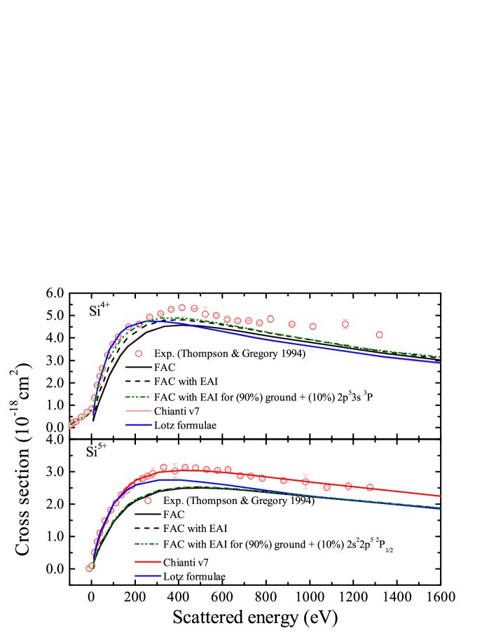
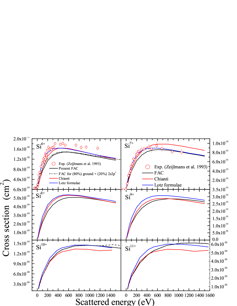
Figure 1.— Cross-section of electron impact ionization for Si⁴⁺ — Si¹¹⁺ ions at their ground stages from different calculations and database along with available experimental data for Si⁴⁺–Si⁷⁺ ions. [A color version of this figure is available in online journal]

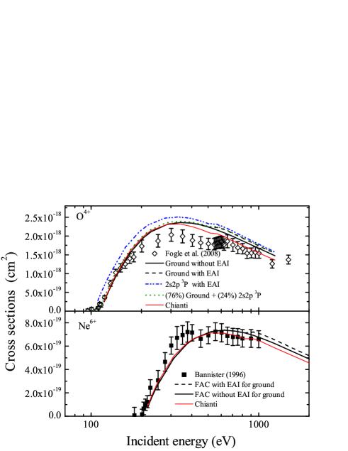
Figure 2.— Comparison of the cross-section of electron impact ionization between the present FAC calculations and experimental measurements by Fogle et al. (2008) and  Bannister (1996) for O⁴⁺  and Ne⁷⁺ ions, respectively. [A color version of this figure is available in online journal]

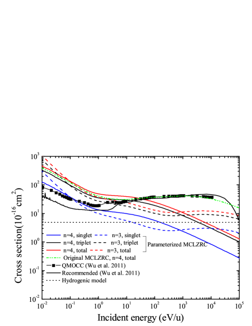
Figure 3.— Comparison of charge exchange cross-section of H-like nitrogen (N⁶⁺) with atomic hydrogen into the $n$=3 and 4 channels. Filled square and solid curve with resonances are the recommend data and molecular-orbital close-coupling calculations from Wu et al. (2011). Horizontal dotted line is from the hydrogenic model that adopted by Wegmann et al. (1997). Solid and dotted curves are from the present parameterized MCLZRC calculation for $n=4$ and 3 channels, respectively. Dashed double-dot line corresponds to the original MCLZRC calculation for $n=4$ channel. [A color version of this figure is available in online journal]

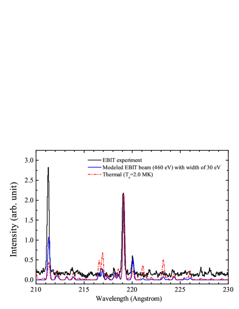
Figure 4.— Theoretical spectra of Fe XIV at thermal ($T_{\rm e}$ = 2.0 MK) and modelled mono-energetic ($E_{\rm e}$ = 460 eV) electrons, along with measurement at Heidelberg EBIT facility (Liang et al., 2010). [A color version of this figure is available in online journal]

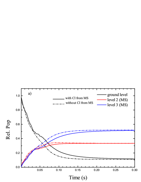
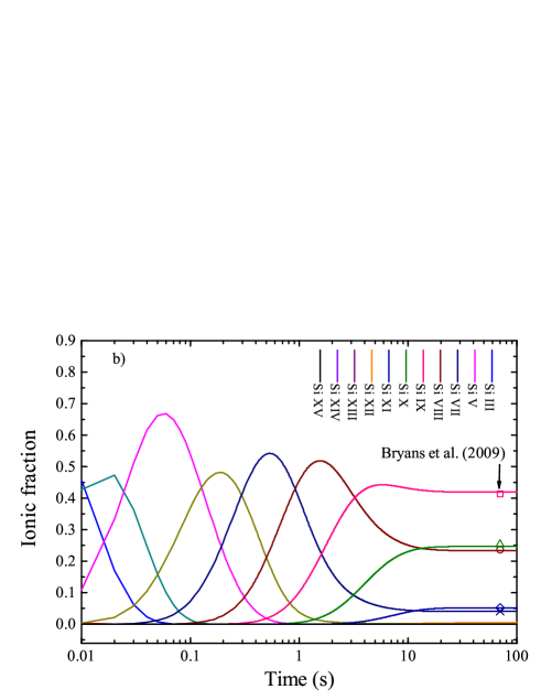
Figure 5.— Time evolution of level population and ionic fraction at an electron density of 10¹⁰ cm^-3. (a) Relative level population of the ground and metastable states (MS, ${\rm 1s^{2}2s^{2}2p^{2}~{}^{3}P_{0,1,2}}$) of Si IX with (solid) and without (dashed-dot) metastable ionization from/to neighbour ions for a modelled electron beam of 500 eV. (b) The fraction of various charged silicon as a function of time (s) at a thermal plasma with temperature of $T_{\rm e}$=1.2 MK. Symbols marked by an arrow correspond to the values of Bryans et al. (2009) at the same temperature. [A color version of this figure is available in online journal]

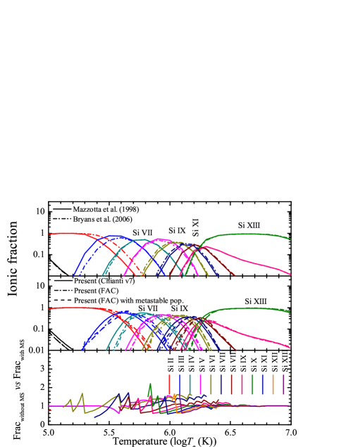
Figure 6.— Ionization balance for highly charged silicon ions (III—XIII) between the temperature range log$T_{\rm e}$ (K)=5–7. Top: Previous data of Mazzotta et al. (1998) and Bryans et al. (2009); Middle: Present calculations by using the Chianti v7 data (solid curves), present FAC calculation data for ionization with (dashed) and without (dashed-dot) metastable populations at electron density of 10¹⁰ cm^-3; Bottom: The ratio of the ionic fractions between the calculation without metastable contributions and that with the metastable contributions.

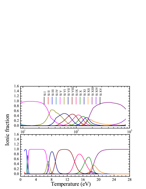
Figure 7.— Charge stage distribution of highly charged silicon ions (I—XV) as a function of thermal temperature (in eV) and radiation field temperature (in eV) in collision (top) and photoionization (bottom) plasmas, respectively. [A color version of this figure is available in online journal]

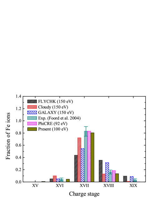
Figure 8.— Comparisons of the predicted ionic fraction of iron ions with the laboratory measurement and previous predictions${}^{\ref{ft_sample}}$ (Foord et al., 2004) from the codes of galaxy, cloudy, flychk and PhiCRE (Wang et al., 2011). [A color version of this figure is available in online journal]

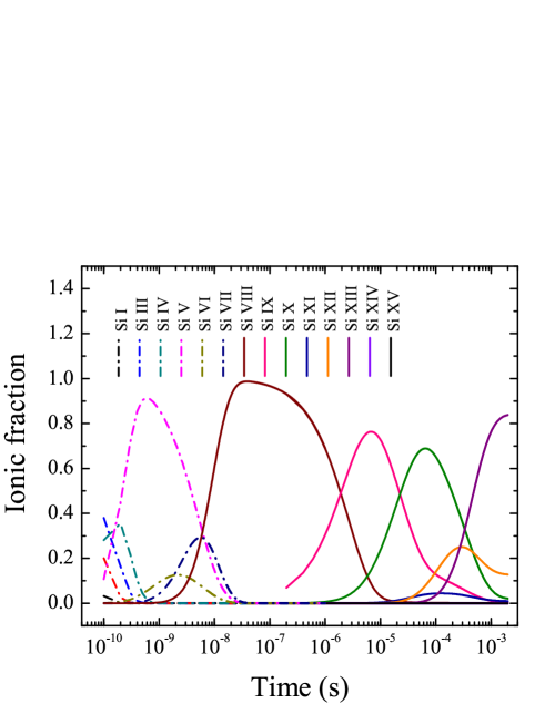
Figure 9.— Time evolution of relative ionic fraction for silicon at an electron density of 10¹⁴ cm^-3 and a radiation source of $T_{\rm r}$=30 eV. [A color version of this figure is available in online journal]

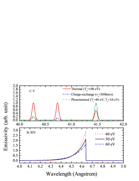
Figure 10.— Top: Spectroscopy of He-like carbon ion ($\lambda_{\rm FWHM}=$ 60 mÅ ) in different plasmas, such as thermal plasma with electron temperature of $T_{\rm e}$=100 eV, photoionized plasma with temperature $T_{\rm r}$=40 eV of Black-body radiation, and geocoronal plasma due to the projection of solar wind ion—C⁵⁺ with velocity of $v_{\rm e}$=200 km/s into cometary or planetary atmosphere with H gas.
Bottom: Radiative recombination continuum of Si XIV at three different temperatures of 40, 50 and 60 eV.

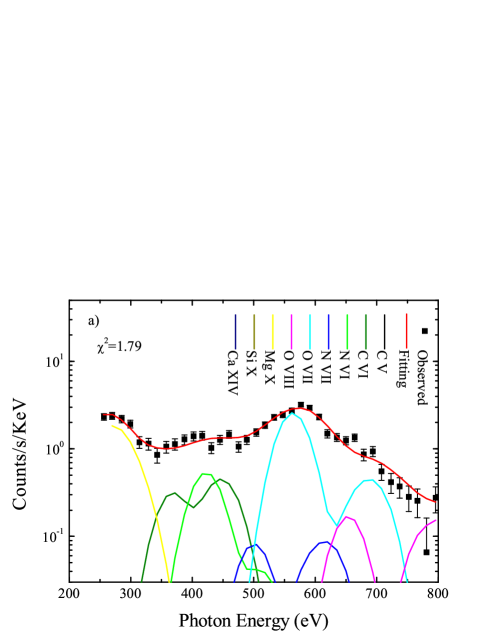
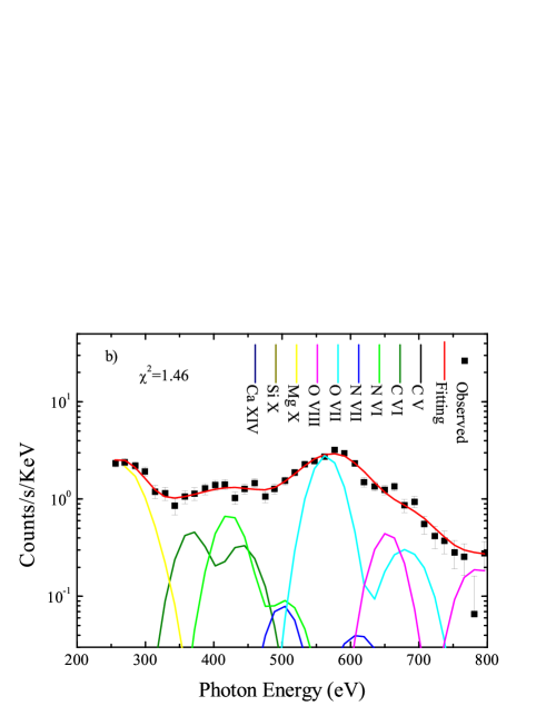
Figure 11.— Co-added Chandra ACIS observation of Linear C/1999 S4 before its breakup on 14 July 2000 and its total fitting performed in Sherpa with line-width of 50 eV at different solar wind velocity of 300 km/s (-a) and 600 km/s (-b), respectively. Specie’s contributions are overlapped by multiplying their CXE model spectra by their fitted fractions. [A color version of this figure is available in online journal]

References

- Abdel-Naby et al. (2012) Abdel-Naby, Sh. A., Nikolć, D., Gorczyca, T.W., et al. 2012, A&A, 537, A40
- Acton et al. (1985) Acton, L.W., Bruner, M.E., Brown, et al. 1985, ApJ, 291, 865
- Altun et al. (2004) Altun, Z., Yumak, A., Badnell, N.R., et al. 2004, A&A, 420, 775
- Altun et al. (2006) Altun, Z., Yumak, A., & Badnell, N.R. 2006, A&A, 447, 1165
- Altun et al. (2007) Altun, Z., Yumak, A., Yavuz, I., et al. 2007, A&A, 474, 1051
- Badnell (1986) Badnell, N.R. 1986, J. Phys. B: At. Mol. Opt. Phys., 19, 3827
- Badnell (2006a) Badnell, N.R. 2006a, ApJS, 167, 334
- Badnell (2006b) Badnell, N.R. 2006b, A&A, 447, 389
- Badnell et al. (2003) Badnell, N.R., O’Mullane, M.G., Summers, H.P., et al. 2003, A&A, 406, 1151
- Bannister (1996) Bannister, M.E. 1996, Phys. Rev. A, 54, 1435
- Bautista & Badnell (2006) Bautista, M.A., & Badnell, N.R. 2006, A&A, 466, 755
- Beiersdorfer (2003) Beiersdorfer, P. 2003, Ann. Rev. Astron. Astrophys., 41, 343
- Beiersdorfer et al. (2003) Beiersdorfer, P., Boyce, K.R., Brown, G.V., et al. 2003, Science, 300, 1558
- Beiersdorfer & Lepson (2012) Beiersdorfer, P., & Lepson, J.K. 2012, ApJS, 201, 28
- Bradshaw & Cargill (2010) Bradshaw, S.J., & Cargill, P.J. 2010, ApJ, 717, 163
- Brosius et al. (2000) Brosius, J.W., Thomas, R.J., Davila, J.M., et al. 2000, ApJ, 543, 1016
- Bryans et al. (2009) Bryans, P., Landi, E., & Savin, D.W. 2009, ApJ, 691, 1540
- Bodewits et al. (2007) Bodewits, D., Christian, D.J., Torney, M., et al. 2007, A&A, 469, 1183
- Butler & Dalgarno (1980) Butler, S.E., & Dalgarno, A. 1980, ApJ, 241, 838
- Colgan et al. (2004) Colgan, J., Pindzola, M.S., & Badnell, N.R. 2004, A&A, 417, 1183
- Colgan et al. (2003) Colgan, J., Pindzola, M.S., Whiteford, A.D., et al. 2003, A&A, 412, 597
- Cravens (1997) Cravens, T.E. 1997, Geophys. Res. Lett., 24, 105
- Del Zenna & Woods (2013) Del Zanna, G., & Woods, T.N. 2003, A&A, 555, A59
- Dere (2007) Dere, K.P. 2007, A&A, 466, 771
- Dickson (1993) Dickson, W.J. 1993, PhD dissertation, University of Strathclyde
- Ferland et al. (1998) Ferland, G.J., Korista, K.T., Verner, D.A., et al. 1998, PASP, 110, 761
- Fogle et al. (2008) Fogle, M., Bahati, E.M., Bannister, M.E., et al. 2008, ApJS, 175, 543
- Foord et al. (2004) Foord, M.E., Heeter, R.F., van Hoof, P.A.M., et al. 2004, Phys. Rev. Lett., 93, 055002
- Fournier et al. (2001) Fournier, K.B., Finkenthal, M., Pacella, D., et al. 2001, ApJ, 550, L117
- Fujioka et al. (2009) Fujioka, S., Takabe, H., Yamamoto, N., et al. 2009, Nature Phys., 5, 821
- Gabriel (1972) Gabriel, A.H. 1972, MNRAS, 160, 99
- Garmire et al. (2003) Garmire, G.P., Bautz, M.W., Ford, P.G., et al. 2003, Proc. SPIE, 4581, 28; doi:10.1117/12.461599
- González Martínez et al. (2006) González Martínez, A.J., Crespo López-Urrutia, J.R., Braun, J., et al. 2006, Phys. Rev. A, 73, 052710
- Gorczyca et al. (2003) Gorczyca, T.W., Kodituwakku, C.N., Korista, K.T., et al. 2003, ApJ, 592, 636
- Gu (2008) Gu, M.F. 2008, Can. J. Phys., 86, 675
- Gdel & Nazé (2009) Gdel, M., & Nazé, Y. 2009, Astron. Astrophys. Rev., 17, 309
- Hberli et al. (2001) Hberli, R.M., Gombosi, T.I., De Zeeuw, D.L., et al. 2001, Science, 276, 939
- Janev et al. (1983) Janev, R.K., Belić, D.S., & Bransden, B.H. 1983, Phys. Rev. A, 28, 1293
- Kallman et al. (2001) Kallman, T., & Bautista, M. 2001, ApJS, 133, 221
- Kallman et al. (2004) Kallman, T.R., Palmeri, P., Bautista, M.A., et al. 2004, ApJS, 155, 675
- Krasnopolsky (2006) Krasnopolsky, V.A. 2006, J. Geophys. Res., 111, A12102
- Landau (1932) Landau, L.D. 1932, Phys. Z., 2, 46
- Landi et al. (2012) Landi, E., Del Zanna, G., Young, P.R., et al. 2012, ApJ, 744, 99
- Li et al. (2013) Li, F., Liang, G.Y., Bari, M.A., et al. 2013, A&A, 556, A32
- Liang & Badnell (2010) Liang, G.Y., & Badnell, N.R. 2010, A&A, 518, A64
- Liang & Badnell (2011) Liang, G.Y., & Badnell, N.R. 2011, A&A, 528, A69
- Liang et al. (2012) Liang, G.Y., Badnell, N.R., & Zhao, G. 2012, A&A, 547, A87
- Liang et al. (2011) Liang, G.Y., Badnell, N.R., Zhao, G., et al. 2011, A&A, 533, A87
- Liang et al. (2010) Liang, G.Y., Badnell, N.R., Crespo López-Urrutia, J.R., et. al. 2010, ApJS, 190, 322
- Liang et al. (2009) Liang, G.Y., Baumann, T.M., Crespo López-Urrutia, J.R., et. al. 2009, ApJ, 696, 2275
- Liang et al. (2009a) Liang, G.Y., Whiteford, A.D., & Badnell, N.R. 2009a, A&A, 500, 1263
- Liang et al. (2009b) Liang, G.Y., Whiteford, A.D., & Badnell, N.R. 2009b, J. Phys. B: At. Mol. Opt. Phys., 42, 225002
- Lisse et al. (2001) Lisse, C.M., Christian, D.J., Dennerl, K., et al. 2001, Science, 292, 1343
- Loch et al. (2009) Loch, S.D., Ballance, C.P., Pindzola, M.S., & Stotler, D.P. 2009, Plasma Phys. Control. Fusion, 51, 105006
- Mazzotta et al. (1998) Mazzotta, P., Mazzitelli, G., Colafrancesco, S. 1998, ApJS, 133, 403
- Mewe et al. (1995) Mewe, R., Kaastra, J.S., & Liedahl, D.A. 1995, Legacy, 6, 16
- Milligan (2011) Milligan, R.O. 2011, ApJ, 740, 70
- Mitnik & Badnell (2004) Mitnik, D.M., & Badnell, N.R. 2004, A&A, 425, 1153
- Nahar et al. (2000) Nahar, S.N., Pradhan, A.K., & Zhang, H.L. 2000, ApJS, 131, 375
- Oelgoetz & Pradhan (2004) Oelgoetz, J., & Pradhan, A.K. 2004, MNRAS, 354, 1093
- Otranto & Olson (2008) Otranto, S., & Olson, R.E. 2008, Phys. Rev. A, 77, 022709
- Otranto et al. (2007) Otranto, S., Olson, R.E., & Beiersdorfer, P. 2007, J. Phys. B: At. Mol. Opt. Phys., 40, 1755
- Paerels et al. (2000) Paerels, F., Cottam, J., Sako, M., et al. 2000, ApJ, 533, L135
- Raymond & Smith (1977) Raymond, J.C., & Smith, B.W. 1977, ApJS, 35, 419
- Remington et al. (2006) Remington, B.A., Drake, R.P., & Ryutov, D.D. 2006, Rev. of Mod. Phys., 78, 755
- Salop & Olson (1976) Salop, A., & Olson, R.E. 1976, Phys. Rev. A, 13, 1312
- Schwadron & Cravens (2000) Schwadron, N.A., & Cravens, T.E. 2000, ApJ, 544, 558
- Shipsey et al. (1983) Shipsey, E.J., Green, T.A., & Browne, J.C. 1983, Phys. Rev. A, 27, 821
- Smith et al. (2001) Smith, R.K., Brickhouse, N.S., Liedahl, D.A., et al. 2001, ApJ, 556, L91
- Smith & Hughes (2010) Smith, R.K., & Hughes, J.P. 2010, ApJ, 718, 583
- Smith et al. (2012) Smith, R.K., Foster, A.R., & Brickhouse, N.S. 2012, Astron. Nachr., 4, 301
- Summers et al. (2006) Summers, H.P., Dickson, W.J., O’Mullane, M.G., et al. 2006, Plasma Phys. Control. Fusion, 48, 263
- Thompson & Gregory (1994) Thompson, J.S., & Gregory, D.C. 1994, Phys. Rev. A, 50, 1377
- Torney (2007) Torney, M. 2007, PhD dissertation, University of Strathclyde
- Tucker & Gould (1966) Tucker, W.H., & Gould, R.J. 1966, ApJ, 144, 244
- Vainshtein & Safronova (1978) Vainshtein, L.A., & Safronova, U.I. 1978, Atom. Data and Nuc. Data Tab., 21, 49
- Vainshtein & Safronova (1980) Vainshtein, L.A., & Safronova, U.I. 1980, Atom. Data and Nuc. Data Tab., 25, 311
- van Kerkwijk et al. (1992) van Kerkwijk, M. H., Charles, P.A., Geballe, T.R., et al. 1992, Nature, 355, 703
- Verner et al. (1996) Verner, D.A., Ferland, G.J., Korista, K.T., & Yakovlev, D.G. 1996, ApJ, 465, 487
- Wang et al. (2011) Wang, F.L., Salzmann, D., Zhao, G., et al. 2011, ApJ, 742, 53
- Wegmann et al. (1997) Wegmann, R., Schmidt, H.U., Lisse, C.M., et al. 1997, Planet. Space Sci., 46, 603
- Whiteford et al. (2001) Whiteford, A.D., Badnell, N.R., Ballance, C.P., et al. 2001, J. Phys. B: At. Mol. Opt. Phys., 34, 3179
- Witthoeft et al. (2007) Witthoeft, M.C., Whiteford, A.D., & Badnell, N.R. 2007, J. Phys. B: At. Mol. Opt. Phys., 40, 2969
- Witthoeft et al. (2009) Witthoeft, M.C., Bautista, M.A., Mendoza, C., et al. 2009, ApJS, 182, 127
- Witthoeft et al. (2011a) Witthoeft, M.C., García, J., Kallman, T.R., et al. 2011a, ApJS, 192, 7
- Witthoeft et al. (2011b) Witthoeft, M.C., Bautista, M.A., García, J., et al. 2011b, ApJS, 196, 7
- Wu et al. (2011) Wu, Y., Stancil, P.C., Liebermann, H.P., et al. 2011, Phys. Rev. A, 84, 022711
- Zatsarinny et al. (2006) Zatsarinny, O., Gorczyca, T.W., Fu, J., et al. 2006, A&A, 447, 379
- Zatsarinny et al. (2003) Zatsarinny, O., Gorczyca, T.W., Korista, K.T., et al. 2003, A&A, 412, 587
- Zatsarinny et al. (2004a) Zatsarinny, O., Gorczyca, T.W., Korista, K.T., et al. 2004a, A&A, 417, 1173
- Zatsarinny et al. (2004b) Zatsarinny, O., Gorczyca, T.W., Korista, K.T., et al. 2004b, A&A, 426, 699
- Zeijlmans et al. (1993) Zeijlmans van Emmichoven, P.A., Bannister, M.E., Gregory, D.C., et al. 1993, Phys. Rev. A, 47, 2888
- Zener (1932) Zener, C. 1932, Proc. R. Soc. London A, 137, 696
- Zhang & Sampson (1990) Zhang, H.L., & Sampson, D.H. 1990, Phys. Rev. A, 42, 5378
- Zhong et al. (2010) Zhong, J.Y., Li, Y.T., Wang, X.G., et al. 2010, Nature Phys., 6, 984