Transversal instability for the thermodiffusive reaction-diffusion system

Abstract

The propagation of unstable interfaces is at the origin of remarkable patterns that are observed in various areas of science as chemical reactions, phase transitions, growth of bacterial colonies. Since a scalar equation generates usually stable waves, the simplest mathematical description relies on two by two reaction-diffusion systems. Our interest is the extension of the Fisher/KPP equation to a two species reaction which represents reactant concentration and temperature when used for flame propagation, bacterial population and nutrient concentration when used in biology.

We study in which circumstances instabilities can occur and in particular the effect of dimension. It is observed numerically that spherical waves can be unstable depending on the coefficients. A simpler mathematical framework is to study transversal instability, that means a one dimensional wave propagating in two space dimensions. Then, explicit analytical formulas give explicitely the range of paramaters for instability.

Key-words: Traveling waves; Stability analysis; Reaction-diffusion equation; Thermodiffusive system.
Mathematical Classification numbers: 35C07; 70K50; 76E17; 80A25; 92C17

1 Introduction

The propagation of unstable interfaces is at the origin of remarkable patterns that can be observed in nature and in experiments. The phenomena has attracted the attention of physicists, geophysicists, chemists and biologists and basic mathematical models can account for this type of unstable dynamical patterns. These models are reaction-diffusion systems and the simplest model is an extension of the Fisher/KPP equation to a two species reaction. It models reactant concentration and temperature when used for flame propagation [3, 5], bacterial population and nutrient concentration when used in biology [13, 8], cancer cells and available oxygen/glucosis when used for tumor growth [2, 16, 14].

Numerical simulations show that spherical waves can be unstable or stable depending on the model coefficients. But among the many scenarios of instability, the so-called ‘transversal instabilities’ are the simplest to analyze and explain this surprising effect of dimension which is to de-stabilize a stable one dimensional traveling wave. The phenomena was observed and related to Diffusion Limited Aggregation, with a first analysis, in [11, 18].

Our goal here is to study such a case of transversal instability and more precisely to understand the modalities of appearance of transversal instabilities for a very simple example given by system. For this, we consider the following two-component reaction-diffusion system :

$$\left\{\begin{array}[]{l}\partial_{t}u-\alpha\Delta u=\frac{1}{\alpha}h(u)v,\\[5.69054pt] \partial_{t}v-\Delta v=-\frac{1}{\alpha}h(u)v.\end{array}\right.$$ (1)

The parameter $\alpha>0$ is called the Lewis number for flame propagation theory, $\alpha>1$ is relevant for combustion and $\alpha<1$ is more relevant for applications to bacterial movement.

Two different cases are proposed both for combustion and biology litteratures depending on propertie of the function $h(\cdot)$

$$h\in C^{1}(0,1),\qquad h(0)=0,\qquad h(1)=1,\qquad h^{\prime}(u)>0\quad\text{for }\;0<u\leq 1,\qquad\text{(KPP type)},$$

$$\begin{cases}h(u)=0\quad\text{for }\;0\leq u\leq\theta<1,\qquad h(\theta+)=h^{+}\geq 0,\\[5.69054pt] h(1)=1,\quad h^{\prime}(u)\geq 0\quad\text{for }\;\theta<u\leq 1,\end{cases}\qquad\text{(Ignition temperature type).}$$

Our interest lies on two dimensional stability of one dimensional traveling waves for this system. A proof of existence for one dimensional traveling wave solutions can be found in [12] when $h(\cdot)$ is of KPP type and when $\alpha\geq 1$ for ignition temperature type. Also, in [3], the authors prove existence of traveling waves when $h(\cdot)$ is of ignition temperature type and no restriction on $\alpha$. More recent results for KPP type, in a cylinder and covering all Lewis numbers, can be found in [9].

In this paper, we consider a simple example for which we can handle analytical computation. It corresponds to ignition temperature type and the function $h$ is given by

$$h(u)=\left\{\begin{array}[]{l}0,\qquad\mbox{for }u\leq\theta,\\ 1,\qquad\mbox{for }u>\theta.\end{array}\right.$$ (2)

We first report in Section 2, based on numerical simulations, two dimensional spherical waves which can be unstable for certain coefficients. Then, we build analytically the one dimensional traveling waves in Section 3. The analytical formulas are fundamental to handle the spectral problem arising to study linearized stability of the transversal waves in Section 4.

2 Numerical observations

In two dimensions, numerical simulations of system (1)–(2) exhibit various behaviours depending on the values of $\alpha$ and $\theta$ in $(0,1)$. We present them here as a motivation for our theoretical study.

These simulations are obtained using the finite element method implemented within the software FreeFem++ [1, 10]. The computational domain is a disc with radius $4$ and we denote by $\Gamma$ its boundary. At the boundary, Neumann boundary conditions are implemented for both $u$ and $v$ :

$$\partial_{\nu}u|_{\Gamma}=0,\qquad\partial_{\nu}v|_{\Gamma}=0,$$

where $\nu$ is the outward unit normal. We use a semi-implicit time discretization. Then the resulting system is discretized thanks to P1 finite element method.

The initial given data is :

$$u^{0}={\bf 1}_{\{\sqrt{x^{2}+y^{2}}\leq 0.4\}};\qquad v^{0}=1-u^{0}.$$

The time step is $dt=0.0025$ and the number of nodes is $21879$. The numerical results are depicted in Figure 1 and 2 where the computed approximation of $u$ is plotted after several time iterations for different values of the parameters $\alpha$ and $\theta$. Depending on the values of $\alpha$ and $\theta$, we observe different patterns in the numerical simulations. Figure 1 displays the numerical simulations for $\alpha=0.25$ and for $\theta=0.1$ (Left) and $\theta=0.5$ (Right). In both cases, we observe a wave that invades the computational domain and the numerical result do not show instabilities. Comparing this two results, we deduce that the invasion process depends on $\theta$. Figure 2 displays the numerical results obtained for small $\alpha$ : we choose $\alpha=0.01$. In this case, we observe numerical instabilities that create a complex pattern. Instabilities are much more visible when $\theta=0.1$ (Figure 2, Left) than when $\theta=0.5$ (Figure 2, Right).

   

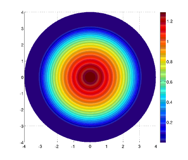
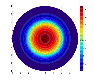
Figure 1: Numerical simulations for component $u$ in (1). (1) Left: Plot of the computed $u$ at time $T=1$ for $\alpha=0.25$ and $\theta=0.1$. (2) Right: Plot of the computed $u$ at time $T=3$ for $\alpha=0.25$ and $\theta=0.5$. In both cases, we observe the propagation of a stable spherical wave which invades the computational domain.

   

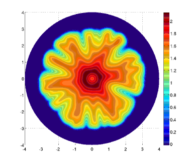
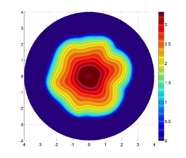
Figure 2: Numerical simulations for species $u$ in (1). (1) Left: Plot of the computed $u$ at time $T=2$ for $\alpha=0.01$ and $\theta=0.1$. (2) Right: Plot of the computed $u$ at time $T=6$ for $\alpha=0.25$ and $\theta=0.5$. When $\alpha$ is small, numerical instabilities appear which create a complex fingered pattern.

3 One dimensional traveling waves

One dimensional traveling waves are solutions of the form

$$u(t,x)=u_{0}(x-\sigma t),\quad v(t,x)=v_{0}(x-\sigma t),$$

where $\sigma>0$ is a constant representing the traveling wave velocity. They are a convenient way to understand the propagation phenomena presented in Section 2.

For system (1) traveling waves are determined from the system :

$$\left\{\begin{array}[]{l}-\sigma{u_{0}}_{x}-\alpha{u_{0}}_{xx}=\frac{1}{\alpha}h(u_{0})v_{0},\\[5.69054pt] -\sigma{v_{0}}_{x}-{v_{0}}_{xx}=-\frac{1}{\alpha}h(u_{0})v_{0},\\[5.69054pt] (u_{0},v_{0})(-\infty)=(1,0),\qquad(u_{0},v_{0})(+\infty)=(0,1).\end{array}\right.$$ (3)

To avoid ambiguity due to the translation invariance of the problem we set

$$0<u_{0}(0)=\theta<1.$$ (4)

We say that a traveling wave solution to (3) is monotonic, if each component is monotonic, and then we can normalize the signs with $u_{0}^{\prime}<0$ and $v_{0}^{\prime}>0$.

Proposition 3.1

There exists a unique monotonic traveling wave for system (1)–(2), i.e. a unique $\sigma>0$ and a pair $(u_{0},v_{0})\in\mathcal{C}^{1,\nu}(\mathbb{R})$, $\nu\in(0,1)$, solving (3)–(4) with $u_{0}$ nonincreasing, $v_{0}$ nondecreasing.

More precisely this traveling wave solution moves with the speed

$$\sigma=(1-\theta)\sqrt{\frac{\alpha}{\theta^{2}+\alpha\theta(1-\theta)}}$$ (5)

and is given explicitly by

$$u_{0}(x)=\left\{\begin{array}[]{ll}1-(1-\theta)e^{\theta x/\beta},&\mbox{ for }x<0,\\[5.69054pt] \theta e^{-(1-\theta)x/\beta},&\mbox{ for }x>0,\end{array}\right.$$ (6)

$$v_{0}(x)=\left\{\begin{array}[]{ll}\frac{\alpha(1-\theta)}{\theta+\alpha(1-\theta)}e^{\theta x/\beta},&\mbox{ for }x<0,\\[5.69054pt] 1-\frac{\theta}{\theta+\alpha(1-\theta)}e^{-\alpha(1-\theta)x/\beta},&\mbox{ for }x>0,\end{array}\right.$$ (7)

where

$$\beta=\sqrt{\alpha\theta}\,\sqrt{\theta+\alpha(1-\theta)}.$$ (8)

This solution is depicted in Figure 3.

Remark 3.2

We notice that when $\theta$ goes to $0$, we have that $\sigma\sim\frac{\sqrt{\alpha}}{\theta}$. Then the wave goes faster when $\theta$ is smaller. This remark confirms our observation in Figure 1, where we can notice than the invasion process of species $u$ is faster when $\theta$ is smaller.

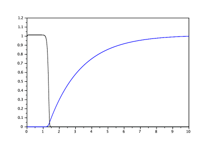
Figure 3: The traveling wave solution with $u$ decreasing and $v$ increasing for $\alpha=0.005$ and $\theta=0.1$.

Proof. We recall that we look for a nonincreasing function $u$ and we have denoted $u_{0}(0)=\theta$. Therefore, from the definition of the nonlinearity $h(\cdot)$ in (2), we have $h\big{(}u_{0}(x)\big{)}=0$ for $x>0$. Then, the system (3) is reduced to

$$-\sigma{u_{0}}_{x}-\alpha{u_{0}}_{xx}=0,\qquad-\sigma{v_{0}}_{x}-{v_{0}}_{xx}=0,\qquad x>0.$$

With the boundary condition at $+\infty$ in (3) : $(u_{0},v_{0})(+\infty)=(0,1)$, we deduce

$$u_{0}(x)=\theta e^{-\sigma x/\alpha},\qquad v_{0}(x)=1-be^{-\sigma x},\qquad\mbox{ for }x>0,$$ (9)

where $b$ is a constant to be fixed later.

For $x<0$, we have $h\big{(}u_{0}(x)\big{)}=1$, therefore system (3) is reduced to

$$-\sigma{u_{0}}_{x}-\alpha{u_{0}}_{xx}=\frac{v_{0}}{\alpha},\qquad\sigma{v_{0}}_{x}+{v_{0}}_{xx}-\frac{1}{\alpha}v_{0}=0.$$

Solving the second equation, and because the solution is continuous at $x=0$ by ellipitic regularity, leads to

$$v_{0}(x)=(1-b)e^{\lambda x},\qquad\mbox{ with }\quad\lambda=\frac{1}{2}\big{(}-\sigma+\sqrt{\sigma^{2}+4/\alpha}\big{)},\qquad\mbox{ for }x<0,$$ (10)

where we have used the boundary conditions : $(u_{0},v_{0})(-\infty)=(1,0)$. Then, we obtain

$$u_{0}(x)=1-(1-\theta)e^{\lambda x},\qquad\mbox{ for }x<0,$$ (11)

which is a solution of the equation for $u_{0}$ provided

$$\big{(}\sigma\lambda+\alpha\lambda^{2}\big{)}(1-\theta)=\frac{1-b}{\alpha}.$$

This latter equality allows to determine the value of $b$ :

$$b=1-\alpha\big{(}1+\sigma\lambda(1-\alpha)\big{)}(1-\theta).$$

Finally, the continuity of the derivative $u^{\prime}_{0}(0^{+})=u^{\prime}_{0}(0^{-})$ implies $\displaystyle\frac{\sigma\theta}{\alpha}=\lambda(1-\theta).$ Using this relation and the expression of $\lambda$ (10) we obtain

$$\sigma=(1-\theta)\sqrt{\frac{\alpha}{\theta^{2}+\alpha\theta(1-\theta)}}.$$

We deduce

$$\lambda=\frac{\sqrt{\theta}}{\sqrt{\alpha}\sqrt{\theta+\alpha(1-\theta)}},\qquad\sigma\lambda=\frac{1-\theta}{\theta+\alpha(1-\theta)},\qquad b=\frac{\theta}{\theta+\alpha(1-\theta)}.$$ (12)

The conclusions stated in Proposition 3.1 follow directly from the construction and formulas (9)–(10)–(11).       

4 Stability of planar traveling waves

As suggested by the numerical results in Section 2, based on spherical waves, we expect that transversal instability can occur in two dimensions.

We propose here to study the linear transversal stability. To do so, and in the spirit of [11, 7] for instance, with $\varepsilon\ll 1$, we set

$$\left\{\begin{array}[]{l}u(t,x,y)=u_{0}(x-\sigma t)+\varepsilon e^{\lambda t}\cos(\omega y)u_{1}(x-\sigma t),\\[5.69054pt] v(t,x,y)=v_{0}(x-\sigma t)+\varepsilon e^{\lambda t}\cos(\omega y)v_{1}(x-\sigma t).\end{array}\right.$$

Substituting this expansion into (1) and keeping only the term of order 1 in $\varepsilon$, we get the linearized system (in the traveling wave frame)

$$\left\{\begin{array}[]{l}\lambda u_{1}-\sigma u_{1}^{\prime}-\alpha u_{1}^{\prime\prime}+\alpha\omega^{2}u_{1}=\frac{1}{\alpha}\big{(}h^{\prime}(u_{0})v_{0}u_{1}+h(u_{0})v_{1}\big{)},\\[5.69054pt] \lambda v_{1}-\sigma v^{\prime}_{1}-v_{1}^{\prime\prime}+\omega^{2}v_{1}=-\frac{1}{\alpha}\big{(}h^{\prime}(u_{0})v_{0}u_{1}+h(u_{0})v_{1}\big{)}.\end{array}\right.$$ (13)

We notice that for $\omega=0$, the system has the solution $\lambda=0$, $u_{1}=u^{\prime}_{0}$ and $v_{1}=v^{\prime}_{0}$. Notice that $\omega=0$ also represents the case of dimension one (no transversal effect)s.

Definition 4.1

In two dimensions, we say that the one dimensional traveling wave $(u_{0},v_{0})$ for system (1) in Proposition 3.1 is transversally linearly unstable if there exists $\omega>0$ and $\lambda$ with $\mathrm{Re}\,\lambda>0$ such that system (13) admits a non-trivial solution in $\mathcal{C}^{\nu}(\mathbb{R})\cap L^{2}(\mathbb{R})$.

Proposition 4.2

Let $\theta\in(0,1)$. Let us consider the function $h$ given in (2). Then the following hold:

1. For $\alpha$ small enough, the traveling waves in Proposition 3.1 are linearly stable in one dimension for all $\theta\in(0,1)$.

2. For each $\theta\in(0,1)$ and each small $\alpha$ there exists $\omega(\alpha,\theta)$ such that $\lambda(\omega(\alpha,\theta))<0$ i.e. the traveling wave is transversally linearly unstable for these values of the parameters in two dimensions. Moreover $\omega(\alpha,\theta)=\mathcal{O}(\frac{1}{\sqrt{\alpha}})$.

The paper [15] suggests that, in appropriate weighted spaces, one dimensional traveling wave are nonlinearly stable in the range of parameters when they are linearly stable.

Proof. Since linear stability in one dimension reduces to studying (13) for $\omega=0$, from now on we assume more generally that $\omega\geq 0$. We will look for $\lambda\in\mathbb{R}$, $\lambda=\lambda(\omega)>0$ such that system (13) admits a non-trivial solution. Note that $\lambda$ depends on $\alpha$ and $\theta$ as well, but we will not make this dependence explicit unless necessary.

For $x>0$, system (13) reduces to

$$\left\{\begin{array}[]{l}(\alpha\omega^{2}+\lambda)u_{1}-\frac{(1-\theta)\alpha}{\beta}u^{\prime}_{1}-\alpha u^{\prime\prime}_{1}=0,\\[5.69054pt] (\lambda+\omega^{2})v_{1}-\frac{(1-\theta)\alpha}{\beta}v^{\prime}_{1}-v^{\prime\prime}_{1}=0.\end{array}\right.$$

We can solve this linear problem and obtain

$$\left\{\begin{array}[]{l}u_{1}(x)=Ae^{r_{-}x},\qquad r_{-}=-\frac{(1-\theta)}{2\beta}-\frac{1}{2\beta}\sqrt{(1-\theta)^{2}+4\beta^{2}(\omega^{2}+\frac{\lambda}{\alpha})},\\[5.69054pt] v_{1}(x)=Be^{s_{-}x},\qquad s_{-}=-\frac{(1-\theta)\alpha}{2\beta}-\frac{1}{2\beta}\sqrt{(1-\theta)^{2}\alpha^{2}+4\beta^{2}(\omega^{2}+\lambda)}.\end{array}\right.$$ (14)

Here, $A$ and $B$ are constants to be determined and $r_{\pm}$ are the roots of the polynomial

$$(\alpha\omega^{2}+\lambda)-\frac{(1-\theta)\alpha}{\beta}r-\alpha r^{2}=0.$$ (15)

For $x<0$, system (13) reduces to

$$\left\{\begin{array}[]{l}(\alpha\omega^{2}+\lambda)u_{1}-\frac{(1-\theta)\alpha}{\beta}u^{\prime}_{1}-\alpha u^{\prime\prime}_{1}=\frac{1}{\alpha}v_{1},\\[5.69054pt] \Big{(}\lambda+\omega^{2}+\frac{1}{\alpha}\Big{)}v_{1}-\frac{(1-\theta)\alpha}{\beta}v^{\prime}_{1}-v^{\prime\prime}_{1}=0,\end{array}\right.$$

where we have used the expression of $\sigma$ in (5) recalling that $\beta$ is given in (8). Then we get

$$v_{1}(x)=Be^{\mu_{+}x},\qquad\mu_{+}=-\frac{(1-\theta)\alpha}{2\beta}+\frac{1}{2\beta}\sqrt{(2\theta+\alpha(1-\theta))^{2}+4\beta^{2}(\omega^{2}+\lambda)}.$$ (16)

Substituting this expression in the equation for $u_{1}$, we get

$$u_{1}(x)=Ce^{r_{+}x}+\gamma Be^{\mu_{+}x},\qquad r_{+}=-\frac{(1-\theta)}{2\beta}+\frac{1}{2\beta}\sqrt{(1-\theta)^{2}+4\beta^{2}(\omega^{2}+\frac{\lambda}{\alpha})},\\$$ (17)

where $C$ is a constant and we have set

$$\Big{(}\alpha\omega^{2}+\lambda-\frac{(1-\theta)\alpha}{\beta}\mu_{+}-\alpha\mu_{+}^{2}\Big{)}\gamma=\frac{1}{\alpha}.$$

The value of the parameter $\gamma$ follows from the definition of $r_{\pm}$ as the roots of (15)

$$\gamma=-\frac{1}{\alpha^{2}(\mu_{+}-r_{+})(\mu_{+}-r_{-})}.$$ (18)

Moreover, by continuity at $x=0$, we need $C+B\gamma=A$. By definition of the function $h$ and with (6)–(7), we obtain

$$h^{\prime}(u_{0})v_{0}=\frac{\beta\alpha}{\theta(\theta+\alpha(1-\theta))}\delta_{x=0}=\frac{\alpha^{2}}{\beta}\delta_{x=0}.$$ (19)

As a consequence, the jump relation for $(u^{\prime}_{1},v_{1}^{\prime})$ at $x=0$, which can be deduced from equation (13), leads to

$$\left\{\begin{array}[]{l}-\alpha(u^{\prime}_{1}(0^{+})-u^{\prime}_{1}(0^{-}))=\frac{\alpha}{\beta}u_{1}(0),\\[5.69054pt] -v^{\prime}_{1}(0^{+})+v^{\prime}_{1}(0^{-})=-\frac{\alpha}{\beta}u_{1}(0).\end{array}\right.$$

Writing these equalities in terms of the free parameters, we arrive to the following set of relations

$$\left\{\begin{array}[]{l}A=C+\gamma B,\\[5.69054pt] A\big{(}r_{-}+\frac{1}{\beta}\big{)}=Cr_{+}+\gamma\mu_{+}B,\\[5.69054pt] \frac{\alpha}{\beta}A=Bs_{-}-B\mu_{+}.\end{array}\right.$$

Replacing $B$ and $C$ in the second equation, we get

$$A\big{(}r_{-}+\frac{1}{\beta}\big{)}=Ar_{+}+A\gamma(\mu_{+}-r_{+})\frac{\alpha}{\beta(s_{-}-\mu_{+})}.$$

We conclude that there exists a non trivial solution to (13) provided the following identity holds :

$$1=\beta(r_{+}-r_{-})+\frac{1}{\alpha(\mu_{+}-r_{-})(\mu_{+}-s_{-})},$$ (20)

where we used the expression (18). We verify straightforwardly that for $\omega=0$ and $\lambda=0$ relation (20) is always satisfied.

It remains to compute the value of $\lambda$ using (20). In this algebraic equation $\lambda$ is given implicitly as a function of the parameters $\alpha,\theta$ and $\omega$, and in the analysis of this expression we rely on taking the limit $\alpha\to 0$ and also on Maple based simulations (in this sense our proof is to some small extent computer assisted).

First, we consider the case $\omega=0$ which provides the stability in one dimension. Then we consider the limit $\alpha\to 0$ choosing the scale: $\omega=\frac{\omega_{0}}{\sqrt{\alpha}}$, with $\omega_{0}>0$ fixed.

Case 1: $\alpha\to 0$, $\omega=0$. This case covers Assertion 1 of the propostion. We set

$$\zeta=\sqrt{(1-\theta)^{2}+4\beta^{2}\lambda/\alpha},\qquad\eta=\sqrt{(2\theta+\alpha(1-\theta))^{2}+4\beta^{2}\lambda}.$$

Using (14), (16), (17), the identity (20) in the case $\omega=0$ reduces to

$$1=\zeta+\frac{4\beta^{2}}{\alpha\big{(}(1-\theta)(1-\alpha)+\zeta+\eta\big{)}(\eta+\alpha\zeta)}.$$ (21)

Taking $\alpha=0$ above, we find that

$$\lambda=-\frac{1}{2}\,\frac{1-\theta}{\theta}.$$

By continuity, this means in particular that for all sufficiently small $\alpha$, the traveling wave solution is linearly stable. Hence, it is tempting to speculate that in fact linear stability is true for any $\alpha>0$, see however Remark 5.2.

Case 2: $\alpha\to 0$ and $\omega=\frac{\omega_{0}}{\sqrt{\alpha}}$. Calculations are quite similar in this case. Denoting now

$$\zeta=\sqrt{(1-\theta)^{2}+4\theta^{2}(\lambda+\omega^{2}_{0})},$$

we need to solve

$$1-\zeta=\frac{2\theta}{(\sqrt{\omega_{0}^{2}+1}+\omega_{0})(1-\theta+2\theta\sqrt{\omega_{0}^{2}}+\zeta)}.$$

Therefore,

$$\zeta=\frac{1}{2}\left(\theta-2\theta\sqrt{\omega_{0}^{2}+1}+\sqrt{\Big{(}\theta-2\theta\sqrt{\omega_{0}^{2}+1}\Big{)}^{2}+4-4\theta+8\theta\omega_{0}}\right)$$

and then

$$\lambda=-\omega_{0}^{2}+\frac{1}{16\theta^{2}}\Big{(}\theta-2\theta\sqrt{\omega_{0}^{2}+1}+\sqrt{(\theta-2\theta\sqrt{\omega_{0}^{2}+1})^{2}+4-4\theta+8\theta\omega_{0}}\Big{)}^{2}-\Big{(}\frac{1-\theta}{2\theta}\Big{)}^{2}.$$

In this case, depending on the value of $\omega_{0}$ we may have $\lambda>0$ or $\lambda<0$. Figure 4 illustrates the situation.

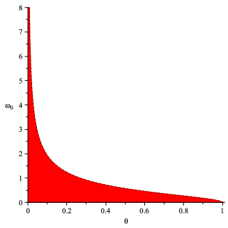
Figure 4: Plot of the region of instability $\lambda=\lambda(\theta,\omega_{0})>0$, marked red.

      

5 Concluding remarks

Remark 5.1

It has been noted with the numerical simulations of Section2, that for small values of $\alpha$, instabilities are more visible when $\theta$ is small (see Figure 2). The plot of the region of instability in Figure 4 confirms this observation. In fact, we notice on this latter Figure that small values of $\theta$ allows large values of $\omega_{0}$ which can be seen as a frequence of oscillations in the transversal direction.

Remark 5.2

We use formula (21) and denote

$$F(\alpha,\theta,\lambda)=\zeta+\frac{4\beta^{2}}{\alpha\big{(}(1-\theta)(1-\alpha)+\zeta+\eta\big{)}(\eta+\alpha\zeta)}-1.$$

Solutions of $F(\alpha,\theta,\lambda)=0$ determine the eigenvalues $\lambda=\lambda(\alpha,\theta)$. It is easy to check that

$$\lim_{\alpha\to\infty}F(\alpha,\theta,\lambda)=\infty,\quad\forall\lambda>0,\;\theta\in(0,1),$$

however this limit is not uniform. Indeed there exist a $\theta^{*}$ such that for any $\theta\in(\theta^{*},1)$ we can find a value $\alpha(\theta)>0$ such that $F(\alpha,\theta,\lambda)=0$ for some $\lambda>0$. We illustrate this in Figure 5.

   

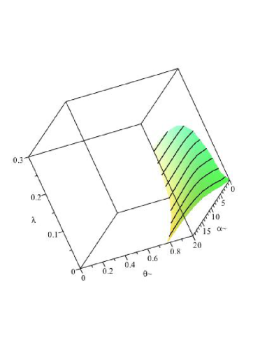
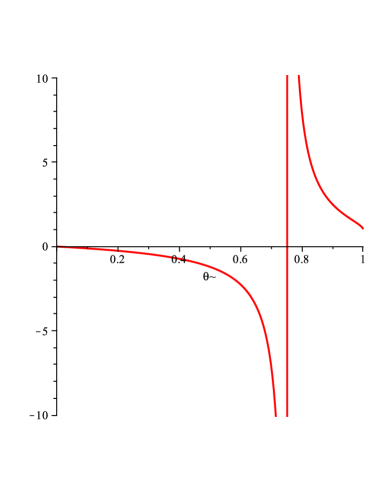
Figure 5: (Left) Plot of the level set $F(\alpha,\theta,\lambda)=0$. (Right) Plot of the implicitly defined curve $\theta\mapsto\alpha(\theta)$ where $F(\alpha(\theta),\theta,0)=0$. It suggests that the instability appears for some $\theta^{*}\in(0.7,0.8)$ and the corresponding values of $\alpha$ are larger than $1$. This is confirmed by a more refined analysis of the picture on the right.

The fact that the traveling wave in one dimension is unstable for large values of the Lewis number is somewhat of a surprise and raises a more general question of stability or instability for the problems with KPP type or ignition type nonlinearities. Note that, in both cases, we are dealing with a prey-predator system and in particular the linear problem is non-cooperative. This means that methods based on maximum principle do not work and the known results (see for instance [19])) do not apply. The special feature of our problem is the monotonicity of the traveling fronts. With this property, one may expect that they should be stable, as it happens for scalar problems and is seen easily there from the Krein-Rutman theorem. For systems of equations, there is no general theory that one could apply but monotone waves are stable in some cases (see for instance [4]). Our example shows that the question is in fact more subtle.

Remark 5.3

Writing (20) in the form

$$0=-1+\beta(r_{+}-r_{-})+\frac{1}{\alpha(\mu_{+}-r_{-})(\mu_{+}-s_{-})},$$

we obtain a dispersion relation $\lambda=\lambda(\omega)$ for any fixed $\alpha$ and $\theta$. Pictures in Figure 6, confirm the intuitively obvious fact that there should always be the most unstable frequency $\omega^{*}$, that is a maximum value of $\lambda$ and this is relevant of Turing instability.

   

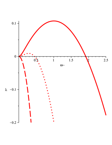
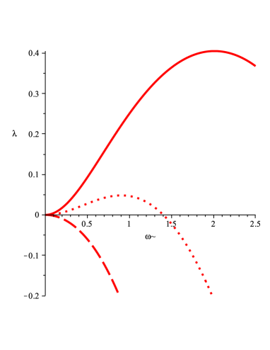
Figure 6: (Left) Plot of the dispersion curve $\lambda(\omega)$ for $\theta=0.4$ and $\alpha=0.1$ (continuous line), $\alpha=0.4$ (dotted line) and $\alpha=1.3$ (dashed line). (Right) Plot of the dispersion curve for $\theta=0.1$ and $\alpha=0.1$ (continuous line) $\alpha=0.2$ (dotted line) $\alpha=0.4$ (dashed line).

The intention of this note is to shed some light on the mechanism of the onset of instability of traveling waves in higher dimension, and in particular to get some idea about the shape of the dispersion curves for more general problems of KPP and ignition type. We chose to study the planar waves for a simple problem where explicit solutions are available since, unlike for example in the case of some activator-inhibitor systems (see [18, 17, 6]), there does not seem to exist a well established methodology to deal with this issue. Indeed, the usual approach, involving some limit procedure, is based on the fact that of one of the components of the system becomes more concentrated in space, for example it has a form of a spike or undergoes a sharp transition, as the small parameter tends to $0$. This leads in many cases to a limiting problem for which the spectrum can be completely understood. However, for the KPP or ignition type nonlinearities it is not immediately clear what should the limiting problem be. We believe that the instability of the planar fronts described here is a robust phenomenon with respect to change of the nonlinearities.

References

- [1] Freefem++.
- [2] Martine Ben Amar and Alain Goriely. Growth and instability in elastic tissues. J. Mech. Phys. Solids, 53(10):2284–2319, 2005.
- [3] Henri Berestycki, Basil Nicolaenko, and Bruno Scheurer. Traveling wave solutions to combustion models and their singular limits. SIAM J. Math. Anal., 16(6):1207–1242, 1985.
- [4] Henri Berestycki, Susanna Terracini, Kelei Wang, and Juncheng Wei. On entire solutions of an elliptic system modeling phase separations. Adv. Math., 243:102–126, 2013.
- [5] J. Billingham and D. J. Needham. The development of travelling waves in quadratic and cubic autocatalysis with unequal diffusion rates. I. Permanent form travelling waves. Philos. Trans. Roy. Soc. London Ser. A, 334(1633):1–24, 1991.
- [6] X. Chen and M. Taniguchi. Instability of spherical interfaces in a nonlinear free boundary problem. Adv. Differential Equations, 5(4-6):747–772, 2000.
- [7] P. Ciarletta, L. Foret, and M. Ben Amar. The radial growth phase of malignant melanoma : muti-phase modelling, numerical simulation and linear stability. J. R. Soc. Interface, 8(56):345–368, 2011.
- [8] I. Golding, Y. Kozlovsky, I. Cohen, and E. Ben Jacob. Studies of bacterial branching growth using reaction–diffusion models for colonial development. Physica A, 260:510–554, 1998.
- [9] François Hamel and Lenya Ryzhik. Traveling fronts for the thermo-diffusive system with arbitrary Lewis numbers. Arch. Ration. Mech. Anal., 195(3):923–952, 2010.
- [10] F. Hecht. New development in freefem++. J. Numer. Math., 20(3-4):251–265, 2012.
- [11] D. A. Kessler and H. Levine. Fluctuation-induced diffusive instabilities. Letters to Nature, 394:556–558, 1998.
- [12] Martine Marion. Qualitative properties of a nonlinear system for laminar flames without ignition temperature. Nonlinear Anal., 9(11):1269–1292, 1985.
- [13] M. Mimura, H. Sakaguchi, and M. Matsushita. Reaction diffusion modelling of bacterial colony patterns. Physica A, 282:283–303, 2000.
- [14] Benoît Perthame, Fernando Quirós, and Juan Luis Vázquez. The hele-shaw asymptotics for mechanical models of tumor growth. ARMA, in press.
- [15] D. H. Sattinger. On the stability of waves of nonlinear parabolic systems. Advances in Math., 22(3):312–355, 1976.
- [16] Jonathan A. Sherratt and Mark A. J. Chaplain. A new mathematical model for avascular tumour growth. J. Math. Biol., 43(4):291–312, 2001.
- [17] Masaharu Taniguchi. Instability of planar traveling waves in bistable reaction-diffusion systems. Discrete Contin. Dyn. Syst. Ser. B, 3(1):21–44, 2003.
- [18] Masaharu Taniguchi and Yasumasa Nishiura. Instability of planar interfaces in reaction-diffusion systems. SIAM J. Math. Anal., 25(1):99–134, 1994.
- [19] Aizik I. Volpert, Vitaly A. Volpert, and Vladimir A. Volpert. Traveling wave solutions of parabolic systems, volume 140 of Translations of Mathematical Monographs. American Mathematical Society, Providence, RI, 1994. Translated from the Russian manuscript by James F. Heyda.