Polynomials with prescribed bad primes

Abstract.

We tabulate polynomials in ${\mathbb{Z}}[t]$ with a given factorization partition, bad reduction entirely within a given set of primes, and satisfying auxiliary conditions associated to $0$, $1$, and $\infty$. We explain how these sets of polynomials are of particular interest because of their role in the construction of nonsolvable number fields of arbitrarily large degree and bounded ramification. Finally we discuss the similar but technically more complicated tabulation problem corresponding to removing the auxiliary conditions.

1. Introduction

1.1. Overview

For $P=\{p_{1},\dots,p_{r}\}$ a finite set of primes, let $P^{*}$ be the set of integers of the form $\pm p_{1}^{e_{1}}\cdots p_{r}^{e_{r}}$. We say that a polynomial in ${\mathbb{Z}}[t]$ is normalized if its leading coefficient $s(\infty)$ is positive and the greatest common divisor of its coefficients is $1$.

Definition 1.1.

For $\kappa$ a partition, ${\mbox{\rm Polys}}_{\kappa}(P)$ is the set of normalized polynomials $s(t)\in{\mathbb{Z}}[t]$ satisfying

1:

The degrees of the irreducible factors of $s(t)$ form the partition $\kappa$;

2:

The discriminant $\mbox{{\rm Disc}}(s)$ and the values $s(0)$, $s(1)$, $s(\infty)$ are all in $P^{*}$.

The results of this paper identify many ${\mbox{\rm Polys}}_{\kappa}(P)$ completely and show that others are large.

A sample theoretical result and some computational results within it give a first sense of the content of this paper. The theoretical result is an algorithm to determine ${\mbox{\rm Polys}}_{3^{c}2^{b}1^{a}}(P)$ given the set of all $j$-invariants of elliptic curves with bad reduction within $P\cup\{2,3\}$. The computational result uses Coghlan’s determination [4] of the eighty-three $j$-invariants for $P=\{2,3\}$ as input. Carrying out the algorithm gives ${\mbox{\rm Polys}}_{3^{c}2^{b}1^{a}}({\{2,3\}})$ for all $(a,b,c)\in{\mathbb{Z}}_{\geq 0}^{3}$. The largest cardinality arising is $|{\mbox{\rm Polys}}_{3^{4}1}(\{2,3\})|=180,822$. The largest degree $3c+2b+a$ coming from a nonempty set of polynomials is $35$, arising uniquely from $|{\mbox{\rm Polys}}_{3^{11}2}(\{2,3\})|=2$. One of the two elements of ${\mbox{\rm Polys}}_{3^{11}2}(\{2,3\})$ is

$$s(t) = \left(t^{3}-2\right)\left(t^{3}+3t^{2}-3t+1\right)\left(2t^{3}-6t^{2}+6t-1\right)\cdot$$

$$\left(t^{3}-3t+4\right)\left(2t^{3}+3t-1\right)\left(4t^{3}-9t^{2}+6t-2\right)\cdot$$

$$\left(t^{3}-3t^{2}+6t-2\right)\left(2t^{3}-3t+2\right)\left(2t^{3}-3t^{2}-1\right)\cdot$$

$$\left(t^{3}-3t+1\right)\cdot\left(t^{3}-3t^{2}+1\right)\cdot\left(t^{2}-t+1\right).$$

The other one is $t^{35}s(1/t)$, and both polynomials have discriminant $2^{105}3^{533}$.

Our primary motivation is external, as polynomials in ${\mbox{\rm Polys}}_{\kappa}(P)$ are used in the construction of two types of nonsolvable number fields of arbitrarily large degree and bounded ramification. Katz number fields [12], [15] have Lie-type Galois groups and the least ramified examples tend to have two ramifying primes. Hurwitz number fields [14, 16] typically have alternating or symmetric Galois groups and the least ramified examples tend to have three ramifying primes.

The natural problem corresponding to our title involves suitably tabulating polynomials when the conditions $s(0)$, $s(1)$, $s(\infty)\in P^{*}$ are removed. The special case we pursue here is more elementary but has much of the character of the general problem. The full problem is briefly discussed at the end of this paper.

1.2. Three steps and three regimes

Constructing all elements of ${\mbox{\rm Polys}}_{\kappa}(P)$ in general is naturally a three-step process. Step 1 is to identify the set $NF_{d}(P)$ of isomorphism classes of degree $d$ number fields ramified within $P$, for each $d$ appearing in $\kappa$. For many $(d,P)$ this complete list is available at [7]. Step 2 is to get the contribution ${\mbox{\rm Polys}}^{K}_{d}(P)$ of each $K\in NF_{d}(P)$ to ${\mbox{\rm Polys}}_{d}(P)$ by inspecting the finite set of exceptional $P$-units in $K$. We expect an algorithm finding these units to appear in standard software shortly, generalizing the implementation in Magma [3] for the case $P=\emptyset$. Step 3 is to extract those products of the irreducible polynomials which are in ${\mbox{\rm Polys}}_{\kappa}(P)$. This last step is essentially bookkeeping, but nonetheless presents difficulties as ${\mbox{\rm Polys}}_{\kappa}(P)$ can be very large even when all the relevant ${\mbox{\rm Polys}}_{d}(P)$ are relatively small.

One can informally distinguish three regimes as follows. For suitably small $(\kappa,P)$, one can ask for the provably complete list of all elements in ${\mbox{\rm Polys}}_{\kappa}(P)$. For intermediate $(\kappa,P)$, one can seek lists which seem likely to be complete. For large $(\kappa,P)$, one can seek systematic methods of constructing interesting elements of ${\mbox{\rm Polys}}_{\kappa}(P)$. We present results here in all three regimes.

1.3. Content of the sections

Section 2 consist of preliminaries, with a focus on carrying out Step 3 by interpreting polynomials in ${\mbox{\rm Polys}}_{\kappa}(P)$ as cliques in a graph $\Gamma(P)$. Sections 3, 4, and 5 are in the first regime and are similar to each other in structure. They present general results corresponding to partitions $\kappa$ of the form $1^{a}$, $2^{b}1^{a}$, and $3^{c}2^{b}1^{a}$ respectively. In these results, Steps 1 and 2 are carried out together by techniques particular to $d\leq 3$ involving ABC triples. As illustrations of the generalities, these sections completely identify all ${\mbox{\rm Polys}}_{1^{a}}(\{2,3,5,7\})$, ${\mbox{\rm Polys}}_{2^{b}1^{a}}(\{2,3,5\})$, and the above-discussed ${\mbox{\rm Polys}}_{3^{c}2^{b}1^{a}}(\{2,3\})$.

Section 6 is in the second regime and follows the three-step approach. To illustrate the general method, this section takes $P=\{2\}$ so that $NF_{d}(\{2\})$ is known to be empty for $d\in\{3,5,6,7\}$. It identifies all ${\mbox{\rm Polys}}_{4^{d}2^{b}1^{a}}(\{2\})$, assuming the identification of ${\mbox{\rm Polys}}_{4}(\{2\})$ is correct. Because of the increase in allowed $\kappa$ in Sections 3-6, our considerations become conceptually more complicated. Because of the simultaneous decrease in $P$, our computational examples remain at approximately the same level of complexity. Section 7 is in the third regime. It shows that some ${\mbox{\rm Polys}}_{\kappa}(P)$ are large because of products of cyclotomic polynomials while others are large because of polynomials related to fractals.

Section 8 sketches the applications to number field construction. Our presentation gives a feel for how the ${\mbox{\rm Polys}}_{\kappa}(P)$ enter by presenting one family of examples from the Katz setting and one family from the Hurwitz setting. Section 9 concludes the paper by discussing promising directions for future work, with a focus on moving into the more general setting where the auxiliary conditions on $s(0)$, $s(1)$, and $s(\infty)$ are removed.

1.4. Acknowledgements

We thank Frits Beukers, Michael Bennett, John Cremona, John Jones, and Akshay Venkatesh for conversations helpful to this paper. We thank the Simons Foundation for research support through grant #209472.

2. Preliminaries

2.1. Sets related to ${\mbox{\rm Polys}}_{\kappa}(P)$.

It is convenient to consider disjoint unions of ${\mbox{\rm Polys}}_{\kappa}(P)$ over varying $\kappa$ as follows:

$$\begin{array}[]{rlcrl}\lx@intercol\hfil\mbox{Full sets}\hfil\lx@intercol&&\lx@intercol\hfil\mbox{Finite subsets}\hfil\lx@intercol\\ \cline{1-2}\cr\cline{4-5}\cr{\mbox{\rm Polys}}(P)&\!\!={\displaystyle\coprod_{\kappa}{\mbox{\rm Polys}}_{\kappa}(P),}&&{\mbox{\rm Polys}}(P)^{f}&\!\!={\displaystyle\coprod_{{\rm max}(\kappa)\leq f}{\mbox{\rm Polys}}_{\kappa}(P),}\\ {\mbox{\rm Polys}}(P)_{\ell}&\!\!={\displaystyle\coprod_{{\rm length}(\kappa)=\ell}{\mbox{\rm Polys}}_{\kappa}(P),}&&{\mbox{\rm Polys}}(P)_{\ell}^{f}&\!\!={\mbox{\rm Polys}}(P)^{f}\cap{\mbox{\rm Polys}}(P)_{\ell}.\end{array}$$

Thus ${\mbox{\rm Polys}}(P)$ is the set of all polynomials under study for a given $P$. It and the subsets ${\mbox{\rm Polys}}(P)_{\ell}$ are always infinite for any $P\neq\emptyset$ and $\ell\geq 1$, as discussed further in Section 7.

We say that a polynomial is $f$-split if all its irreducible factors have degree at most $f$. From more general theorems cited in Section 9, the sets ${\mbox{\rm Polys}}(P)^{f}$ and thus ${\mbox{\rm Polys}}(P)^{f}_{\ell}$ of $f$-split polynomials are always finite. To focus just on degree and suppress reference to the factorization partition, another convenient finite set is ${\mbox{\rm Polys}}_{[k]}(P)=\coprod_{\kappa\vdash k}{\mbox{\rm Polys}}_{\kappa}(P).$

2.2. Compatibility

The study of ${\mbox{\rm Polys}}(P)$ reduces to a great extent to the study of ${\mbox{\rm Polys}}(P)_{1}$ as follows. Let $s_{1}$, …, $s_{\ell}$ be in ${\mbox{\rm Polys}}(P)_{1}$, thus irreducible normalized polynomials in ${\mathbb{Z}}[t]$, with discriminants $D_{i}$ and values $s_{i}(0)$, $s_{i}(1)$, $s_{i}(\infty)$ all in $P^{*}$. The product $s(t)=s_{1}(t)\cdots s_{\ell}(t)$ certainly satisfies $s(0)$, $s(1)$, $s(\infty)\in P^{*}$. Its discriminant is given by the product formula

$$D=\left(\prod_{i=1}^{\ell}D_{i}\right)\left(\prod_{i<j}R^{2}_{ij}\right),$$

where $R_{ij}$ is the resultant $\mbox{Res}(s_{i},s_{j})\in{\mathbb{Z}}$. In general, we say that two polynomials $u$ and $v$ in ${\mbox{\rm Polys}}(P)$ are compatible if $\mbox{Res}(u,v)\in P^{*}$. Thus $s\in{\mbox{\rm Polys}}(P)_{\ell}$ if and only if its $\ell$ irreducible factors are pairwise compatible.

2.3. Graph-theoretic interpretation

To exploit the notion of compatibility, we think in terms of a graph $\Gamma(P)$ as follows. The vertex set of $\Gamma(P)$ is ${\mbox{\rm Polys}}(P)_{1}$. If a vertex corresponds to a degree $d$ polynomial, we say it has degree $d$. The edge-set of $\Gamma(P)$ is ${\mbox{\rm Polys}}(P)_{2}$, with an edge $s_{1}s_{2}$ having endpoints $s_{1}$ and $s_{2}$. Thus edges are placed between compatible irreducible polynomials. In general, a polynomial in ${\mbox{\rm Polys}}(P)_{\ell}$ is identified with a clique in $\Gamma(P)$ of size $\ell$, meaning a complete subgraph on $\ell$ vertices. For similar use of graph-theoretic language in contexts like ours, see e.g.  [10].

When restricting attention to $f$-split polynomials, we likewise think in terms of the corresponding graph $\Gamma(P)^{f}$. This graph is now finite, with vertex set ${\mbox{\rm Polys}}(P)^{f}_{1}$, edge set ${\mbox{\rm Polys}}(P)^{f}_{2}$, and cliques of size $\ell$ corresponding to elements of ${\mbox{\rm Polys}}(P)_{\ell}^{f}$. Figure 2.1, discussed in more detail in §2.6 below, draws $\Gamma(\{2\})^{2}$.

2.4. Packing points into the projective line

Our problem of identifying ${\mbox{\rm Polys}}_{\kappa}(P)$ can be understood in geometric language as follows. For each prime $p$, let $\overline{{\mathbb{F}}}_{p}$ be an algebraic closure of ${\mathbb{F}}_{p}$. For any prime power $p^{f}$, let ${\mathbb{F}}_{p^{f}}$ be the subfield of $\overline{{\mathbb{F}}}_{p}$ having $p^{f}$ elements. For any field $F$, let ${\mathbb{P}}^{1}(F)=F\cup\{\infty\}$ be the corresponding projective line.

Let $s(t)\in{\mbox{\rm Polys}}(P)$ have degree $k$. Denote its set of complex roots by $Z$, so that $|Z|=k$. Let $\widehat{Z}=Z\cup\{0,1,\infty\}\subset{\mathbb{P}}^{1}({\mathbb{C}})$. For any prime $p$, similarly let $Z_{p}$ be the root-set of $s(t)$ in $\overline{{\mathbb{F}}}_{p}$ and $\widehat{Z}_{p}=Z\cup\{0,1,\infty\}\subset{\mathbb{P}}^{1}(\overline{{\mathbb{F}}}_{p})$.

Let $\overline{{\mathbb{Q}}}\subset{\mathbb{C}}$ be the field of algebraic numbers. Via roots, our ${\mbox{\rm Polys}}(P)$ is in bijection with the set of finite subsets $\widehat{Z}\subset{\mathbb{P}}^{1}(\overline{{\mathbb{Q}}})$ which are $\mbox{Gal}(\overline{{\mathbb{Q}}}/{\mathbb{Q}})$-stable, contain $\{0,1,\infty\}$, and have good reduction outside of $P$ in the sense that the reduced sets $\widehat{Z}_{p}$ have the same size as $\widehat{Z}$ for $p$ a prime not in $P$.

If $s(t)\in{\mbox{\rm Polys}}(P)^{f}$ then the set $\widehat{Z}_{p}$ lies in the finite set $\cup_{d\leq f}{\mathbb{P}}^{1}({\mathbb{F}}_{p^{d}}).$ The order of this set for $f=1$, $2$, $3$, and $4$ is respectively $p+1$, $p^{2}+1$, $p^{3}+p^{2}-p+1$, $p^{4}+p^{3}-p+1$. One has the following trivial bound, which we highlight because of its importance:

Reduction Bound 2.1.

A polynomial $s(t)\in{\mbox{\rm Polys}}(P)^{f}$ has degree at most

$$N(p,f)=|\bigcup_{d\leq f}{\mathbb{P}}^{1}({\mathbb{F}}_{p^{d}})|-3,$$

where $p$ is the smallest prime not in $P$.

The room available for packing points increases polynomially with the first good prime $p$ and exponentially with the degree cutoff $f$:

$$\begin{array}[]{r|rrrrl}N(p,f)&1&2&3&4&\\ \cline{1-5}\cr 2&0&2&8&20\\ 3&{\mathit{1}}&{\mathit{7}}&31&{\bf 103}\\ 5&3&23&{\bf 143}&743\\ 7&5&{\bf 47}&383&2735\\ 11&{\bf 9}&119&1439&15959&\!\!\!\!\!\!.\!\!\!\\ \end{array}$$

The italicized entries are relevant to Figure 2.1 where both upper bounds are achieved. The boldface entries ascending to the right correspond to Sections 3, 4, 5, 6 respectively, with the bound being obtained only in the first case.

2.5. $S_{3}$-symmetry

If $s(t)\in{\mbox{\rm Polys}}_{\kappa}(P)$ has degree $k$, then its properly signed transforms

$$s_{(01)}(t) = \pm s(1-t),$$

$$s_{(0\infty)}(t) = \pm t^{k}s(1/t),$$

are also elements in ${\mbox{\rm Polys}}_{\kappa}(P)$. The two displayed transformations generate a six-element group $S_{3}$ which acts on each ${\mbox{\rm Polys}}_{\kappa}(P)$. Our notation captures that these transformations arise from permuting the special points $0$, $1$, and $\infty$ arbitrarily.

2.6. The graph $\Gamma(\{2\})^{2}$.

Figure 2.1 gives a simple example illustrating many of our considerations so far.

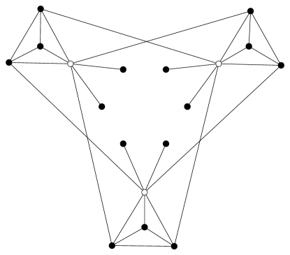
$\!\!\!\!\!\!\!\!\!\!\begin{array}[]{ccc}t^{2}-8t+8,\!\!\!\!\!\!\!\!\!\!\!\!\!\!\!\!\!\!\!\!\!\!\!\!&&\!\!\!\!\!\!\!\!\!\!\!\!\!\!\!\!\!\!\!\!\!\!\!\!t^{2}+4t-4\\ &&\\ &t-2&\\ &&\\ &t^{2}-2t+2&\\ &&\\ t^{2}-2,\!\!\!\!\!\!&&\!\!\!\!\!\!t^{2}-4t+2\\ &\\ &\\ &\\ &\\ &\\ &\\ &\\ \end{array}$

Figure 2.1. The graph $\Gamma(\{2\})^{2}$. The polynomials represented by the vertices in the lower third of the graph are indicated.

The three white vertices are the polynomials in ${\mbox{\rm Polys}}_{1}(\{2\})$ and the subgraph $\Gamma(\{2\})^{1}$ consists of three isolated points. The fifteen black vertices are the elements of ${\mbox{\rm Polys}}_{2}(\{2\})$. That the drawn graph is indeed all of $\Gamma(\{2\})^{2}$ is a special case of the completeness results cited in Section 4.

The sets ${\mbox{\rm Polys}}_{2^{b}1^{a}}(\{2\})$ can all be read off of Figure 2.1, and have sizes

(2.1) $$\begin{array}[]{r|rrl}b&a=0&a=1\\ \cline{1-3}\cr 0&1&3\\ 1&15&21\\ 2&9&9\\ 3&3&3&\!\!\!\!\!\!.\!\!\!\end{array}$$

For example, the clique formed by the four lowest vertices gives the element

$$s(t)=(t^{2}-2t+2)(t^{2}-2)(t^{2}-4t+2)(t-2)$$

of ${\mbox{\rm Polys}}_{2^{3}1}(\{2\})$. The polynomial $s(t)$ and its transforms by $S_{3}$ give the bottom right $3$ of (2.1). The graph-theoretic deductions in Sections 3-6 are conceptually no different from the visual inspection of Figure 2.1 needed to produce (2.1). However the graphs involved are much larger and the passage from graphs to cliques is incorporated into our programs as described next.

2.7. Step 3 of the process

To compute a graph $\Gamma(P)^{f}$ and all associated sets ${\mbox{\rm Polys}}_{\kappa}(P)$, the first two steps as described in §1.2 yield the vertex set ${\mbox{\rm Polys}}(P)^{f}_{1}$. Step 3, passing from the vertex set to the entire graph, is then done as follows. For each vertex $s_{1}(t)\in{\mbox{\rm Polys}}(P)^{f}_{1}$ we compute resultants and determine its set $N_{s_{1}(t)}$ of lesser neighbors with respect to some ordering. The edge set ${\mbox{\rm Polys}}(P)^{f}_{2}$ is then all $s_{1}(t)s_{2}(t)$ with $s_{2}(t)\in N_{s_{1}(t)}$. One continues inductively, with ${\mbox{\rm Polys}}(P)^{f}_{\ell}$ being the set of $s_{1}(t)\cdots s_{\ell}(t)$ with $s_{\ell}(t)\in\cap_{i=1}^{\ell-1}N_{s_{i}(t)}$.

2.8. Monic variants

If $s(t)\in{\mathbb{Z}}[t]$ is a normalized polynomial then $s(t)/s(\infty)\in{\mathbb{Q}}[x]$ is a monic polynomial. It is often technically more convenient to work with monic rather than normalized polynomials. Accordingly, we let ${\mbox{\rm MPolys}}(P)$ be the set of monic polynomials $s(t)/s(\infty)$ with $s(t)\in{\mbox{\rm Polys}}(P)$. So elements of ${\mbox{\rm MPolys}}(P)$ lie in ${\mathbb{Z}}^{P}[t]$, where ${\mathbb{Z}}^{P}$ is the ring of rational numbers with denominators in $P^{*}$. As a general rule, we keep the focus on ${\mbox{\rm Polys}}(P)$, switching temporarily to the very mild variant ${\mbox{\rm MPolys}}(P)$ only when it is truly preferable.

3. 1-split polynomials

This section describes how one determines the sets ${\mbox{\rm Polys}}_{1^{a}}(P)$, We illustrate the procedure by determining ${\mbox{\rm Polys}}_{1^{a}}(\{2,3,5,7\})$ for all $a\in{\mathbb{Z}}_{\geq 0}$.

3.1. Vertices via ABC triples

Step 1 from the introduction is trivial, since the only degree one number field is ${\mathbb{Q}}$. Step 2 is to determine the polynomials which lie in the vertex set ${\mbox{\rm Polys}}_{1}(P)$ of the graph $\Gamma(P)^{1}$. To make the $S_{3}$-symmetry of §2.5 completely evident it is convenient to work with ABC triples.

Definition 3.1.

For a rational number $u\neq 0,1$, let $A$, $B$, and $C$ be the unique pairwise relatively prime integers with $u=-A/C$, $A+B+C=0$, and $ABC<0$. For a set of primes $P$, the set $T_{\infty,\infty,\infty}({\mathbb{Z}}^{P})$ is the set of $u$ such that $A$, $B$, and $C$ are in $P^{*}$.

The notation $T_{\infty,\infty,\infty}({\mathbb{Z}}^{P})$ is a specialization of the general notation $T_{p,q,r}({\mathbb{Z}}^{P})$ of [12], and we will use other special cases in the next two sections. The action of $S_{3}$ on ABC triples by permutations corresponds to an action of $S_{3}$ on the projective $u$-line by fractional linear transformations, with $(AB)$ corresponding to $u\mapsto 1-u$ and $(AC)$ to $u\mapsto 1/u$. Using the alternative monic language of §2.8, one has

$${\mbox{\rm MPolys}}_{1}(P)=\{t-u\}_{u\in T_{\infty,\infty,\infty}({\mathbb{Z}}^{P})}.$$

This very simple parametrization is a prototype for the more complicated parametrizations given in Theorems 4.1 and 5.1.

The set $T_{\infty,\infty,\infty}({\mathbb{Z}}^{P})$ is empty if $2\not\in P$ by Reduction Bound 2.1. Otherwise $\{-1,1/2,2\}$ is a three-element $S_{3}$-orbit and all other $S_{3}$-orbits have size six. Elements of $T_{\infty,\infty,\infty}({\mathbb{Z}}^{P})$ can be found by computer searches: to get all those with $\mbox{height}(u):=\max(|A|,|C|)$ less than a certain cutoff, one searches over candidate $(A,C)$ and selects those for which $B=-A-C$ is also in $P^{*}$.

In the case $P=\{2,3,5,7\}$, a search up to height $10^{9}$ took ten seconds and yielded $375=3+6\cdot 62$ elements. The eighteen of largest height come from the ABC triples

$$(1,4374,-4375) = (1,2^{1}3^{7},-5^{4}7),$$

$$(1,2400,-2401) = (1,2^{5}3^{1}5^{2},-7^{4}),$$

$$(5,1024,-1029) = (5,2^{10},-3^{1}7^{3}).$$

All the other elements have height at most 625. The completeness of this list is a special case of a result of de Weger [17, Theorem 5.4]. This result also gives $|{\mbox{\rm Polys}}_{1}(\{2,3,5,7,11\})|=1137$ and $|{\mbox{\rm Polys}}_{1}(\{2,3,5,7,11,13\})|=3267$, with largest heights $18255$ and $1771561$ respectively.

3.2. The sets ${\mbox{\rm Polys}}_{1^{a}}({\{2,3,5,7\}})$

Tabulating cliques as described in §2.7 has a run-time of about two minutes and gives the following result.

Proposition 3.1.

The nonempty sets ${\mbox{\rm Polys}}_{1^{a}}(\{2,3,5,7\})$ have size as follows:

$${\begin{array}[]{r|rrrrrrrrrr}a&0&1&2&3&4&5&6&7&8&9\\ \hline\cr\mbox{{\rm Size}}&1&375&9900&73000&232260&383712&356916&190620&55935&7425\end{array}}$$

The sets involved in the next case $\{2,3,5,7,11\}$ are already much larger, both because of the larger vertex set and from the relaxation of the compatibility condition.

3.3. Extremal polynomials

One of the $7425$ elements of ${\mbox{\rm Polys}}_{1^{9}}(\{2,3,5,7\})$ is $s(t)=\prod_{u=2}^{10}(t-u)$. Similarly, suppose $P$ consists of all primes strictly less than a fixed prime $p$. Then $s(t)=\prod_{u=2}^{p-1}(t-u)$ realizes Reduction Bound 2.1.

The $7425$ polynomials in ${\mbox{\rm Polys}}_{1^{9}}(\{2,3,5,7\})$ are structured into packets as follows. Let $\prod_{i=1}^{9}(t-u_{i})$ be a polynomial in ${\mbox{\rm Polys}}_{1^{9}}(\{2,3,5,7\})$ and consider the twelve element set $\{u_{1},\dots,u_{9},0,1,\infty\}$. For any triple of distinct elements there is a unique fractional linear transformation in $PGL_{2}({\mathbb{Q}})$ which takes these elements in order to $0$, $1$, and $\infty$. A given element of ${\mbox{\rm Polys}}_{1^{9}}(\{2,3,5,7\})$ determines $12\cdot 11\cdot 10/|A|$ elements of ${\mbox{\rm Polys}}_{1^{9}}(\{2,3,5,7\})$ in this way, with $A$ its stabilizer subgroup. There are in fact thirteen such packets, eight with stabilizer subgroup $C_{2}$ and one each with stabilizer $C_{1}$, $V$, $S_{3}$, $D_{4}$ and $D_{6}$. The product $\prod_{u=2}^{10}(t-u)$ is in one of the eight packets with stabilizer $C_{2}$, its nontrivial automorphism being $t\mapsto 11-t$. As another example, the element

$$s(t)=(t+14)(t+8)(t+5)(t+4)(t+2)(t-2)(t-4)(t-10)(t-16)$$

represents the packet with trivial stabilizer $C_{1}$. The numbers presented are consistent via the mass-check

$$\frac{7425}{12\cdot 11\cdot 10}=5.875=1+8\cdot\frac{1}{2}+\frac{1}{4}+\frac{1}{6}+\frac{1}{8}+\frac{1}{12}.$$

The two minute run-time cited above corresponds to a simple program which does not exploit this type of symmetry.

4. 2-split polynomials

This section describes how one determines sets ${\mbox{\rm Polys}}_{2^{b}1^{a}}(P)$. Without loss of generality we restrict to $P$ containing $2$ throughout this section. Assuming ${\mbox{\rm Polys}}_{1}(P)$ as known from the previous section, to complete Steps 1 and 2 one needs to determine ${\mbox{\rm Polys}}_{2}(P)$ and Theorem 4.1 gives our method. We illustrate the full procedure by determining all ${\mbox{\rm Polys}}_{2^{b}1^{a}}(\{2,3,5\})$.

4.1. Vertices via $ABC$ triples

Let $T_{\infty,2,\infty}({\mathbb{Z}}^{P})$ be the set of rational numbers $w=-A/C$ exactly as in Definition 3.1 except that $B=-A-C$ is only required to have the form $by^{2}$ with $b\in P^{*}$. For an element $w\in T_{\infty,2,\infty}({\mathbb{Z}}^{P})$, its discriminant class by definition is $\delta=w(1-w)\in{\mathbb{Q}}^{\times}/{\mathbb{Q}}^{\times 2}$. This invariant gives a decomposition

$$T_{\infty,2,\infty}({\mathbb{Z}}^{P})=\coprod_{\delta}T_{\infty,2,\infty}({\mathbb{Z}}^{P})^{\delta}.$$

This decomposition is used in Theorem 4.1 below as one of two aspects of compatibility.

To find all $w$ in $T_{\infty,2,\infty}({\mathbb{Z}}^{P})$ up to a height bound of $H$, one searches over the exact same set of $(A,C)$ as in the search for elements of $T_{\infty,\infty,\infty}({\mathbb{Z}}^{P})$. However now one keeps those $(A,C)$ where the square-free part of $B=-A-C$ is in $P^{*}$. For our example, we need the set $T_{\infty,2,\infty}({\mathbb{Z}}^{\{2,3,5\}})$. A one-second search up to cutoff $H=10^{9}$ found $183$ elements. The list consists of $-1$ and then $92$ reciprocal pairs. The three pairs of largest height come from the triples

$$(1,-25921,25920) = (1,161^{2},2^{6}3^{4}5),$$

$$(9,-64009,64000) = (3^{2},-253^{2},2^{9}5^{3}),$$

$$(15625,-17161,1536) = (5^{6},-131^{2},2^{9}3).$$

All the other elements have height at most 6561. The completeness of this list follows from [5], where the larger set $T_{3,2,\infty}({\mathbb{Z}}^{\{2,3,5\}})$ is calculated to have 440 elements. The distribution according to discriminant class $\delta$ is quite uneven, and given after the proof of Theorem 4.1 below.

4.2. From the set $T_{\infty,2,\infty}({\mathbb{Z}}^{P})$ of $ABC$ triples to the set ${\mbox{\rm Polys}}_{2}(P)$ of degree two vertices in $\Gamma(P)$

A general quadratic polynomial in ${\mathbb{Q}}[x]$ can be written uniquely in the form

(4.1) $$s(u_{0},u_{1},u_{\infty};t)=u_{\infty}t^{2}+(u_{1}-u_{0}-u_{\infty})t+u_{0}$$

with $(u_{0},u_{1},u_{\infty})\in{\mathbb{Q}}^{3}$. Its discriminant is

$$\Delta(u_{0},u_{1},u_{\infty}) = (u_{1}-u_{0}-u_{\infty})^{2}-4u_{0}u_{\infty}$$

$$= \left(u_{0}^{2}+u_{1}^{2}+u_{\infty}^{2}\right)-2\left(u_{0}u_{1}+u_{0}u_{\infty}+u_{1}u_{\infty}\right).$$

To complete an identification of the new part ${\mbox{\rm Polys}}_{2}(P)$ of the vertex set, we use the following result, which naturally gives ${\mbox{\rm Polys}}_{[2]}(P)={\mbox{\rm Polys}}_{2}(P)\coprod{\mbox{\rm Polys}}_{1^{2}}(P)$.

Theorem 4.1.

Let $P$ be a finite set of primes containing $2$. Let $(\delta;w_{0},w_{1},w_{\infty})$ run over triples where $\delta\in P^{*}$ is a square-free integer and the $w_{i}$ are in $T_{\infty,2,\infty}({\mathbb{Z}}^{P})^{\delta}\cup\{1\}$ satisfying

(4.3) $$\Delta(w_{0},w_{1},w_{\infty})=-4w_{0}w_{1}w_{\infty}.$$

Then the polynomials

(4.4) $$S(w_{0},w_{1},w_{\infty})=\frac{1}{w_{\infty}}s(w_{0},w_{1},w_{\infty};t)$$

have discriminant class $\delta$ and run over ${\mbox{\rm MPolys}}_{[2]}(P)$

Proof.

Just using that $w_{0}$, $w_{1}$, $w_{\infty}$ are all in ${\mathbb{Z}}^{P\times}$ one immediately gets that $S(0)$, $S(1)$, $S(\infty)$ are all in ${\mathbb{Z}}^{P\times}$. Assuming further that $(w_{0},w_{1},w_{\infty})$ satisfies (4.3), then the discriminant $\Delta(w_{0},w_{1},w_{\infty})$ is also in ${\mathbb{Z}}^{P\times}$. Thus quadratic polynomials as in the theorem are indeed in ${\mbox{\rm MPolys}}_{[2]}(P)$. The issue which remains is that these polynomials form all of ${\mbox{\rm MPolys}}_{[2]}(P)$. To prove this converse direction we start with the hypothesis that $s(u_{0},u_{1},u_{\infty};t)/u_{\infty}\in{\mbox{\rm MPolys}}_{[2]}(P)$ and deduce that $(u_{0},u_{1},u_{\infty})$ is proportional to a triple $(w_{0},w_{1},w_{\infty})$ as in the theorem.

In general, suppose given an ordered triple of disjoint divisors $(D_{2},D_{1a},D_{1b})$ on the projective line ${\mathbb{P}}^{1}$ over ${\mathbb{Q}}$, of degrees $2$, $1$, and $1$ respectively. After applying a fractional linear transformation, one can partially normalize so that $D_{1a}=\{0\}$, $D_{1b}=\{\infty\}$, and $D_{2}$ consists of the roots of $t^{2}+bt+c$ with $b$, $c\in{\mathbb{Q}}$. To continue with the normalization, suppose $b\neq 0$. Then one can uniquely scale so that still $D_{1a}=\{0\}$ and $D_{1b}=\{\infty\}$ but now $D_{2}$ consists of the roots of $t^{2}-t+v$ for $v=c/b^{2}$ in ${\mathbb{Q}}$. Writing $v=1/4(1-w)$, one gets that $PGL_{2}({\mathbb{Q}})$-orbits of the initial tuple $(D_{2},D_{1a},D_{1b})$ yielding $b\neq 0$ are in bijection with $w\in{\mathbb{Q}}-\{0,1\}$. Moreover, the discriminant class in ${\mathbb{Q}}^{\times}/{\mathbb{Q}}^{\times 2}$ of the divisor $D_{2}$ is $w(1-w)$. Moreover, the orbit has a representative with good reduction outside of $P$ if and only if $w\in T_{\infty,2,\infty}({\mathbb{Z}}^{P})$. There are infinitely many different orbits yielding $b=0$ and we associate all of them to $w=1$.

Let $Z$ be the roots of (4.1). Then the invariants associated to $(Z,\{1\},\{\infty\})$, $(Z,\{\infty\},0)$, and $(Z,\{0\},\{1\})$ work out respectively to

$$(w_{0},w_{1},w_{\infty})=\frac{-\Delta(u_{0},u_{1},u_{\infty})}{4u_{0}u_{1}u_{\infty}}(u_{0},u_{1},u_{\infty}).$$

Thus any element of ${\mbox{\rm MPolys}}_{[2]}(P)$ is indeed of the special form (4.4). ∎

Let ${\mbox{\rm Polys}}^{\delta}_{[2]}(P)$ be the subset of ${\mbox{\rm Polys}}_{[2]}(P)$ consisting of polynomials of discriminant class $\delta$. Applying Theorem 4.1 for $P=\{2,3,5\}$ to the known set $T_{\infty,2,\infty}({\mathbb{Z}}^{P})$ gives sizes as follows:

$${\begin{array}[]{r|rrrrrrrrrrrrrrrr}\delta&-30&-15&-10&-6&-5&-3&-2&-1&1&2&3&5&6&10&15&30\\ \hline\cr|T_{\infty,2,\infty}({\mathbb{Z}}^{P})^{\delta}|&3&6&24&25&11&8&6&49&12&9&2&9&6&0&13&0\\ |{\mbox{\rm Polys}}^{\delta}_{[2]}({\mathbb{Z}}^{P})|&12&48&456&504&138&84&48&1020&171&108&10&96&48&0&204&0\end{array}}$$

Define the height of a normalized polynomial (4.1) to be $\max(|u_{0}|,|u_{1}|,|u_{\infty}|)$. With this definition, the height of a polynomial (4.1) depends only on its $S_{3}$ orbit. The three $S_{3}$-orbits with largest height all have height $3125=5^{5}$. They are represented by the following elements:

$$(w_{0},w_{1},w_{\infty}) =\frac{(-3^{7},2^{7},5^{5})}{5^{3}}, s(t) =3125t^{2}-810t-2187$$

$$(w_{0},w_{1},w_{\infty}) =\frac{(-3^{3},2^{11},5^{5})}{2^{5}3\!\cdot\!5}, s(t) =(25t-9)(125t+3),$$

$$(w_{0},w_{1},w_{\infty}) =\frac{(-3,2^{10}3,5^{5})}{2^{6}3^{2}5}, s(t) =(25t-1)(125t+3).$$

4.3. The sets ${\mbox{\rm Polys}}_{2^{b}1^{a}}(\{2,3,5\})$

Inductively tabulating cliques in $\Gamma(\{2,3,5\})^{2}$ gives the following statement

Proposition 4.1.

The nonempty sets ${\mbox{\rm Polys}}_{2^{b}1^{a}}(\{2,3,5\})$ have size as in Table 4.1.

The computation required to carry out Step 3 and thereby prove Proposition 4.1 took about two hours.

$$\begin{array}[]{r|rrrrrr}b&a=0&a=1&a=2&a=3&a=4&a=5\\ \hline\cr 0&1&99&1020&3100&3570&1386\\ 1&1927&18225&60240&90640&64470&18018\\ 2&44967&227751&477540&511200&279930&64176\\ 3&238255&862029&1347060&1125940&502530&99960\\ 4&551944&1567746&1913760&1269160&463470&83034\\ 5&745824&1740246&1683180&867600&246120&40698\\ 6&692476&1364910&1050150&409570&81690&12768\\ 7&480862&812520&493440&146800&20370&3360\\ 8&259974&376650&170850&38550&3990&756\\ 9&112016&138096&39660&6020&420&84\\ 10&39404&42216&5520&380&&\\ 11&11520&11436&360&&&\\ 12&2751&2709&&&&\\ 13&495&495&&&&\\ 14&57&57&&&&\\ 15&3&3&&&&\\ \end{array}$$

Table 4.1. Size of the nonempty sets ${\mbox{\rm Polys}}_{2^{b}1^{a}}(\{2,3,5\})$.

The fact that all $a$’s appearing in Table 4.1 are at most five is known by Reduction Bound 2.1, because ${\mathbb{P}}^{1}({\mathbb{F}}_{7})$ has only five elements besides $0$, $1$, and $\infty$. In contrast, ${\mathbb{P}}^{1}({\mathbb{F}}_{49})-\{0,1,\infty\}$ has $N(7,2)=47$ elements, corresponding to the bound $2b+a\leq 47$. Thus our computation identifies many ${\mbox{\rm Polys}}_{2^{b}1^{a}}(\{2,3,5\})$ as empty even though the reduction bound allows them to be non-empty.

4.4. Extremal Polynomials

One of the three elements in ${\mbox{\rm Polys}}_{2^{15}1}(\{2,3,5\})$ is

$$s(t) = \left(t^{2}+6t+3\right)\left(3t^{2}+6t+1\right)\left(t^{2}-6t+3\right)\left(3t^{2}-6t+1\right)\cdot$$

$$\left(t^{2}-2t-5\right)\left(5t^{2}+2t-1\right)\left(t^{2}+2t-5\right)\left(5t^{2}-2t-1\right)\cdot$$

$$\left(t^{2}-2t-1\right)\left(t^{2}+2t-1\right)\cdot\left(t^{2}-6t-1\right)\left(t^{2}+6t-1\right)\cdot$$

$$\left(3t^{2}-2t-3\right)\left(3t^{2}+2t-3\right)\cdot\left(t^{2}+1\right)\cdot(t+1).$$

Its discriminant is $2^{1046}3^{80}5^{104}$. Its roots, together with $1$, are visibly invariant under the four-element group generated by negation and inversion, with minimal invariant factors separated by $\cdot$’s. The other two elements of ${\mbox{\rm Polys}}_{2^{15}1}(\{2,3,5\})$ are obtained from the given one by applying the transformations $t\mapsto 1-t$ and $t\mapsto t/(t-1)$.

5. 3-split polynomials

This section describes how one determines sets ${\mbox{\rm Polys}}_{3^{c}2^{b}1^{a}}(P)$. Without loss of generality we restrict to $P$ containing $2$ and $3$ throughout this section. Assuming that ${\mbox{\rm Polys}}_{1}(P)$ and ${\mbox{\rm Polys}}_{2}(P)$ are known from the previous two sections, to complete Step 1 and 2 of the introduction, one needs to determine ${\mbox{\rm Polys}}_{3}(P)$ and Theorem 5.1 gives our method. We illustrate the full procedure by determining all ${\mbox{\rm Polys}}_{3^{c}2^{b}1^{a}}({\{2,3\}})$.

5.1. Compatible $ABC$ triples and vertices

Let $T_{3,2,\infty}({\mathbb{Z}}^{P})$ be the set of rational numbers $j=-A/C$ exactly as in Definition 3.1 except that $A$ and $B=-A-C$ are only required to have the respective forms $ax^{3}$ and $by^{2}$ with $a,b\in P^{*}$. For an element $j\in T_{3,2,\infty}({\mathbb{Z}}^{P})$ the polynomial

(5.1) $$S(j,t) = 4(j-1)t^{3}-27jt-27j$$

has discriminant $3^{9}j^{2}/2^{4}(j-1)^{3}$. Let $c$ be the isomorphism class of the algebra ${\mathbb{Q}}[t]/S(j,t)$. This invariant gives a decomposition

(5.2) $$T_{3,2,\infty}({\mathbb{Z}}^{P})=\coprod_{c}T_{3,2,\infty}({\mathbb{Z}}^{P})^{c}.$$

This decomposition is used in Theorem 5.1 below as one of two aspects of compatibility.

To find all $j$ in $T_{3,2,\infty}({\mathbb{Z}}^{P})$ up to a height bound of $H$, one searches as before over $(A,C)$. Now, however, the search is substantially larger as one only has $A=ax^{3}$ with $a\in P^{*}$. For our example, we need the set $T_{3,2,\infty}({\mathbb{Z}}^{\{2,3\}})$. A three minute search up to cutoff $10^{11}$ found 81 elements. Of these, the factorization partition of (5.1) is $3$, $21$, and $1^{3}$ respectively $54$, $24$, and $3$ times. The four $j$’s with (5.1) irreducible of largest height come from the triples

$$(-73085409,73085401,8) = (-3^{5}67^{3},8466^{2},2^{3}),$$

$$(128787625,-531440809,402653184) = (505^{3},-25053^{2},2^{27}3),$$

$$(7022735875,-7022744067,8192) = (1915^{3},3^{1}48383^{2},2^{13}),$$

$$(67867385039,-67867385042,3) = (4079^{3},-2^{1}184211^{2},3).$$

All the other elements have height at most 3,501,153. The completeness of this $81$-element list dates back to [4]; it is also a subset of the $440$-element set $T_{3,2,\infty}({\mathbb{Z}}^{\{2,3,5\}})$ from [5] cited in the previous section. The distribution of the $54$ irreducible $j$-invariants according to isomorphism class $c$ is quite uneven, and given in Table 5.1 below.

5.2. From the set $T_{3,2,\infty}({\mathbb{Z}}^{P})$ of $ABC$ triples to the set ${\mbox{\rm Polys}}_{3}(P)$ of degree three vertices in $\Gamma(P)$

The current situation is similar to the passage from $T_{\infty,2,\infty}({\mathbb{Z}}^{P})$ to ${\mbox{\rm Polys}}_{2}(P)$ but more complicated. The discriminant of a monic cubic polynomial $s(t)=t^{3}+bt^{2}+ct+d$ is

$$\Delta(b,c,d)=-4b^{3}d+b^{2}c^{2}+18bcd-4c^{3}-27d^{2}.$$

If $s(t)$ is separable, so that $\Delta(b,c,d)$ is nonzero, the $j$-invariant is then

$$j=\frac{4(b^{2}-3c)^{3}}{27\Delta(b,c,d)}.$$

If one changes $s(t)$ to $m^{-3}s(mt+b)$ the $j$-invariant does not change. One can expect $j$-invariants to play a central role in our situation because for $j\neq 0,1$, polynomials in $s(t)\in{\mathbb{Q}}[t]$ with a given $j$-invariant are all transforms of each other by fractional linear transformations in $PGL_{2}({\mathbb{Q}})$.

Let

$$F(j,k,y) = k\left(j^{2}y^{3}-2jy^{3}+3jy^{2}-3jy+1\right)^{2}-j\left(jy^{2}-2y+1\right)^{3}$$

$$= j^{2}\left(j^{2}k-j^{2}-4jk+4k\right)y^{6}+\mbox{(terms of lower order in $y$)}.$$

We say that $\infty$ is a root of $F(j,k,y)$ if the coefficient of $y^{6}$ is zero. This polynomial is important for us because for $j,k\in{\mathbb{Q}}-\{0,1\}$, roots of $F(j,k)$ in $\overline{{\mathbb{Q}}}\cup\{\infty\}$ are in natural $\mbox{Gal}(\overline{{\mathbb{Q}}}/{\mathbb{Q}})$-equivariant bijection with bijections from roots of $S(j,t)$ to roots of $S(k,t)$. Note that

$$\mbox{disc}_{y}(F(j,k,y))=2^{22}3^{6}j^{10}(j-1)^{15}k^{4}(k-1)^{3}.$$

Thus there indeed always six roots when $j,k\in{\mathbb{Q}}-\{0,1\}$.

Theorem 5.1.

Let $P$ be a finite set of primes containing $2$ and $3$. Let $c$ be the isomorphism class of a cubic field in $NF_{3}(P)$ and let $j\in T_{3,2,\infty}({\mathbb{Z}}^{P})^{c}$. The polynomials in ${\mbox{\rm MPolys}}_{3}(P)^{c}$ with $j$-invariant $j$ are among the polynomials

$$s^{m,n}_{j_{0},j_{1},j}(t) = \frac{(j-1)(t(n-m)-n)^{3}+(j-1)jm^{3}n^{3}-j(mn-mt+nt-n)^{3}}{(m-n)^{3}}$$

with $j_{0}$, $j_{1}\in(T_{3,2,\infty}({\mathbb{Z}}^{P}))^{c}\cup\{0\}$. Here $m$ and $n$ run over solutions in ${\mathbb{Q}}\cup\{\infty\}$ of $F(j,j_{0},y)=0$ and $F(j,j_{1},y)=0$ respectively.

If $m$ and/or $n$ is $\infty$, one needs to understand the definition of $s^{m,n}_{j_{0},j_{1},j}(t)$ in a limiting sense. For example, $s_{j_{0},j_{1},j}^{\infty,n}(t)=t^{3}-3jnt^{2}+3jn^{2}t+j(j-2)n^{3}$

Proof.

Let $s(t)=s_{\infty}(t)=t^{3}+bt^{2}+ct+d$ be a polynomial in ${\mbox{\rm MPolys}}_{3}(P)^{c}$. Then one has not only its usual $j$-invariant $j$, but also the $j$-invariants $j_{0}$ and $j_{1}$ of the transformed polynomials

$$s_{0}(t)=\frac{t^{3}}{d}s\left(\frac{1}{t}\right)\mbox{ and }s_{1}(t)=\frac{(t-1)^{3}}{1+b+c+d}s\left(\frac{t}{t-1}\right).$$

These two new $j$-invariants lie in $(T_{3,2,\infty}({\mathbb{Z}}^{P}))^{c}\cup\{0\}$, with $0$ only possible only if $\mbox{disc}(s)$ is $-3$ times a square.

Recovering all possibilities for $s(t)$ from the three invariants $(j_{0},j_{1},j)$ is complicated, because thirty-six different polynomials $x^{3}+bx^{2}+cx+d\in\overline{{\mathbb{Q}}}[x]$ give rise to a given generic $(j_{0},j_{1},j)\in\overline{{\mathbb{Q}}}^{3}$. Note that

$$\mbox{disc}_{t}(s^{m,n}_{j_{0},j_{1},j}(t))=\frac{2^{2}3^{3}j^{2}(j-1)^{2}m^{6}n^{6}}{(m-n)^{6}}.$$

For generic $(j_{0},j_{1},j)$ the thirty-six polynomials are just the thirty-six $s_{j_{0},j_{1},j}^{m,n}(t)$ as $(m,n)$ varies over solutions to $F(j,j_{0},m)=F(j,j_{1},n)=0$. The coordinate relations

(5.3) $$m = -\frac{9\Delta(b,c,d)}{2\left(b^{2}-3c\right)\left(b^{2}c+9bd-6c^{2}\right)},$$

(5.4) $$n = -\frac{9\Delta(b,c,d)}{2\left(b^{2}-3c\right)\left(2b^{3}+b^{2}c-9bc+9bd-6c^{2}+27d\right)}$$

let one verify this statement algebraically.

There remains the concern that for nongeneric $(j_{0},j_{1},j)$, there may be cubics in ${\mbox{\rm MPolys}}_{3}(P)^{c}$ which are not among the $s_{j_{0},j_{1},j}^{m,n}(t)$. This indeed happens in the excluded case $j=0$, as discussed just after this proof. The case $j=1$ is not relevant for the theorem because $S(1,t)=-27(1+t)$ is not an irreducible cubic. The cases $m=0$, $n=0$, and $m=n$ arise only when $j=j_{0}$, $j=j_{1}$, and $j_{0}=j_{1}$. Corresponding polynomials in ${\mbox{\rm MPolys}}_{3}(P)^{c}$ would have to be stable under $t\mapsto 1/t$, $t\mapsto t/(t-1)$, or $t\mapsto 1-t$ respectively. But there are no such stable polynomials because the commutator of the possible Galois groups $A_{3}$ and $S_{3}$ in $S_{3}$ does not contain an element of order two. Thus, despite the occasional inseparability of $s^{m,n}_{j_{0},j_{1},j}(t)$, all polynomials in ${\mbox{\rm MPolys}}_{3}(P)^{c}$ with nonzero $j$-invariant are indeed among the $s^{m,n}_{j_{0},j_{1},j}(t)$. ∎

To get the complete determination of ${\mbox{\rm MPolys}}_{3}(P)$ we need to complement the polynomials coming directly from Theorem 5.1 with the list of polynomials with $j=0$. A calculation shows that there are no separable polynomials at all with $(j_{0},j_{1},j)=(0,0,0)$. So if $j$ is zero, at least one of $j_{0}$ and $j_{1}$ is nonzero. So the remaining polynomials are in fact just $S_{3}$-translates of polynomials already found.

Some further comments clarify Theorem 5.1 and how it is used in the construction of ${\mbox{\rm MPolys}}_{3}(P)$. Since $j\neq 0$ and the $j_{i}$ belong to the same cubic field, there is a common Galois group, $G\in\{A_{3},S_{3}\}$. The polynomials $F(j,j_{i},y)$ can factor into irreducibles in three different ways:

$$F(j,j_{i},y)=\left\{\begin{array}[]{ll}(\mbox{cubic})(\mbox{quadratic})(\mbox{linear})&\mbox{($G=S_{3}$, $j_{i}\neq 0$),}\\ (\mbox{cubic})(\mbox{linear})(\mbox{linear})(\mbox{linear})&\mbox{($G=A_{3}$),}\\ -(s^{2}-1)^{4}(y-\frac{1}{1-s})^{3}(y-\frac{1}{1+s})^{3}&\mbox{($G=S_{3}$, $j_{i}=0$, $j=1-s^{2}$).}\end{array}\right.$$

In the $A_{3}$ case, always $3^{2}=9$ of the thirty-six $s_{j_{0},j_{1},j}^{m,n}(t)$ are in ${\mathbb{Q}}[x]$. In the $S_{3}$ case with $w$ zeros among $\{j_{0},j_{1}\}$ there are $2^{w}$ rational polynomials. Of course it is trivial to see whether a candidate $s_{j_{0},j_{1},j}^{m,n}(t)$ from the theorem is actually in ${\mbox{\rm MPolys}}_{3}(P)$. Namely, if $m$ and $n$ are both finite then the quantities

$$s^{m,n}_{j_{0},j_{1},j_{\infty}}(0) = \frac{n^{3}\left(j^{2}m^{3}-2jm^{3}+3jm^{2}-3jm+1\right)}{(m-n)^{3}},$$

$$s^{m,n}_{j_{0},j_{1},j_{\infty}}(1) = \frac{m^{3}\left(j^{2}n^{3}-2jn^{3}+3jn^{2}-3jn+1\right)}{(m-n)^{3}},$$

$$\mbox{disc}_{t}(s_{j_{0},j_{1},j_{\infty}}^{m,n}(t)) = \frac{108(j-1)^{3}j^{2}m^{6}n^{6}}{(m-n)^{6}}$$

need to all be in ${\mathbb{Z}}^{P\times}$. When $m$ and/or $n$ is $\infty$, one just uses the limiting forms of these expressions.

Table 5.1 summarizes the determination of ${\mbox{\rm Polys}}_{3}(\{2,3\})$.

$$\begin{array}[]{rrl c r c | llrcr}\lx@intercol\hfil d\hfil\lx@intercol&\lx@intercol\hfil D\hfil\lx@intercol&\lx@intercol\hfil f(t)\hfil\lx@intercol&\lx@intercol\hfil T_{3,2,\infty}({\mathbb{Z}}^{\{2,3\}})^{c}\hfil\lx@intercol\vrule\lx@intercol&\lx@intercol\hfil|{\mbox{\rm Polys}}_{3}(\{2,3\})^{c}|\hfil\lx@intercol\\ \hline\cr-6&-216&t^{3}+3t-2&&10&&6(66)&&&=&396\\ -3&-972&t^{3}-12&&1&&6(&&1)&=&6\\ -3&-972&t^{3}-6&&1&&6(&&1)&=&6\\ -3&-243&t^{3}-3&&6&&6(13&+13&+4)&=&180\\ -3&-108&t^{3}-2&&4&&6(4&+9&+3)&=&96\\ -2&-648&t^{3}-3t-10&&9&&6(17)&&&=&102\\ -1&-324&t^{3}-3t-4&&9&&6(44)&&&=&264\\ 1&81&t^{3}-3t-1&&3&&6(6&+10)&+2(2)&=&100\\ 6&1944&t^{3}-9t-6&&11&&6(58)&&&=&348\\ \cline{5-5}\cr\cline{11-11}\cr&&&&54&&&&&&1498\end{array}$$

Table 5.1. The nine cubic fields ${\mathbb{Q}}[t]/f(t)$ with discriminant $\pm 2^{a}3^{b}$ and associated integers.

The last block of columns illustrates how a general decomposition of ${\mbox{\rm Polys}}_{3}(P)^{c}$ into $S_{3}$-orbits appears in the case $P=\{2,3\}$. Let $d$ be the square-free integer agreeing with the field discriminant $D$ modulo squares. If $d\neq 1$ then all orbits have size six. Orbits are usually indexed by triples of distinct $j$-invariants. However for $d=-3$, an unordered triple $(j_{0},j_{1},0)$ can index up to two orbits and an unordered triple $(0,0,j)$ can index up to one orbit. The contributions from each possibility in the case $P=\{2,3\}$ are listed in order. For $d=1$, an unordered triple $(j_{0},j_{1},j_{\infty})$ can index up to $9$, $6$, or $1$ orbits, depending on whether it contains $3$, $2$, or $1$ distinct $j$-invariants. All orbits again have size six, except for the ones indexed by $(j,j,j)$, which have size two. The contributions from each possibility in the case $P=\{2,3\}$ are again listed in order.

$$\begin{array}[]{rr|rrrrrrrr}c&a&b=0&b=1&b=2&b=3&b=4&b=5&b=6&b=7\\ \hline\cr 0&0&1&169&981&1723&1390&630&150&12\\ 0&1&21&675&2175&2559&1416&486&108&12\\ 0&2&60&840&1710&1200&270&&&\\ 0&3&40&340&570&340&70&&&\\ \hline\cr 1&0&1498&6364&10854&8788&3958&1116&162&\\ 1&1&4584&13632&18024&11280&3600&792&96&\\ 1&2&4260&9900&10020&4800&720&&&\\ 1&3&1120&2440&2040&1000&160&&&\\ \hline\cr 2&0&21282&37374&34008&16866&4560&798&72&\\ 2&1&41184&62208&49872&21000&3900&564&48&\\ 2&2&24720&33180&23160&8940&900&&&\\ 2&3&3960&6000&3720&1680&240&&&\\ \hline\cr 3&0&81850&95578&54942&17398&2704&216&&\\ 3&1&117288&133632&71712&19800&1992&120&&\\ 3&2&49140&54660&27240&7380&540&&&\\ 3&3&4520&6200&2760&1000&160&&&\\ \hline\cr 4&0&156924&144000&55692&11434&1132&48&&\\ 4&1&180822&174564&64074&11004&684&24&&\\ 4&2&56910&56940&19050&2760&120&&&\\ 4&3&3030&4020&1230&220&40&&&\\ \hline\cr 5&0&173110&137530&38094&4848&282&&&\\ 5&1&167448&144552&39048&3936&144&&&\\ 5&2&42000&37260&8880&420&&&&\\ 5&3&1240&1600&360&&&&&\\ \hline\cr 6&0&116552&85214&18186&1392&42&&&\\ 6&1&95388&76440&16572&1044&24&&&\\ 6&2&19800&15360&2820&&&&&\\ 6&3&560&620&60&&&&&\\ \hline\cr 7&0&49364&33650&5622&246&&&&\\ 7&1&33576&25440&4392&192&&&&\\ 7&2&5820&4140&600&&&&&\\ 7&3&160&160&&&&&&\\ \hline\cr 8&0&12998&7916&954&24&&&&\\ 8&1&6870&4914&534&18&&&&\\ 8&2&960&720&60&&&&&\\ 8&3&20&20&&&&&&\\ \hline\cr 9&0&1948&952&54&&&&&\\ 9&1&648&456&&&&&&\\ 9&2&60&60&&&&&&\\ \hline\cr 10&0&162&54&&&&&&\\ 10&1&24&24&&&&&&\\ \hline\cr 11&0&8&2&&&&&&\\ \end{array}$$

Table 5.2. Size of the nonempty sets ${\mbox{\rm Polys}}_{3^{c}2^{b}1^{a}}({\{2,3\}})$

As an example of the complications associated to $d=-3$, let $c$ be the isomorphism class of ${\mathbb{Q}}[t]/(t^{3}-12)$. Then $T_{3,2,\infty}({\mathbb{Z}}^{\{2,3\}})^{c}=\{-24\}$. Consider $(j_{0},j_{1},j)=(0,0,-24).$ Theorem 5.1 formally yields four candidates.

$$\begin{array}[]{c|cc}m\setminus n&-1/4&1/6\\ \hline\cr-1/4&[1]&t^{3}+6t^{2}-6t+2\\ 1/6&t^{3}-9t^{2}+9t-3&[1]\\ \end{array}$$

As always for $(0,0,j)$, only the two candidates coming from $m\neq n$ are separable and these are $S_{3}$-transforms of one another. In this case, both are in ${\mbox{\rm Polys}}_{3}(\{2,3\})^{c}$. The remaining $S_{3}$-transforms are $2t^{3}-3$, $2t^{3}-6t^{2}+6t+1$, $3t^{3}-2$, and $3t^{3}-9t^{2}+9t-1$, accounting for all of ${\mbox{\rm Polys}}_{3}(\{2,3\})^{c}$.

As an example of complications associated to $d=1$, let $c$ come from $A_{3}$ field ${\mathbb{Q}}[t]/(t^{3}-t-1)$. Then $T_{3,2,\infty}({\mathbb{Z}}^{\{2,3\}})^{c}=\{1372/3,4,4/3\}$. The ordered tuple $(j_{0},j_{1},j)=(1372/3,4,4/3)$ gives nine candidates. They are

$${{\begin{array}[]{c|ccc}m\setminus n&1&1/2&\infty\\ \hline\cr 3&8t^{3}-36t^{2}+30t+1&[125t^{3}-225t^{2}+75t+1]&t^{3}+9t^{2}+15t-1\\ 3/8&[125t^{3}-300t^{2}+180t-8]&t^{3}-6t^{2}+9t-1&64t^{3}-96t^{2}+36t-1\\ 9/10&t^{3}+6t^{2}-96t+8&64t^{3}-48t^{2}-96t-1&[125t^{3}+75t^{2}-120t+1]\end{array}}}$$

The three in brackets are rejected and the other six are members of ${\mbox{\rm Polys}}_{3}(\{2,3\})^{c}$.

5.3. The sets ${\mbox{\rm Polys}}_{3^{c}2^{b}1^{a}}(\{2,3\})$

Inductively tabulating cliques in the graph $\Gamma(\{2,3\})^{3}$ takes about 15 minutes and yields the following statement.

Proposition 5.1.

The nonempty sets ${\mbox{\rm Polys}}_{3^{c}2^{b}1^{a}}(\{2,3\})$ have size as in Table 5.2.

The largest $a$ in Table 5.2 being $3$ agrees with Reduction Bound 2.1, as there are only $3$ points in ${\mathbb{P}}^{1}({\mathbb{F}}_{5})$ beyond those already used by $\{0,1,\infty\}$.

5.4. Extreme polynomials

One of the two polynomials in ${\mbox{\rm Polys}}_{3^{11}1}(\{2,3\})$ has already been given in (1.1). It is stable under the group $A_{3}$ of even permutations of the cusps $\{0,1,\infty\}$. The minimal $A_{3}$-stable factors are given between adjacent $\cdot$’s in (1.1).

6. $f$-split polynomials with $f\geq 4$

In the previous two sections we have used $w$-invariants in $T_{\infty,2,\infty}({\mathbb{Z}}^{P})$ to construct sets ${\mbox{\rm Polys}}_{2}(P)$ and $j$-invariants in $T_{3,2,\infty}({\mathbb{Z}}^{P})$ to construct sets ${\mbox{\rm Polys}}_{3}(P)$. For degrees $d\geq 4$, we follow the three-step approach of §1.2 to determining ${\mbox{\rm Polys}}_{d}(P)$.

6.1. Excellent $P$-units and ${\mbox{\rm Polys}}_{d}(P)$

Let $K_{1}$,…, $K_{m}$ be a list of degree $d$ number fields unramified outside $P$ such that every isomorphism class of such fields appears once. Let $U_{i}$ be the $P$-unit group of $K_{i}$. The finitely generated group $U_{i}$ is well-understood and there are algorithms to produce generators. A $P$-unit $u$ is called an exceptional $P$-unit if $1-u$ is also a unit. Exceptional $P$-units have been the subject of many studies, e.g. [11].

Let $s_{u}(t)$ be the characteristic polynomial of a $P$-unit $u$. So $s_{u}(t)$ is a monic polynomial of degree $d$ in ${\mathbb{Z}}^{P}[t]$ with constant term $s_{u}(0)$ in ${\mathbb{Z}}^{P\times}$. The unit $u$ is exceptional if and only if also $s_{u}(1)\in{\mathbb{Z}}^{P\times}$. We say it is an excellent $P$-unit if furthermore $\mbox{disc}(s_{u}(t))\in{\mathbb{Z}}^{P\times}$. All elements of ${\mbox{\rm MPolys}}_{d}(P)$ arise in this way as characteristic polynomials of excellent units.

As the example of this section, we take $P=\{2\}$. The relevant set $NF_{d}(\{2\})$ of number fields is known in degrees $d\leq 15$ [6, 7]. In fact, for $d=1$, $2$, $4$, $8$ one has $|NF_{d}(\{2\})|=1$, $3$, $7$, $36$ and otherwise $NF_{d}(\{2\})=0$. The fields in question are all totally ramified at $2$. This implies that an $S_{3}$-orbit of polynomials in ${\mbox{\rm Polys}}_{d}(\{2\})$ takes one of the following forms. First, the orbit may contain just three polynomials, one of which is palindromic. In this case the palindromic polynomial $s(t)$ is the unique member of the orbit with $2|s(1)$. Second, the orbit may contain six polynomials, none palindromic. In this case, exactly two of the polynomials $s_{i}(t)$ satisfy $2|s_{i}(1)$. They are related by $t^{d}s_{1}(1/t)=\pm s_{2}(t)$.

$$\begin{array}[]{| lrlllcrrccc |}\hline\cr G&d&\lambda_{\infty}&\lambda_{3}&s(t)&\mbox{Pal}&s(1)&c&N_{1}&N_{2}&N_{4}\\ \hline\cr\lx@intercol\hfil\hfil\lx@intercol\\ \hline\cr C_{1}&1&1&1&t+1&\bullet&2&1&0&7&36\\ \hline\cr\lx@intercol\hfil\hfil\lx@intercol\\ \hline\cr C_{2}&8&11&2&t^{2}+6t+1&\bullet&8&2&1&0&7\\ &&&&t^{2}-6t+1&\bullet&-4&2&1&0&7\\ &&&&t^{2}-2t-1&&-2&1&2&2&13\\ \hline\cr C_{2}&-4&2&2&t^{2}+1&\bullet&2&1&1&2&14\\ \hline\cr C_{2}&-8&2&11&&&&&&&\\ \hline\cr\lx@intercol\hfil\hfil\lx@intercol\\ \hline\cr V&256&2&22&t^{4}+1&\bullet&2&1&1&1&4\\ &&&&t^{4}+6t^{2}+1&&8&8&1&1&2\\ \hline\cr C_{4}&2048&1111&4&t^{4}-4t^{3}-26t^{2}-4t+1&\bullet&-32&64&1&2&2\\ &&&&t^{4}+4t^{3}-26t^{2}+4t+1&\bullet&-16&64&1&2&2\\ &&&&t^{4}+28t^{3}+70t^{2}+28t+1&\bullet&128&512&1&1&0\\ &&&&t^{4}-28t^{3}+70t^{2}-28t+1&\bullet&16&512&1&1&0\\ &&&&t^{4}-4t^{3}-6t^{2}+4t+1&&-4&8&1&3&3\\ &&&&t^{4}-4t^{3}-2t^{2}+12t+1&&8&8&2&1&4\\ &&&&t^{4}+4t^{3}-2t^{2}-12t+1&&8&8&1&1&4\\ &&&&t^{4}-4t^{3}-2t^{2}+4t-1&&-2&1&2&2&7\\ &&&&t^{4}+4t^{3}-2t^{2}-4t-1&&-2&1&1&1&5\\ &&&&t^{4}-148t^{3}+102t^{2}-20t+1&&-64&512&0&0&1\\ &&&&t^{4}-20t^{3}+34t^{2}-12t+1&&4&32&0&2&0\\ \hline\cr C_{4}&2048&22&4&&&&&&&\\ \hline\cr D_{4}&-2048&211&22&t^{4}+12t^{3}+6t^{2}+12t+1&\bullet&32&64&1&2&2\\ &&&&t^{4}-12t^{3}+6t^{2}-12t+1&\bullet&-16&64&1&2&2\\ &&&&t^{4}-4t^{3}+6t^{2}-4t-1&&-2&1&1&2&5\\ \hline\cr D_{4}&-2048&211&4&t^{4}-4t^{3}-2t^{2}-4t+1&\bullet&-8&8&1&2&6\\ &&&&t^{4}+4t^{3}-2t^{2}+4t+1&\bullet&8&8&1&2&6\\ &&&&t^{4}+20t^{3}-26t^{2}+20t+1&\bullet&16&512&1&1&0\\ &&&&t^{4}-20t^{3}-26t^{2}-20t+1&\bullet&-64&512&1&1&2\\ &&&&t^{4}-2t^{2}-1&&-2&1&1&2&8\\ &&&&t^{4}-12t^{3}+10t^{2}-4t+1&&-4&8&1&2&2\\ \hline\cr D_{4}&2048&22&211&&&&&&&\\ \hline\cr D_{4}&512&22&4&t^{4}-4t^{3}+22t^{2}-4t+1&\bullet&16&64&1&1&2\\ &&&&t^{4}+4t^{3}+22t^{2}+4t+1&\bullet&32&64&1&1&2\\ &&&&t^{4}+4t^{2}-4t+1&&2&1&1&1&4\\ \hline\cr\end{array}$$

Table 6.1. Information on the sets ${\mbox{\rm Polys}}_{d}(\{2\})$ for $d\in\{1,2,4\}$

Table 6.1 describes the sets ${\mbox{\rm Polys}}_{d}({\{2\}})$ for $d\in\{1,2,4\}$ by listing polynomials representing $S_{3}$-orbits. The fields defined by $t^{2}+2$, $t^{4}+4t^{2}+2$, and $t^{4}+2$ yield no polynomials at all. Their $3$-adic factorization partitions $\lambda_{3}$ are respectively $1^{2}$, $4$, and $21^{2}$. Thus, in the case of $t^{2}+2$ and $t^{4}+2$, the nonexistence of polynomials follows from Reduction Bound 2.1. The column $\lambda_{\infty}$ gives the splitting over ${\mathbb{R}}$. The rank of $U_{i}$ is the number of parts of $\lambda_{\infty}$, and, as expected, more parts are correlated with more polynomials. Palindromic polynomials contributing three and nonpalindromic polynomials contributing six, one gets $|{\mbox{\rm Polys}}_{1}(\{2\})|=3$, $|{\mbox{\rm Polys}}_{2}(\{2\})|=15$, and $|{\mbox{\rm Polys}}_{4}(\{2\})|\geq 108$. We have taken the computation far enough that it seems unlikely that ${\mbox{\rm Polys}}_{4}(\{2\})$ contains polynomials beyond those we have found. The polynomial discriminants are $Dc^{2}$, and the largest magnitude $2^{29}$ arises in five orbits.

6.2. The sets ${\mbox{\rm Polys}}_{4^{d}2^{b}1^{a}}(\{2\})$

The last three columns of Table 6.1 indicate the nature of the known part of the graph $\Gamma(\{2\})^{4}=\Gamma(\{2\})^{7}$. For each polynomial, the number of neighbors of a given degree $d$ is given as $N_{d}$. As one would expect in general, the number of neighbors tends to decrease as the largest coefficient of the polynomial increases. Carrying out Step 3 as in §2.7 takes less than a second and yields the following result.

Proposition 6.1.

The sets ${\mbox{\rm Polys}}_{4^{d}2^{b}1^{a}}(\{2\})$ are at least as large as indicated in Table 6.2, with equality if $|{\mbox{\rm Polys}}_{4}(\{2\})|=108$.

$$\begin{array}[]{l|rrrrr}\lx@intercol\hfil|{\mbox{\rm Polys}}_{4^{d}2^{b}}(\{2\})|\hfil\lx@intercol\\ b&d:\;0&1&2&3&4\\ \hline\cr 0&1&108&177&144&42\\ 1&15&162&93&30&\\ 2&9&30&21&6&\\ 3&3&6&3&&\\ \end{array}\;\;\;\;\;\;\;\;\;\;\;\;\begin{array}[]{l|rrrrr}\lx@intercol\hfil|{\mbox{\rm Polys}}_{4^{d}2^{b}1}(\{2\})|\hfil\lx@intercol\\ b&d:\;0&1&2&3&4\\ \hline\cr 0&3&108&129&90&24\\ 1&21&156&63&18&\\ 2&9&18&9&&\\ 3&3&6&3&&\end{array}$$

Table 6.2. Size of the nonempty sets ${\mbox{\rm Polys}}_{4^{d}2^{b}1^{a}}(\{2\})$, assuming $|{\mbox{\rm Polys}}_{4}(\{2\})|=108$.

6.3. Extremal polynomials

As an extreme example, the palindromic polynomial

$$s(t) = (t+1)\left(t^{2}+1\right)\left(t^{2}-2t-1\right)\left(t^{2}+2t-1\right)$$

$$\qquad\left(t^{4}-4t^{3}-6t^{2}+4t+1\right)\left(t^{4}+4t^{3}-6t^{2}-4t+1\right)$$

has discriminant is $-2^{184}$. Its $S_{3}$ orbit in ${\mbox{\rm Polys}}_{4^{2}2^{3}1}(\{2\})$ corresponds to the bottom right $3$ in Table 6.2.

7. Large degree polynomials

In this section, we enter the third regime of §1.2: the systematic construction of polynomials in ${\mbox{\rm Polys}}_{\kappa}(P)$ in settings where complete determination of ${\mbox{\rm Polys}}_{\kappa}(P)$ is well out of reach. Each subsection focuses on degree $k$ polynomials, without pursuing details about their factorization, thus on the sets ${\mbox{\rm Polys}}_{[k]}(P)=\coprod_{\kappa\vdash k}{\mbox{\rm Polys}}_{\kappa}(P)$.

7.1. Cyclotomic polynomials

The following simple result supports the main conjecture of [16].

Proposition 7.1.

Let $P$ be a finite set of primes containing $2$ and at least one odd prime. Let ${\mbox{\rm Polys}}_{[k]}^{\rm cyclo}(P)$ be the subset of ${\mbox{\rm Polys}}_{[k]}(P)$ consisting of products of cyclotomic polynomials. Then $\lim_{k\rightarrow\infty}|{\mbox{\rm Polys}}_{[k]}^{\rm cyclo}(P)|=\infty$.

Proof.

Let $P^{\star}$ denotes the set of all integers greater than one which are divisible only by primes of $P$. For $i\in P^{\star}$, let $\Phi_{i}(t)$ be the corresponding cyclotomic polynomial, of degree $\phi(i)$. Then

(7.1) $$\sum_{k=0}^{\infty}|{\mbox{\rm Polys}}_{[k]}^{\rm cyclo}(P)|x^{k}=\prod_{i\in P^{\star}}(1+x^{\phi(i)}).$$

To treat the sets $P$ appearing in the proposition, we first consider the case $P=\{2\}$. One has $\{2\}^{\star}=\{2,4,\dots,2^{j},\dots\}$ and $\phi(2^{j})=2^{j-1}$. Expanding the product $(1+x)(1+x^{2})(1+x^{4})\cdots$, Equation (7.1) becomes

(7.2) $$\sum_{k=0}^{\infty}|{\mbox{\rm Polys}}_{[k]}^{\rm cyclo}(\{2\})|x^{k}=1+x+x^{2}+x^{3}+\cdots$$

For $P$ as in the theorem, $\sum|{\mbox{\rm Polys}}_{[k]}^{\rm cyclo}(P)|x^{k}$ is an infinite sum of $x^{j}f(x)$ with $f(x)$ as in (7.2). Thus in fact $|{\mbox{\rm Polys}}_{[k]}^{\rm cyclo}(P)|$ grows monotonically to $\infty$. ∎

A numerical example of particular relevance to Hurwitz number fields is $P=\{2,3,5\}$. Then

$$\sum_{\rho=0}^{\infty}|{\mbox{\rm Polys}}^{\rm cyclo}_{[k]}(\{2,3,5\})|x^{k}$$

$$= (1+x)(1+x^{2})^{3}(1+x^{4})^{4}(1+x^{6})^{2}\cdots$$

$$= 1+x+3x^{2}+3x^{3}+7x^{4}+\cdots+3361607445659519x^{1000}+\cdots$$

We will return to this generating function in §8.8.

7.2. Fractal polynomials

A recursive three-point cover is a rational function $F(t)\in{\mathbb{Q}}(t)$ with all critical values in $\{0,1,\infty\}$ and $F(\{0,1,\infty\})\subseteq\{0,1,\infty\}$. It has bad reduction within $P$ if one can write $F(t)=uf(t)/g(t)$ with $f(t)$ and $g(t)$ compatible polynomials in ${\mbox{\rm Polys}}(P)$ and $u\in{\mathbb{Z}}^{P\times}$. Recursive three-point covers with bad reduction within $P$ are closed under composition.

The degree $1$ recursive three-point covers form the group $S_{3}=\langle 1-t,1/t\rangle$ and have bad reduction set $P=\{\}$. Other simple examples are $F(t)=t^{p}$ for a prime $p$ with bad reduction set $\{p\}$. Combining just these via composition one already has a large collection of recursive three-point covers with solvable monodromy group [13]. One can easily extract many other recursive three-point covers from the literature. As an example coming from trinomials, $F_{m}(t)=t^{m}/(mt+1-m)$ has monodromy group $S_{m}$ and bad reduction exactly at the primes dividing $m(m-1)$. From the definitions, one has the following fact:

Pullback Construction 7.1.

Let $F(t)=uf(t)/g(t)$ be a recursive three-point cover of degree $m$ and bad reduction within $P$. Let $s(t)\in{\mbox{\rm Polys}}_{[k]}(P)$. Then the pullback $s(F(t))g(t)^{k}$ is a scalar multiple of a polynomial in ${\mbox{\rm Polys}}_{[mk]}(P)$.

We use the word “fractal” because when one constructs polynomials by iterative pullback, their roots tend to have a fractal appearance, as in Figure 7.1.

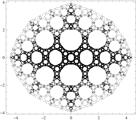
Figure 7.1. The set $R_{8,1}$ consisting of the $2^{15}=32768$ roots of the specialization polynomial $s_{8,1}(t)$ with bad reduction only at $2$.

To explain the source of Figure 7.1, and also as an example of using the pullback construction iteratively, we prove the following complement to Proposition 7.1.

Proposition 7.2.

The sets ${\mbox{\rm Polys}}_{[k]}(\{2\})$ can be arbitrarily large.

Proof.

Consider quartic recursive three-point cover

$$F(t)=\frac{-(t-1)^{2}(t+1)^{2}}{4t^{2}}=\frac{-(t^{2}+1)^{2}}{4t^{2}}+1=-\frac{\left(t^{2}-2t-1\right)\left(t^{2}+2t-1\right)}{4t^{2}}-1.$$

Its bad reduction set is $\{2\}$. Some preimages are as follows, with Galois orbits separated by semi-colons:

$$F^{-1}(0) =\{-1;\;1\}, F^{-1}(1) =\{i,-i\},$$

$$F^{-1}(\infty) =\{0;\;\infty\}, F^{-1}(-1) =\{-1-\sqrt{2},-1+\sqrt{2};\;1-\sqrt{2},1+\sqrt{2}\}.$$

Let

$$R_{1,-1} =\{-1\pm\sqrt{2}\}, R_{1,0} =\{\pm i\}, R_{1,1} =\{1\pm\sqrt{2}\}, \mbox{and }R_{i,j} =F^{1-i}(R_{1,j}).$$

The situation is summarized by the following diagrammatic description of the action of $F$ on the entire iterated preimage of $\infty$:

$$\begin{array}[]{ccccc}\vdots&&\vdots&&\vdots\\ \downarrow&&\downarrow&&\downarrow\\ R_{2,1}&&R_{2,-1}&&R_{2,0}\\ \downarrow&&\downarrow&&\downarrow\\ \!\!\!\{1\pm\sqrt{2}\}\!\!\!&&\!\!\!\{-1\pm\sqrt{2}\}\!\!\!&&\{\pm i\}\\ &\!\!\!\searrow\;\;\swarrow\!\!\!&&&\downarrow\\ &\{-1\}&&&\{1\}\\ &&\!\!\!\!\!\!\!\!\!\searrow&\swarrow\!\!&\\ &&\lx@intercol\hfil\{0\}\hfil\lx@intercol&\\ &&\lx@intercol\hfil\downarrow\hfil\lx@intercol&\\ &&\lx@intercol\hfil\{\infty\}\hfil\lx@intercol&\\ &&\lx@intercol\hfil\circlearrowleft\hfil\lx@intercol&\end{array}$$

Note that the critical values $0$, $1$, and $\infty$ have two preimages each while all other values have four preimages.

For $i\in{\mathbb{Z}}_{\geq 1}$ and $j\in\{-1,0,1\}$, let $s_{i,j}(t)\in{\mbox{\rm Polys}}_{[2^{2i-1}]}(\{2\})$ be the polynomial with roots $R_{i,j}$. Products of the form $s_{1,j_{1}}(t)\cdots s_{w,j_{w}}(t)$ give $3^{w}$ distinct polynomials in ${\mbox{\rm Polys}}_{[k]}({2})$ of the same degree $k=2(4^{w}-1)/3$. ∎

8. Specialization sets and number field construction

In this section, we sketch how the sets ${\mbox{\rm Polys}}_{\kappa}(P)$ are useful in constructing interesting number fields, focusing on two representative families of examples.

8.1. Sets $U_{\nu}(R)$

Let $\nu=(\nu_{1},\dots,\nu_{r})$ be a list of positive integers. In this section, we assume $\nu_{r-2}=\nu_{r-1}=\nu_{r}=1$ and these indices play a completely passive role. In the next section, we remove this assumption and the last three indices then take on an active role on the same footing with the other indices. Without loss of generality, we generally focus on the case where the $\nu_{i}$ are weakly decreasing, and use abbreviations such as $21^{3}=(2,1,1,1)$.

For any commutative ring $R$, define $U_{\nu}(R)$ to be the set of tuples $(s_{1}(t),\dots,s_{r-3}(t))$ where $s_{i}(t)$ is a monic degree $\nu_{i}$ polynomial in $R[t]$ and the discriminant of

$$s_{1}(t)\cdots s_{r-3}(t)t(t-1)$$

is in the group of invertible elements $R^{\times}$. To be more explicit, write $k=\sum_{i=1}^{r-3}\nu_{i}$ and

$$s_{i}(t)=t^{\nu_{i}}+u_{i,1}t^{\nu_{i}-1}+\cdots+u_{i,\nu_{i}-1}t+u_{i,\nu_{i}}.$$

Then the lexicographically-ordered coordinates $u_{1,1}$, …, $u_{r-3,\nu_{r-3}}$ realize $U_{\nu}(R)$ as a subset of $R^{k}$.

The sets $U_{\nu}({\mathbb{Z}}^{P})$ can be built in a straightforward fashion from the sets ${\mbox{\rm MPolys}}_{\kappa}(P)$ with $\kappa$ running over refinements of the partition $(\nu_{1},\dots,\nu_{r-3})$. For example, $U_{1^{k+3}}({\mathbb{Z}}^{P})$ consists of tuples $(s_{1}(t),\dots,s_{k}(t))$ having product $s_{1}(t)\cdots s_{k}(t)$ in ${\mbox{\rm MPolys}}_{1^{k}}(P)$. It is thus trivially built from ${\mbox{\rm MPolys}}_{1^{k}}(P)$, but $k!$ times as big. As another example, $U_{k1^{3}}({\mathbb{Z}}^{P})={\mbox{\rm MPolys}}_{[k]}(P)=\coprod_{\kappa\vdash k}{\mbox{\rm MPolys}}_{\kappa}(P)$. In general, the construction of $U_{\nu}({\mathbb{Z}}^{P})$ from ${\mbox{\rm MPolys}}_{\kappa}(P)$ is similar, but combinatorially more complicated than the two simple extreme cases just presented.

8.2. The scheme $U_{\nu}$

The object $U_{\nu}$ itself is an affine scheme, smooth and of relative dimension $k$ over $\mbox{Spec}({\mathbb{Z}})$. We have a focused in Sections 1-7 on the sets ${\mbox{\rm Polys}}_{\kappa}(P)$ because of their relatively small size and their direct connection to graph theory. However the close variants $U_{\nu}({\mathbb{Z}}^{P})$ should be understood as the sets of true interest in the application.

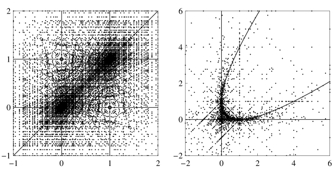
Figure 8.1. $U_{1^{5}}({\mathbb{Z}}^{\{2,3,5,7\}})\subset U_{1^{5}}({\mathbb{R}})$ and $U_{21^{3}}({\mathbb{Z}}^{\{2,3,5\}})\subset U_{21^{3}}({\mathbb{R}})$.

The sets $U_{\nu}({\mathbb{Z}}^{P})$ fit into standard geometrical considerations much better than the ${\mbox{\rm Polys}}_{\kappa}(P)$ do. For example, $U_{\nu}({\mathbb{Z}}^{P})$ lies in the $k$-dimensional real manifold $U_{\nu}({\mathbb{R}})$, while similar oversets are not as natural for ${\mbox{\rm Polys}}_{\kappa}(P)$. Figure 8.1 draws examples, directly related to Sections 3 and 4. In each case, $U_{\nu}({\mathbb{R}})$ is the complement in ${\mathbb{R}}^{2}$ of the drawn curves.

8.3. Covers

The fundamental groups of the complex manifolds $U_{\nu}({\mathbb{C}})$ are braid groups. Katz’s theory [9] of rigid local systems gives a whole hierarchy of covers of $U_{\nu}$ [12, 15]. The theory of Hurwitz varieties as presented in [1] likewise gives a another whole hierarchy of covers [16, 14]. In both cases, the covers have a topological description over ${\mathbb{C}}$, and this description forms the starting point of a more arithmetic description over ${\mathbb{Z}}$. In each case, the datum defining a cover determines a finite set $W$ of primes. The cover is then unramified except in characteristics $p\in W$. For these bad characteristics, the cover is typically wildly ramified.

Rather than enter theoretically into these two theories, we discuss next two representative examples, both with $\nu=21^{3}$ for uniformity. As coordinates, we work with $(u_{1,1},u_{1,2})=((1-v-u)/u,v/u)$ so that the right half of Figure 8.1 is the $u$-$v$ plane. Our current coordinates are related to the quantities of Section 4 by $u=u_{0}/u_{1}$ and $v=u_{\infty}/u_{1}$.

8.4. A Katz cover

The last half of [15] considers two Katz covers with bad reduction set $W=\{2,3\}$. The smaller of the two is captured by the explicit polynomial

$$f_{27}(u,v,x)=$$

$$\left(x^{3}-3dx+2ed\right)\left(x^{6}-15dx^{4}+40edx^{3}-45d^{2}x^{2}+24ed^{2}x-32e^{2}d^{2}+27d^{3}\right)^{4}$$

$$-432vd\left(x^{4}-6dx^{2}+8edx-3d^{2}\right)^{6},$$

with abbreviations $d=u^{2}+v^{2}-2uv-2u-2v+1$ and $e=u+v-1$. The polynomial discriminant factors,

$$D_{27}(u,v)=2^{840}3^{270}u^{102}v^{126}d^{234}.$$

The Galois group of $f_{27}(u,v,x)\in{\mathbb{Z}}[u,v][x]$ is the orthogonal group $O_{6}^{-}({\mathbb{F}}_{2})\subset S_{27}$ of order $51,840=2^{7}\,3^{4}\,5$. The specialization set $U_{21^{3}}({\mathbb{Z}}^{\{2,3\}})$ has order $60+169=229$ from Table 5.2. This specialization process produces 193 number fields with Galois group $O_{6}^{-}({\mathbb{F}}_{2})$, 15 with Galois group the index two simple group $O_{6}^{-}({\mathbb{F}}_{2})^{+}$, and other number fields with various smaller Galois groups [15].

Covers in the Katz hierarchy typically yield Lie-type Galois groups, like in this example, with bad reduction set $W$ containing at least two primes. By varying the Katz cover, a single fixed specialization point $u\in U_{\nu}({\mathbb{Z}}^{W})$ with $|W|\geq 2$ can be expected to yield infinitely many different fields ramified within $W$.

8.5. A Hurwitz cover

Many Hurwitz covers of $U_{21^{3}}$ with bad reduction set $W=\{2,3,5\}$ are studied in [14]. One such cover has degree $36$ and can be given via equations as follows. The cover $X$ can be given coordinates $x$ and $y$ so that the map to $U_{21^{3}}$ takes the form

$$u = -\frac{32\left(x^{2}-2y\right)^{5}}{27y(x-y)^{4}\left(8x^{3}-x^{2}-18xy+27y^{2}+2y\right)},$$

$$v = -\frac{\left(4x^{3}-x^{2}+18xy+27y^{2}-4y\right)^{2}\left(2x^{4}-5x^{2}y+6xy^{2}-y^{3}+2y^{2}\right)}{27y(x-y)^{4}\left(8x^{3}-x^{2}-18xy+27y^{2}+2y\right)}.$$

Eliminating $y$ gives $f_{36}(u,v,x)\in{\mathbb{Z}}[u,v][x]$ with $x$-degree $36$ and $1125$ terms. Its discriminant is

$$D_{36}(u,v)=-2^{337}3^{513}5^{750}u^{53}v^{13}d^{22}C(u,v)^{2},$$

with the complicated polynomial $C(u,v)\in{\mathbb{Z}}[u,v]$ not contributing to field discriminants of specializations. The specialization set $U_{21^{3}}({\mathbb{Z}}^{\{2,3,5\}})$, drawn as the right half of Figure 8.1, has order $1927+1020=2947$ from Table 4.1. The specialization process produces 2652 number fields with Galois group $S_{36}$, 42 number fields with Galois group $A_{36}$, and others with various smaller Galois groups, all with bad reduction set exactly $\{2,3,5\}$.

Covers in the Hurwitz hierarchy typically yield alternating or symmetric groups, like in this example, with bad reduction set $W$ containing all primes dividing the order of some nonabelian finite simple group, thus at least three primes. Here again, by varying the cover, a single fixed specialization point $u\in U_{\nu}({\mathbb{Z}}^{W})$ can give many different fields ramified within $W$.

8.6. Constraining wild ramification

Let $K_{u}$ be an algebra obtained by specializing a cover with bad reduction set $W$ at a point $u$ with bad reduction set $P$. Then the typical behavior of $p$-adic ramification in $K_{u}$ is as follows:

$$\begin{array}[]{l | ll}&p\in P&p\not\in P\\ \hline\cr p\in W&\mbox{very wild}&\mbox{slightly wild}\\ p\not\in W&\mbox{tame}&\mbox{none}\\ \end{array}$$

To illustrate the distinction between “very wild” and “slightly wild”, we specialize the Katz cover $f_{27}(u,v,x)$ and the Hurwitz cover $f_{36}(u,v,x)$ at the $15$-element set $U_{21^{3}}({\mathbb{Z}}^{\{2\}})$ appearing as black vertices in Figure 2.1:

$$\begin{array}[]{rrr|rrr|rrr}u_{0}&u_{1}&u_{\infty}&\lx@intercol\hfil d_{27}(u,v)\hfil\lx@intercol\vrule\lx@intercol&\lx@intercol\hfil d_{36}(u,v)\hfil\lx@intercol\\ \hline\cr 8&1&1&2^{88}3^{32}&2^{98}3^{36}&\bullet 2^{86}3^{34}&-2^{127}3^{39}5^{30}&-2^{127}3^{43}5^{30}&-2^{118}3^{39}5^{30}\\ -4&1&1&2^{80}3^{36}&2^{84}3^{36}&2^{80}3^{36}&2^{114}3^{39}5^{30}&2^{112}3^{39}5^{30}&\bullet{-2^{100}3^{25}5^{28}}\\ 2&1&1&2^{88}3^{36}&2^{88}3^{30}&2^{82}3^{30}&-2^{115}3^{39}5^{30}&-2^{121}3^{39}5^{30}&-2^{118}3^{39}5^{30}\\ -2&-1&1&2^{98}3^{36}&2^{102}3^{34}&2^{96}3^{32}&-2^{137}3^{27}5^{30}&2^{137}3^{39}5^{30}&2^{134}3^{39}5^{30}\\ 2&-1&1&2^{98}3^{36}&2^{102}3^{36}&2^{96}3^{36}&2^{137}3^{35}5^{30}&-2^{137}3^{27}5^{30}&2^{134}3^{39}5^{30}\end{array}$$

On a given row starting with $(u_{0},u_{1},u_{\infty})$, the $(u,v)$ in the second and third blocks are, in order, $(u_{0},u_{\infty})/u_{1}$, $(u_{1},u_{0})/u_{\infty}$, and $(u_{\infty},u_{1})/u_{0}$.

Field discriminants of the specializations are as indicated by the table. As $(u,v)$ runs over all of $U_{21^{3}}({\mathbb{Z}}^{\{2,3\}})$ one gets discriminants $d_{27}(u,v)=2^{a}3^{b}$ with $a\in[24,102]$ and $b\in[26,60]$. Restricting to $U_{21^{3}}({\mathbb{Z}}^{\{2\}})$, the maximum $a$ appearing is not reduced at all, while the maximum $b$ is reduced from $60$ to $36$. Similarly, as $(u,v)$ runs over all of $U_{21^{3}}({\mathbb{Z}}^{\{2,3,5\}})$, one gets discriminants $d_{36}(u,v)=\pm 2^{a}3^{b}5^{c}$ with $a\in[40,137]$, $b\in[7,72]$, and $c\in[18,61]$. Restricting to $U_{21^{3}}({\mathbb{Z}}^{\{2\}})$, $a_{\rm max}$ is not reduced at all, while $b_{\rm max}$ is reduced from $72$ to $39$ and $c_{\rm max}$ is reduced from $61$ to $30$. This distinction between “very wild” and “slightly wild” makes all the sets ${\mbox{\rm Polys}}_{\kappa}(P)$ of interest in the applications, not just the ones where $P$ is large enough to contain the bad reduction set $W$ of a cover.

8.7. Explicit examples

To give completely explicit examples of number fields constructed using the specialization points, we continue the previous subsection. The fifteen specializations of $f_{27}(u,v,x)$ in the table all have Galois group $O_{6}^{-}({\mathbb{F}}_{2})$ except the bulleted one, which has Galois group the simple index two subgroup. A presentation for this field $K_{27,1/8,1/8}$ is ${\mathbb{Q}}[x]/g_{27}(x)$ with

$$g_{27}(x) = x^{27}-9x^{26}+21x^{25}+53x^{24}-288x^{23}+1628x^{21}-1164x^{20}-5409x^{19}$$

$$+5681x^{18}+12159x^{17}-14793x^{16}-20548x^{15}+25764x^{14}+30324x^{13}$$

$$-36220x^{12}-42249x^{11}+48465x^{10}+50819x^{9}-61773x^{8}-44220x^{7}$$

$$+64172x^{6}+23712x^{5}-48024x^{4}-5725x^{3}+22509x^{2}+147x-5045.$$

Similarly, the fifteen specializations of $f_{36}(u,v,x)$ in the table all have Galois group $S_{36}$ except the bulleted one, for which the Galois group is intransitive. A presentation for this algebra $K_{36,-1/4,-1/4}$ is ${\mathbb{Q}}[x]/(g_{10}(x)g_{13}(x^{2}))$ with

$$g_{10}(x) = x^{10}-4x^{9}+2x^{8}+8x^{7}-8x^{6}+8x^{5}-20x^{4}-10x^{2}+80x-60,$$

$$g_{13}(x) = x^{13}-44x^{12}+728x^{11}-5256x^{10}+15240x^{9}-5320x^{8}-41620x^{7}$$

$$+72280x^{6}-33940x^{5}-4320x^{4}-8760x^{3}+20480x^{2}-6140x+480.$$

The field ${\mathbb{Q}}[x]/g_{10}(x)$ has Galois group $S_{10}$ and discriminant $2^{25}3^{6}5^{5}$ while for ${\mathbb{Q}}[x]/g_{13}(x)$ these invariants are $S_{13}$ and $2^{33}3^{9}5^{11}$. Despite the small exponents, these fields are wildly ramified not only at $2$, but also at $3$ and $5$.

8.8. Larger degrees

In larger degrees, the numerics of the sets $U_{\nu}({\mathbb{Z}}^{P})$ are reflected more clearly in the number fields constructed. For example, in a degree $202$ example of [14], the specializations at $u\in U_{21^{3}}({\mathbb{Z}}^{\{2,3,5\}})$ produce $2947$ distinct fields, all full in the sense of having Galois group all of $A_{202}$ or $S_{202}$, all wildly ramified at $2$, $3$, and $5$, and unramified elsewhere. We similarly expect $U_{21^{3}}({\mathbb{Z}}^{\{2,3,5\}})$ to be likewise responsible for exactly $2947$ distinct full fields in many degrees $m>202$. It seems possible that the Hurwitz construction accounts for all full fields in $NF_{m}(\{2,3,5\})$ for most of these degrees $m$.

As another example which gives a numerical sense of the asymptotics of this situation, consider the specialization set $U_{32768,1^{3}}({\mathbb{Z}}^{\{2,3,5\}})={\mbox{\rm Polys}}_{[32768]}(\{2,3,5\})$, chosen because it contains $s_{8,1}$ from Figure 7.1. From the generating function (7.1), this specialization set contains more than $7.46\times 10^{43}$ elements. One of the smallest degree covers of $U_{32678,1^{3}}$, in the language of [14, 16], comes from the Hurwitz parameter $(S_{5},(21^{3},32,221,5),(32768,1,1,1))$. This cover has degree exactly $(10^{32768}\cdot 20\cdot 15\cdot 24)/(60\cdot 120)=10^{32768}$. As $u$ ranges over the large set $U_{32768,1^{3}}({\mathbb{Z}}^{\{2,3,5\}})$ the specialized algebras $K_{u}$ are all ramified within $\{2,3,5\}$. Other Hurwitz parameters give this same degree and we expect that there are many full fields in $NF_{10^{32768}}(\{2,3,5\})$. The point for this paper is that polynomials with bad reduction within $\{2,3,5\}$ are an ingredient in the construction of these $K_{u}$. By way of contrast, it seems possible that $NF_{10^{32678}+1}(\{2,3,5\})$ is empty.

9. Future directions

9.1. Specialization sets $U_{\nu}[{\mathbb{Z}}^{P}]$ for general $\nu$

Let $\nu=(\nu_{1},\dots,\nu_{r})$ be a sequence of positive integers. For $F$ a field, let $\mbox{Conf}_{\nu}(F)$ be the set of tuples of disjoint divisors $(D_{1},\dots,D_{r})$ on the projective line over $F$, with $D_{i}$ consisting of $\nu_{i}$ distinct geometric points. The group $PGL_{2}(F)$ acts on $\mbox{Conf}_{\nu}(F)$ by fractional linear transformations. The object $\mbox{Conf}_{\nu}$ itself is a scheme which is smooth and of relative dimension $\sum\nu_{i}$ over $\mbox{Spec}({\mathbb{Z}})$.

There is a natural quotient scheme $U_{\nu}=\mbox{Conf}_{\nu}/PGL_{2}$. The map $\epsilon_{\nu}:\mbox{Conf}_{\nu}\rightarrow U_{\nu}$ induces a bijection $\mbox{Conf}_{\nu}(F)/PGL_{2}(F)\rightarrow U_{\nu}(F)$ whenever $F$ is an algebraically closed field. In the case that $\nu_{r-2}=\nu_{r-1}=\nu_{r}=1$, the action of $PGL_{2}(F)$ on $\mbox{Conf}_{\nu}(F)$ is free for all fields $F$, and the maps $\mbox{Conf}_{\nu}(F)/PGL_{2}(F)\rightarrow U_{\nu}(F)$ are always bijective. The general case is more complicated because there may be points in $\mbox{Conf}_{\nu}(F)$ for which the stablizer in $PGL_{2}(F)$ is nontrivial. The proofs of Theorems 4.1 and 5.1 involved the maps $\epsilon_{\nu}$ for $\nu=21^{2}$ and $\nu=31$ without using this notation. Via the coordinates $w$ and $j$ respectively, one has $U_{21^{2}}(F)=F^{\times}$ and $U_{31}(F)=F$ for $F$ of characteristic $>2$ and $>3$ respectively. The complications with fixed points are above $w=1$ and $j=0,1$.

For $P$ a finite set of primes, let $U_{\nu}[{\mathbb{Z}}^{P}]$ be the image of $\mbox{Conf}_{\nu}({\mathbb{Z}}^{P})$ in $U_{\nu}({\mathbb{Q}})$. The set $U_{\nu}[{\mathbb{Z}}^{P}]$ may be strictly smaller than the set $U_{\nu}({\mathbb{Z}}^{P})$ of scheme-theoretical $P$-integral points, as illustrated by the equalities $U_{21^{2}}[{\mathbb{Z}}^{P}]=T_{\infty,2,\infty}({\mathbb{Z}}^{P})\cup\{1\}$ and $U_{31}[{\mathbb{Z}}^{P}]=T_{3,2,\infty}({\mathbb{Z}}^{P})\cup\{0,1\}$, which hold respectively under the assumptions $\{2\}\subseteq P$ and $\{2,3\}\subseteq P$.

In this paper, we have focused on tabulating ${\mbox{\rm Polys}}_{\kappa}(P)$ to keep sets small and have a clear graph-theoretic interpretation. However from the point of view of Section 8, our actual problem has been the identification of $U_{\nu}({\mathbb{Z}}^{P})$ whenever $\nu_{r-2}=\nu_{r-1}=\nu_{r}=1$. The natural generalization is to identify $U_{\nu}[{\mathbb{Z}}^{P}]$ for general $(\nu,P)$. The Katz and Hurwitz theories of the previous section naturally give covers of general $U_{\nu}$ for general $\nu$.

The general problem of identifying $U_{\nu}[{\mathbb{Z}}^{P}]$ has the same character as the special case that we treat, but is technically more complicated because elements of $\mbox{Conf}_{\nu}({\mathbb{Z}}^{P})$ can no longer be canonically normalized by applying a fractional linear transformation. In the extreme case $\nu=(n)$ the complications become quite severe: describing the scheme $U_{n}$ is a goal of classical invariant theory, and explicit results become rapidly more complicated as $n$ increases.

The group $S_{n}$ acts naturally on the scheme $U_{1^{n}}$. Despite the normalization of three points to $0$, $1$, and $\infty$ in previous sections, the influence of this automorphism group has been visible. For example, the natural automorphism group of the left half of Figure 8.1 is $S_{5}$, and it acts transitively on the twelve components of $U_{1^{5}}({\mathbb{R}})$. An alternative viewpoint on $U_{\nu}$ for general $\nu=(\nu_{1},\dots,\nu_{r})$ is via the equation

(9.1) $$U_{\nu}=U_{1^{n}}/(S_{\nu_{1}}\times\cdots\times S_{\nu_{r}}).$$

For example, the left half of Figure 8.1 covers the right half via $U_{1^{5}}\rightarrow U_{21^{3}}$, $(s,t)\mapsto(u,v)=(s+t,(1-s)(1-t))$. The map is not surjective even on ${\mathbb{R}}$-points or ${\mathbb{Q}}_{p}$-points. The map is very far from far from surjective on the ${\mathbb{Z}}^{P}$-points of interest to us, and so the new $U_{\nu}$ present genuinely new arithmetic sets $U_{\nu}[{\mathbb{Z}}^{P}]$ to be identified, despite the tight relation (9.1). Birch and Merriman [2] proved, as part of a considerably larger theory, that the sets $U_{\nu}[{\mathbb{Z}}^{P}]$ are all finite. Their finiteness theorem was made effective by Evertse and Győry [8].

9.2. Descriptions of $U_{\nu}[{\mathbb{Z}}^{P}]$

The most straightforward continuation of this paper would be to completely identify more $U_{\nu}[{\mathbb{Z}}^{P}]$. Staying first in the context $\nu_{r-2}=\nu_{r-1}=\nu_{r}=1$, the direction needing most attention is general completeness results for the excellent $P$-units introduced in Section 6. Magma [3] already has the efficient command ExceptionalUnits giving complete lists of exceptional units. An extension of its functionality to $P$-units would immediately move many $U_{\nu}({\mathbb{Z}}^{P})$ currently in the second regime of expected completeness into the first regime of proved completeness. Leaving the context of $\nu_{r-2}=\nu_{r-1}=\nu_{r}=1$, there are many more $(\nu,P)$ for which complete identification of $U_{\nu}[{\mathbb{Z}}^{P}]$ is within reach, as it is only required that the normalization problem be resolved in some different way.

In the third regime of the introduction, where complete tabulation is impossible, there are still many questions to pursue. One would first like heuristic estimates on $|U_{\nu}[{\mathbb{Z}}^{P}]|$; the study of exceptional units in [11] looks to be a useful guide. The “vertical” direction of $P$ fixed and $\nu$ varying is interesting from the point of view of constructing number fields with larger degree and bounded ramification. In this direction it seems that close attention to constructional techniques like those of Section 7 may yield good lower bounds. In the “horizontal” direction of $\nu$ fixed and $P$ increasing, the Reduction Bound 2.1 becomes particularly important and upper bounds on $|U_{\nu}[{\mathbb{Z}}^{P}]|$ may be available. Finally, the $U_{\nu}[{\mathbb{Z}}^{P}]$ are not just bare sets to be tabulated or counted, one should also pay attention to their natural structures. Figure 8.1 suggests that in the horizontal direction the asymptotic distribution of $U_{\nu}[{\mathbb{Z}}^{P}]$ in $U_{\nu}({\mathbb{R}})$ may be governed by interesting densities. The asymptotic distribution of $U_{\nu}[{\mathbb{Z}}^{P}]$ in $U_{\nu}({\mathbb{Q}}_{p})$ is important for understanding the $p$-adic ramification of number fields constructed via covers, and may likewise be governed by densities.

References

- [1] José Bertin and Matthieu Romagny. Champs de Hurwitz. Mém. Soc. Math. Fr. (N.S.) No. 125-126 (2011), 219 pp.
- [2] B. J. Birch and J. R. Merriman. Finiteness theorems for binary forms with given discriminant. Proc. London Math. Soc. (3) 24 (1972), 385–394.
- [3] W. Bosma, J. J. Cannon, C. Fieker, A. Steel (eds.), Handbook of Magma Functions, Edition 2.19 (2012), 5478 pages.
- [4] F. B. Coghlan. Elliptic curves with condutor . Ph. D. Thesis, Manchester University (1967). Tables in: Modular Forms of One Variable IV. Springer Lecture Notes in Math. 476 (1975) pp. 123-134. Springer Verlag.
-
[5]
J. E. Cremona.
http://www.warwick.ac.uk/staff/J.E.Cremona/ftp/data/extra.html - [6] John W. Jones. Number fields unramified away from 2. J. Number Theory 130 (2010), no. 6, 1282–1291.
-
[7]
John W. Jones and David P. Roberts. A database of number fields. In preparation. Database at
http://hobbes.la.asu.edu/NFDB/ - [8] J.H. Evertse and K. Györy. Effective finiteness results for binary forms with given discriminant. Compositio Math. 79 (1991), no. 2, 169 204.
- [9] Nicolas Katz. Rigid Local Systems. Annals of Mathematics Studies, 139. Princeton University Press, Princeton, NJ, 1996. viii+223 pp.
- [10] Armin Leutbecher and Gerhard Niklash. On cliques of exceptional units and Lenstra’s construction of Euclidean fields. Number theory (Ulm, 1987), 150–178, Lecture Notes in Math., 1380, Springer, New York, 1989.
- [11] Gerhard Niklasch. Counting exceptional units. Journées Arithmétiques (Barcelona, 1995). Collect. Math. 48 (1997), no. 1-2, 195–207.
- [12] David P. Roberts. An construction of number fields. Number theory, 237–267, CRM Proc. Lecture Notes, 36, Amer. Math. Soc., Providence, RI, 2004.
- [13] by same authorFractalized cyclotomic polynomials. Proc. Amer. Math. Soc. 135 (2007), no. 7, 1959–1967.
- [14] by same authorHurwitz number fields. In preparation.
- [15] by same authorCovers of and number fields. In preparation.
- [16] David P. Roberts and Akshay Venkatesh. Hurwitz monodromy and full number fields. arXiv:1401.7379. Submitted.
- [17] B. M. M. de Weger. Solving exponential Diophantine equations using lattice basis reduction algorithms. J. Number Theory 26 (1987), no. 3, 325–367.