Visualization of atomic-scale phenomena in superconductors: application to FeSe

Abstract

We propose a simple method of calculating inhomogeneous, atomic-scale phenomena in superconductors which makes use of the wave function information traditionally discarded in the construction of tight-binding models used in the Bogoliubov-de Gennes equations. The method uses symmetry-based first principles Wannier functions to visualize the effects of superconducting pairing on the distribution of electronic states over atoms within a crystal unit cell. Local symmetries lower than the global lattice symmetry can thus be exhibited as well, rendering theoretical comparisons with scanning tunneling spectroscopy data much more useful. As a simple example, we discuss the geometric dimer states observed near defects in superconducting FeSe.

In the past two decades, two developments have spurred new interest in atomic-scale effects in superconductors. The first is the discovery of systems, like the high-$T_{c}$ cuprates, heavy fermion, and Fe-based superconductors, with very short coherence lengths $\xi$, which in the cuprates approach the unit cell size. The second is the ability to image atomic- and even sub-atomic scale features in scanning tunneling spectroscopy (STS). Comparison of such images with theory has sometimes been frustrating, since STS images often contain much more detail than that predicted by current calculations.

The success of the semiclassical theory of superconductivityEilenberger ; RainerSerene , which integrates out rapid oscillations of the pair wave function at the atomic-scale, has led to the widespread notion that atomic scale effects are irrelevant for superconductivity. However, observation of the electronic structure very near a defect or surface reflects directly the symmetry and structure of the superconducting order parameter, and can furthermore provide information on gap inhomogeneity, vortex structure, competing phases, and even the atomic-scale variation of the pairing interaction. Yet in the currently available method used to describe inhomogeneous phenomena, the Bogoliubov-de Gennes equations, atomic wave function information is typically integrated out by adopting a tight-binding model for the normal state electronic structure.

There is now a growing list of problems which seem to require atomic scale “details” beyond the BdG description usually employed. For example, STS images of underdoped cuprates show the existence of unusual incommensurate electronic modulations, proposed to represent real-space images of the pseudogap, which have alternating high and low intensity on O-centered bonds between neighboring Cu’sKapitulnik1 ; Davis_checkerboard1 ; Davis_checkerboard2 ; such effects cannot be captured by conventional models which include Cu states only. In general there has been a great recent effort to map out the intra-unit cell electronic structure of unconventional superconductors Lee ; Mesaros ; Hamidian ; Fujita ; Lawler . As a second example, there is still no consensus on the origin of the STS pattern around a Zn impurity in cuprates, which displays a central intensity maximum on the Zn site, unlike simple models of the response of a d-wave superconductor to a strong potentialZn . A popular explanation relies on “filter” effects which describe a nontrivial tunneling process from the surface to the CuO planeTing ; Martin , but while there is some support for these ideas from first principles calculations in the normal stateabinitioZn , there has been until now no way to include both superconductivity and the various atomic wave functions in the barrier layers responsible for the filterMarkiewicz . Finally, in Fe-based superconductors a variety of defect states observed by STS in FeSe, LiFeAs, NaFeAs and other materialssong11 ; grothe12 ; hanaguri12 ; zhou11 ; song12 ; pasupathy13 break the square lattice symmetry locally and therefore cannot be described by Fe-only lattice BdG calculations. These include so-called “geometrical dimer” structures aligned with the As or Se states at the surface. Note that in all of the above cases measurements sensitive to the LDOS at the surface are being used to analyze physics taking place several Å  beneath the surface, without a full understanding of the states involved in the tunneling process. Given that the STM tip almost always resides far away from the electronically active layers, these types of problems are to be expected for many superconducting materials.

In this work, we present a simple technique which restores the intra-unit cell information lost in the construction of the Bogoliubov-de Gennes Hamiltonian, including the degrees of freedom corresponding to other atoms in the unit cell, as well as neighboring cells. In weak-to-intermediate coupling systems, the method dramatically improves the ability of theory to quantitatively describe intra-unit cell problems, as we illustrate by presenting the solution to the FeSe problem described above. In strongly coupled systems like cuprates, it should still be valid for symmetry-related questions.

We first introduce the elementary expression for the local continuum Green’s function in terms of the BdG lattice Green’s function which is needed for the calculation of the local density of states (LDOS) relevant for the STS experiments. We then show that the nonlocal terms also contribute and can be important even for the local continuum LDOS. We present a tight-binding model for FeSe derived from Density Functional Theory (DFT) and corresponding Wannier basis. Within a 10-Fe-orbital BdG calculation, we calculate the response of the superconductor to a single pointlike impurity potential on an Fe site, and compare to the continuum LDOS calculated using the Wannier states. The geometric dimer states are shown to emerge naturally from this description. Finally, we discuss the approximations that we have made, as well as how the method can be improved and extended in the future.

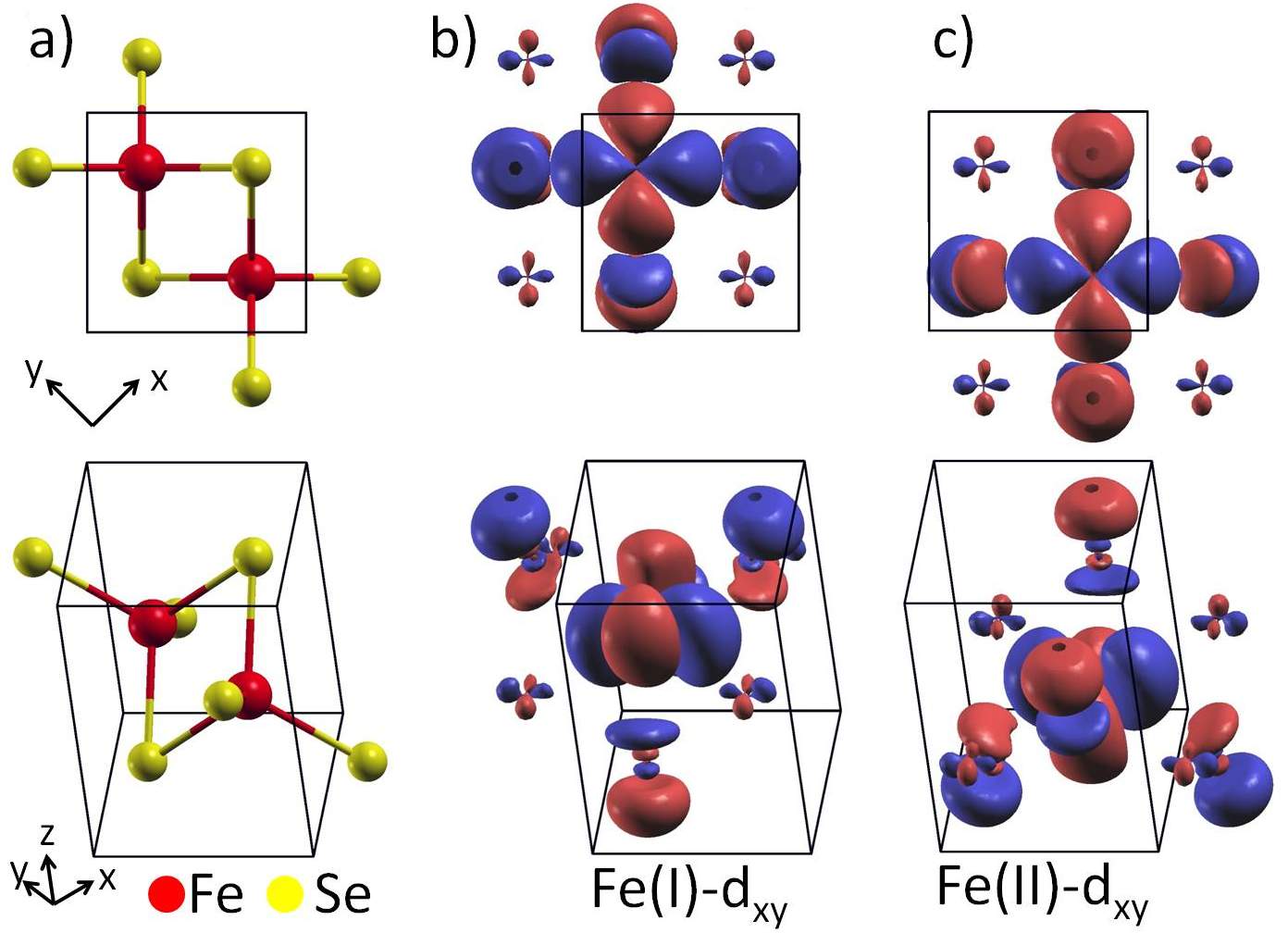
Figure 1: (color online) Isosurface plots of Fe-$d$ Wannier orbitals in FeSe at $0.03\,\text{bohr}^{-3/2}$; red and blue indicate phase of the wave function. a) (top) Top view of unit cell containing two Fe atoms (red) and two Se atoms (yellow), plus four Se exterior to unit cell; (bottom) side view of same cell. b) (top) Top view of $d_{xy}$ Wannier orbital on Fe(I) site; (bottom) side view of same orbital. c) Same as b) but on Fe(II) site. Images were produced with XCRYSDENKokalj .

Method. The tight binding model, while often treated as phenomenological, is in principle derived from Wannier orbitals based on first principles calculations. In order to preserve the desired mutual orthogonality of these orbitals, they are constructed from atomic wave functions on atoms in more than one unit cell, although they are exponentially localized. In a crystal with more than one type of atom per unit cell, Wannier orbitals may represent linear combinations of wave functions from more than one atomic species. Here we first construct from the DFT wave functions a basis $w_{{\mathbf{R}}\mu}({\mathbf{r}})$ using a projected Wannier method which preserves the local symmetry of the atomic statesKu_Wannier ; Anisimov . Here $\mu$ is an orbital index, ${\mathbf{R}}$ labels the unit cell, and ${\mathbf{r}}$ describes the continuum position. In Fig. 1, we show examples of the Wannier Fe-$d$ orbitals on the Fe(I) and Fe(II) sites derived for the homogeneous FeSe system, using the Fe-$d$ bands within the energy range $[-2.5,3]\,\text{eV}$ obtained from DFT using Wien2KBlaha . It is clear that, while these functions have features easily associated with the form of the corresponding atomic orbitals, they are considerably more complex, and involve significant contributions from the Se states integrated out in the downfolding, with clear differences between Fe(I) and Fe(II). These Wannier functions are used to derive the tight-binding model containing Fe site energies and hoppings in the usual way to yield the Hamiltonian $H_{0}=\sum_{\mathbf{RR^{\prime}},\mu\nu,\sigma}t_{\mathbf{{\mathbf{RR}^{\prime}}}}^{\mu\nu}c_{\mathbf{R}\mu\sigma}^{\dagger}c_{\mathbf{R^{\prime}}\nu\sigma}-\mu_{0}\sum_{\mathbf{R}\mu\sigma}n_{\mathbf{R}\mu\sigma}$, where $t_{\mathbf{RR^{\prime}}}^{\mu\nu}$ are hopping elements between orbitals $\mu$ and $\nu$ in unit cells $\mathbf{R}$ and $\mathbf{R}^{\prime}$. The full Hamiltonian for a superconductor in the presence of an impurity is therefore

$$H=H_{0}+H_{\text{BCS}}+H_{\text{imp}},$$ (1)

where

$$H_{\text{BCS}}=-\sum_{\mathbf{R},\mathbf{R^{\prime}},\mu\nu}\Delta_{\mathbf{RR^{\prime}}}^{\mu\nu}c_{\mathbf{R}\mu\uparrow}^{\dagger}c_{\mathbf{R^{\prime}}\nu\downarrow}^{\dagger}+H.c.,$$ (2)

with the superconducting order parameter $\Delta_{\mathbf{RR^{\prime}}}^{\mu\nu}=\Gamma^{\mu\nu}_{\mathbf{RR^{\prime}}}\langle c_{\mathbf{R^{\prime}}\nu\downarrow}c_{\mathbf{R}\mu\uparrow}\rangle$, and

$$H_{\text{imp}}=\sum_{\mu^{*}\sigma}V_{\text{imp}}c^{\dagger}_{\mathbf{R}^{*}\mu^{*}\sigma}c_{\mathbf{R^{*}}\mu^{*}\sigma},$$ (3)

where $\mathbf{R^{*}}$ is the impurity unit cell, $\mu^{*}$ in this term runs only over the 5$d$ orbitals associated with the impurity Fe site, and for simplicity we have taken the impurity potential $V_{\text{imp}}$ to be nonmagnetic and proportional to the identity in the orbital basis. Here $\Gamma_{\mathbf{RR^{\prime}}}^{\mu\nu}$ is the pairing interaction in orbital and real space. The inhomogeneous mean field BdG equations for this Hamiltonian may now be solved by diagonalization with the auxiliary self-consistency equation for the gap $\Delta_{{\mathbf{RR^{\prime}}}}^{\mu\nu}$ to obtain the BdG eigenvalues $E_{n\sigma}$ and eigenvectors $u_{n\sigma}$ and $v_{n\sigma}$. From these we can construct the usual retarded lattice Green’s function

$$G^{\mu\nu}_{\sigma}({\mathbf{R}},{\mathbf{R}}^{\prime};\omega)\!=\!\sum_{n}\!\left(\frac{u^{n\sigma}_{{\mathbf{R}}\mu}u^{n\sigma*}_{{\mathbf{R}}^{\prime}\nu}}{\omega-E_{n\sigma}+i0^{+}}+\frac{v^{n-\sigma}_{{\mathbf{R}}\mu}v^{n-\sigma*}_{{\mathbf{R}}^{\prime}\nu}}{\omega+E_{n-\sigma}+i0^{+}}\right).$$ (4)

Under a wide set of conditionsHamman , an STS experiment at bias $V=\omega/e$ measures the local density of states $\rho({\mathbf{r}},\omega)\equiv-\frac{1}{\pi}\mathop{\text{missing}}{Im}G({\mathbf{r}},{\mathbf{r}};\omega)$, related to the retarded continuum local Green’s function $G({\mathbf{r}},{\mathbf{r}}^{\prime};\omega)$.

To relate the lattice and continuum Green’s functions, one simply performs a basis transformation from the lattice operators $c_{{\mathbf{R}}\mu\sigma}$ to the continuum operators $\psi_{\sigma}({\mathbf{r}})=\sum_{{\mathbf{R}}\mu}c_{{\mathbf{R}}\mu\sigma}w_{{\mathbf{R}}\mu}({\mathbf{r}})$ where the Wannier functions $w_{{\mathbf{R}}\mu}({\mathbf{r}})$ are the matrix elements,

$$G({\mathbf{r}},{\mathbf{r}}^{\prime};\omega)=\sum_{{\mathbf{R}},{\mathbf{R}}^{\prime},\mu,\nu}\hskip-5.69046ptG^{\mu\nu}({\mathbf{R}},{\mathbf{R}}^{\prime};\omega)w_{{\mathbf{R}}\mu}({\mathbf{r}})w^{*}_{{\mathbf{R}}^{\prime}\nu}({\mathbf{r}}^{\prime}).$$ (5)

Note that even the local continuum Green’s function $G({\mathbf{r}},{\mathbf{r}};\omega)$ includes nonlocal and orbitally nondiagonal lattice Green’s function terms $G^{\mu\neq\nu}({\mathbf{R}}\neq{\mathbf{R}}^{\prime};\omega)$.

Application to FeSe. To illustrate the utility of this new method, we consider the general question of impurity states in Fe-based superconductors, which often exhibit unusual spatial forms. In particular, geometric dimers, high intensity conductance or topographic features localized on the sites of the two pnictide or chalcogenide atoms neighboring an Fe site, are ubiquitous in a number of Fe-based materials. It is not known whether these defects are Fe vacancies, adatoms or site switching, but they seem to be centered on a given Fe(I) or Fe(II) site, as imaged by STM topography, and it is natural to assume that the impurity state is coupled to the pnictide or chalcogenide atoms closest to the surface, i.e. the defects are oriented one way or another according to whether they are centered on Fe(I) or Fe(II). We consider here the effect of a repulsive potential on the Fe site, to crudely model a vacancy, site switching, or adatom, in the FeSe material ($T_{c}=8\,\text{K}$).

We now consider the form of the superconducting gap, which is not well-established for this system. The STS tunneling for thin films of FeSe on graphite is V-shaped at low energies, implying the presence of gap nodes or small minimum gap. We note, however, that Ref. DLFeng, has proposed that nodes may arise from a weak SDW state present in these films. This scenario is indeed consistent with the $\sim 16a_{0}$ long “electronic dimers”, high intensity spots observed with axes aligned at 45 degrees with respect to the geometrical dimers, which have been interpreted as emergent defect states in an ordered magnetic phaseNavarro_cigar . However since we are primarily interested in exhibiting the local $C_{4}$ symmetry breaking effects due to ligand atoms possible within our current method, we ignore the possible effects of magnetism in this work, and calculate the real space pair potentials $\Gamma_{\mathbf{RR}^{\prime}}^{\mu\nu}$ within the random phase approximation (RPA) using the 10-orbital tight-binding band structure with $U=0.90\,\text{eV}$ and $J=U/4$, footnote following the procedure described in Ref. Navarro_LiFeAs, . The 10-orbital BdG equations are then solved on $15\times 15$ unit cell lattices with stable solutions found through iterations of the self-consistency equation for the real space gaps $\Delta_{\mathbf{RR^{\prime}}}^{\mu\nu}=\Gamma_{\mathbf{RR}^{\prime}}^{\mu\nu}\sum_{n}u_{\mathbf{R}\mu}^{n}v_{\mathbf{R^{\prime}}\nu}^{n*}f(E_{n})$, where $\sum_{n}$ denotes summation over all eigenstates $n$. When calculating the Green’s function we use $20\times 20$ supercells to acquire spectral resolution of order $\sim 0.5\,\text{meV}$. The superconducting ground state is found to be of the usual multiband $s_{\pm}$ type. Its DOS, shown as the red curve in the inset of Fig. 2(a), reflects the several different orbital gaps in the problem, and bears a striking resemblance to the nearly V-shaped conductance observed in experimentsong11 . Note, however, that the overall gap magnitude is much larger than in experiment, since we have chosen artificially large interaction parameters to deliberately create a unrealistically large gap, so that impurity bound states may be more clearly visualized within our numerical resolution. Since the normal state density of states for this material is flat at low energies, we do not expect this to alter our results qualitatively, although the exact value of the impurity potential which creates a bound state for a realistic gap size will change. Finally, we observe that the choice of method used to calculate the gap does not influence our qualitative results, e.g. a single constant next-nearest neighbor pair potential that gives an $s_{\pm}$ state is sufficient (see Supplement Material).

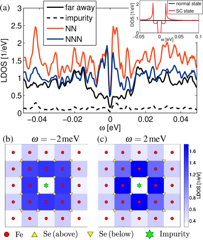
Figure 2: (color online) (a) density of states in SC state (inset: without impurity), far from impurity (black), at impurity site (black, dashed), on nearest neighbor site (orange [light gray]) and on next-nearest neighbor site (blue [dark gray]), calculated with a tetrahedron method using $40\times 40$ supercells. (b) resonant state real space BdG patterns at $\omega=-2\,\text{meV}$ and (c) $\omega=2\,\text{meV}$.

Single impurity in FeSe. We now add a single impurity to the system, of strength $V_{\text{imp}}=5\,\text{eV}$ in all orbital channels $\mu$, which creates an impurity bound state within the spectral gap at $\pm\Omega_{0}\simeq 2\,\text{meV}$ (Fig. 2(b)). The value chosen for this potential is not based on a microscopic description of a particular defect, but merely to create an in-gap bound state, to illustrate the method. Such bound states are not universal, but depend on the electronic structure of the host, impurity potential details, and gap functions, as has been emphasized in Refs. HKM_review, ; Vekhter1imp, . The structure of this complex bound state extends above and below the Fe plane, as can now be visualized by the current method.

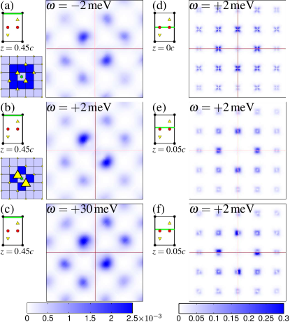
Figure 3: (color online) xy cuts through continuous 3D LDOS$(x,y,z;\omega)$ in $(\text{eV}\,\text{bohr}^{3})^{-1}$ at at the surface, $z=0.45c$ and different energies (a) $\omega=-2\,\text{meV}$, (b) $2\,\text{meV}$, (c) $30\,\text{meV}$, and heights at (close to) the Fe-plane $z=0c$ (d), $z=0.05c$ (e,f) and the same energy $2\,\text{meV}$, where the $c$-axis lattice constant is $c=10.44\,\text{bohr}$. All maps are calculated from Eq. (5) except for (e), which includes only the local (${\mathbf{R}}={\mathbf{R}}^{\prime}$, $\mu=\nu$) contributions. The schematic side views of the unit cell indicate the $z$-value of the cut (green line) relative to the Fe (red circles) and Se (yellow triangle) positions. The cartoon left of (a,b) explains the LDOS patterns in terms of the resonant nearest neighbor Fe Wannier orbitals (compare Fig. 2(b,c)) and their upper Se tails. Thin red lines are directed along Fe-Fe bonds through the central impurity site, and the black border indicates the extent of the 5$\times$5 Fe region.

In Fig. 2 (b), (c), we show first the local lattice density of states $\rho_{\text{BdG}}({\mathbf{R}},\omega)\equiv-\frac{1}{\pi}\mathop{\text{missing}}{Im}\,G({\mathbf{R}},{\mathbf{R}};\omega)$ obtained at the positive and negative resonance energies within a conventional 10-Fe orbital BdG calculation. As is clear, both resonance patterns are $C_{4}$ symmetric as they must be for the tetragonal FeSe system, and do not resemble any defect states imaged in STS experiments on this system. The orthorhombic distortion of FeSe at low temperatures has been disregarded in our work, as it cannot account for the $C_{4}$ to $C_{2}$ symmetry breaking close to the impurity with axis 45 degrees away from the Fe-Fe bond. In Fig. 3, we finally plot the analogous continuum LDOS $\rho({\mathbf{r}},\omega)\equiv-\frac{1}{\pi}\mathop{\text{missing}}{Im}\,G({\mathbf{r}},{\mathbf{r}};\omega)$, which extends in three dimensions, although the set of ${\mathbf{R}}$ considered in Eq. (5) lies in a 2D plane, due to the 3D spatial extent of the Wannier functions. Cuts at various heights $z$ from $z=0$ in the Fe-Fe plane to a point very close to the Se plane are shown. As expected from Fig. 2 (b), (c), in the Fe plane $\rho({\mathbf{r}},\omega)$ is still $C_{4}$ symmetric (Fig. 3 (d)), but when one increases $z$ the local placement of the Se atoms breaks this symmetry to $C_{2}$, as clearly seen in Fig. 3 (a-c) for $z$ close to the surface where the STM tip is roughly located. In our result, the dimer from the large LDOS close to the NN (up) Se atoms is visible at all energies, but there is some signicant variation with energy in the intensity on the NNN (up) Se, yet this may change according to the details of the actual defect potential. Looking at the corresponding Fe-only BdG LDOS patterns in Fig. 2 (b-c), also shown as cartoon in Fig. 3 (a-b), suggests a simple explanation of the patterns, namely that intensity maxima occur on those Se sites associated with the resonant Fe Wannier orbitals, with intensities on these Se sites adding constructively. Of course, deviations are in general to be expected, since simply adding intensities from resonant sites neglects contributions from nonresonant ones, as well as from nonlocal terms $\mathbf{R}\neq\mathbf{R^{\prime}},\nu\neq\mu$ in the continuum Green’s function arising in Eq. (5). The importance of these latter terms is illustrated in Fig. 3(e), where the local, orbitally diagonal contributions are plotted alone for a cut just above the Fe plane. The true, significant symmetry breaking is only recovered in the full result Fig. 3(f).

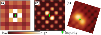
Figure 4: (color online) Topography of impurity state: comparison of topograph with setpoint bias $+6\,\text{mV}$ for (a) BdG calculation of impurity state as in Fig. 2(b); and (b) BdG-Wannier calculation of same impurity state. In (c) we reproduce the experimental topograph from Ref. song12, , rotated such that the directions of the lattice vectors match in all images.

Discussion. To illustrate the dramatic improvements provided by our proposed approach we compare in Fig. 4 the topographs of the impurity state calculated within the BdG and BdG-Wannier approaches with the experimentally observed song12 geometrical dimer footnote2 . The BdG-Wannier approach of course will also reproduce the experimentally observed song12 90 degree rotation of the dimer when the impurity potential is moved from the Fe(I) sublattice to the Fe(II) sublattice. Other comparisons with experiment are difficult, as detailed spectral features of these states are not yet published. The low-energy resonant state created by the opening of the superconducting gap (Fig. 3(a,b,d,f)), and a nonresonant impurity state with similar patterns visible at higher energy (Fig. 3(c)), broader in energy due to its coupling to the metallic continuum, represent predictions which can be tested by experiment when spectral data are available.

Conclusions. We have introduced a method to enable theoretical visualization of inhomogeneous states in superconductors, combining traditional solutions of the Bogoliubov-de Gennes equations with a first principles Wannier analysis. The method not only enables a much higher spatial resolution, but also captures the local symmetry internal to the unit cell of the crystal. Furthermore the method incorporates the nonlocal lattice Green’s function contributions, which we have demonstrated to be of qualitative importance. As an example, we showed how “geometric dimer” impurity states seen in Fe-based superconductors can be understood as consequence of simple defects located on the Fe site due to the hybridization with the pnictogen/chalcogen states. In terms of both symmetry and higher spatial resolution, the result obtained with the method introduced here represents a qualitative improvement over conventional BdG investigations (Fig. 4), and opens a new window on the theoretical analysis of atomic scale phenomena in superconductors.

Acknowledgements. The authors are grateful to B.M. Andersen, H.P.-Cheng, M.N. Gastiasoro, J. Hoffman, W. Ku, C.-L. Song, and Y. Wang for useful discussions. PC, AK, and PJH were supported by DOE DE-FG02-05ER46236, CC by NSFC 11274006, and TB by DOE CMCSN DE-AC02-98CH10886 and as a Wigner Fellow at the Oak Ridge National Laboratory. The authors are grateful to W. Ku for use of his Wannier function code.

References

- (1) G. Eilenberger, Z. Phys. 214, 195 (1968).
- (2) J. Serene and D. Rainer, Phys. Rep. 104, 221 (1983).
- (3) C. Howald, H. Eisaki, N. Kaneko, M. Greven, and A. Kapitulnik, Phys. Rev B 67, 014533 (2003).
- (4) T. Hanaguri, C. Lupien, Y. Kohsaka, D. -H. Lee, M. Azuma, M. Takano, H. Takagi and J. C. Davis, Nature 430 (2004).
- (5) Y. Kohsaka, C. Taylor, K. Fujita, A. Schmidt, C. Lupien, T. Hanaguri, M. Azuma, M. Takano, H. Eisaki, H. Takagi, S. Uchida, and J. C. Davis, Science 315, 1380 (2007).
- (6) J. Lee, M. P. Allan, M. A.Wang, J. Farrell, S. A. Grigera, F. Baumberger, J. C. Davis, A. P. Mackenzie, Nat. Phys. 5, 800 (2009).
- (7) A. Mesaros, K. Fujita, H. Eisaki, S. Uchida, J. C. Davis, S. Sachdev, J. Zaanen, M. J. Lawler, Eun-Ah Kim, Science 333, 426 (2011).
- (8) M. H. Hamidian, I. A. Firmo, K. Fujita, S. Mukhopadhyay, J. W. Orenstein, H. Eisaki, S. Uchida,M. J. Lawler, E.-A. Kim, J. C. Davis, New J. Phys. 14 053017 (2012).
- (9) K. Fujita et al., arXiv:1404.0362.
- (10) M. J. Lawler, K. Fujita, Jhinhwan Lee, A. R. Schmidt, Y. Kohsaka, Chung Koo Kim, H. Eisaki, S. Uchida, J. C. Davis, J. P. Sethna and E.-A. Kim, Nature 466, 347 (2010).
- (11) For reviews see A. V. Balatsky, I. Vekhter, and J.-X. Zhu, Rev. Mod. Phys. 78, 373 (2006); H. Alloul, J. Bobroff, M. Gabay and P.J. Hirschfeld, Rev. Mod. Phys. 81, 45 (2009).
- (12) J.-X. Zhu, C. S. Ting, and C. R. Hu, Phys. Rev. B 62, 6027 (2000).
- (13) I. Martin, A. V. Balatsky, and J. Zaanen, Phys. Rev. Lett. 88, 097003 (2002).
- (14) L.-L. Wang, P. J. Hirschfeld, and H.-P. Cheng, Phys. Rev. B 72, 224516 (2005).
- (15) Note J. Nieminen et al., Phys. Rev. B 80, 134509 (2009) discussed the tunneling in cuprates with a formalism similar in spirit to the one used here, but did not apply it to inhomogeneous problems, while Dell’Anna et al., Phys. Rev. B 71, 064518 (2005) used Gaussian wave functions to suppress large momentum contributions in the quasiparticle interference pattern.
- (16) C.-L. Song, Y.-L. Wang, P. Cheng, Y.-P. Jiang, W. Li, T. Zhang, Z. Li, K. He, L. Wang, J.-F. Jia, H.-H. Hung, C. Wu, X. Ma, X. Chen, and Q.-K. Xue, Science 332, 1410 (2011).
- (17) S. Grothe, S. Chi, P. Dosanjh, R. Liang, W. N. Hardy, S. A. Burke, D. A. Bonn, and Y. Pennec, Phys. Rev. B 86, 174503 (2012).
- (18) T. Hanaguri, private communication.
- (19) X. Zhou, C. Ye, P. Cai, X. Wang, X. Chen, and Y. Wang, Phys. Rev. Lett. 106, 087001 (2011).
- (20) C.-L. Song, Y.-L. Wang, Y.-P. Jiang, L. Wang, K. He, X. Chen, J. E. Hoffman, X.-C. Ma, and Q.-K. Xue, Phys. Rev. Lett. 109, 137004 (2012).
- (21) E.P. Rosenthal, E.F. Andrade, C.J. Arguello, R.M. Fernandes, L.Y. Xing, X.C. Wang, C.Q. Jin, A.J. Millis, and A.N. Pasupathy, Nat. Phys. 10, 225 (2014).
- (22) A. Kokalj, Comp. Mater. Sci. 28 155 (2003).
- (23) W. Ku et al., Phys. Rev. Lett. 89, 167204 (2002).
- (24) V. I. Anisimov et al., Phys. Rev. B 71, 125119 (2005).
- (25) P. Blaha et al., Comput. Phys. Commun. 147, 71 (2002).
- (26) J. Tersoff and D.H. Hamman, Phys. Rev. B 31, 805(1985).
- (27) S.Y.Tan, M.Xia, Y.Zhang, Z.R.Ye, F.Chen, X.Xie, R.Peng, D.F.Xu, Q.Fan, H.C.Xu, J.Juan, T.Zhang, X.C.Lai, T.Xiang, J.P.Hu, B.P.Xie, D.L.Feng, Nat. Mat. 12, 634 (2013).
- (28) M. N. Gastiasoro, P. J. Hirschfeld, and B. M. Andersen, Phys. Rev. B, 89, 100502(R) (2014).
- (29) M.N. Gastiasoro, P.J. Hirschfeld, and B.M. Andersen, Phys. Rev. B 88, 220509 (2013).
- (30) Note that the is defined here to include screening processes not included in the RPA (N. Bulut and D.J. Scalapino, Phys. Rev. B47, 2742 (1993)), and is consequently lower than values calculated from first principles.
- (31) P.J. Hirschfeld, M.M. Korshunov, and I.I. Mazin, Rep. Prog. Phys. 74, 124508 (2011).
- (32) R. Beaird, I. Vekhter, J.-X. Zhu, Phys. Rev. B 86, 140507 (2012).
- (33) Simulating the STM topograph requires an integration over a setpoint energy bias range, as described in the Supplement Material.