Elastic properties of eta carbide ($\eta$-Fe₂C) from ab initio calculations. Application to cryogenically treated gear steel.

Abstract

The elastic properties of $\eta$-Fe₂C (eta carbide) have been determined from ab initio density functional theory (DFT) calculations using the generalized gradient approximation (GGA). The isotropic polycrystalline elastic modulus of $\eta$-Fe₂C has been calculated as the average of anisotropic single-crystal elastic constants determined from the ab initio simulations. The calculated polycrystalline elastic modulus was used to compute the elastic modulus of a case carburised gear steel subjected to shallow cryogenic treatment (SCT) and deep cryogenic treatment (DCT). This value was then compared with experimental values obtained from nanoindentation. The results confirmed that the changes in elastic modulus observed in the DCT steel can be attributed to the precipitation of $\eta$-Fe₂C. No changes in hardness have been observed between the SCT steel and the DCT steel. These data were then used to assess the surface contact fatigue behaviour of the SCT and DCT steels tested under elastohydrodynamic lubrication (EHL) conditions.

Introduction

$\eta$-Fe₂C (eta carbide) and $\varepsilon$-Fe_2.4C (epsilon carbide) are two transition compounds which occur in the microstructure of quenched steels during the initial stages of tempering Nakamura1986 . The precipitation of $\varepsilon$-Fe_2.4C is predominant in conventional heat treatments (quenching in oil at temperatures above $273\,\text{K}$) while $\eta$-Fe₂C precipitates during cryogenic (sub-zero) treatments, known as shallow when the quenching temperature is near $193\,\text{K}$ and deep when the quenching is performed at or near $77\,\text{K}$ Baldissera2008 ; Bensely2006 .

The application of cryogenic treatments to steel components such as tools Das2009 ; Das2010a ; Das2010 ; Firouzdor2008 ; Molinari2001 and gears Baldissera2008 ; Bensely2006 ; Baldissera2009 ; Baldissera2009a ; Bensely2007 ; Bensely2008 ; Bensely2009 ; Bensely2011 ; Manoj2004 ; Paulin1993 ; Preciado2006 ; Stratton2009 is justified by numerous claims that the wear and fatigue behaviour is significantly improved mainly due to three phenomena which occur at low temperatures Baldissera2009a : complete martensitic transformation, changes in the residual stresses and precipitation of nanometric carbides.

The microstructure of surface hardened steels commonly used to manufacture heavy-duty gears typically consists of tempered martensite, retained austenite and iron carbides. The complexity of this microstructure has lead to somewhat contradictory opinions regarding the role played by individual phases in wear and contact fatigue. An example for this is the influence of retained austenite and its optimum amount (a brief review can be found in PhD-Oila2003 ).

A better understanding of the role played by individual phases is necessary for reliable failure predictions and this requires that the mechanical properties of the phases involved are known. Experimental determination of these properties (i.e. elastic modulus, hardness, yield strength, etc.) can be difficult, on one hand because of the small size of the grains (the $\eta$-Fe₂C observed Meng1994 varies from 5 to 10 nm in cross-section and from 20 to 40 nm in length) and, on the other hand because some phases are not stable at room temperature (i.e., unalloyed Fe-C austenite). The structure of Fe-C austenite as well as a number of relevant properties have been computed by molecular dynamics Oila2009 but, to date no experimental or theoretical data exists for the elastic modulus of $\eta$-Fe₂C.

The lattice parameter of $\eta$-Fe₂C has been determined from ab initio calculations by various authors Ande2012 ; Bao2009 ; Faraoun2006 ; Lv2008 , its bulk modulus has also been calculated Faraoun2006 ; Lv2008 but the anisotropic single-crystal elastic constants have been computed only by Lv et al. Lv2008 .

Although, the mechanisms by which cryogenic treatments improve the wear resistance of steels are not completely understood it is believed Meng1994 that the precipitation of nanometric $\eta$-Fe₂C enhances the strength and toughness of the martensite matrix, similar to the reinforcement of composites with nanoparticles. Also, the precipitation of the nanometric carbides is accompanied by a reduction in residual stresses in martensite Preciado2006 . The proposed mechanism Meng1994 of $\eta$-Fe₂C formation at low temperatures involves a slight shift of carbon atoms from the equlibrium position due to lattice deformation.

In this work, we determined the structural and elastic properties of $\eta$-Fe₂C from first principles. These include the lattice parameters and the single-crystal elastic constants. The isotropic polycrystalline elastic moduli have been calculated as averages of single-crystal elastic constants using the Hill’s average Hill1952 .

The calculated elastic modulus for $\eta$-Fe₂C and the experimentally determined elastic modulus of martensite were used to estimate the elastic modulus of a gear steel subjected to two different cryogenic treatments: shallow (SCT) and deep (DCT), respectively by applying the rule of mixtures (Eq. 13). These data were then used to assess the contact fatigue behaviour of the steel tested under rolling/sliding elastohydrodynamic lubrication (EHL) conditions.

At the time of writing there is no published work on the wear behaviour of cryogenically treated gear steels under EHL conditions (in which most case carburised gears operate).

Ab initio calculations

The crystal structure of $\eta$-Fe₂C (Fig. 1) is orthorhombic Dirand1983 ; Hirotsu1972 ; Nagakura1981 ; Nakamura1986 , space group $Pnnm$ (58), with 6 atoms in the conventional unit cell: 4 Fe atoms and 2 C atoms. The Wyckoff positions of the atoms are Fe $4g$ $(x,0.25,0)$ and C $2a$ $(0,0,0)$. The experimentally measured lattice parameters Dirand1983 $a=4.704$ Å, $b=4.318$ Å and $c=2.830$ Å were used as initial values in the simulations. The ab initio spin-polarized calculations were performed employing the generalized gradient approximation (GGA) Perdew1996 as implemented in the Quantum-ESPRESSO package Giannozzi2009 , using atomic ultrasoft pseudopotentials Laasonen1993 within the density functional theory (DFT) Hohenberg1964 ; Kohn1965 . The use of generalized gradient approximation (GGA) is preferred because it correctly predicts the ferromagnetic body centred cubic (BCC) structure of Fe, while the local density approximation (LDA) incorrectly predicts its ground state to be nonmagnetic Jiang2008 .

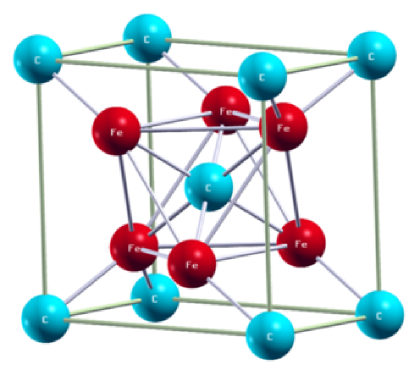
Figure 1: The orthorhombic unit cell of $\eta$-Fe₂C.

The Brillouin zone was sampled by constructing a $k$-points mesh following the Monkhorst-Pack scheme Monkhorst1976 in which the $k$-points are homogeneously distributed in rows and columns running parallel to the reciprocal vectors. The Brillouin zone integrations were performed using a Marzari-Vanderbilt method Marzari1999 with a Gaussian spreading of 0.005 Ry ($\sim 0.068$ eV). A mesh $6\times 7\times 10$ which gives 264 $k$-points in the Brillouin zone was selected for consequent calculations. Fig. 2 shows the energy values computed for different $k$-points meshes. For meshes containing 264 or more $k$-points all energy values lie within a window of $1\,\text{meV}$.

After the convergence tests, a plane wave kinetic-energy cutoff of 65 Ry ($\sim 884$ eV) and a charge density cutoff of 390 Ry ($\sim 5306$ eV) were found to be sufficient to converge the total energy to less than 5 meV/atom (Fig. 3).

Structural optimisation was performed by computing the total energy as a function of the unit cell volume by varying the $b/a$ and $c/a$ ratios while allowing the atomic coordinates to relax according to a conjugate-gradient scheme. The calculated energy was plotted versus the unit cell volume (Fig. 4) and fitted to the Murnaghan equation of state Murnaghan1944 .

The elastic constants, $c_{ij}$, of the orthorhombic unit cell were calculated by applying a small strain to the equilibrium lattice parameter and computing the total energy. The symmetric distortion matrix for an orthorhombic unit cell, $\vec{D}$, is given by Jiang2008 :

$$\vec{D}=\left(\begin{array}[]{ccc}1+\varepsilon_{1}&\varepsilon_{6}/2&\varepsilon_{5}/2\\ \varepsilon_{6}/2&1+\varepsilon_{2}&\varepsilon_{4}/2\\ \varepsilon_{5}/2&\varepsilon_{4}/2&1+\varepsilon_{3}\end{array}\right)$$ (1)

where $\varepsilon_{i}$ are the strain tensor components in Voigt notation. The elastic constants, $c_{ij}$, can be calculated from the Hook’s law. Fig. 5 shows an example of linear fitting of the calculated stress versus the applied strain. The corresponding elastic constant represents the slope of the fitted curve.

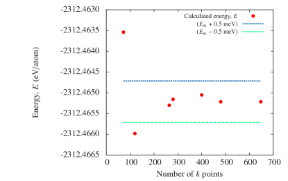
Figure 2: Energy function of the number of $k$-points in the Brillouin zone. $E_{m}=\text{the energy computed using the most dense mesh.}$

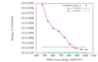
Figure 3: Energy convergence test for $\eta$-Fe₂C. $E_{m}=\text{the energy computed using the highest energy cutoff.}$

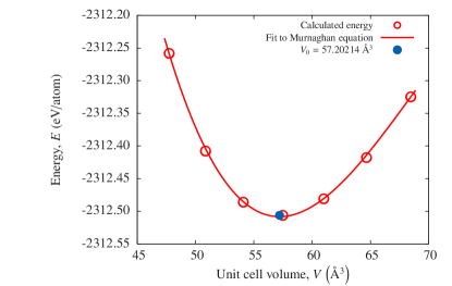
Figure 4: Calculated energy as a function of the $\eta$-Fe₂C unit cell volume.

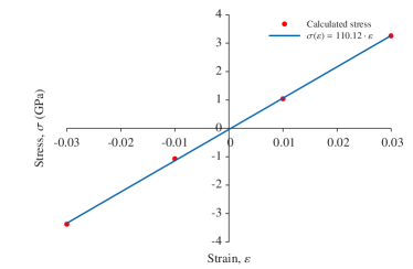
Figure 5: Calculation of elastic constant $c_{44}=110.12\,\text{GPa}$.

The polycrystalline bulk modulus $B$ (Eq. 2) and shear modulus $G$ (Eq. 3) can be calculated using the Hill’s average Hill1952 :

$$B=\dfrac{B_{Reuss}+B_{Voigt}}{2}$$ (2)

$$G=\dfrac{G_{Reuss}+G_{Voigt}}{2}$$ (3)

where $B_{Reuss}$ and $G_{Reuss}$ are given by Eq. 4 and 5 assuming uniform stress Reuss1929 and $B_{Voigt}$ and $G_{Voigt}$ are given by Eq. 6 and 7 assuming uniform strain Voigt1887 .

$$B_{Reuss}=\dfrac{1}{s_{11}+s_{22}+s_{33}+2\left(s_{12}+s_{23}+s_{13}\right)}$$ (4)

$$G_{Reuss}=\dfrac{15}{4\left(s_{11}+s_{22}+s_{33}-s_{12}-s_{23}-s_{13}\right)+3\left(s_{44}+s_{55}+s_{66}\right)}$$

(5)

$$B_{Voigt}=\dfrac{c_{11}+c_{22}+c_{33}+2\left(c_{12}+c_{23}+c_{13}\right)}{9}$$ (6)

$$G_{Voigt}=\dfrac{c_{11}+c_{22}+c_{33}-c_{12}-c_{23}-c_{13}}{15}+\dfrac{c_{44}+c_{55}+c_{66}}{5}$$

(7)

Table 1: Chemical composition of S156 steel, wt %.

C	Si	Mn	P	S	Cr	Mo	Ni
0.14-0.18	0.10-0.35	0.25-0.55	max. 0.015	max. 0.012	1.00-1.40	0.20-0.30	3.80-4.30

The elastic modulus, $E$, and the Poisson’s ratio, $\nu$, can be calculated using Eq. 8 and 9, respectively.

$$E=\dfrac{9BG}{3B+G}$$ (8)

$$\nu=\dfrac{3B/2-G}{3B+G}$$ (9)

Experimental

Tests were carried out on samples of S156 steel which had been carburised, quenched and surface ground. The chemical composition of the S156 steel is given in Table 1. The cryogenic treatments (SCT and DCT) were carried out at Frozen Solid UK after tempering at $190\,^{\circ}$C. The depth of the hardened case after grinding was approximately 1 mm. The surface finish measured by optical profilometry was $R_{a}=0.2-0.4$ $\mu$m, a value similar to that commonly obtained in gears. The retained austenite content has been measured by X-Ray diffraction using a XSTRESS 3000 (Stresstech Group) stress analyser. The values corresponding to the depth below surface at which the nanoindentation tests were carried out ($500$ $\mu$m) are given in Table 5.

Nanoindentation

The nanoindentation tests were carried out using a Hysitron Triboindenter with a Berkovich tip using a maximum applied load of $10\,\text{mN}$. After each indentation an area $5\times 5\,\mu\text{m}$ was scanned using the AFM (Atomic Force Microscope) of the triboindenter. Hardness, $H$ (Eq. 10) and elastic modulus, $E$ (Eq. 11 and 12) have been calculated using the Oliver-Pharr method Oliver1992 .

$$H=\dfrac{P_{max}}{A_{c}}$$ (10)

where:
	$P_{max}$ is the maximum indentation load
	$A_{c}$ is the projected area of tip-sample contact

$$E^{*}=\dfrac{1}{2}\sqrt{\dfrac{\pi}{A_{c}}}S$$ (11)

where:
	$E^{*}$ is the reduced contact modulus
	$S$ is the stiffness

$$\dfrac{1}{E^{*}}=\dfrac{1-\nu^{2}}{E}+\dfrac{1-\nu_{i}^{2}}{E_{i}}$$ (12)

where:
	$\nu$ and $\nu_{i}$ are the Poisson’s ratios of sample
	and indenter, respectively
	$E$ and $E_{i}$ are the Young’s moduli of sample
	and indenter, respectively

A total of 50 indentations have been performed on a polished cross section of each sample at a depth of approximately $500$ $\mu$m.

Surface contact fatigue

The surface contact fatigue tests have been carried out using a rig described in a previous publication Oila2005b . A number of six pairs of discs have been tested: two oil quenched, two shallow cryogenic treated and two deep cryogenic treated. In the conventional treatment the samples were oil quenched from $825\,^{\circ}$C, and tempered at $190\,^{\circ}$C.

In order to achieve an elliptical contact, one of the discs was crowned with a crown height of $5\,\text{mm}$, giving a crown radius of $250\,\text{mm}$. All contact fatigue tests have been carried out for $5\times 10^{5}\,\text{cycles}$ under a contact pressure $1.5\,\text{GPa}$, at a temperature of $60\,^{\circ}\text{C}$ and a speed of $1200\,\text{rev/min}$ with a slide-to-roll ratio of 0.33. The lubricant used was Valvoline HP Gear Oil 85W-140 1/5 GA and the calculated $\lambda$ ratio varied between 0.2 and 0.5.

The type of failure on all specimens, as observed by reflected light microscopy (RLM) and scanning electron microscopy (SEM) was predominantly micropitting (see Fig. 9). The distribution of the micropits inside the contact area, around the circumference of the disc, follows a uniform pattern which allows for the computation of the average percentage area of damage. The percentage damage has been measured by processing the images captured with a reflected light microscope, and it was determined as the average of 10 measurements taken in different locations chosen at random on the disc surface.

Results and discussion

Calculated properties of $\eta$-Fe₂C

The results calculated in this work have been compared with those obtained by others (where available). The calculated lattice parameters are generally in good agreement with values reported by other authors (Table 2).

Table 2: Lattice parameters (Å) of $\eta$-Fe₂C.

Source	$a$	$b$	$c$
This study	4.722	4.271	2.835
Hirotsu1972	4.704	4.318	2.830
Faraoun2006	4.687	4.261	2.830
Lv2008	4.677	4.293	2.814
Bao2009	4.651	4.258	2.805
Ande2012	4.708	4.281	2.824

Table 3: Elastic constants of $\eta$-Fe₂C (GPa).

Source	$c_{11}$	$c_{22}$	$c_{33}$	$c_{12}$	$c_{23}$	$c_{13}$	$c_{44}$	$c_{55}$	$c_{66}$
This study	323	340	378	189	158	136	110	97	136
Lv2008	310	346	296	170	216	170	64	148	157

The single-crystal elastic constants of $\eta$-Fe₂C are presented in Tabel 3. There are significant differences between the values calculated in the present study and those obtained by Lv et al. Lv2008 . The accuracy of the calculated elastic constants is strongly dependant on the accuracy of the self consistency runs and also on the convergence criteria of geometry optimizations for each distorted structure. In our calculations we have used a denser $k$-points mesh ($6\times 7\times 10$ compared to $6\times 6\times 9$ in Lv2008 ) and we imposed a convergence threshold of $10^{-8}$ Ry ($\sim 1.36\times 10^{-7}$ eV) while the convergence threshold used in Lv2008 was $10^{-5}$ eV.

The bulk modulus, $B$, (Tabel 4) calculated in this work agrees well with the values reported by Lv et al. Lv2008 and is about $8\%$ different than that reported by Faraoun et al. Faraoun2006 . For shear modulus, $G$, Poisson’s ratio, $\nu$, and elastic modulus, $E$, (Tabel 4) no data is available for comparison.

Table 4: Polycrystalline elastic moduli of $\eta$-Fe₂C (GPa).

Source	$B\,(\text{GPa})$	$G\,(\text{GPa})$	$E\,(\text{GPa})$	$\nu$
This study	223	147	362	0.23
Faraoun2006	243	-	-	-
Lv2008	226	-	-	-

Nanoindentation

The average elastic modulus of martensite, determined from nanoindentation tests carried out on the oil quenched samples was $E=203\,\text{GPa}$ and it was used as the reference value in the subsequent calculations of the volume fraction of carbides. The average elastic modulus of retained austenite was $E=175\,\text{GPa}$. Similar values were reported for the elastic modulus of Fe-C austenite from molecular dynamics calculations Oila2009 .

Table 5: Retained austenite measurements (%).

Sample	DCT	SCT	Oil quenched
Retained austenite (%)	$7.7\pm 0.6$	$9.3\pm 0.7$	$23.3\pm 4.1$

Considering the percentages of retained austenite determined by XRD (Table 5) and the elastic modulus of each phase which contributes to the measured elastic modulus, the volume fraction of carbides can be estimated using the rule of mixtures (Eq. 13). The phases considered are martensite ($E=203\,\text{GPa}$), retained austenite ($E=175\,\text{GPa}$) and $\eta$-Fe₂C ($E=362\,\text{GPa}$). The resulting volume fractions of carbides calculated using the rule of mixtures (Eq. 13) are $f_{DCT}=0.20$ and $f_{SCT}=0.04$.

$$E=\sum_{k=1}^{n}E_{k}\cdot v_{k}$$ (13)

where:
	$E$ is the elastic modulus of composite
	$E_{k}$ is the elastic modulus of phase $k$
	$v_{k}$ is the volume fraction of phase $k$

These results show that only a small amount ($4\%$) of $\eta$-Fe₂C precipitates during SCT while during DCT a large number of carbides will form ($20\%$). Typical load-displacement curves obtained for the SCT and DCT steels are shown in Fig. 6. It can be seen that the total displacement at the maximum applied load and the elastic recovery are slightly larger for the SCT steel. The measured hardness and elastic modulus are plotted in Fig. 7 and 7, respectively. Both, hardness and elastic modulus show little scattering which indicate that the microstructure (see Fig. 8) is relatively homogeneous. The average hardness values are $H_{DCT}=13.8\pm 0.6\,\text{GPa}$ for DCT steel and $H_{SCT}=13.7\pm 0.6\,\text{GPa}$ for SCT steel. The average elastic modulus was $E_{DCT}=233.7\pm 4.4\,\text{GPa}$ for DCT steel and $E_{SCT}=206.7\pm 3.7\,\text{GPa}$ for SCT steel.

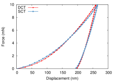
Figure 6: Load-displacement curves for the two steels.

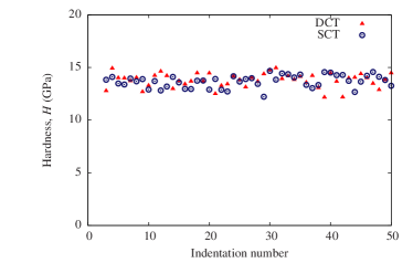
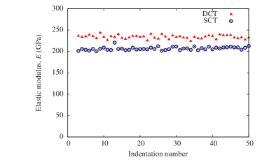
Figure 7: Nanoindentation results. (a) Hardness; (b) Elastic modulus.

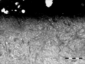
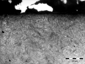
Figure 8: Microstructure of (a) SCT specimen; (b) DCT specimen. Picral etch.

Surface contact fatigue

Compared to conventional oil quenching, both cryogenic treatments lead to a reduction of micropitting (see Fig. 9). Table 6 shows the average area of micropitting measured for each specimen.

Both cryogenic treatments are effective in improving the contact fatigue resistance but due to different effects. Since the precipitation of $\eta$-Fe₂C in the SCT steel is not significant ($4\%$) the improvement is probably due the transformation of retained austenite. On the other hand, the intense precipitation of $\eta$-Fe₂C in the DCT steel ($20\%$) increases the fracture toughness of martensite by a mechanism specific to metal matrix composites: (1) crack deflection by the stiffer nanoparticle, (2) crack trapping by nanoparticle which results in significant reduction of stresses in the matrix and, (3) crack bridging ahead of the main crack tip.

Table 6: Average micropitting area, $M\,(\%)$.

Sample	DCT	SCT	Oil quenched
$M\,(\%)$	$4.2\pm 1.2$	$5.8\pm 1.4$	$8.2\pm 1.5$

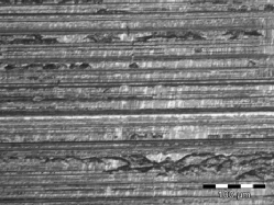
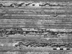
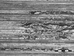
Figure 9: Light microscopy images showing the surface of (a) DCT sample; (b) SCT sample; (c) oil quenched sample.

Conclusions

In this work the elastic properties of $\eta$-Fe₂C have been determined from ab initio calculations. The hardness and elastic modulus of a case carburised gear steel subjected to cryogenic treatments (SCT and DCT) have been determined by nanoindentation. Based on the elastic modulus of $\eta$-Fe₂C derived from first principles the volume fraction of carbides was estimated. It was found that the microstructure of the SCT steel contains only $4\%$ of $\eta$-Fe₂C the microstructure of the DCT steel contains $20\%$ of $\eta$-Fe₂C. The precipitation of eta carbide in the DCT steel results in an increase in elastic modulus but there is no difference in the hardness of the DCT steel and SCT steel.

The micropitting tests carried out under EHL conditions showed that cryogenic treatments improved the surface contact fatigue behaviour of S156 case carburised steel. The average micropitting area was $8.2\%$ for the oil quenched steel, $5.8\%$ for the SCT steel and $4.2\%$ for the DCT steel. Both cryogenic treatments are effective in reducing micropitting but the mechamisms involved are probably different. The improved contact fatigue performance of the SCT steel is due to the transformation of retained austenite while in the DCT steel this is due to an increase in fracture toughness as a result of eta carbide precipitation. The nano-carbides act as reinforcements in the martensite matrix by one of the mechanisms specific to composite materials: (1) crack deflection, (2) crack trapping and, (3) crack bridging.

- (1) Y. Nakamura, S. Nagakura, Transactions of the Japan Institute of Metals 27(11), 842 (1986)
- (2) P. Baldissera, C. Delprete, The Open Mechanical Engineering Journal (2), 1 (2008)
- (3) A. Bensely, A. Prabhakaran, D. Mohan Lal, G. Nagarajan, Cryogenics 45(12), 747 (2006). DOI 10.1016/j.cryogenics.2005.10.004
- (4) D. Das, A. Dutta, K. Ray, Wear 267(9-10), 1371 (2009). DOI 10.1016/j.wear.2008.12.051
- (5) D. Das, A.K. Dutta, K.K. Ray, Materials Science and Engineering A 527(9), 2182 (2010). DOI 10.1016/j.msea.2009.10.070
- (6) D. Das, A.K. Dutta, K.K. Ray, Materials Science and Engineering A 527(9), 2194 (2010). DOI 10.1016/j.msea.2009.10.071
- (7) V. Firouzdor, E. Nejati, F. Khomamizadeh, Journal of Materials Processing Technology 206(1-3), 467 (2008). DOI 10.1016/j.jmatprotec.2007.12.072
- (8) A. Molinari, M. Pellizzari, S. Gialanella, G. Straffelini, K. Stiasny, (2001), vol. 118, pp. 350–355. DOI 10.1016/S0924-0136(01)00973-6
- (9) P. Baldissera, Materials and Design 30(9), 3636 (2009). DOI 10.1016/j.matdes.2009.02.019
- (10) P. Baldissera, C. Delprete, Materials and Design 30(5), 1435 (2009). DOI 10.1016/j.matdes.2008.08.015
- (11) A. Bensely, D. Senthilkumar, D. Mohan Lal, G. Nagarajan, A. Rajadurai, Materials Characterization 58(5), 485 (2007). DOI 10.1016/j.matchar.2006.06.019
- (12) A. Bensely, S. Venkatesh, D. Mohan Lal, G. Nagarajan, A. Rajadurai, K. Junik, Materials Science and Engineering A 479(1-2), 229 (2008). DOI 10.1016/j.msea.2007.07.035
- (13) A. Bensely, L. Shyamala, S. Harish, D. Mohan Lal, G. Nagarajan, K. Junik, A. Rajadurai, Materials and Design 30(8), 2955 (2009). DOI 10.1016/j.matdes.2009.01.003
- (14) A. Bensely, D. Senthilkumar, S. Harish, D. Mohan Lal, G. Nagarajan, A. Rajadurai, P. Paulin, Gear Solutions pp. 37–51 (2011)
- (15) V. Manoj, K. Gopinath, G. Muthuveerappan, International Symposium of Research Students on Material Science and Engineering pp. 1–11 (2004)
- (16) P. Paulin, Gear Technology 10(2), 26 (1993)
- (17) M. Preciado, P. Bravo, J. Alegre, Journal of Materials Processing Technology 176(1-3), 41 (2006). DOI 10.1016/j.jmatprotec.2006.01.011
- (18) P. Stratton, M. Graf, Cryogenics 49(7), 346 (2009). DOI 10.1016/j.cryogenics.2009.03.007
- (19) A. Oila, Micropitting and Related Phenomena in Case Carburised Gears. Ph.D. thesis, Newcastle University (2003)
- (20) F. Meng, K. Tagashira, R. Azuma, H. Sohma, ISIJ International 34(2), 205 (1994)
- (21) A. Oila, S. Bull, Computational Materials Science 45(2), 235 (2009). DOI 10.1016/j.commatsci.2008.09.013
- (22) C.K. Ande, M.H. Sluiter, Metallurgical and Materials Transactions A 43A, 4436 (2012). DOI 10.1007/s11661-012-1229-y
- (23) L.L. Bao, C.F. Huo, C.M. Deng, Y.W. Li, Ranliao Huaxue Xuebao/Journal of Fuel Chemistry and Technology 37(1), 104 (2009)
- (24) H. Faraoun, Y. Zhang, C. Esling, H. Aourag, Journal of Applied Physics 99(9), 093508 (2006). DOI 10.1063/1.2194118
- (25) Z. Lv, S. Sun, P. Jiang, B. Wang, W. Fu, Computational Materials Science 42(4), 692 (2008). DOI 10.1016/j.commatsci.2007.10.007
- (26) R. Hill, Physical Society – Proceedings 65(389A), 349 (1952)
- (27) M. Dirand, L. Afqir, Acta Metallurgica 31(7), 1089 (1983). DOI 10.1016/0001-6160(83)90205-5
- (28) Y. Hirotsu, S. Nagakura, Acta Metallurgica 20(4), 645 (1972)
- (29) S. Nagakura, Y. Hirotsu, M. Kusunoki, T. Suzuki, Y. Nakamura, Metallurgical Transactions. A, Physical metallurgy and materials science 14A(6), 1025 (1981)
- (30) J.P. Perdew, K. Burke, M. Ernzerhof, Phys. Rev. Lett. 77, 3865 (1996). DOI 10.1103/PhysRevLett.77.3865
- (31) P. Giannozzi, S. Baroni, N. Bonini, M. Calandra, R. Car, C. Cavazzoni, D. Ceresoli, G.L. Chiarotti, M. Cococcioni, I. Dabo, A. Dal Corso, S. De Gironcoli, S. Fabris, G. Fratesi, R. Gebauer, U. Gerstmann, C. Gougoussis, A. Kokalj, M. Lazzeri, L. Martin-Samos, N. Marzari, F. Mauri, R. Mazzarello, S. Paolini, A. Pasquarello, L. Paulatto, C. Sbraccia, S. Scandolo, G. Sclauzero, A.P. Seitsonen, A. Smogunov, P. Umari, R.M. Wentzcovitch, Journal of Physics Condensed Matter 21(39), 395502 (2009). DOI 10.1088/0953-8984/21/39/395502
- (32) K. Laasonen, A. Pasquarello, R. Car, C. Lee, D. Vanderbilt, Phys. Rev. B 47, 10142 (1993). DOI 10.1103/PhysRevB.47.10142
- (33) P. Hohenberg, W. Kohn, Phys. Rev. 136, B864 (1964). DOI 10.1103/PhysRev.136.B864
- (34) W. Kohn, L.J. Sham, Phys. Rev. 140, A1133 (1965). DOI 10.1103/PhysRev.140.A1133
- (35) C. Jiang, S. Srinivasan, A. Caro, S. Maloy, Journal of Applied Physics 103(4), 043502 (2008). DOI 10.1063/1.2884529
- (36) H.J. Monkhorst, J.D. Pack, Phys. Rev. B 13, 5188 (1976). DOI 10.1103/PhysRevB.13.5188
- (37) N. Marzari, D. Vanderbilt, A. De Vita, M.C. Payne, Phys. Rev. Lett. 82, 3296 (1999). DOI 10.1103/PhysRevLett.82.3296
- (38) F. Murnaghan, Proc Natl Acad Sci U. S. A. 30(9), 244 (1944)
- (39) A. Reuss, Zeitschrift für Angewandte Mathematik und Mechanik 9(1), 49 (1929)
- (40) W. Voigt, Königliche Gesellschaft der Wissenschaften zu Göttingen 34(3–100) (1887)
- (41) W. Oliver, G. Pharr, Journal of Materials Research 7(6), 1564 (1992)
- (42) A. Oila, S. Bull, Wear 258(10), 1510 (2005). DOI 10.1016/j.wear.2004.10.012