Josephson physics of spin-orbit coupled elongated Bose-Einstein condensates

Abstract

We consider an ultracold bosonic binary mixture confined in a one-dimensional double-well trap. The two bosonic components are assumed to be two hyperfine internal states of the same atom. We suppose that these two components are spin-orbit coupled between each other. We employ the two-mode approximation starting from two coupled Gross-Pitaevskii equations and derive a system of ordinary differential equations governing the temporal evolution of the inter-well population imbalance of each component and that between the two bosonic species. We study the Josephson oscillations of these spin-orbit coupled Bose-Einstein condensates by analyzing the interplay between the interatomic interactions and the spin-orbit coupling and the self-trapped dynamics of the inter-species imbalance. We show that the dynamics of this latter variable is crucially determined by the relationship between the spin-orbit coupling, the tunneling energy, and the interactions.

I Introduction

In the last few years artificial spin-orbit (SO) coupling has been realized in the laboratory with both neutral bosonic systems so-bose1 and fermionic atomic gases so-fermi1 ; so-fermi2 . These achievements have stimulated theoretical efforts to understand the role of the SO with Rashba rashba and Dresselhaus dresselhaus terms in the physics of the ultracold atoms.

Spin-orbit coupled Bose-Einstein condensates (BECs) have been considered in Refs. stringari1 ; stringari2 , where the authors have determined the zero-temperature phase diagram and studied the excitation spectrum in uniform systems. Bosons in two SO coupled hyperfine states have been investigated in different contexts, for instance by exploring different confinements and geometries, e.g. two-dimensional (2D) periodic geometries cole , tight 2D harmonic potential plus a generic one-dimensional (1D) loose potential salasnich1 , and confinements in quasi 1D parabolic trap achilleos . Also the richer strongly correlated quantum Hall phases stemming from the spin-orbit coupling (which can be regarded as a non-abelian external field) have been recently discussed tb10 ; tob13 . On the fermionic side, the experimental realization of the SO coupling has produced a growing interest in the study of its role in the crossover from the Bardeen-Cooper-Schrieffer state of weakly bound Fermi pairs to the BEC of molecular dimers both for a three-dimensional (3D) uniform Fermi gas bcs3d ; dms ; zhou2 and in the 2D case bcs2d ; dms ; zhou2 .

One of the richest scenarios opens up when two internal hyperfine states of the same bosonic atom are coupled between each other by means of two counter-propagating laser beams and confined by a one-dimensional double-well. This framework represents the ideal arena to analyze the atomic counterpart of the Josephson effect which occurs in the superconductor-oxide-superconductor junctions book-barone with bosonic binary mixtures lobo ; xu ; satja ; diaz1 ; ajj1 ; ajj2 ; rabijosephson ; brunonjp . It is worth noting that Josephson physics with bosonic mixtures seems within reach for a number of experimental groups which have in the last years studied single component Josephson physics Albiez05 ; GO07 ; esteve08 ; gross10 ; treut10 ; zib10 ; amo13 ; berrada13 .

The aim of the present work is to study the Josephson oscillations with SO coupled Bose-Einstein condensates. In this case, the boson-dynamics is ruled by two coupled 3D Gross-Pitaevskii equations, the couplings consisting in the intra- and inter-species interactions and spin-orbit. By employing the two-spatial mode approximation milburn ; smerzi , neglecting the interatomic interactions between bosons in different wells, and assuming that the Rashba and the Dresselhaus velocities are equal, one derives a system of ordinary differential equations (ODEs). The solution of these ODEs provides the temporal evolution of the relevant variables of the problem. These are the two fractional population imbalances, $z_{k}$, defined as the difference in the occupation of the two wells for each bosonic component labeled by $k=1,2$. On top of these we define the total population imbalance, $z_{12}$, between the bosons in species $1$ and those in species $2$. We term this latter variable the polarization, i.e. zero polarization implies an equal amount of atoms populating the components $1$ and $2$, while the system is fully polarized if all atoms populate either of the two species. The dynamical evolution of $z_{12}$ gives the interchange of atoms between the two bosonic components and is therefore directly related to the SO coupling.

The issue of the Josephson physics in the presence of spin-orbit has been recently addressed by Zhang and co-workers zhang that (as we comment in Sec.  II) have analyzed the problem starting from a quantum single-particle (SP) Hamiltonian different from that we consider in this paper. The Hamiltonian that will used here - to make stronger the link with experiments on SO coupled BECs - is the same considered by Lin et al. so-bose1 .

We numerically solve the aforementioned ODEs and study the temporal behavior of the three $z$’s and their corresponding canonically conjugated phases. We focus on the interplay between the boson-boson interaction and the inter-well spin-orbit coupling (the intra-well SO is zero in first approximation) in determining the importance of the interchange of atoms between the two bosonic species on the two canonical effects: self-trapping and macroscopic tunneling phenomena. In particular, we point out that an analogous of the macroscopic quantum self-trapping that one observes for the variable $z_{k}$ satja ; ajj2 exists for the polarization $z_{12}$ as well. During the $z_{12}$ self-trapped dynamics, on the average, one bosonic component is more populated than the other one.

The article is organized in the following way. First, in Sec. II we describe the single particle Hamiltonian of the system, following the experimental realization of Ref. so-bose1 . In Sec. III we present the mean-field description of the problem. In Sec. IV two-mode approximation is exploited to derive the ordinary differential equations that we use to describe the dynamics of our system. In Sec. V we study the effect of the spin-orbit term on the macroscopic quantum tunneling and self-trapping. A summary and conclusions are provided in Sec. VI.

II Artificial spin-orbit coupling

We consider two counter-propagating laser beams which couple two internal hyperfine states of the same bosonic atom (e.g., the $m_{F}=0,1$ components of an ⁸⁷Rb $F=1$ spinor condensate as in the experiment carried out by Lin and co-workers so-bose1 ) by a resonant stimulated two-photon Raman transition characterized by a Rabi frequency $\Omega_{R}$. This transition can be induced by a laser beam with a detuning $\delta$ with respect to the spacing between the energy levels of the two hyperfine states. The two internal hyperfine states define the pseudo-spin space of each atom. The single-particle (SP) quantum Hamiltonian can be written as

$$H_{sp} = \left[{{\bf p}^{2}\over 2m}+U({\bf r})\right]\sigma_{0}+v_{R}\left(p_{x}\sigma_{y}-p_{y}\sigma_{x}\right)$$ (1)

$$+ v_{D}\left(p_{x}\sigma_{y}+p_{y}\sigma_{x}\right)+{\hbar\Omega_{R}\over 2}\sigma_{z}+{\hbar\delta\over 2}\sigma_{y}\;,$$

where ${\bf p}=(p_{x},p_{y},p_{z})=-i\hbar(\partial_{x},\partial_{y},\partial_{z})$ is the linear momentum operator, $U({\bf r})$ is the external trapping potential, $v_{R}$ and $v_{D}$ are, respectively, the Rashba and Dresselhaus velocities, $\sigma_{0}$ is the $2\times 2$ identity matrix, and $\sigma_{x}$, $\sigma_{y}$, $\sigma_{z}$ are the Pauli matrices. In the recent experiments so-bose1 ; so-fermi1 ; so-fermi2 one has $v_{R}=v_{D}\equiv v$, which is the configuration that we shall consider in the present paper. In this configuration, the terms proportional to the Pauli matrices in the single-particle Hamiltonian (1) are the same appearing in Eq. (2) of zhang , provided to perform on the SP Hamiltonian of Zhang and co-workers the following global pseudo-spin rotation: $\sigma_{z}\rightarrow\sigma_{y}$, $\sigma_{y}\rightarrow\sigma_{x}$, and $\sigma_{x}\rightarrow\sigma_{z}$.

III Mean-field description: Gross-Pitaevskii equations

We consider a dilute binary condensate with a spin-orbit coupling term as described above, whose single-particle Hamiltonian is given by Eq. (1). The ultracold atomic cloud is further assumed to be confined in the transverse $(y,z)$ plane by a strong harmonic potential with frequency $\omega_{\bot}$ and in the axial ($x$) direction by a generic weak potential $V(x)$, namely

$$U(\mathbf{r})=V(x)+{1\over 2}m\omega_{\bot}^{2}(y^{2}+z^{2})\;.$$ (2)

Under the hypothesis that the boson-boson interactions (intra- and inter-species) can be described by a contact potential, the two time-dependent 3D Gross-Pitaevskii equations (GPEs) which describe the binary condensate are

$$i\,\partial_{t}\psi_{1}=\Big{[}-{\frac{1}{2}}\nabla^{2}+V(x)+{\frac{1}{2}}(y^{2}+z^{2})+\Gamma+2\pi\,\tilde{g}_{1}|\psi_{1}|^{2}$$

$$+2\pi\,\tilde{g}_{12}|\psi_{2}|^{2}\Big{]}\psi_{1}-(\gamma\partial_{x}+i\tilde{\delta})\psi_{2}\;,$$ (3)

$$i\,\partial_{t}\psi_{2}=\Big{[}-{\frac{1}{2}}\nabla^{2}+V(x)+{\frac{1}{2}}(y^{2}+z^{2})-\Gamma+2\pi\,\tilde{g}_{2}|\psi_{2}|^{2}$$

$$+2\pi\,\tilde{g}_{12}|\psi_{1}|^{2}\Big{]}\psi_{2}+(\gamma\partial_{x}+i\tilde{\delta})\psi_{1}\;,$$ (4)

where lengths, times, and energies are written in units of $a_{\bot}=\sqrt{\hbar/(m\omega_{\bot})}$, $\omega_{\bot}^{-1}$, and $\hbar\omega_{\bot}$, respectively. Here $\psi_{k}(x,y,z,t)$ is the macroscopic wave function of the $k$th atomic hyperfine state ($k=1,2$). The number of atoms populating each hyperfine state can be computed at any time as

$$\int\int\int\left|\psi_{k}(x,y,z,t)\right|^{2}dx\ dy\ dz=N_{k}(t)\;.$$ (5)

The strengths of the intra- and inter-species interactions are given by

$$\tilde{g}_{k}\equiv 2a_{k}/a_{\bot},~{}\tilde{g}_{12}\equiv 2a_{12}/a_{\bot},$$ (6)

where $a_{k}$ and $a_{12}$ are the $s$-wave scattering lengths pertaining, respectively, to the intra-species interaction and inter-species one.

Note that $\gamma=2v/(a_{\bot}\omega_{\bot})$ is the dimensionless SO coupling, $\Gamma=\Omega_{R}/(2\omega_{\bot})$ and $\tilde{\delta}=\delta/(2\omega_{\bot})$ are the dimensionless Rabi and detuning frequencies, respectively.

These GPEs can be derived with the ordinary variational procedure from the Lagrangian density

$$L=L_{0}+L_{SO}+L_{I}\;,$$ (7)

where

$$L_{0}=\sum_{k=1,2}\psi_{k}^{\ast}\left[i\,\partial_{t}+{\frac{1}{2}}\nabla^{2}-V(x)-{\frac{1}{2}}(y^{2}+z^{2})\right]\psi_{k}\;$$ (8)

is the Lagrangian density of the non-interacting binary condensate,

$$L_{SO} = -\Gamma\left(|\psi_{1}|^{2}-|\psi_{2}|^{2}\right)+\gamma\Big{(}\psi_{1}^{*}\partial_{x}\psi_{2}-\psi_{2}^{*}\partial_{x}\psi_{1}\Big{)}$$ (9)

$$+ i\tilde{\delta}\Big{(}\psi_{1}^{*}\psi_{2}-\psi_{2}^{*}\psi_{1}\Big{)}\;$$

is the SO coupling contribution, and

$$L_{I}=-{\pi\,\tilde{g}_{1}}|\psi_{1}|^{4}-{\pi\,\tilde{g}_{2}}|\psi_{2}|^{4}-2\pi\,\tilde{g}_{12}|\psi_{1}|^{2}|\psi_{2}|^{2}\;,$$ (10)

is the term due to $s$-wave interactions between the bosonic atoms.

By assuming a strongly localized cloud in the transverse plane and weakly localized in the axial direction (see the above discussion about the trapping potential (2)), we can derive a system of effective one-dimensional Gross-Pitaevskii equations by adopting the usual Gaussian ansatz for the wave functions $\psi_{k}$ ($k=1,2$) in the directions $y$ and $z$, that is

$$\psi_{k}(x,y,z,t)={\frac{1}{\sqrt{\pi}a_{\bot}}}\exp{\left\{-{\frac{y^{2}+z^{2}}{2a_{\bot}^{2}}}\right\}}\,f_{k}(x,t)\;,$$ (11)

where the complex functions $f_{k}(x,t)$ ($k=1,2$) are dynamical fields, obeying normalization $\int_{-\infty}^{+\infty}\left|f_{k}(x,t)\right|^{2}dx=N_{k}$, as it follows from Eqs. (5) and (11).

By inserting the ansatz (11) in the Lagrangian density $L$ given by Eq. (7) (its contributions being the right-hand sides of Eqs. (8)-(10)) and performing the integration in the transverse directions ($y$ and $z$) starting from $\displaystyle{\int dxdydzL}$ we obtain the effective 1D Lagrangian

$$\bar{L} = \int\,dx\bigg{(}\bigg{[}\sum_{k=1,2}f_{k}^{*}(i\partial_{t}+\frac{1}{2}\partial_{x}^{2})f_{k}$$ (12)

$$- (1+V(x))|f_{k}|^{2}-\frac{\tilde{g}_{k}}{2}|f_{k}|^{4}\bigg{]}-\tilde{g}_{12}\,|f_{1}|^{2}|f_{2}|^{2}$$

$$- \Gamma(|f_{1}|^{2}-|f_{2}|^{2})+\gamma\,(f_{1}^{*}\partial_{x}f_{2}-f_{2}^{*}\partial_{x}f_{1})$$

$$+ i\tilde{\delta}(f_{1}^{*}f_{2}-f_{2}^{*}f_{1})\bigg{)}\;.$$

By varying $\bar{L}$ with respect to $f_{k}^{*}$ we get the following system formed by two coupled 1D GPEs

$$i\,\partial_{t}f_{1} = \Big{[}-{\frac{1}{2}}\partial_{x}^{2}+V(x)+\Gamma+\tilde{g}_{1}|f_{1}|^{2}+\tilde{g}_{12}|f_{2}|^{2}\Big{]}f_{1}$$ (13)

$$- (\gamma\partial_{x}+i\tilde{\delta})\,f_{2}\;,$$

$$i\,\partial_{t}f_{2} = \Big{[}-{\frac{1}{2}}\partial_{x}^{2}+V(x)-\Gamma+\tilde{g}_{2}|f_{2}|^{2}+\tilde{g}_{12}|f_{1}|^{2}\Big{]}f_{2}$$ (14)

$$+ (\gamma\partial_{x}+i\tilde{\delta})\,f_{1}\;.$$

IV Bimodal approximation

Let us suppose that the potential $V(x)$ at the right-hand side of Eq. (2) is a symmetric double-well potential $V_{\mathrm{DW}}(x)$. To describe the dynamics by a finite-mode approximation, we use a two-mode ansatz for each wave function $f_{k}$ (recall $k=1,2$), as originally introduced in milburn :

$$f_{k}(x,t)=\Psi_{k}^{L}(t)\phi_{k}^{L}(x)+\Psi_{k}^{R}(t)\phi_{k}^{R}(x)\;.$$ (15)

The functions $\phi_{k}^{\alpha}(x)$ ($\alpha=L,R$) - that we consider as real functions as done for example in ajj1 ; ajj2 ; rabijosephson - are single particle wave functions tightly localized in the $\alpha$th well, while the time dependence is encoded in $\Psi_{k}^{\alpha}(t)\equiv\sqrt{N_{k}^{\alpha}(t)}\ e^{i\theta_{k}^{\alpha}(t)}\;,$ where the total number of particles in the $k$th species is given by $N_{k}^{L}(t)+N_{k}^{R}(t)=\left|\Psi_{k}^{L}(t)\right|^{2}+\left|\Psi_{k}^{R}(t)\right|^{2}\equiv N_{k}(t)$. The functions $\phi_{k}^{\alpha}(x)$ satisfy the following orthonormalization conditions: $\int dx(\phi_{k}^{\alpha}(x))^{2}=1$ and $\int dx\phi_{k}^{L}(x)\phi_{k}^{R}(x)=0$.

At this point, we exploit the two-mode approximation for $f_{k}(x,t)$ given by Eq. (15) in each of the two coupled one-dimensional Gross-Pitaevskii equations, (13) and (14). By left-multiplying both the left-hand side and the right-hand one of the $f_{k}$-1D GPE for $\phi_{k}^{\alpha}(x)$ and integrating in the $x$ direction, one obtains the equations of motion for $N_{k}^{\alpha}$ and $\theta_{k}^{\alpha}$ (note that here one has to take into account the above orthonormalization conditions). We retain only the integrals with wave functions localized in the same well for the boson-boson interactions and terms related to the Rabi and detuning terms. Conversely, due to the derivative coupling, both the SO coupling in the same and different wells have to be considered. The equations of motion for $N_{k}^{\alpha}$ and $\theta_{k}^{\alpha}$ thus read,

$$\dot{N}_{k}^{\alpha} = -2J_{k}\sqrt{N_{k}^{\alpha^{\prime}}N_{k}^{\alpha}}\sin\left(\theta_{k}^{\alpha^{\prime}}-\theta_{k}^{\alpha}\right)$$ (16)

$$+ 2S_{12}^{\alpha}\sqrt{N_{3-k}^{\alpha}N_{k}^{\alpha}}\sin\left(\theta_{k}^{\alpha}-\theta_{3-k}^{\alpha}\right)$$

$$\pm 2\bar{S}_{12}^{\alpha,\alpha^{\prime}}\sqrt{N_{3-k}^{\alpha^{\prime}}N_{k}^{\alpha}}\sin\left(\theta_{k}^{\alpha}-\theta_{3-k}^{\alpha^{\prime}}\right)$$

$$\mp 2D_{12}^{\alpha}\sqrt{N_{3-k}^{\alpha}N_{k}^{\alpha}}\cos\left(\theta_{k}^{\alpha}-\theta_{3-k}^{\alpha}\right)\;,$$

$$\dot{\theta}_{k}^{\alpha} = -\left(U_{k}N_{k}^{\alpha}+\epsilon_{k}+U_{12}N_{3-k}^{\alpha}\pm\Gamma\right)$$ (17)

$$+ J_{k}\sqrt{\frac{N_{k}^{\alpha^{\prime}}}{N_{k}^{\alpha}}}\cos\left(\theta_{k}^{\alpha}-\theta_{k}^{\alpha^{\prime}}\right)$$

$$+ S_{12}^{\alpha}\sqrt{\frac{N_{3-k}^{\alpha}}{N_{k}^{\alpha}}}\cos\left(\theta_{k}^{\alpha}-\theta_{3-k}^{\alpha}\right)$$

$$\pm \bar{S}_{12}^{\alpha,\alpha^{\prime}}\sqrt{\frac{N_{3-k}^{\alpha^{\prime}}}{N_{k}^{\alpha}}}\cos\left(\theta_{k}^{\alpha}-\theta_{3-k}^{\alpha^{\prime}}\right)$$

$$\pm D_{12}^{\alpha}\sqrt{\frac{N_{3-k}^{\alpha}}{N_{k}^{\alpha}}}\sin\left(\theta_{k}^{\alpha}-\theta_{3-k}^{\alpha}\right).$$

The sign in front of the $D_{12}$ term in Eq. (16) is minus (plus) for $k=1(2)$. In Eq. (17) the sign in front of $\Gamma$ is plus (minus) for $k=1(2)$. In both equations the sign $+$ in front of $\bar{S}_{12}^{\alpha,\alpha^{\prime}}$ is plus (minus) for the component 1(2).

The following constants are introduced in terms of the single-particle functions $\phi_{k}^{\alpha}$:

$$\epsilon_{k}^{\alpha}=\int dx\,\bigg{[}\phi_{k}^{\alpha}(x)\,\big{(}-\frac{1}{2}\partial^{2}_{x}+V_{\mathrm{DW}}(x)\big{)}\,\phi_{k}^{\alpha}(x)\bigg{]}+1,$$

$$U_{k}=\tilde{g}_{k}\int dx\,(\phi_{k}^{\alpha})^{4},$$

$$J_{k}=-\int dx\,\bigg{[}\phi_{k}^{L}(x)\,\big{(}-\frac{1}{2}\partial^{2}_{x}+V_{\mathrm{DW}}(x)\big{)}\,\phi_{k}^{R}(x)\bigg{]},$$

$$U_{12}=\tilde{g}_{12}\int dx\,(\phi_{1}^{\alpha})^{2}(\phi_{2}^{\alpha})^{2},$$

$$S_{12}^{\alpha}=\gamma\,\int dx\,\phi_{1}^{\alpha}(x)\partial_{x}\phi_{2}^{\alpha}(x)\;,$$

$$\bar{S}_{12}^{\alpha,\alpha^{\prime}}=\gamma\,\int dx\,\phi_{1}^{\alpha}(x)\partial_{x}\phi_{2}^{\alpha^{\prime}}(x)\;,$$

$$D_{12}^{\alpha}=\tilde{\delta}\int dx\,\phi_{1}^{\alpha}(x)\phi_{2}^{\alpha}(x).$$ (18)

In obtaining the equations of motion (16) and (17), we have used the double-well left-right symmetry so that: $\epsilon_{k}^{L}=\epsilon_{k}^{R}\equiv\epsilon_{k}$, $U_{k}^{L}=U_{k}^{R}\equiv U_{k}$ and $U_{12}^{L}=U_{12}^{R}\equiv U_{12}$. We have employed, moreover, the following properties: by integrating by parts we have both $S_{12}^{\alpha}=-S_{21}^{\alpha}$ and $\bar{S}_{12}^{\alpha,\alpha^{\prime}}=-\bar{S}_{21}^{\alpha^{\prime},\alpha}$, and finally that $\bar{S}_{12}^{\alpha,\alpha^{\prime}}=-\bar{S}_{12}^{\alpha^{\prime},\alpha}$.

We are assuming that $m_{1}=m_{2}=m$, thus it is possible to work with the same localized modes for both components, that is $\phi_{1}^{\alpha}=\phi_{2}^{\alpha}=\phi^{\alpha}$ ($\alpha=L,R$). If this is the case, $\epsilon_{1}=\epsilon_{2}=\epsilon$, $J_{1}=J_{2}=J$, and $D_{12}=\tilde{\delta}$. This also implies that $S_{12}^{\alpha}$ and $S_{21}^{\alpha}$ vanish. After defining $S_{+}=\bar{S}_{12}^{L,R}=-\bar{S}_{21}^{R,L}$ and $S_{-}=\bar{S}_{12}^{R,L}=-\bar{S}_{21}^{L,R}$, we can rewrite the equations of motion (16) and (17) as:

$$\dot{N}_{k}^{\alpha} = -2J\sqrt{N_{k}^{\alpha^{\prime}}N_{k}^{\alpha}}\sin\left(\theta_{k}^{\alpha^{\prime}}-\theta_{k}^{\alpha}\right)$$ (19)

$$+ 2S_{\pm(\mp)}\sqrt{N_{3-k}^{R(L)}N_{k}^{L(R)}}\sin\left(\theta_{k}^{L(R)}-\theta_{3-k}^{R(L)}\right)$$

$$\mp 2\tilde{\delta}\sqrt{N_{3-k}^{\alpha}N_{k}^{\alpha}}\cos\left(\theta_{k}^{\alpha}-\theta_{3-k}^{\alpha}\right)\;,$$

$$\dot{\theta}_{k}^{\alpha} = -\left(U_{k}N_{k}^{\alpha}+U_{12}N_{3-k}^{\alpha}\pm\Gamma\right)$$ (20)

$$+ J\sqrt{\frac{N_{k}^{\alpha^{\prime}}}{N_{k}^{\alpha}}}\cos\left(\theta_{k}^{\alpha}-\theta_{k}^{\alpha^{\prime}}\right)$$

$$+ S_{\pm(\mp)}\sqrt{\frac{N_{3-k}^{R(L)}}{N_{k}^{L(R)}}}\cos\left(\theta_{k}^{L(R)}-\theta_{3-k}^{R(L)}\right)$$

$$\pm \tilde{\delta}\sqrt{\frac{N_{3-k}^{\alpha}}{N_{k}^{\alpha}}}\sin\left(\theta_{k}^{\alpha}-\theta_{3-k}^{\alpha}\right).$$

The upper (lower) sign in these equations holds for $k=1(2)$. For the SO coupling term ($S_{\pm}$), the symbol without (with) parenthesis holds for the equation of motion of the occupation $N_{k}^{\alpha}$ or $\theta_{k}^{\alpha}$ with $\alpha=L(R)$. In Appendix A we show how to derive these equations as the semiclassical limit of the exact bimodal many-body Hamiltonian. Note that the equations (19) and (20) can be regarded as obtained from a classical Hamiltonian, hence being $\theta_{k}^{\alpha}$ and $N_{k}^{\alpha}$ the canonical conjugate variables. Then, $\dot{N}_{k}^{\alpha}=\partial H/\partial\theta_{k}^{\alpha}$ and $\dot{\theta}_{k}^{\alpha}=-\partial H/\partial N_{k}^{\alpha}$ with a classical Hamiltonian:

$$H = \sum_{k,\alpha}\left\{\left[\frac{1}{2}U_{k}N_{k}^{\alpha}\pm\Gamma+\frac{1}{2}U_{12}N_{3-k}^{\alpha}\right]N_{k}^{\alpha}\right.$$ (21)

$$- \left.J\sqrt{N_{k}^{\alpha}N_{k}^{\alpha^{\prime}}}\cos\left(\theta_{k}^{\alpha}-\theta_{k}^{\alpha^{\prime}}\right)\right\}$$

$$- 2S_{+}\sqrt{N_{2}^{R}N_{1}^{L}}\cos\left(\theta_{1}^{L}-\theta_{2}^{R}\right)$$

$$- 2S_{-}\sqrt{N_{2}^{L}N_{1}^{R}}\cos\left(\theta_{1}^{R}-\theta_{2}^{L}\right)$$

$$- 2\sum_{\alpha}\left\{\tilde{\delta}\sqrt{N_{1}^{\alpha}N_{2}^{\alpha}}\sin\left(\theta_{1}^{\alpha}-\theta_{2}^{\alpha}\right)\right\},$$

with the upper (lower) sign for $k=1(2)$. Noting that since there is one constant of motion, that is the total number of atoms, we can reduce the number of variables through the following transformation:

$$\left(\begin{array}[]{c}1\\ z_{1}\\ z_{2}\\ z_{12}\end{array}\right)\!=\!\frac{\mathrm{M}}{N}\left(\begin{array}[]{c}N_{1}^{L}\\ N_{1}^{R}\\ N_{2}^{L}\\ N_{2}^{R}\end{array}\right)\!,\,\,\left(\begin{array}[]{c}\theta_{N}\\ \theta_{1}\\ \theta_{2}\\ \theta_{12}\end{array}\right)\!=\!-\mathrm{M}\left(\begin{array}[]{c}\theta_{1}^{L}\\ \theta_{1}^{R}\\ \theta_{2}^{L}\\ \theta_{2}^{R}\end{array}\right),$$ (22)

with

$$\mathrm{M}=\left(\begin{array}[]{cccc}1&1&1&1\\ 1&-1&0&0\\ 0&0&1&-1\\ 1&1&-1&-1\end{array}\right).$$

The set of new variables $\{z_{i},\theta_{i}\}$ are also canonically conjugate because their Poisson brackets fulfill

$$\{z_{i},\theta_{j}\}\equiv\sum_{k,\alpha}\left(\frac{\partial z_{i}}{\partial N_{k}^{\alpha}}\frac{\partial\theta_{j}}{\partial\theta_{k}^{\alpha}}-\frac{\partial z_{i}}{\partial\theta_{k}^{\alpha}}\frac{\partial\theta_{j}}{\partial N_{k}^{\alpha}}\right)=\delta_{ij}.$$ (23)

From the transformations (22), one realizes that

$$z_{1}=\frac{N_{1}^{L}-N_{1}^{R}}{N}\;,z_{2}=\frac{N_{2}^{L}-N_{2}^{R}}{N}$$

$$z_{12}=\frac{N_{1}-N_{2}}{N}\;,$$ (24)

with $N_{k}=N_{k}^{L}+N_{k}^{R}$. The phases associated to the $z_{1}$, $z_{2}$, and $z_{12}$ are, respectively

$$\theta_{1}=\theta_{1}^{R}-\theta_{1}^{L}\;,\theta_{2}=\theta_{2}^{R}-\theta_{2}^{L}$$

$$\theta_{12}=\theta_{2}^{L}+\theta_{2}^{R}-(\theta_{1}^{L}+\theta_{1}^{R})\;.$$ (25)

In the rotated frame zhang , $N_{\uparrow}$ and $N_{\downarrow}$, the numbers of bosons in the dressed hyperfine states $\uparrow$ and $\downarrow$, can be written in terms of our quantities as follows

$$N_{\sigma}=\frac{1}{2}\big{(}N_{1}+N_{2}\pm 2\,\sum_{\alpha=L,R}\sqrt{N_{1}^{\alpha}N_{2}^{\alpha}}\cos(\theta_{1}^{\alpha}-\theta_{2}^{\alpha})\big{)}$$ (26)

with plus (minus) for $\sigma=\uparrow(\downarrow)$, and $N_{k}^{\alpha}$ and $\theta_{k}^{\alpha}$ solutions of Eqs. (19)-(20). Accordingly, the population imbalance $z_{\uparrow,\downarrow}=(N_{\uparrow}-N_{\downarrow})/N$ is related to our variables in the following way:

$$z_{\uparrow,\downarrow}=\frac{2\big{(}\sum_{\alpha=L,R}\sqrt{N_{1}^{\alpha}N_{2}^{\alpha}}\cos(\theta_{1}^{\alpha}-\theta_{2}^{\alpha})\big{)}}{N}\;.$$ (27)

Remarkably, the variables (IV) and (IV) are directly related to the usual Josephson physics. Namely, $z_{k}$ is the population imbalance of component $k$, $\theta_{k}$ is its corresponding canonical phase. The polarization $z_{12}$ measures the total population transfer between both components, that is, the population imbalance between the first and the second species. In the absence of spin-orbit coupling the variable $z_{12}$ becomes a constant of motion. Its evolution will thus be intimately related to the effect of the SO term. $\theta_{12}$ is the canonical phase associated to $z_{12}$.

In terms of these new variables the Hamiltonian governing the dynamics is $H^{\prime}=2H/N$ which reads

$$H^{\prime}\!\! \!=\! \!2\Gamma z_{12}-\!2J\sum_{k}\sqrt{(z_{12}\!\pm\!1)^{2}\!-\!4z_{k}^{2}}\cos\left(\theta_{k}\right)$$

$$\!+\!\! \!\!\frac{1}{8}N\sum_{k}U_{k}\left[(z_{12}\!\pm\!1)^{2}\!+\!4z_{k}^{2}\right]\!+\!\frac{1}{4}U_{12}N(1\!+\!4z_{1}z_{2}\!-\!z_{12}^{2})$$

$$\!+\!\! \!\!2S_{+}\!\left[\left(1\!-\!2z_{2}\!-\!z_{12}\right)\!\left(1\!+\!2z_{1}\!+\!z_{12}\right)\right]^{\frac{1}{2}}\!\cos[\frac{1}{2}(\theta_{1}\!+\!\theta_{2}\!+\!\theta_{12})]$$

$$\!+\!\! \!\!2S_{-}\!\left[\left(1\!+\!2z_{2}\!-\!z_{12}\right)\!\left(1\!-\!2z_{1}\!+\!z_{12}\right)\right]^{\frac{1}{2}}\!\cos[\frac{1}{2}(\theta_{1}\!+\!\theta_{2}\!-\!\theta_{12})]$$

$$\!\mp\!\! \!\!2\bar{\delta}\!\sum_{k}\!\left[\left(1\!\mp\!2z_{2}\!-\!z_{12}\right)\!\left(1\!\mp\!2z_{1}\!+\!z_{12}\right)\right]^{\frac{1}{2}}\!\sin[\frac{1}{2}(\theta_{1}\!-\!\theta_{2}\!\mp\!\theta_{12})],$$

where the first sign that appears holds for $k=1$, while the second for $k=2$. The equations of motion for the atom imbalances (IV) read

$$\dot{z}_{k} =-J\sqrt{(1\pm z_{12})^{2}-4z_{k}^{2}}\sin\left(\theta_{k}\right)$$ (29)

$$\!-\!\frac{S_{+}}{2}\!\left[(1\!-\!2z_{2}\!-\!z_{12})(1\!+\!2z_{1}\!+\!z_{12})\right]^{\frac{1}{2}}\!\sin\left[\frac{1}{2}(\theta_{1}\!+\!\theta_{2}\!+\!\theta_{12})\right]$$

$$\!-\!\frac{S_{-}}{2}\!\left[(1\!+\!2z_{2}\!-\!z_{12})(1\!-\!2z_{1}\!+\!z_{12})\right]^{\frac{1}{2}}\!\sin\left[\frac{1}{2}(\theta_{1}\!+\!\theta_{2}\!-\!\theta_{12})\right]$$

$$\!\mp\!\frac{1}{2}\bar{\delta}\!\left[(1\!+\!2z_{2}\!-\!z_{12})(1\!+\!2z_{1}\!+\!z_{12})\right]^{\frac{1}{2}}\!\cos\left[\frac{1}{2}(\theta_{1}\!-\!\theta_{2}\!+\!\theta_{12})\right]$$

$$\!\pm\!\frac{1}{2}\bar{\delta}\!\left[(1\!-\!2z_{2}\!-\!z_{12})(1\!-\!2z_{1}\!+\!z_{12})\right]^{\frac{1}{2}}\!\cos\left[\frac{1}{2}(\theta_{1}\!-\!\theta_{2}\!-\!\theta_{12})\right]\!,$$

$$\dot{z}_{12} =$$ (30)

$$\!-\!S_{+}\!\left[(1\!-\!2z_{2}\!-\!z_{12})(1\!+\!2z_{1}\!+\!z_{12})\right]^{\frac{1}{2}}\!\sin\!\!\left[\!\frac{1}{2}(\theta_{1}\!+\!\theta_{2}\!+\!\theta_{12})\!\right]$$

$$\!+\!S_{-}\!\left[(1\!+\!2z_{2}\!-\!z_{12})(1\!-\!2z_{1}\!+\!z_{12})\right]^{\frac{1}{2}}\!\sin\!\!\left[\!\frac{1}{2}(\theta_{1}\!+\!\theta_{2}\!-\!\theta_{12})\!\right]$$

$$\!-\!\bar{\delta}\!\sum_{k}\!\left[(1\!\pm\!2z_{2}\!-\!z_{12})(1\!\pm\!2z_{1}\!+\!z_{12})\right]^{\frac{1}{2}}\!\cos\!\!\left[\!\frac{1}{2}(\theta_{1}\!-\!\theta_{2}\!\pm\!\theta_{12})\!\right],$$

with the upper sign for $k=1$ and the lower one for $k=2$. The equations for the phases (IV) are

$$\dot{\theta}_{k} \!=\!N\left(U_{k}z_{k}\!+\!U_{12}z_{3-k}\right)+\frac{4Jz_{k}\cos\left(\theta_{k}\right)}{\left[(z_{12}\!\pm\!1)^{2}\!-\!4z_{k}^{2}\right]^{\frac{1}{2}}}$$ (31)

$$+S_{+}\frac{\left[1\!-\!2z_{2}\!-\!z_{12}\right]^{\pm\frac{1}{2}}}{\left[1\!+\!2z_{1}\!+\!z_{12}\right]^{\pm\frac{1}{2}}}\cos[\frac{1}{2}(\theta_{1}\!+\!\theta_{2}\!+\!\theta_{12})]$$

$$+S_{-}\frac{\left[1\!+\!2z_{2}\!-\!z_{12}\right]^{\pm\frac{1}{2}}}{\left[1\!-\!2z_{1}\!+\!z_{12}\right]^{\pm\frac{1}{2}}}\cos[\frac{1}{2}(\theta_{1}\!+\!\theta_{2}\!-\!\theta_{12})]$$

$$+\bar{\delta}\frac{\left[1\!+\!2z_{2}\!-\!z_{12}\right]^{\pm\frac{1}{2}}}{\left[1\!+\!2z_{1}\!+\!z_{12}\right]^{\pm\frac{1}{2}}}\sin[\frac{1}{2}(\theta_{1}\!-\!\theta_{2}\!+\!\theta_{12})]$$

$$+\bar{\delta}\frac{\left[1\!-\!2z_{2}\!-\!z_{12}\right]^{\pm\frac{1}{2}}}{\left[1\!-\!2z_{1}\!+\!z_{12}\right]^{\pm\frac{1}{2}}}\sin[\frac{1}{2}(\theta_{1}\!-\!\theta_{2}\!-\!\theta_{12})]\;,$$

$$\dot{\theta}_{12} =4\Gamma\!+\!N\left[\frac{U_{1}}{2}(z_{12}\!+\!1)\!+\!\frac{U_{2}}{2}(z_{12}\!-\!1)\!-\!U_{12}z_{12}\right]$$

$$\!-\!2J\sum_{k}\frac{(z_{12}\pm 1)}{\sqrt{(1\pm z_{12})^{2}-4z_{k}^{2}}}\cos\left(\theta_{k}\right)$$ (32)

$$\!+\!2S_{+}\!\frac{z_{1}+z_{2}+z_{12}}{\left[1\!-\!2z_{2}\!-\!z_{12}\right]^{\frac{1}{2}}\left[1\!+\!2z_{1}\!+\!z_{12}\right]^{\frac{1}{2}}}\cos[\frac{1}{2}(\theta_{1}\!+\!\theta_{2}\!+\!\theta_{12})]$$

$$\!+\!2S_{-}\!\frac{z_{1}+z_{2}-z_{12}}{\left[1\!+\!2z_{2}\!-\!z_{12}\right]^{\frac{1}{2}}\left[1\!-\!2z_{1}\!+\!z_{12}\right]^{\frac{1}{2}}}\cos[\frac{1}{2}(\theta_{1}\!+\!\theta_{2}\!-\!\theta_{12})]$$

$$\!-\!2\bar{\delta}\sum_{k}\!\!\frac{z_{1}-z_{2}\pm z_{12}}{\left[1\!\pm\!2z_{2}\!-\!z_{12}\right]^{\frac{1}{2}}\left[1\!\pm\!2z_{1}\!+\!z_{12}\right]^{\frac{1}{2}}}\!\sin[\frac{1}{2}(\theta_{1}\!-\!\theta_{2}\!\pm\!\theta_{12})],$$

where, again, the upper(lower) sign corresponds to $k=1(2)$. We have reduced the problem from 8 to 6 equations and checked that these equations give the same numerical results than Eqs. (19)-(20). Notice that if $S_{\pm}$, $\Gamma$, and $\bar{\delta}$ vanish, these equations give back those of the two-component two-well problem discussed in Ref. brunonjp . According to its definition, Eq. (IV), the polarization $z_{12}$ is bounded to the interval $[1,-1]$. The two extremes of this interval correspond to all atoms fully polarized on either internal state $1$ or $2$, respectively. For each value of $z_{12}$ it is easy to show that the population imbalance in each component is bounded by $|z_{k}|=(1\pm z_{12})/2$, where the minus sign corresponds to $k=2$.

V Josephson dynamics in the Spin-Orbit coupled double well

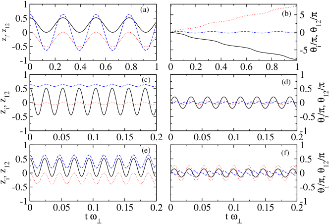
Figure 1: (Color online) Macroscopic quantum tunneling in the presence of a SO term. (a) population imbalances $z_{1}$ (solid black line), $z_{2}$ (dotted red line), and polarization $z_{12}$ (dashed blue line) when $\Lambda_{S}=10$ in the absence of tunneling ($J=0$)). (b) corresponding phases. (c) and (d) population imbalances, polarization, and phases when $\Lambda_{S}=10$ in the presence of tunneling ($\Lambda_{J}=1$). (e) and (f) same when $\Lambda_{S}=2$. In all cases, $U=U_{12}=\tilde{\delta}=\Gamma=0$.Initial conditions: $z_{1}(0)=0.518$, $z_{2}(0)=0.002$, $z_{12}=0$, $\theta_{k}(0)=0$ ($k=1,2$), $\theta_{12}(0)=0$.

For the numerical results discussed in this section, we consider $N=10^{5}$, ⁸⁷Rb atoms, and that the wavelength of the two counter-propagating lasers is $\lambda\approx 10^{3}$ nm. Following Ref. so-bose1 , we introduce natural units for the momentum and energy as $k_{L}=\sqrt{2}\pi/\lambda$ and $E_{L}=\hbar^{2}k_{L}^{2}/(2m)$. The SO coupling is given by $v=E_{L}/\hbar k_{L}$ and therefore for $\omega_{\perp}=400\pi$Hz one obtains $\gamma=3.37$. Notice that $S_{\pm}$ is defined as an overlap integral (see Eq. (IV)). To keep the model simple we approximate the four on-site modes by Gaussian wave functions. In this case, the overlap integral is proportional to $\exp(-d^{2})$, $d$ being the distance between the minimum of each well and the origin. Then, both $S_{\pm}$ and $J$ can be tuned by varying the distance between the wells.

The SO coupling $v$ is independent on the detuning $\delta$ and the Rabi coupling $\Omega_{R}$. We assume that $\Omega_{R}$ can be tuned in the interval $\left[0,7E_{L}/\hbar\right]$, and then $\Gamma_{\mathrm{max}}=19.92$. $\bar{\delta}$ is proportional to $\exp(-d^{2})$ and can thus also be tuned by varying $d$. In the following, we take the scattering lengths $a_{1}\simeq a_{2}\simeq 101.8a_{0}$ mariona , with $a_{0}$ the Bohr atom radius which gives $U_{\mbox{ref}}\approx 0.0012$, where $U_{\mbox{ref}}=\displaystyle{\frac{2a_{00}}{a_{\perp}}\int dx(\phi^{\alpha}(x))^{4}}$, $a_{00}=101.8a_{0}$, and the integral performed on the whole real axis. We take this value of the interactions to refer all variables in the rest of the paper. We define $\Lambda_{J}\equiv U_{\mbox{ref}}N/J$, which is the usual variable quantifying the ratio between atom-atom interaction and tunneling in a single component bosonic Josephson junction. Similarly, we define the quantities $\Lambda_{S}\equiv U_{\mbox{ref}}N/S_{+}$, and $\Lambda_{D}\equiv U_{\mbox{ref}}N/\tilde{\delta}$. Finally, we assume that the interactions can be tuned with respect to the reference, and therefore we define $C_{U}\equiv U/U_{\mbox{ref}}$ and $C_{U_{12}}\equiv U_{12}/U_{\mbox{ref}}$.

Note that in this part of the paper, we shall take $U_{12}$=0 to make the effect of the spin-orbit coupling as clear and neat as possible. Let us note, however, that the effect of the repulsion between species has been discussed thoroughly in Refs. lobo ; xu ; satja ; diaz1 ; ajj1 ; ajj2 ; qiu ; rabijosephson ; brunonjp , where it was found that the conventional Josephson dynamics is crucially modified by this term, even leading to measure synchronization in some limits qiu13 . Particularly, the inter-species interaction induces the presence of new fixed points on the problem which are related to the repulsion between components. Nevertheless, we take into account the effect of the boson-boson repulsion in subsection V.4.

V.1 Some considerations about fixed points

Inspection of Hamiltonian (21) (or its many-body counterpart, Eqs. (41), (42), (44)) permits one to identify three different processes which interchange atoms between wells or components. The first one is the usual tunneling between both wells, and is given by the term $J\sqrt{N_{k}^{\alpha}N_{k}^{\alpha^{\prime}}}\cos\left(\theta_{k}^{\alpha}-\theta_{k}^{\alpha^{\prime}}\right)$ in Eq. (21). The second one is associated to the SO terms proportional to $S_{\pm}$ in Eq. (21), and couples the atoms of one species located in one well to the atoms of the second species located in the other well. The third one is given by the terms corresponding to the detuning $\tilde{\delta}$ in Eq. (21). This is a coupling between atoms of different species in the same well. Finally, we note that the Rabi frequency $\Gamma$ introduces an energy gap between both species in Eq. (21). In this work, we study the effect of the SO coupling, detuning, and Rabi frequencies in the well-known Josephson dynamics in double wells. We focus in the case in which the most populated species has certain population imbalance, and study the effect of the dynamics of this species on the second initially balanced species. To understand this problem, let us discuss briefly the fixed points of Eqs. (29)-(32) when SO coupling and detuning frequencies are considered.

In the absence of interactions and when all terms other than the tunneling energy vanish, the fixed points are the usual ones at $(z_{k}^{0},\theta_{k}^{0})=(0,n\pi)$, $n\in\mathbb{Z}$. In such a case, there is no process that can produce interchange of atoms between the two components. Therefore $z_{12}$ remains constant at its initial value. This picture changes when the other two processes are considered. In the presence of the SO coupling and tunneling, when all other terms vanish, one can prove that Eqs. (29)-(32) vanish for $(z_{k}^{0},\theta_{k}^{0})=(z_{12}^{0},\theta_{12}^{0})=(0,0)$. When initially $z_{12}$ is different from zero and all other variables vanish, the population imbalances $z_{k}$ and the phase $\theta_{12}$ will remain in their initial value, while the equations of motion can be reduced to

$$\dot{z}_{12}=-2S_{+}\sin\bar{\theta}\sqrt{1-z_{12}^{2}},$$ (33)

$$\dot{\bar{\theta}}=2S_{+}\cos\bar{\theta}\frac{z_{12}}{\sqrt{1-z_{12}^{2}}},$$ (34)

with $\bar{\theta}=(\theta_{1}+\theta_{2})/2$. Therefore, both $z_{12}$ and $\bar{\theta}$ will oscillate during the evolution. In such a case, we observe numerically that $\theta_{1}$ and $\theta_{2}$ grow unbounded, with opposed sign. In addition, when initially all variables are zero except for $z_{k}$, the polarization $z_{12}$ remains at its initial value at zero. On the other hand, $(\theta_{1}+\theta_{2})/2$ and $z_{1}+z_{2}$ will oscillate, with the latter bounded by $\pm(z_{1}(0)+z_{2}(0))$, while $\theta_{12}$ also oscillates. We observe numerically that $z_{1}-z_{2}=z_{1}(0)-z_{2}(0)$ along evolution.

In the presence only of detuning, Eqs. (29)-(32) vanish for $(z_{k}^{0},\theta_{k}^{0})=(0,0)$, but now it is necessary that $(z_{12}^{0},\theta_{12}^{0})=(0,\pi)$. When initially $z_{12}$ is different from zero, $\theta_{12}=\pi$, and all other variables vanish, the population imbalances $z_{k}$ and the phase $\theta_{12}$ will remain in their initial value, while the equations of motion can be reduced to

$$\dot{z}_{12}=-2\tilde{\delta}\cos\tilde{\theta}\sqrt{1-z_{12}^{2}},$$ (35)

$$\dot{\tilde{\theta}}=-4\tilde{\delta}\sin\tilde{\theta}\frac{z_{12}}{\sqrt{1-z_{12}^{2}}},$$ (36)

with $\tilde{\theta}=(\theta_{1}-\theta_{2})/2$. Therefore, both $z_{12}$ and $\tilde{\theta}$ will oscillate during the evolution. In case $z_{k}$ are different from zero initially, while $z_{12}$ is zero, both $(\theta_{1}-\theta_{2})/2$ and $z_{1}-z_{2}$ will oscillate, with the latter bounded by $\pm(z_{1}(0)-z_{2}(0))$. Now, $z_{12}$ remains at its initial value, $\theta_{12}$ also oscillates, and we observe numerically that $z_{1}+z_{2}=z_{1}(0)+z_{2}(0)$.

In the next section we study how the fixed point analysis briefly discussed above can help to understand the dynamics when the most populated species has certain population imbalance, while the second species is balanced, that is initially $z_{12}$ and $z_{1}$ are non-zero, while $z_{2}$ is zero. To illustrate this situation we consider in all numerical examples to be discussed in the next subsections that initially $z_{1}=0.518$, $z_{2}=0.002$, $z_{12}=0.64$ and all initial phases are zero unless explicitly indicated.

V.2 Macroscopic quantum tunneling and self-trapping in the presence of Spin-Orbit coupling

We first assume $\bar{\delta}=\Gamma=0$, and study the effect of the SO coupling $v$. This coupling is associated to the kinetic moment $p_{x}$ or $p_{y}$ of the atoms in each species (see Eq. (1)). As we have shown, when the single particle 3D potential can be reduced effectively to a 1D double-well, where the dynamics in transverse directions is essentially frozen, the SO coupling, proportional to $S_{\pm}$, becomes apparent in a non-trivial way in the equations of motion.

The SO coupling term allows for the complete transfer of the atoms of species 1 in the left well to species 2 in the right well (see Fig.1a-b), when no other term is considered. In the presence of a tunneling term which dominates the SO coupling, see Figs. 1c-d, $z_{1}$ shows fast Rabi oscillations, where its corresponding phase is bounded. This can be understood in view of Eqs. (29) and (31), as in the presence of a tunneling which dominates over $S_{\pm}$, these equations will only vanish if $\theta_{k}=0,\pi,\dots$ Therefore, in this case $\theta_{k}$ cannot grow unbounded and has to oscillate around $\theta_{k}=0$. A small transfer of atoms between both components still occurs, but it is not enough to transfer all population from component 1 to component 2 before it tunnels to the other well. If $S_{\pm}$ are comparable to $J$, both effects are combined, and the transfer of atoms between components is enlarged and the tunneling of the atoms of component 1 is reduced, as shown in Figs. 1e-f.

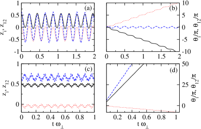
Figure 2: (Color online) Macroscopic quantum self-trapping in the presence of a SO term. (a) population imbalances $z_{1}$, $z_{2}$, and polarization $z_{12}$ when $\Lambda_{S}=10$ when the interactions are small, $C_{U}=1/5$. Same color conventions as in Fig. 1. (b) corresponding phases. (c) and (d) self-trapping induced by the interactions ($\Lambda_{S}=10,\,C_{U}=5$). In all cases, $U_{12}=J=\tilde{\delta}=\Gamma=0$. Initial conditions as in Fig. 1.

Let us now illustrate the effect of the interactions on the dynamics induced by the SO coupling shown in Figs. 1a-b corresponding to the absence of hopping and interactions. In the presence of a small interaction term, the transfer of atoms between components associated with the dynamical evolution of the polarization $z_{12}$ still occurs. The interactions only modulate slightly this dynamics, as shown in Figs. 2a-b. Conversely, for larger $U$, self-trapping occurs in all variables, and correspondingly all phases are running (see Figs. 2c-d). When both tunneling and interactions are different from zero, self-trapping can occur independently on the polarization, $z_{12}$, and the population imbalances, $z_{k}$. In Figs. 3a-b we show the dynamics when the interactions dominate over the SO term, but not over the tunneling, which induces self-trapping on $z_{12}$, while $z_{k}$ still oscillates. Increasing further the interactions produces self-trapping also in $z_{k}$, as plotted in Figs. 3c-d. We conclude this subsection with a remark about Figs. 1a-b. The phase $(\theta_{1}+\theta_{2})/2$ oscillates accordingly with $\theta_{1}$ and $\theta_{2}$ growing unbounded with opposed sign (see Eq. (33)). Moreover, because $z_{k}$ are different from zero initially, $z_{1}+z_{2}$ oscillates, while $z_{1}-z_{2}=z_{1}(0)-z_{2}(0)=0.516$ along all the evolution, and $\theta_{12}$ oscillates, in accordance with the discussion on section V.1.

V.3 Macroscopic quantum tunneling and self-trapping in the presence of the Rabi and detuning frequencies

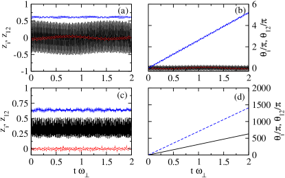
Figure 3: (Color online) Macroscopic quantum tunneling and self-trapping in the presence of a SO term. (a) population imbalances $z_{1}$, $z_{2}$, and polarization $z_{12}$ for $\Lambda_{S}=10$ when the interactions are small ($C_{U}=1/10$) in the presence of tunneling, $\Lambda_{J}=1$, showing self-trapping dynamics of $z_{12}$. Same color conventions as in Fig. 1. (b) corresponding phases. (c) and (d) self-trapping dynamics in all variables when $\Lambda_{S}=10$ and $C_{U}=25$. In all cases, $U_{12}=\tilde{\delta}=\Gamma=0$. Initial conditions as in Fig. 1.

Let us now discuss on the effect of the Rabi and detuning frequencies, $\Gamma$ and $\bar{\delta}$, respectively. The detuning frequency induces a local transfer of population between both components. To illustrate this, we represent in Figs. 4a-b the dynamics when all other terms are zero and the tunneling $J$ is very small, when initially $\theta_{12}=\pi$, and all other phases vanish. According to Eq. (35), the corresponding dynamics will be oscillatory around the fixed point, with $\theta_{1}-\theta_{2}$ also oscillating. Because initially $z_{1}=0.518$ and $z_{2}=0.002$, $z_{1}-z_{2}$ also oscillates with $z_{1}+z_{2}=z_{1}(0)+z_{2}(0)=0.52$ along all the evolution. Again, $\theta_{12}$ also oscillates, in accordance with the discussion in section V.1. For larger $J$, the atoms of each species tunnel also to the other well in the same time scales, as shown in Figs. 4c-d. Differently from the dynamics in the presence of the SO term, $\theta_{1}$ and $\theta_{2}$ do not grow unbounded in the absence of tunneling. Therefore, atoms can still be transformed from component 1 to component 2 in the presence of large tunneling. This effect is quicker if $J$ is increased further, as illustrated in Figs. 4e-f. The dynamics of $z_{12}$ is not affected by the Josephson physics. This is due to the fact that the detuning term induces local population transfer, similarly to the transfer of populations among the different Zeeman components in a spinor BEC spinor . In Fig. 5 we reproduce the same cases when initially $\theta_{12}=0$. As this initial condition does not correspond to a fixed point, the phase oscillates abruptly and $z_{12}$ oscillates in the interval $[-1,1]$, as it possibly corresponds to an initial condition close to a separatrix. In Figs. 6a-b we show that the interactions can induce self-trapping in $z_{12}$ when the interactions dominate over the detuning term. If increased further, Figs. 6c-d, the interactions induce self-trapping in all variables.

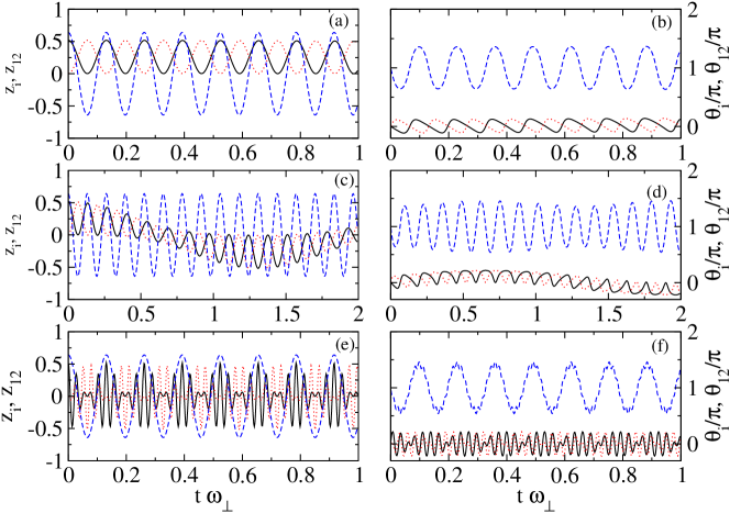
Figure 4: (Color online) Macroscopic quantum tunneling in the presence of a detuning $\tilde{\delta}$, when the initial phase for the polarization is $\theta_{12}(0)=\pi$. (a) population imbalances $z_{1}$, $z_{2}$, and polarization $z_{12}$ for $\Lambda_{D}=5$ when the tunneling term is very small $\Lambda_{J}=10^{3}$. Same color conventions as in Fig. 1. (b) corresponding phases. (c) and (d) same when $\Lambda_{J}=10^{2}$, and (e) and (f) when $\Lambda_{J}=1$. In all cases, $U=U_{12}=S_{\pm}=\Gamma=0$. Initial conditions for $z_{k}$, $\theta_{k}$ ($k=1,2$), and $z_{12}$ as in Fig. 1.

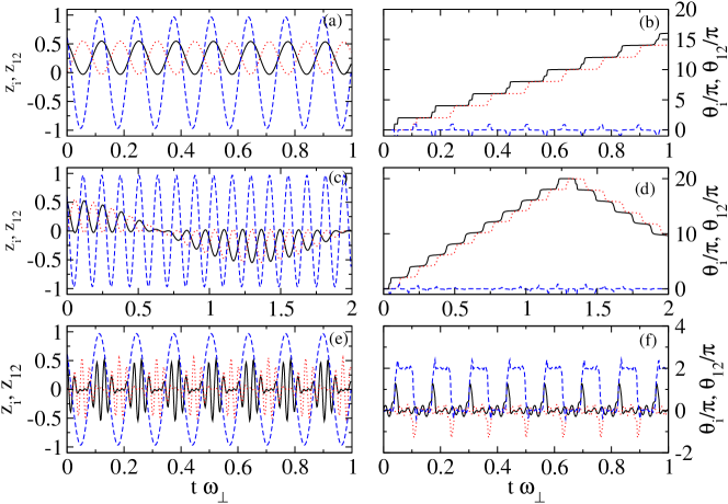
Figure 5: (Color online) Macroscopic quantum tunneling in the presence of a detuning $\tilde{\delta}$, when the initial phase for the polarization is $\theta_{12}(0)=0$. (a) population imbalances $z_{1}$, $z_{2}$, and polarization $z_{12}$ for $\Lambda_{D}=5$ when the tunneling term is very small $\Lambda_{J}=10^{3}$. Same color conventions as in Fig. 1. (b) corresponding phases. (c) and (d) same when $\Lambda_{J}=10^{2}$, and (e) and (f) when $\Lambda_{J}=1$. In all cases, $U=U_{12}=S_{\pm}=\Gamma=0$. Initial conditions $z_{k}$, $\theta_{k}$ ($k=1,2$), and $z_{12}$ as in Fig. 1.

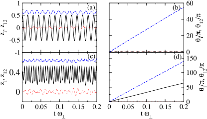
Figure 6: Macroscopic quantum self-trapping in the presence of a detuning $\tilde{\delta}$, when initially $\theta_{12}(0)=0$. (a) population imbalances $z_{1}$, $z_{2}$, and polarization $z_{12}$ when $\Lambda_{D}=5$, $\Lambda_{J}=1$, $C_{U}=10$, and all other terms vanish, showing self-trapping dynamics of $z_{12}$. Same color conventions as in Fig. 1. (b) corresponding phases. (c) and (d) self-trapping in all variables when the interactions are increased to $C_{U}=25$. Initial conditions for $z_{k}$, $\theta_{k}$ ($k=1,2$), and $z_{12}$ as in Fig. 1.

The effect of the Rabi frequency on the dynamics associated with $S_{\pm}$ and $\delta$ can be understood in view of the equations of motion for $\theta_{12}$, Eq. (32), as $\Gamma$ appears as a constant in the equation. Therefore, it introduces an energy gap between both components, which, when it dominates over the rest of terms, forces $\theta_{12}$ to be a running phase, similarly to the problem of bosons in an excited level in double wells 2014Gilletarxiv . In Figs. 7a-b we show the effect of $\Gamma$ in the oscillations of the polarization $z_{12}$ due to the effect of the SO coupling $S_{\pm}$. We observe that the oscillation of the polarization is reduced with respect to the case of Figs. 1a-b, and $\theta_{12}$ is a running phase. Then, the effect of $\Gamma$ is to inhibit the coupling of the two components associated to the SO term. Similarly, in Figs. 7c-d we observe that $\Gamma$ again reduces (with respect to the case of Figs. 5e-f) the oscillations on $z_{12}$ induced by the detuning frequency $\delta$, again decoupling the dynamics of the two components.

V.4 Effect of the inter-species interaction

As commented before, in the previous results we have decided to set the inter-species interaction $U_{12}$ to zero, to emphasize the effects of the spin-orbit coupling, Rabi and detuning frequencies. In a possible experimental realization along the lines of the recent SO experiments so-bose1 it may be difficult to experimentally achieve this limiting case. For the case of considering two of the Zeeman states of the $F=1$ ⁸⁷Rb one has that $U_{1}\approx U_{2}\approx U_{12}$ brunonjp . The inter-species interactions has profound and diverse effects on the Josephson dynamics of two components in double wells lobo ; xu ; satja ; diaz1 ; ajj1 ; ajj2 ; qiu ; rabijosephson ; brunonjp ; 2014Gilletarxiv , and therefore an extensive discussion on this topic is out of the scope of this paper. If the inter-species interaction $U_{12}$ is similar to intra-species ones ($U_{1}$ and $U_{2}$), and for the case considered here of a polarized initial state, the dynamics of the less populated species is crucially influenced by the dynamics of the most populated one diaz1 . Moreover, for a value of $U_{12}$ above certain threshold, both species cover the same region in the phase portrait, an effect known as measurement synchronization (MS) qiu ; qiu13 . In Figs. 8a-b we show the dynamics of the system when all the detunings and the SO coupling term vanish. Here, the value of $U_{12}$ is below the MS threshold, as can be seen from the fact that $z_{1}$ and $z_{2}$ have different maximum amplitudes. In Figs. 8c-d we have increased slightly the SO term, and some transfer of atoms between both species occurs. If the interactions dominate over the tunneling and the SO term (for example, as in Figs. 2c-d), all variables are self-trapped and the corresponding phases grow. In Figs. 6g-h Figs. 8e-f we plot the same case as in Figs. 2c-d for non-zero inter- species interactions. Moreover, the evolution of $z_{2}$ is slightly dragged by that of $z_{1}$, an effect which is in accordance with the results of Ref. diaz1 . We have also observed numerically that the phenomena associated with the detuning and Rabi frequencies described above still occur in the presence of the inter-species energy.

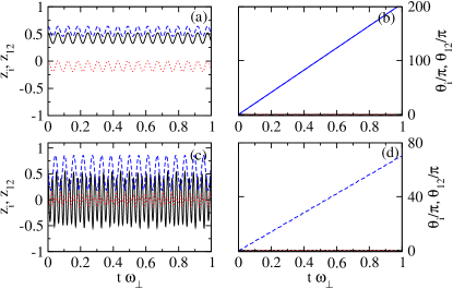
Figure 7: Decoupling induced by the Rabi frequency, $\Gamma$. (a) population imbalances $z_{1}$, $z_{2}$, and polarization $z_{12}$ when $\Lambda_{S}=10$, $\Gamma=50$, and all other terms vanish. Same color conventions as in Fig. 1. (b) corresponding phases. (c) and (d) same when $\Lambda_{D}=5$, $\Gamma=50$, $\Lambda_{J}=1$, and all other terms vanish. Initial conditions as in Fig. 1.

As a conclusive remark, we note that working within the single-particle Hamiltonian framework corresponding to Eq. (1) produces changes with respect to the results achieved by Zhang et al. zhang . In fact in our case, the spin-orbit coupling induces change in polarization (the external josephson is transferred into internal) while in the case of zhang it affects the tunneling rate.

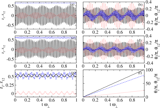
Figure 8: Macroscopic quantum tunneling and self-trapping in the presence of SO coupling and inter-species interactions $U_{12}$. (a) population imbalances $z_{1}$, $z_{2}$, and polarization $z_{12}$ when $C_{U}=C_{U_{12}}=1/2$ and $\Lambda_{J}=1$, and all other terms vanish, reproducing two-component dynamics in the absence of SO coupling. Same color conventions as in Fig. 1. (b) corresponding phases. (c) and (d) effect of the SO coupling term when $\Lambda_{S}=10$. (e), (f) dragging of $z_{2}$ by $z_{1}$ in the self-trapping dynamics, when $\Lambda_{S}=10$, $C_{U}=5$, $C_{U_{12}}=1$, and all other terms vanish. Initial conditions as in Fig. 1.

VI Summary and conclusions

The recent developments in ultracold atomic gases, namely the experimental realization of external bosonic Josephson junctions, together with the artificial creation of spin-orbit coupling for ultracold atoms paved the way to discuss the interplay between both effects in a common set-up. As we have described, the conventional macroscopic quantum tunneling or self-trapping scenarios of two bosonic components confined in a double-well determine crucially the polarization induced by the spin-orbit (SO) coupling. We have shown that the SO coupling transfers atoms between both components in different wells. This population transfer induced by the SO term depends on how this energy compares with the tunneling and interaction energy. In the macroscopic quantum tunneling limit this transfer is large if it dominates over the tunneling energy. By increasing the interactions we observe that one can induce the self-trapping of the polarization variable and subsequently of the population imbalance. Secondly, we have studied the effect of the Rabi and detuning frequencies. We have shown that the effect of the Rabi frequency is to decouple both components, and thus reduce the population transfer between the two species. On the contrary, the effect of the detuning frequency is a coupling between both components in the same well. Now, this transfer occurs even in the presence of large tunneling energy, though in different time scales. The interactions produce also self-trapping in all variables if they dominate over the tunneling and detuning. Finally, we have shown that the phenomena associated with the SO coupling, detuning and Rabi frequencies are robust in the presence of inter-species interactions.

Appendix A Many-Body Hamiltonian for the spin-orbit effect in double-wells

The second quantized Hamiltonian for $N$ interacting two-component bosons of equal mass $m$ confined by an external potential $U(\mathbf{r})$ in terms of the creation-annihilation field operators - $\hat{\Psi}(\mathbf{r})$, $\hat{\Psi}^{\dagger}(\mathbf{r})$ - in the presence of spin-orbit coupling is

$$\hat{H} =\int d\mathbf{r}\hat{\Psi}^{\dagger}(\mathbf{r})H_{\mathrm{sp}}\hat{\Psi}(\mathbf{r})$$ (37)

$$+\frac{1}{2}\int d\mathbf{r}\hat{\Psi}^{\dagger}(\mathbf{r})\left[\int d\mathbf{x^{\prime}}\hat{\Psi}^{\dagger}(\mathbf{r}^{\prime})V_{int}(\mathbf{r}-\mathbf{r}^{\prime})\hat{\Psi}(\mathbf{r})\right]\hat{\Psi}(\mathbf{r}),$$

where $V_{int}(\mathbf{r}-\mathbf{r}^{\prime})$ stands for the two-body interaction, and $\hat{\Psi}$ and $\hat{\Psi}^{\dagger}$ are two-component vectors. Here $H_{\mathrm{sp}}$ is

$$H_{\mathrm{sp}} = \left(-\frac{\hbar^{2}}{2m}\nabla^{2}+U(\mathbf{r})\right)\sigma_{0}+v_{R}\left(p_{x}\sigma_{y}-p_{y}\sigma_{x}\right)$$ (38)

$$+ v_{D}\left(p_{x}\sigma_{y}+p_{y}\sigma_{x}\right)+\frac{\Omega_{R}}{2}\sigma_{z}+\frac{\delta}{2}\sigma_{y},$$

with $\sigma_{0}$ the $2\times 2$ identity matrix, and $\sigma_{x,y,z}$ the Pauli matrices. Let us write $\hat{\Psi}(\mathbf{r})=\left(\hat{\Psi}_{1}(\mathbf{r}),\hat{\Psi}_{2}(\mathbf{r})\right)$, where the index $1$ ($2$) accounts for the first (second) component. We consider contact interactions both for intra-species interaction and for inter-species one. This means that the interatomic potential for the former case is assumed to be $g_{k}\delta(\mathbf{r}-\mathbf{r}^{\prime})$ ($g_{k}=4\pi\hbar^{2}a_{k}/m$ with $a_{k}$ the intra-species $s$-wave scattering length), while for the latter $g_{12}\delta(\mathbf{r}-\mathbf{r}^{\prime})$ ($g_{12}=4\pi\hbar^{2}a_{12}/m$ with $a_{12}$ the inter-species $s$-wave scattering length). Then, the interacting part of the Hamiltonian can be written in the following way

$$\hat{H}_{\mathrm{int}} \!=\! \sum_{k=1,2}\frac{g_{k}}{2}\!\int d\mathbf{r}\hat{\Psi}_{k}^{\dagger}\hat{\Psi}_{k}^{\dagger}\hat{\Psi}_{k}\hat{\Psi}_{k}+g_{12}\!\int d\mathbf{r}\hat{\Psi}_{1}^{\dagger}\hat{\Psi}_{2}^{\dagger}\hat{\Psi}_{2}\hat{\Psi}_{1}.$$

We can write the Hamiltonian as $\hat{H}=\hat{H}_{1}+\hat{H}_{2}+\hat{H}_{12}$ with

$$\hat{H}_{1} \!=\! \int d\mathbf{r}\hat{\Psi}_{1}^{\dagger}H_{\mathrm{sp}}^{1}\hat{\Psi}_{1}+\frac{g_{1}}{2}\int d\mathbf{r}\hat{\Psi}_{1}^{\dagger}\hat{\Psi}_{1}^{\dagger}\hat{\Psi}_{1}\hat{\Psi}_{1}$$ (39)

and similarly for species 2. Here, the single particle Hamiltonian is $H_{\mathrm{sp}}^{k}=\displaystyle{\left(-\frac{\hbar^{2}}{2m}\nabla^{2}+U(\mathbf{r})\pm\Omega_{R}/2\right)}$ with the plus or minus for $1$ and $2$, respectively. The part of the Hamiltonian which couples both bosonic species is

$$\hat{H}_{12} \!=\!\hbar\int\!d\mathbf{r}\hat{\Psi}_{1}^{\dagger}\left[v_{R}\left(-\partial_{x}+i\partial_{y}\right)+v_{D}\left(-\partial_{x}-i\partial_{y}\right)\right]\hat{\Psi}_{2}$$

$$\!+\!\hbar\int\!d\mathbf{r}\hat{\Psi}_{2}^{\dagger}\left[v_{R}\left(\partial_{x}+i\partial_{y}\right)+v_{D}\left(\partial_{x}-i\partial_{y}\right)\right]\hat{\Psi}_{1}$$ (40)

$$\!+\!g_{12}\int\!d\mathbf{r}\hat{\Psi}_{1}^{\dagger}\hat{\Psi}_{2}^{\dagger}\hat{\Psi}_{2}\hat{\Psi}_{1}\!-\!i\!\int\!d\mathbf{r}\hat{\Psi}_{1}^{\dagger}\frac{\delta}{2}\hat{\Psi}_{2}+\!i\!\int\!d\mathbf{r}\hat{\Psi}_{2}^{\dagger}\frac{\delta}{2}\hat{\Psi}_{1}\;.$$

We assume a separable potential, with harmonic confinement in the $y$ and $z$ directions and a double-well in the $x$ direction $U(\mathbf{r})=\frac{1}{2}m\omega_{\perp}^{2}(y^{2}+z^{2})+V_{DW}(x)$. Let us write $\hat{\Psi}_{1}(\mathbf{r})=\hat{a}_{L}\psi_{1}^{L}(\mathbf{r})+\hat{a}_{R}\psi_{1}^{R}(\mathbf{r})$ and $\hat{\Psi}_{2}(\mathbf{r})=\hat{b}_{L}\psi_{2}^{L}(\mathbf{r})+\hat{b}_{R}\psi_{2}^{R}(\mathbf{r})$, with $\hat{a}_{L(R)}$ and $\hat{b}_{L(R)}$ operators annihilating a boson of the species 1 and a boson of the species 2, respectively, in the left (right) well. These single-particle operators obey the usual boson-commutation relations. For the orbitals $\psi_{k}^{\alpha}(\mathbf{r})$ we use Gaussian-like functions for the $y$ and $z$ directions (i.e., the ground-state wave function of the harmonic oscillator $m\omega_{\perp}^{2}y^{2}/2$ times that of the harmonic oscillator $m\omega_{\perp}^{2}z^{2}/2$) and on-well localized functions $w_{k}^{\alpha}(x)$ ($\int dxw_{k}^{\alpha*}w_{k}^{\alpha^{\prime}}=\delta_{\alpha,\alpha^{\prime}}$) in the $x$ direction. In such a way, we have that $\psi_{k}^{\alpha}(\mathbf{r})=\frac{1}{\sqrt{\pi}a_{\perp}}\exp\left(-\frac{y^{2}+z^{2}}{2a_{\perp}^{2}}\right)w_{k}^{\alpha}(x)$ with $a_{\perp}=\sqrt{\hbar/m\omega_{\perp}}$, $k=1,2$ and $\alpha=L,R$. Then, we obtain

$$\hat{H}=\hat{H}_{1}+\hat{H}_{2}+\hat{H}_{12}.$$ (41)

The first two terms are

$$\hat{H}_{1}=(\hat{n}_{1}^{L}+\hat{n}_{1}^{R})\varepsilon_{1}-J_{1}\sum_{\alpha\neq\alpha^{\prime}}\hat{a}_{\alpha}^{\dagger}\hat{a}_{\alpha^{\prime}}+\frac{U_{1}}{2}\sum_{\alpha}\hat{n}_{1}^{\alpha}\left(\hat{n}_{1}^{\alpha}-1\right),$$ (42)

where $\hat{n}_{1}^{\alpha}=\hat{a}_{\alpha}^{\dagger}\hat{a}_{\alpha}$, and similarly for $k=2$. Here and in the following $\sum_{\alpha}$ is a shorthand notation for $\sum_{\alpha=L,R}$. We have used the following constants

$$E_{k} = \int\!d\mathbf{r}\,\psi_{k}^{\alpha*}(\mathbf{r})\left(-\frac{\hbar^{2}}{2m}\nabla^{2}+U(\mathbf{r})\right)\psi_{k}^{\alpha}(\mathbf{r}),$$

$$\sigma = \frac{\Omega_{R}}{2}\int\!d\mathbf{r}\,\psi_{k}^{\alpha*}(\mathbf{r})\psi_{k}^{\alpha}(\mathbf{r}),$$

$$J_{k} = -\int\!d\mathbf{r}\,\psi_{k}^{\alpha*}(\mathbf{r})\left(-\frac{\hbar^{2}}{2m}\nabla^{2}+U(\mathbf{r})\right)\psi_{k}^{\alpha^{\prime}}(\mathbf{r}),$$

$$U_{k} = g_{k}\int\!d\mathbf{r}|\psi_{k}^{\alpha}(\mathbf{r})|^{4}\;,$$ (43)

and $\varepsilon_{k}=E_{k}\pm\sigma$, where the minus sign holds for $k=2$. The inter-species term is

$$\hat{H}_{12} = \sum_{\alpha}(S_{12}^{\alpha}+i\ D_{12}^{\alpha})\hat{a}_{\alpha}^{\dagger}\hat{b}_{\alpha}+\sum_{\alpha\neq\alpha^{\prime}}\bar{S}_{12}^{\alpha,\alpha^{\prime}}\hat{a}_{\alpha}^{\dagger}\hat{b}_{\alpha^{\prime}}$$ (44)

$$+ \sum_{\alpha}(S_{21}^{\alpha}+i\ D_{21}^{\alpha})\hat{b}_{\alpha}^{\dagger}\hat{a}_{\alpha}+\sum_{\alpha\neq\alpha^{\prime}}\bar{S}_{21}^{\alpha,\alpha^{\prime}}\hat{b}_{\alpha}^{\dagger}\hat{a}_{\alpha^{\prime}}$$

$$+ U_{12}\sum_{\alpha}\hat{n}_{1}^{\alpha}\hat{n}_{2}^{\alpha},$$

with

$$U_{12}\! = \!g_{12}\int d\mathbf{r}\psi_{1}^{\alpha*}(\mathbf{r})\psi_{2}^{\alpha*}(\mathbf{r})\psi_{2}^{\alpha}(\mathbf{r})\psi_{1}^{\alpha}(\mathbf{r}),$$ (45)

$$S_{12}^{\alpha}\! = \!\int\!\!d\mathbf{r}\psi_{1}^{\alpha*}\hbar\left[v_{R}\left(-\partial_{x}+i\partial_{y}\right)\!+\!v_{D}\left(-\partial_{x}-i\partial_{y}\right)\right]\psi_{2}^{\alpha},$$

$$S_{21}^{\alpha}\! = \!\int\!\!d\mathbf{r}\psi_{2}^{\alpha*}\hbar\left[v_{R}\left(\partial_{x}+i\partial_{y}\right)\!+\!v_{D}\left(\partial_{x}-i\partial_{y}\right)\right]\psi_{1}^{\alpha},$$

$$\bar{S}_{12}^{\alpha,\alpha^{\prime}}\! = \!\int\!\!d\mathbf{r}\psi_{k}^{\alpha*}\hbar\left[v_{R}\left(-\partial_{x}+i\partial_{y}\right)\!+\!v_{D}\left(-\partial_{x}-i\partial_{y}\right)\right]\psi_{k^{\prime}}^{\alpha^{\prime}},$$

$$\bar{S}_{21}^{\alpha,\alpha^{\prime}}\! = \!\int\!\!d\mathbf{r}\psi_{2}^{\alpha*}\hbar\left[v_{R}\left(\partial_{x}+i\partial_{y}\right)\!+\!v_{D}\left(\partial_{x}-i\partial_{y}\right)\right]\psi_{1}^{\alpha^{\prime}},$$

$$D_{12}^{\alpha}\! = \!-\int d\mathbf{r}\psi_{1}^{\alpha*}\frac{\delta}{2}\psi_{2}^{\alpha},\,\,\,\,D_{21}^{\alpha}=\int d\mathbf{r}\psi_{2}^{\alpha*}\frac{\delta}{2}\psi_{1}^{\alpha}.$$

Non-zero inter-well interacting terms have been neglected, as commonly assumed in standard two- or four-mode Hamiltonians 1999SpekkensPRA ; 2011GarciaMarchPRA ; 2012GarciaMarchFiP . This Hamiltonian conserves the number of atoms as it commutes with the total number operator $\hat{N}=\sum_{k,\alpha}\hat{n}_{k}^{\alpha}$. For $v_{R}=v_{D}=v$ the coefficients given in Eqs. (45) are the following

$$S_{12}^{\alpha}\! = \!-2\hbar v\int d\mathbf{r}\,\psi_{1}^{\alpha*}(\mathbf{r})\partial_{x}\psi_{2}^{\alpha}(\mathbf{r}),$$ (46)

$$S_{21}^{\alpha}\! = \!2\hbar v\int d\mathbf{r}\,\psi_{2}^{\alpha*}(\mathbf{r})\partial_{x}\psi_{1}^{\alpha}(\mathbf{r}),$$

$$\bar{S}_{12}^{\alpha,\alpha^{\prime}}\! = \!-2\hbar v\int d\mathbf{r}\,\psi_{1}^{\alpha*}(\mathbf{r})\partial_{x}\psi_{2}^{\alpha^{\prime}}(\mathbf{r})$$

$$\bar{S}_{21}^{\alpha,\alpha^{\prime}}\! = \!2\hbar v\int d\mathbf{r}\,\psi_{2}^{\alpha*}(\mathbf{r})\partial_{x}\psi_{1}^{\alpha^{\prime}}(\mathbf{r}),$$

$$D_{12}^{\alpha}\! = \!-\frac{\delta}{2}\!\int\!d\mathbf{r}\,\psi_{1}^{\alpha*}(\mathbf{r})\psi_{2}^{\alpha}(\mathbf{r}),\,D_{21}^{\alpha}\!=\!\frac{\delta}{2}\!\int\!d\mathbf{r}\,\psi_{2}^{\alpha*}(\mathbf{r})\psi_{1}^{\alpha}(\mathbf{r}).$$

By integrating by parts, we get that $S_{12}^{\alpha}=S_{21}^{\alpha}$ and $\bar{S}_{12}^{\alpha,\alpha^{\prime}}=\bar{S}_{21}^{\alpha^{\prime},\alpha}$. We also notice that $\bar{S}_{12}^{L,R}=-\bar{S}_{12}^{R,L}$ and that $D_{12}^{\alpha}=-D_{21}^{\alpha}$. Then, by calling $S=S_{12}^{\alpha}$, $S_{+}=\bar{S}_{12}^{L,R}=\bar{S}_{21}^{R,L}$, $S_{-}=\bar{S}_{12}^{R,L}=\bar{S}_{21}^{L,R}$, and $\tilde{\delta}=D_{12}^{\alpha}$, we can write Eq. (44) as

$$\hat{H}_{12} = \sum_{\alpha}(S+i\tilde{\delta})\hat{a}_{\alpha}^{\dagger}\hat{b}_{\alpha}+\mbox{h.c.}+U_{12}\sum_{\alpha}\hat{n}_{1}^{\alpha}\hat{n}_{2}^{\alpha}$$ (47)

$$+ S_{+}\hat{a}_{L}^{\dagger}\hat{b}_{R}+\mbox{h.c.}+S_{-}\hat{b}_{L}^{\dagger}\hat{a}_{R}+\mbox{h.c.}$$

We have checked that this Hamiltonian conserves the number of atoms. Notice that there are four different processes that interchange atoms between both species. The first two, associated to $S$ and $\tilde{\delta}$, interchange atoms between $k$ and $l$ components located in the same well. The third term, associated to $S_{+}$ interchanges atoms of $k$ component located in the left well and atoms of $l$ component located in the right well. The last term, $S_{-}$, transforms atoms of $k$ in the right well to atoms of $l$ in the left well, and vice-versa. From the Heisenberg equations of motion for the operators $\hat{a}_{\alpha}$ and $\hat{b}_{\alpha}$

$$i\hbar\frac{d\hat{a}_{\alpha}}{dt}=\left[\hat{a}_{\alpha},\hat{H}\right]\,\,\,\mbox{and}\,\,i\hbar\frac{d\hat{b}_{\alpha}}{dt}=\left[\hat{b}_{\alpha},\hat{H}\right]$$ (48)

one can obtain

$$i\hbar\frac{d\hat{a}_{\alpha}}{dt} = -J_{1}\hat{a}_{\alpha^{\prime}}+U_{1}\hat{n}_{1}^{\alpha}\hat{a}_{\alpha}+\varepsilon_{1}\hat{a}_{\alpha}+U_{12}\hat{n}_{2}^{\alpha}\hat{a}_{\alpha}$$ (49)

$$- S\hat{b}_{\alpha}-\bar{S}_{\pm}\hat{b}_{\alpha^{\prime}}-i\tilde{\delta}\hat{b}_{\alpha},$$

$$i\hbar\frac{d\hat{b}_{\alpha}}{dt} = -J_{2}\hat{b}_{\alpha^{\prime}}+U_{2}\hat{n}_{2}^{\alpha}\hat{b}_{\alpha}+\varepsilon_{2}\hat{b}_{\alpha}+U_{12}\hat{n}_{1}^{\alpha}\hat{b}_{\alpha}$$ (50)

$$- S\hat{a}_{\alpha}-\bar{S}_{\mp}\hat{a}_{\alpha^{\prime}}+i\tilde{\delta}\hat{a}_{\alpha},$$

and their corresponding Hermitian conjugates. The upper(lower) sign in the $S_{\pm}$ coefficients apply to $\alpha=L(R)$. To reconcile the definition of the coefficients with the one given in Eqs. (IV) we have redefined all coefficients as positive, and therefore we have written the minus sign inside their definitions explicitly in the equations. We assume that the creation/annihilation operators behave as $c$-numbers, that is $a_{\alpha}=\sqrt{N_{1}^{\alpha}}e^{i\phi_{1}^{\alpha}}$ where $N_{1}^{\alpha}=|a_{\alpha}|^{2}$ is the number of particles of species 1 and $\phi_{1}^{\alpha}$ is a phase (similarly $b_{\alpha}=\sqrt{N_{2}^{\alpha}}e^{i\phi_{2}^{\alpha}}$). After some algebra, the equations of motion for the number of particles, Eq. (19), and phases, Eq. (20), are obtained from the equations of motion (49)-(50). Since we assumed that $m_{1}=m_{2}=m$, and therefore one can use the same localized function for the two components, we obtain that $S=0$ and $\epsilon_{1}=\epsilon_{2}$, and consequently the corresponding terms are absent in Eqs. (19)-(20).

References

• (1) Y.J. Lin, K. Jimenez-Garcia, and I.B. Spielman, Nature 471, 83 (2011).
• (2) P. Wang, Z. Yu, Z. Fu, J. Miao, L. Huang, S. Chai, H. Zhai, and J. Zhang, Phys. Rev. Lett. 109, 095301 (2012).
• (3) L.W. Cheuk, A. T. Sommer, Z. Hadzibabic, T. Yefsah, W. S. Bakr, and M. W. Zwierlein, Phys. Rev. Lett. 109, 095302 (2012).
• (4) Y. A. Bychov and E. I. Rashba, J. Phys. C 17, 6029 (1984).
• (5) G. Dresselhaus, Phys. Rev. 100, 580 (1955).
• (6) G. I. Martone, Y. Li, L. P. Pitaevskii, and S. Stringari, Phys. Rev. A 86, 063621 (2012).
• (7) Y. Li, G. I. Martone, L. P. Pitaevskii, and S. Stringari, Phys. Rev. Lett. 110, 235302 (2013).
• (8) W. S. Cole, S. Zhang, A. Paramekanti, and N. Trivedi, Phys. Rev. Lett 109, 085302 (2012).
• (9) L. Salasnich and B. A. Malomed, Phys. Rev. A 87, 063625 (2013).
• (10) V. Achilleos, D.J. Frantzeskakis, P.G. Kevrekidis, and D.E. Pelinovsky, Phys. Rev. Lett. 110, 264101 (2013).
• (11) M. Burrello and A. Trombettoni, Phys. Rev. Lett. 105, 125304 (2010).
• (12) T. Grass, B. Juliá-Díaz, M. Burrello, M. Lewenstein, J. Phys. B: At. Mol. Opt. Phys. 46, 134006 (2013).
• (13) J. P. Vyasanakere, S. Zhang, and V. B. Shenoy, Phys. Rev. B 84, 014512 (2011); M. Gong, S. Tewari, and C. Zhang, Phys. Rev. Lett. 107, 195303 (2011); H. Hu, L. Jiang, X-J. Liu, and H. Pu, Phys. Rev. Lett. 107, 195304 (2011); Z-Q. Yu and H. Zhai, Phys. Rev. Lett. 107, 195305 (2011); M. Iskin and A. L. Subasi, Phys. Rev. Lett. 107, 050402 (2011); W. Yi and G.-C. Guo, Phys. Rev. A 84, 031608 (2011); M. Iskin and A. L. Subasi, Phys. Rev. A 84, 043621 (2011); L. Jiang, X.-J. Liu, H. Hu, and H. Pu, Phys. Rev. A 84, 063618 (2011); Li Han and C.A.R. Sa de Melo, Phys. Rev. A 85, 011606(R) (2012).
• (14) L. Dell’Anna, G. Mazzarella, and L. Salasnich, Phys. Rev. A 84, 033633 (2011); L. Dell’Anna, G. Mazzarella, and L. Salasnich, Phys. Rev. A 86, 053632 (2012).
• (15) K. Zhou, Z. Zhang, Phys. Rev. Lett. 108, 025301 (2012).
• (16) J. Zhou, W. Zhang, and W. Yi, Phys. Rev. A, 84, 063603 (2011); G. Chen, M. Gong, and C. Zhang, Phys. Rev. A 85, 013601 (2012); X. Yang, S. Wan, Phys. Rev. A 85, 023633 (2012); L. He and Xu-Guang Huang, Phys. Rev. Lett. 108, 145302 (2012).
• (17) A. Barone and G. Paternò, Physics and Applications of the Josephson effect (Wiley, New York, 1982).
• (18) S. Ashhab and C. Lobo, Phys. Rev. A 66, 013609 (2002).
• (19) X. Xu, L. Lu, Y. Li, Phys. Rev. A 78, 043609 (2008).
• (20) I. I. Satija, P. Naudus, R. Balakrishnan, J. Heward, M. Edwards, C.W. Clark, Phys. Rev. A 79, 033616 (2009).
• (21) B. Juliá-Diaz, M. Guilleumas, M. Lewenstein, A. Polls, A. Sanpera, Phys. Rev. A 80, 023616 (2009).
• (22) G. Mazzarella, M. Moratti, L. Salasnich, M. Salerno and F. Toigo, J. Phys. B: At. Mol. Opt. Phys. 42, 125301 (2009).
• (23) G. Mazzarella, M. Moratti, L. Salasnich, and F. Toigo, J. Phys. B: At. Mol. Opt. Phys. 43, 065303 (2010).
• (24) G. Mazzarella, B. A. Malomed, L. Salasnich, M. Salerno, and F. Toigo, J. Phys. B: At. Mol. Opt. Phys. 44, 035301 (2011).
• (25) M. Melé-Messeguer, B. Juliá-Diaz, M. Guilleumas, A. Polls, and A. Sanpera, New J. Phys. 13, 033012 (2011).
• (26) M. Albiez, R. Gati, J. Fölling, S. Hunsmann, M. Cristiani, and M. K. Oberthaler, Phys. Rev. Lett. 95, 010402 (2005).
• (27) R. Gati and M. K. Oberthaler, J. Phys. B.: At. Mol. Opt. Phys. 40, R61-R89 (2007).
• (28) J. Esteve, C. Gross, A. Weller, S. Giovanazzi, and M. K. Oberthaler, Nature 455, 1216, (2008).
• (29) C. Gross, T. Zibold, E. Nicklas, J. Estève, and M. K. Oberthaler, Nature 464, 1165 (2010).
• (30) M. F. Riedel, P. Bohi, Y. Li, T. W. Hansch, A. Sinatra, and P. Treutlein, Nature 464, 1170 (2010).
• (31) T. Zibold, E. Nicklas, C. Gross, and M. K. Oberthaler, Phys. Rev. Lett. 105, 204101 (2010).
• (32) M. Abbarchi, A. Amo, V. G. Sala, D. D. Solnyshkov, H. Flayac, L. Ferrier, I. Sagnes, E. Galopin, A. Lemaître, G. Malpuech, and J. Bloch, Nature Physics 9, 275 (2013).
• (33) T. Berrada, S. van Frank, R. Bücker, T. Schumm, J.-F. Schaff, J Schmiedmayer, Nat. Commun. 4, 2077 (2013).
• (34) A. Smerzi, S. Fantoni, S. Giovanazzi, and S. R. Shenoy, Phys. Rev. Lett. 79, 4950 (1997).
• (35) C. J. Milburn, J. Corney, E. M. Wright, and D. F. Walls, Phys. Rev. A 55, 4318 (1997).
• (36) Dan-Wei Zhang, Li-Bin Fu, Z. D. Wang, and Shi-Liang Zhu, Phys. Rev. A 85, 043609 (2012).
• (37) H. Qiu, J. Tian, and L. B. Fu, Phys. Rev. A 81, 043613 (2010).
• (38) M. Moreno-Cardoner, J. Mur-Petit, M. Guileumas, A. Polls, A. Sanpera, and M. Lewenstein, Phys. Rev. Lett. 99, 020404 (2007).
• (39) B. Juliá-Díaz, M. Mele-Messeguer, M. Guilleumas, A. Polls, Phys. Rev. A 80, 043622 (2009).
• (40) J. Tian, H. Qiu, G. Wang, Y. Chen, and L-B. Fu, Phys. Rev. E 88, 032906 (2013).
• (41) R. W. Spekkens and J. E. Sipe, Phys. Rev. A 59, 3868 (1999).
• (42) M. A. Garcia-March, D. R. Dounas-Frazer, and L. D. Carr, Phys. Rev. A 83, 043612 (2011).
• (43) M. A. Garcia-March, D. R. Dounas-Frazer, and L. D. Carr, Frontiers of Physics 7, 131 (2012).
• (44) J. Gillet, M. A. Garcia-March, Th. Busch, and F. Sols arXiv:1312.4667 (2013).