Asymptotic dynamics of reflecting spiral waves

Abstract

Resonantly forced spiral waves in excitable media drift in straight-line paths, their rotation centers behaving as point-like objects moving along trajectories with a constant velocity. Interaction with medium boundaries alters this velocity and may often result in a reflection of the drift trajectory. Such reflections have diverse characteristics and are known to be highly nonspecular in general. In this context we apply the theory of response functions, which via numerically computable integrals, reduces the reaction-diffusion equations governing the whole excitable medium to the dynamics of just the rotation center and rotation phase of a spiral wave. Spiral reflection trajectories are computed by this method for both small- and large-core spiral waves in the Barkley model. Such calculations provide insight into the process of reflection as well as explanations for differences in trajectories across parameters, including the effects of incidence angle and forcing amplitude. Qualitative aspects of these results are preserved far beyond the asymptotic limit of weak boundary effects and slow resonant drift.

I Introduction

In the past decade an intrinsic wave-particle dualism in spiral waves has been highlighted Biktasheva and Biktashev (2003); Biktasheva et al. (2006); Biktashev et al. (2010); Biktasheva et al. (2010); Biktashev et al. (2011). This invites comparison with a growing number of macroscopic systems in which waves propagating in a nonlinear medium are associated with some degree of spatial localization Perrard et al. (2014), including liquid ‘walker’ droplets bouncing on a vibrated bath Couder et al. (2005a, b), various optical solitons Stegeman et al. (2000); Grelu and Akhmediev (2012) and chemical wave segments Sakurai et al. (2002). Among other common properties, each of these examples exhibits nonspecular reflections from obstacles or medium perturbations Protière et al. (2006); Eddi et al. (2009); Shirokoff (2013); Prati et al. (2011); Steele et al. (2008) and the dynamics involved in the reflection process can be quite complex Langham and Barkley (2013). It is within this context that we have undertaken the present investigation.

Our study focuses on rotating spiral waves in a system with excitable dynamics. First witnessed experimentally in the Belousov-Zhabotinsky chemical oscillator Belousov (1959); Zaikin and Zhabotinsky (1971); Winfree (1972), they have since been discovered in diverse biological Tomchik and Devreotes (1981); Tyson et al. (1989); Gorelova and Bureš (1983); Davidenko et al. (1992); Pertsov et al. (1993), chemical Jakubith et al. (1990); Nettesheim et al. (1993); Agladze and Steinbock (2000) and physical Frisch et al. (1994) contexts. Within two-dimensional homogeneous excitable media, spiral waves typically rotate about an unexcited core of fixed radius and center. These are so-called rigidly rotating spirals. The rotation frequency is determined solely by medium properties, while the center of rotation and phase are determined by initial conditions. However, applying spatial or temporal perturbations to an otherwise homogeneous medium can cause the wave pattern to undergo a spatial displacement or drift Biktashev (2007); Biktasheva et al. (2010). By tracking either the local rotation center, or the closely related wave tip, one may observe interesting trajectories as drifting spirals move through a medium.

A noteworthy case is resonant drift Agladze et al. (1987); Davydov et al. (1988); Steinbock et al. (1993); Biktashev and Holden (1993); Zykov et al. (1994); Mantel and Barkley (1996); Zhang et al. (2004); Kantrasiri et al. (2005); Ning-Jie et al. (2006); Xu et al. (2012) in which spatially uniform periodic driving is applied in resonance with the spiral rotation frequency. In this case the spiral core travels in a straight line with constant velocity. In a typical experimental domain, such a spiral will inevitably come close to a boundary, which may lead to a reflection in the drift trajectory Biktashev and Holden (1993); Olmos and Shizgal (2008); Langham and Barkley (2013), as illustrated in Fig. 1.

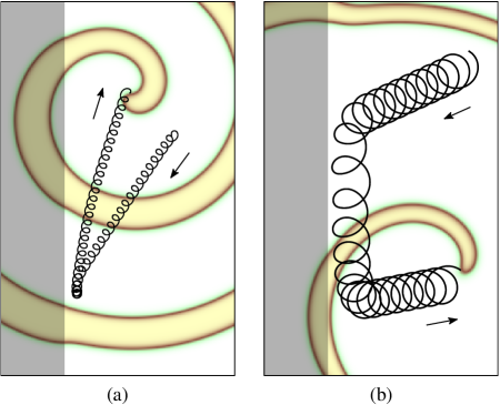
Figure 1: (Color online) Two examples of resonantly drifting spirals reflecting in the Barkley model of a generic excitable medium. The trajectories of the wave tips are drawn in black. Arrows indicate the overall direction of drift. The spiral waves at the final point in the plotted trajectory are visualized by the $u$-field of the Barkley model. Both plots use the same length scale. The boundaries are generated by a step change in medium properties, indicated by gray shading at the left-hand edges. (a) A ‘small-core’ spiral wave approaches a boundary and doubles back on itself; its reflection angle lies on the same side of the boundary normal as its incidence angle. (b) A ‘large-core’ spiral wave speeds up close to the boundary and travels alongside it for a short while before reflecting sharply away. (The plots were cropped to $25\times 40$ space units from simulations performed on a $50\times 50$ square domain, discretized in space with grid spacing $h=1/12$ and in time with time step $\triangle t=2.09\times 10^{-3}$. The step change was located $12$ space units from the left-hand domain wall. Parameters: (a) $a=0.8,b=0.05,c=0.02,\epsilon_{s}=0.035,\epsilon_{f}=1.44\times 10^{-3},\omega_{f}=1.7893$; (b) $a=0.6,b=0.07,c=0.02,\epsilon_{s}=0.035,\epsilon_{f}=4.4\times 10^{-4},\omega_{f}=0.9504$. Details concerning these parameters and the methods used are given in Sec. III.)

Reflections are in general nonspecular: the incidence angle rarely equals the reflection angle. Furthermore, the character of individual reflection trajectories depends on the medium in which the wave propagates, the properties of the boundary and the spiral’s resonant drift velocity.

Numerical simulations of resonantly drifting spiral reflections were undertaken some time ago by Biktashev and Holden Biktashev and Holden (1993), who laid the foundations of the asymptotic approach in a subsequent study Biktashev and Holden (1995). Their numerical work has recently been updated with more extensive simulations and the calculation of a large catalog of reflection trajectories Langham and Barkley (2013). A key feature of spiral wave reflections in these two studies is that the angle of reflection is essentially independent of the angle of incidence for a large range of incident angles. Indeed, the reflection angle instead depends more strongly on the characteristics of the medium than on incident angle. This was predicted by Biktashev and Holden using an ordinary differential equation (ODE) model based on the simplifying assumption that the component of the spiral’s drift velocity caused by interaction with the boundary decays exponentially with distance from the boundary Biktashev and Holden (1993, 1995). However, a more detailed theoretical treatment is required to fully understand the mechanism behind spiral reflection. While separate theoretical accounts of both resonant drift Biktashev and Holden (1993, 1995); Biktasheva et al. (1999, 2010); Xu et al. (2012) and spatial medium inhomogeneities Ermakova and Pertsov (1986); Aranson et al. (1995); Biktasheva (2000); Xu et al. (2009); Biktasheva et al. (2010) (which may act as boundaries to drift) already exist, it is the combination and interaction of these two phenomena which we must consider here.

A good candidate for an updated approach is to use the theory of response functions Biktashev and Holden (1995); Biktasheva et al. (1999); Biktasheva (2000); Biktasheva and Biktashev (2003); Biktasheva et al. (2006, 2009, 2010) which has developed and matured in the years since the Biktashev-Holden study. Response functions are adjoint modes to the neutral symmetry modes of a spiral which characterize how the position and rotation phase of a spiral react to asymptotically small perturbations. In practical terms, response functions allow us to reduce the partial differential equations (PDEs) governing the whole medium to the dynamics of just three real variables—the two spatial coordinates of the wave rotation center and the rotational phase.

In this paper we bring the reflection of drifting spirals into this asymptotic framework by considering the superposition of two small perturbations: one corresponding to resonant forcing generating drift and the other corresponding to a step change in a medium parameter acting as a boundary to drift. Previous studies addressed both effects independently using response functions Biktasheva et al. (1999, 2010). While the approach is strictly applicable only in the limit of slow resonant drift and weak boundary effects, we show that it nevertheless can capture, and thereby explain, most of the important features of spiral wave reflections outside of this asymptotic limit.

II Theory

The underlying dynamics of the excitable medium are well described by models in the class of reaction-diffusion PDEs on the plane:

$$\partial_{t}\mathbf{u}=\mathbf{D}\nabla^{2}\mathbf{u}+\mathbf{f}(\mathbf{u},\mathbf{p})$$ (1)

where $\mathbf{u}(\mathbf{x},t)\in\mathbb{R}^{\ell}$ is a vector of $\ell\geq 2$ state variables for the medium, $\mathbf{f}(\mathbf{u},\mathbf{p})\in\mathbb{R}^{\ell}$ describes the excitable dynamics at each point in space dependent on a vector of $m$ parameters $\mathbf{p}\in\mathbb{R}^{m}$ and $\mathbf{D}\in\mathbb{R}^{\ell\times\ell}$ is a (symmetric) diffusion matrix.

We are interested in models that admit solutions rotating with angular frequency $\omega$ about a center point $R=(X,Y)$. That is, rigidly rotating waves of the form

$$\mathbf{u}=\mathbf{U}(\rho,\vartheta+\omega t-\Phi)$$ (2)

where $(\rho,\vartheta)$ are polar coordinates centered at $R$ and $\Phi$ is the fiducial phase of the spiral at $t=0$. Note that due to symmetries of the plane, if Eq. (1) admits a solution of the form in Eq. (2), then there are infinitely many such solutions related by symmetry, and this is captured by the fact that $R$ and $\Phi$ are arbitrary constants. We refer to $\omega$ as the natural frequency since it is an intrinsic property of the medium, whereas $R$ and $\Phi$ depend on initial data.

Suppose we perturb the medium slightly. In the limit of weak perturbations, this induces small shifts in the rotation center $R$ and the phase $\Phi$, leaving the shape of the spiral otherwise unchanged. Thus the response of the spiral to weak perturbations is a trajectory through the space of solutions of the form Eq. (2), where $R$ and $\Phi$ depend on time.

Mathematically, we treat such a perturbation as the addition of a vector $||\epsilon\mathbf{h}(\mathbf{x},t)||\ll 1$ to the right-hand side of Eq. (1). It can be shown using perturbation methods Biktashev and Holden (1995); Biktasheva et al. (1999, 2006) that to first order in $\epsilon$, the time derivatives of $R(t)$ and $\Phi(t)$ are proportional to the $L^{2}$ inner products $\langle\cdot,\cdot\rangle$ of the spiral’s response functions $\mathbf{W}_{0}$ and $\mathbf{W}_{1}$ with the perturbation vector, averaged over one full rotation period $T=2\pi/\omega$:

$$\dot{\Phi}(t) =\frac{\epsilon}{T}\int_{t-T/2}^{t+T/2}\left\langle\mathbf{W}_{0},\mathbf{h}\right\rangle d\tau+O(\epsilon^{2})$$ (3)

$$\dot{R}(t) =\frac{\epsilon}{T}\int_{t-T/2}^{t+T/2}e^{i(\Phi-\omega\tau)}\left\langle\mathbf{W}_{1},\mathbf{h}\right\rangle d\tau+O(\epsilon^{2})$$ (4)

where we use the identification $R=(X,Y)\equiv X+iY$.

Technical details can be found in the appendix and elsewhere Biktashev and Holden (1995); Biktasheva et al. (1999); Biktasheva and Biktashev (2003); Biktasheva et al. (2006, 2009, 2010), but the essence of these equations is the following. The response functions are adjoint fields corresponding to the symmetries of the reaction-diffusion system [Eq. (1)]. $\mathbf{W}_{0}$ is $\mathbb{R}^{\ell}$-valued and corresponds to the presence of rotational symmetry. One can think of the perturbation, $\epsilon\mathbf{h}$, as providing an infinitesimal impulse $\epsilon\left\langle\mathbf{W}_{0},\mathbf{h}\right\rangle$ along the direction of the symmetry (phase $\Phi$ in this case), at each time $\tau$. Equation (3) captures the effect of all such impulses over one rotation period to give the rate of change in $\Phi$.

The response function $\mathbf{W}_{1}$ is $\mathbb{C}^{\ell}$-valued and corresponds to the two translational symmetries. Here the perturbation at each time $\tau$ provides the spiral with an infinitesimal impulse in the direction $\arg{\langle\mathbf{W}_{1},\mathbf{h}\rangle}$ rotated by $e^{i(\Phi-\omega\tau)}$ due to the underlying natural rotation of the spiral. These contributions, averaged over one rotation period, give the drift velocity. Importantly, a change in $\Phi$ typically implies a change in the direction of drift.

Response functions have been computed numerically for a variety of spiral waves in previous studies. For various cases, including that of the spiral waves we study here, the support of these functions was found to be highly localized around the spiral rotation center Biktasheva and Biktashev (2003); Biktasheva et al. (2006, 2010). Thus, a spiral wave drifts only in response to perturbations very close to the core. That is, it behaves as a particle whose position may be identified with the rotation center $R$.

We are interested in the case where a resonantly forced spiral moves towards, and reflects from, a boundary in the medium. This is a combination of two perturbations to the original reaction-diffusion equations—a homogeneous, time-periodic one that causes resonant drift of the spiral and a spatial one that imposes a boundary to the drifting spiral. Let us suppose the resonant forcing can be described by some $\mathbf{h}_{f}(t)$. In practice we will consider the simple case of harmonic forcing of one of the medium parameters at the natural frequency $\omega$. Likewise, suppose that the effect of a boundary may be formulated in $\mathbf{h}_{s}(\mathbf{x})$. The type of boundary we shall consider is a sharp interface along the line $x=0$ between two media with different excitability properties. Although this is not a physical barrier to wave propagation, a drifting spiral core may nevertheless reflect from the spatial inhomogeneity; see Fig. 1 and Ref. Langham and Barkley (2013). We refer to this as a step boundary. It may be considered as a weak perturbation provided that the step change in medium parameters is small. In previous studies a Neumann or ‘no-flux’ boundary was also considered. While this type of boundary condition cannot be treated as a weak perturbation, it has previously been observed that reflections from a step inhomogeneity are qualitatively similar to the no-flux case Langham and Barkley (2013).

The total perturbation to the medium can be written as $\mathbf{h}(\mathbf{x},t)=\epsilon_{s}\mathbf{h}_{s}(\mathbf{x})+\epsilon_{f}\mathbf{h}_{f}(t)$, where $0<\epsilon_{s},\epsilon_{f}\ll 1$ represent the strengths of the respective ‘step’ and ‘forcing’ perturbations. One can immediately see from Eqs. (3) and (4) that the effects of the two perturbations on $\dot{\Phi}$ and $\dot{R}$ are a linear superposition and may therefore be considered separately. It may consequently be shown (see the appendix) that the equations of motion for the spiral center $R=(X,Y)$ and phase $\Phi$ are of the form

$$\dot{X} =\epsilon_{s}S_{X}(X)+\epsilon_{f}F_{X}(\Phi)$$ (5)

$$\dot{Y} =\epsilon_{s}S_{Y}(X)+\epsilon_{f}F_{Y}(\Phi)$$ (6)

$$\dot{\Phi} =\epsilon_{s}S_{\Phi}(X)$$ (7)

where $S_{X}$, $S_{Y}$, $S_{\Phi}$ are contributions due to the step boundary and $F_{X}$, $F_{Y}$ are contributions due to the resonant forcing. These are given by integrals of the form in Eqs. (3) and (4). While the functions depend in detail on the specific model used and the particular spiral wave under consideration, their general form, in particular their respective dependence on $X$ and $\Phi$ as indicated, is independent of these details.

Since the step boundary is located along the line $x=0$ in the original PDE, the dynamics of the spiral depends only on the distance $X$ of the spiral center from step boundary and does not depend on $Y$. Likewise, since the step perturbation is time independent, its effect, when averaged over a full spiral rotation, cannot depend on the spiral’s phase $\Phi$.

The form of the functions $F_{X}$ and $F_{Y}$ and the role of $\Phi$ are quite important. In the appendix we show that for sinusoidal resonant forcing of a medium parameter:

$$F(\Phi)=Ae^{i\Phi}$$ (8)

where $F\equiv F_{X}+iF_{Y}$ and $A$ is a real constant for each model and set of parameter choices. Hence, for a given spiral wave and given forcing amplitude, the drift velocity due to resonant forcing is, in the asymptotic limit, constant with direction determined by the phase $\Phi$. This direction of drift can change as a result of interaction with the boundary, i.e., the function $S_{\Phi}$, but not due to periodic forcing alone.

Equations (5), (6) and (7) reduce the spiral dynamics from a set of nonlinear PDEs to three coupled autonomous nonlinear ODEs. The functions $S_{X}$, $S_{Y}$, $S_{\Phi}$, $F_{X}$, and $F_{Y}$ on the right-hand sides must in practice be obtained numerically by taking appropriate inner products with numerically computed response functions. Nevertheless, evaluating the right-hand sides and then numerically solving the ODEs can be done quickly with minimal computational resources. It is worth noting that the essential dynamical quantities $X$, $Y$, and $\Phi$ are the same variables that Biktashev and Holden used in their asymptotic theory of spiral reflections Biktashev and Holden (1993, 1995). Moreover, we stress that while the variable $\Phi$ was introduced as the phase of the spiral wave, its role in the reduced system becomes the direction of drift due to periodic forcing.

III Model and Methods

The previous discussion of response functions did not depend on any specific model. Here, we consider spiral wave solutions in the standard Barkley model Barkley (1991, 2008), for which $\ell=2$:

$$\frac{\partial u}{\partial t}=\nabla^{2}u+\frac{1}{c}u(1-u)\left(u-\frac{v+b}{a}\right),$$ (9)

$$\frac{\partial v}{\partial t}=u-v.$$ (10)

The two state variables $u(x,y,t)$ and $v(x,y,t)$ capture, respectively, the excitation and recovery processes of the medium. Parameters $a,b>0$ control the threshold for excitation and $0<c\ll 1$ sets the timescale of the fast excitation process, relative to recovery. (The parameter $c$ is usually called $\epsilon$ but we will not use that notation here.) For fixed parameter $c$ and variable $a,b$, the section of parameter space which admits rigidly rotating spiral wave solutions is divided roughly into two regimes distinguished by the size of the rotation core. The reflective properties of so-called small- and large-core spirals markedly differ Langham and Barkley (2013) and we therefore divide our study along these lines.

Throughout our study we have varied the $b$ parameter to create the step inhomogeneity by considering $b(x)=b_{0}+\epsilon_{s}(H(x)-1)$, where $H$ is the Heaviside step function. Resonant forcing has been applied homogeneously by varying the excitability $c$ as $c(t)=c_{0}+\epsilon_{f}\cos(\omega_{f}(t-t_{0}))$, where $\omega_{f}$ is the forcing frequency required to obtain resonant drift and $t_{0}$ is some initial forcing time (the choice of which is discussed in the appendix). For our results in Sec. IV, $\omega_{f}=\omega$. In all numerical simulations, the values of $\epsilon_{s}$ and $\epsilon_{f}$ have been chosen small enough that the perturbed medium remains in the same parameter regime (of small- or large-core rigid rotation) as the unperturbed parameters.

The response functions and natural rotation frequencies for various small- and large-core spirals in the Barkley model were calculated on a polar grid using the software DXSpiral Barkley et al. (2010). The numerical methods are detailed in Ref. Biktasheva et al. (2009). A disk of radius $15$ was used in the small core with $64$ angular grid points and $1875$ radial grid points. In the large core the radius size was increased to $20$ and the number of radial grid points used was $2500$. The resulting response function discretizations were used to numerically compute the right-hand sides of Eqs. (5), (6), and (7) (see the appendix for the specific integrals), again using DXSpiral. Reflection trajectories were calculated by timestepping the resulting three dynamical variables from chosen initial conditions.

Direct numerical simulations of the Barkley model PDEs were also performed for comparison with the response function predictions. These were computed using the standard finite-difference techniques described in Refs. Barkley (1991); Dowle et al. (1997). These simulations use unusually high precision to ensure that they correctly capture the spiral rotation frequency (Biktasheva et al., 2010, Sec. IV B). (The simulations involve forcing at the natural frequency, i.e. $\omega_{f}=\omega$, obtained very accurately from DXSpiral. Small inaccuracies in the simulations, which would normally be irrelevant, result in artificial frequency mismatches which then lead to artificially curved trajectories.) In the small core (Fig. 12) a $20\times 20$ square domain was used with grid spacing $h=0.0125$ and time step $\triangle t=2.3\times 10^{-5}$. The step inhomogeneity was located $5$ space units from the left-hand domain edge. In the large core (Fig. 13) a larger $40\times 40$ square domain was used, with the step inhomogeneity located $10$ space units from the left-hand edge, in order to avoid interaction of the spiral wave with the no-flux domain walls. The grid spacing was $h=0.025$, with corresponding time step $\triangle t=9.4\times 10^{-5}$. Model parameter values are given later in the text.

IV Results

Before presenting our response function calculations, we make a note concerning incident and reflected angles. As is standard, we define both the angles of incidence $\theta_{i}$ and reflection $\theta_{r}$ to be measured from the boundary normal. In the case of light paths in classical optics, one considers incident angles only in the range $[0^{\circ},90^{\circ}]$, since, due to symmetry in the $y$-direction, trajectories at equal angles either side of the normal correspond to physically identical situations. However, since spirals possess a chirality, this symmetry is not present and we must consider both incident and reflected angles in the range $[-90^{\circ},90^{\circ}]$.

In Sec. II and the appendix we have implicitly set $\omega>0$ to correspond to clockwise rotation. We consider spirals of this chirality only. Our convention is to define $\theta_{i}$ to be positive in the clockwise direction from the normal and $\theta_{r}$ to be positive in the counterclockwise direction from the normal. That is, incident and reflected angles on opposite sides of the normal have the same sign.

IV.1 Small-core case

Our study begins by considering spiral waves in the small-core region of parameter space. We set $a=0.8$, $b=0.05$, and $c=0.02$. Figure 2 shows the step boundary functions $S_{X}$, $S_{Y}$, and $S_{\Phi}$ for these parameters.

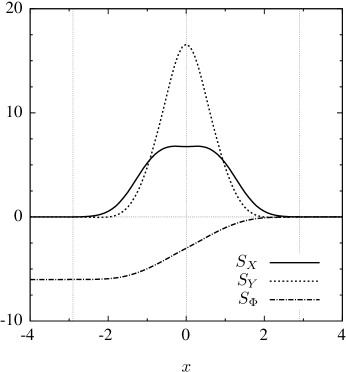
Figure 2: $S_{X}$, $S_{Y}$, and $S_{\Phi}$ for a small-core spiral with $a=0.8$, $b=0.05$, and $c=0.02$. Also plotted in dotted gray are the vertical lines $x=\pm 2.9$, which enclose the effective boundary region. [For $|x|>2.9$, $S_{X}(x)$ and $S_{Y}(x)$ are less than 0.1% of $S_{X}(0)$ and $S_{Y}(0)$ respectively.]

These curves represent the intrinsic character of the boundary influence. Let us first consider the effects of this boundary in the absence of resonant forcing. The dynamics of the spiral rotation center in this case are governed simply by the $S_{X}$ and $S_{Y}$ curves, scaled by the size of the step:

$$\dot{R}=\epsilon_{s}S(X)$$ (11)

where $S\equiv S_{X}+iS_{Y}$. We see, as expected, that $S_{X}$ and $S_{Y}$ are zero outside a relatively small neighborhood of $x=0$ and thus spirals outside this region are unaffected by the step boundary. Since $S_{X}(X)$ is positive inside the boundary region, spirals to the right of $x=0$ are repelled away from the step.

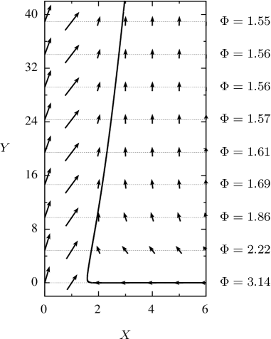
Figure 3: Theoretical trajectory of a small-core spiral wave reflection with $\theta_{i}=0^{\circ}$ and $\epsilon_{f}/\epsilon_{s}=1/25$. Initial conditions: $X_{0}=6$, $Y_{0}=0$, $\Phi_{0}=\pi$. Each horizontal row of vectors plots the velocity field at the instant at which the spiral center attained the given $Y$. These vectors depend on $X$ and the phase $\Phi$. The value of $\Phi$ at each horizontal slice is indicated on the right-hand side. Vector magnitudes have been scaled nonlinearly for visual clarity. The ratio of the $X:Y$ scales is $1:4$.

Furthermore, since $S_{Y}(X)$ is also positive in this region, the boundary acts to intrinsically drive spirals in the positive $y$-direction. Note also the antisymmetry of $S_{\Phi}$. Far to the left of the boundary, $S_{\Phi}(X)$ tends to a non-zero (negative in this case) constant. This is because the spiral’s rotation frequency in the left half-plane, with the perturbed model parameter $b_{0}-\epsilon_{s}$, differs from the ‘natural’ frequency $\omega$ of the unperturbed spiral in the right half-plane.

Now let us add in the effect of periodic forcing. The rotation center in this case moves according to

$$\dot{R}=\epsilon_{s}S(X)+\epsilon_{f}F(\Phi)$$ (12)

where $F(\Phi)=Ae^{i\Phi}$, from Eq. (8). Thus, the velocity at each instant is the superposition of the step component and a vector of fixed magnitude due to the resonant forcing, whose direction is set by the spiral’s phase $\Phi$. Far from the boundary, the velocity is constant, since $S(X)=0$ and $S_{\Phi}(X)=0$ for $X\gg 0$. Close to the boundary, if the step perturbation is large enough relative to the resonant forcing perturbation, the boundary effects dominate and spirals in the positive half-plane are repelled from the step. Furthermore, since $S_{\Phi}(X)<0$ for $X\lesssim 2.9$, the forcing component rotates clockwise in time while the spiral is in the boundary region.

Figure 4: Two theoretical trajectories in the small-core regime, initiated at $X_{0}=6$, $Y_{0}=0$. $\epsilon_{f}/\epsilon_{s}=1/25$. The filled points plotted along the trajectories are equally spaced in time to indicate drift speed. Incident angles are (a) $\theta_{i}\approx-70^{\circ}$ and (b) $\theta_{i}\approx+70^{\circ}$. Both spirals reflect with angle $\theta_{r}\approx+88^{\circ}$. The ratio of the $X:Y$ scales is $1:1$.

This suggests a mechanism for reflection. Consider a resonantly forced spiral wave traveling towards the step from the right half-plane. Far from the boundary, the spiral drifts with constant velocity at some incident angle $\theta_{i}$ (set by initial conditions). On entering the boundary region, the spiral is repelled by the inhomogeneity, causing it to slow and preventing it from passing through $x=0$. This effect itself does not cause the subsequent reflection from the boundary. The motion away from the boundary is rather due to the $\Phi$ dynamics. As the spiral approaches the boundary, $\Phi$ decreases bringing about a rotation in the resonant forcing component $F(\Phi)$. After a time, this component inevitably rotates around to the positive $x$-direction and this drives the spiral away from the step. Consequently, the spiral leaves the boundary at some reflection angle $\theta_{r}$, dictated by the phase on exiting the boundary region.

We see this mechanism at work in Fig. 3, which displays a typical theoretical reflection trajectory in the small-core regime. (One should note that the lengths of vectors in Fig. 3 have been scaled nonlinearly so their directions far from the step are discernable—the magnitude of the forcing component is comparatively much weaker than depicted.)

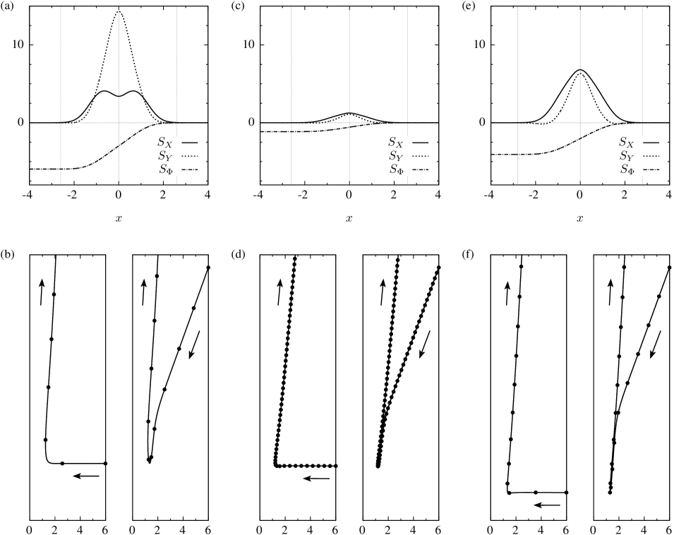
Figure 5: $S_{X}$, $S_{Y}$, and $S_{\Phi}$ curves, together with representative theoretical reflection trajectories for three different small-core spiral waves. $\epsilon_{f}/\epsilon_{s}=1/50$. Each pair of reflection trajectories is plotted below the corresponding boundary curves. The left- and right-hand trajectories are $\theta_{i}\approx 0^{\circ}$ and $\theta_{i}\approx-70^{\circ}$, respectively, and include filled points, matched to the timestep of the corresponding points in Fig. 4, indicating drift speed. Model parameters: in (a) and (b) $a=0.7$, $b=0.01$; in (c) and (d) $a=0.95$, $b=0.01$; in (e) and (f) $a=0.95$, $b=0.08$. In all cases $c=0.02$. These span a substantial extent of the small-core regime.

After entering the boundary region, the spiral undergoes a rapid change in direction and phase and its speed in the $x$-direction slows considerably. As the resonant forcing component $F(\Phi)$ (depicted in the rightmost vectors of Fig. 3) rotates with the decreasing phase, its $x$-component diminishes and consequently the boundary effects push the spiral center further away from the step. This process is slow and the spiral travels far in the $y$-direction in this time. Eventually, the evolving phase turns the resonant drift direction towards the positive half-plane, i.e., $F_{X}(\Phi)$ changes sign and becomes positive. As a result, the spiral center leaves the boundary. The reflected angle is close to $+90^{\circ}$, since $S_{\Phi}(X)$ is very near zero when this sign change occurs and therefore phase changes only by a small amount after this.

We observe that the situation is similar across the full range of incident angles $\theta_{i}\in[-90^{\circ},90^{\circ}]$. Figure 4 displays two theoretical reflection trajectories which approach the boundary at different angles, either side of the normal, reflecting in the same direction. Regardless of incident angle, the spiral center may only leave the boundary once $F(\Phi)$ points away from the step. Each spiral wave reaches this sign change of $F_{X}(\Phi)$ in essentially the same state: with $\Phi=\pi/2$ and $X$ close to the edge of the boundary region. This is because the $\Phi$ dynamics are sufficiently slow that the spiral center is pushed almost completely out of the boundary region by the time that $\Phi=\pi/2$. Therefore each spiral wave changes direction by only a small amount after this point and reflects with $\theta_{r}$ close to $+90^{\circ}$.

It is worth noting that in addition to the invariance of reflection angle, these theoretical trajectories exhibit qualitative features observed in numerical simulations. In particular, the nontrivial shape of Fig. 4(a), the sharp change of direction at the boundary in Fig. 3 and the decrease in the closest distance to the boundary reached by the spiral center as $\theta_{i}$ increases. For comparison see Figs. 3(b), 4(g) and 4(h) in Ref. Langham and Barkley (2013).

Across the small-core parameter regime, we see that the curves $S_{X}$, $S_{Y}$, and $S_{\Phi}$ vary in magnitude and shape. However, the qualitative differences in the theoretical reflection trajectories are only subtle and the reflection mechanism in each case is the same. Representative curves and trajectories are plotted in Fig. 5.

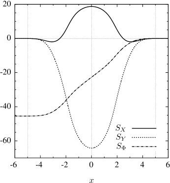
Figure 6: $S_{X}$, $S_{Y}$ and $S_{\Phi}$ for a large-core spiral with $a=0.6$, $b=0.07$, $c=0.02$. Also plotted in dotted gray are the vertical lines $x=\pm 5.0$, which enclose the effective boundary region. [For $|x|>5.0$, $|S_{X}(x)|$ and $|S_{Y}(x)|$ are less than 0.1% of $S_{X}(0)$ and $S_{Y}(0)$ respectively.]

IV.2 Large-core case

We now turn to the large-core case, setting $a=0.6$, $b=0.07$, and $c=0.02$. As before, we begin by plotting the $x$-dependence of the key functions $S_{X}$, $S_{Y}$, and $S_{\Phi}$, shown in Fig. 6. At first glance these do not appear differ too much from the corresponding curves in the small core (see Figs. 2 and 5). Nevertheless, there are differences, some of which are quite important. The region of boundary influence is wider than in the small-core, extending to roughly a distance of five space units from the step inhomogeneity. This is expected: spiral waves propagate outwards from their tips, which rotate around a circle of much larger radius in the large-core. Furthermore, $S_{X}$ has roots within this boundary region, at $x\approx\pm 2.5$. The root at positive $x$ is attracting (in the absence of resonant forcing). Also, the magnitudes of the curves are (pointwise) greater than those in the small-core case. For the set of parameters we consider, this is particularly true for $S_{\Phi}$. Finally, notice that $S_{Y}$ has changed sign with respect to the small-core case.

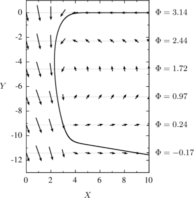
Figure 7: Theoretical trajectory of a large-core spiral reflection with $\theta_{i}=0^{\circ}$ and $\epsilon_{f}/\epsilon_{s}=1/87.5$. Initial conditions: $X_{0}=10$, $Y_{0}=0$, $\Phi_{0}=\pi$. Each horizontal row of vectors plots the velocity field at the instant at which the spiral center attained the given $Y$. These vectors depend on $X$ and the phase $\Phi$. The value of $\Phi$ at each horizontal slice is indicated on the right-hand side. Vector magnitudes have been scaled nonlinearly for visual clarity. The ratio of the $X:Y$ axes is $1:1$.

These differences have a significant impact on the character of reflections for spiral waves in the large-core region. Figure 7 demonstrates a typical theoretical trajectory. Approaching at $\theta_{i}=0^{\circ}$, the spiral changes direction as it enters the boundary region as before, but turns to move in the negative rather than the positive $y$-direction, since $S_{Y}$ is large and negative inside the boundary region. While $\pi/2<\Phi<\pi$, the resonant forcing has negative $x$-component and the spiral remains near the positive root of $S_{X}$. Once $\Phi$ decreases to less than $\pi/2$, the forcing acts to push the spiral away from the boundary. As it exits, $\Phi$ continues to decrease causing the resonant forcing direction to turn further clockwise. Finally, the spiral leaves the boundary at the constant angle dictated by $\Phi=-0.17$ ($\theta_{r}\approx-9.5$ in this case). Qualitatively similar trajectories for low amplitude resonant forcing in the large core have been observed previously for Neumann boundary conditions; see Fig. 10(c) of Ref. Langham and Barkley (2013).

The key difference between this large-core case and the small-core theoretical trajectories in Sec. IV.1 is the attracting root of the $S_{X}$ curve, which importantly occurs within the boundary region.

Figure 8: Effect of incident angle $\theta_{i}$ for a large-core spiral. Various theoretical trajectories are shown with different initial $\Phi_{0}$ and $\epsilon_{f}/\epsilon_{s}=1/87.5$. The filled points plotted along the trajectories are equally spaced in time to indicate drift speed. Incident angles: (a) $\theta_{i}=60^{\circ}$, (b) $\theta_{i}=67.5^{\circ}$, (c) $\theta_{i}=75^{\circ}$.

While the spiral is in the boundary region, the phase evolves, causing the resonant forcing component to rotate, just as with small-core spirals. Once $F_{X}(\Phi)$ changes sign, the resonant forcing turns to impel the spiral away from the boundary. While in the small-core cases this occurs when the spiral center is near to the end of the boundary region, in the large-core case the spiral remains close to the attracting root of $S_{X}$ prior to the sign change. Since the magnitude of $S_{\Phi}$ is non-negligible near the attracting root of $S_{X}$, $\Phi$ continuous to evolve, decreasing for some time as the spiral exits the boundary. Consequently, the final direction of the spiral differs greatly from $+90^{\circ}$.

In the large-core regime, we see a notable effect of incident angle on reflection angle. Using the same parameters, we demonstrate this in Fig. 8. Spirals approaching the boundary at higher incidence angles have lower initial phase and consequently reach the sign change of $F_{X}(\Phi)$ (at $\Phi=\pi/2$) sooner. Therefore, at high incident angles the sign change occurs much further from the step than at low incident angles, since $\Phi$ reaches $\pi/2$ before the spiral center reaches the attracting root of $S_{X}$. This means these spirals necessarily leave the boundary region sooner and with a greater $\Phi$, i.e., greater reflected angle. This can be visualized more clearly by plotting the trajectory of the phase with respect to the distance from the boundary, as we have done in Fig. 9.

The change in sign of the $S_{Y}$ curve between the large- and small-core parameter regimes has no effect on reflection angle, since the dynamics of the spiral center far from the boundary depends only on $\Phi$ and $X$.

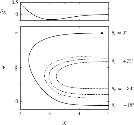
Figure 9: Phase dynamics for large-core spirals approaching the boundary with different incident angles. $\epsilon_{f}/\epsilon_{s}=1/87.5$. The top plot shows the curve $S_{X}$, for reference. The bottom plot shows the theoretical ‘trajectory’ of the spiral phase as the spiral moves in and out of the boundary region, for various incident angles. Incoming trajectories have $\Phi\in(\pi/2,3\pi/2)$ and outgoing trajectories have $\Phi\in(-\pi/2,\pi/2)$. The solid black trajectory corresponds to the reflection in Fig. 7 and the dotted and dashed trajectories correspond to the reflections in Fig. 8.

However, it is relevant to the overall qualitative shape of trajectories at the boundary. This difference in sign can be qualitatively explained by referring to arguments given by Krinsky et al. Krinsky et al. (1996) for the case of spiral wave drift in electric fields, which were later studied by Xu et al. Xu et al. (2009) for medium inhomogeneities. Drift of the spiral rotation center may be caused by changes to the radius of the rotation core and also by changes to the rotation frequency. In the Barkley model, decreasing the $b$ parameter, as we have done to form the step boundary, decreases the core size and increases the rotation frequency. The effect of our step inhomogeneity on the core radius causes the spiral to drift in the negative $y$-direction. However, the effect on the rotation frequency causes the spiral to drift in the positive $y$-direction. For small-core parameters, the core radius changes little and the effect of the step boundary on the rotation frequency dominates. In the large-core parameter region, it is instead the changes in the core radius which dominate. Therefore the vertical component of drift due to the boundary changes sign between the two parameter regions.

Figure 10: Effect of forcing amplitude on large-core spiral waves. Three theoretical trajectories are shown in order of increasing amplitude and include filled points, matched to the timestep of the corresponding points in Fig. 8, indicating drift speed. The perturbation ratio $\epsilon_{f}/\epsilon_{s}$ in each case equals (a) $1/75$, (b) $1/50$, and (c) $1/25$.

We may also consider the effects of altering the ratio $\epsilon_{f}/\epsilon_{s}$. Let us fix $\epsilon_{s}$ and vary $\epsilon_{f}$. Higher $\epsilon_{f}$ corresponds to higher amplitude resonant forcing, meaning that the drift speed due to resonant forcing is greater. Figure 10 plots some illustrative theoretical reflection trajectories at different amplitudes.

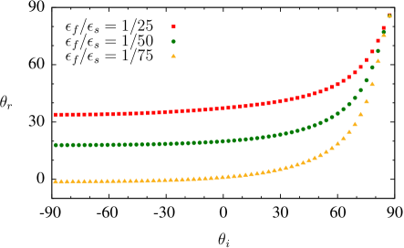
Figure 11: (Color online) Reflected angle $\theta_{r}$ versus incident angle $\theta_{i}$ for large-core spirals at different forcing amplitudes. The angles were measured from the theoretical response function trajectories at the given $\epsilon_{f}/\epsilon_{s}$ ratios.

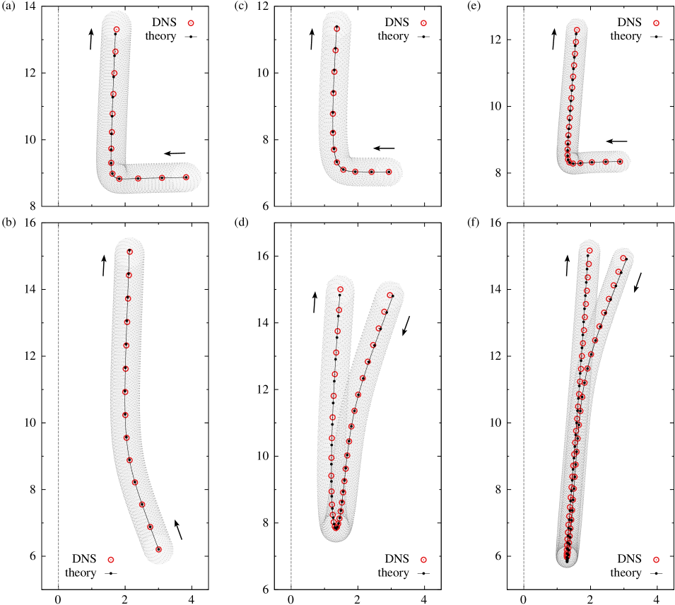
Figure 12: (Color online) Comparison between theory and direct numerical simulation (DNS) of the Barkley model for a variety of parameter values and incident angles in the small-core regime. In each case the rotation center of the spiral wave in the DNS is plotted (open circles) every 30th rotation period. The theoretical trajectories (curves with solid dots) use an initial condition selected such that they agree with the DNS trajectory at a point close to the boundary. Solid dots are separated by a time corresponding to 30 rotation periods. Also shown are the rotating spiral tip trajectories, dotted in gray, and the step boundary at $x=0$, dashed in gray. Each of the three columns corresponds to a different choice of model parameters broadly spanning the small-core parameter regime. Within each column two incident angles are shown: one normal and one oblique to the boundary. Parameters in (a) and (b): $a=0.8$, $b=0.05$, $c=0.02$, $\omega_{f}=1.850564$, $\epsilon_{f}/\epsilon_{s}=4\times 10^{-5}/3.5\times 10^{-3}=1/87.5$; in (c) and (d): $a=0.7$, $b=0.01$, $c=0.02$, $\omega_{f}=2.043489$, $\epsilon_{f}/\epsilon_{s}=4\times 10^{-5}/2\times 10^{-3}=1/50$; in (e) and (f): $a=0.95$, $b=0.08$, $c=0.02$, $\omega_{f}=1.768359$, $\epsilon_{f}/\epsilon_{s}=4\times 10^{-5}/2\times 10^{-3}=1/50$.

We see that as resonant forcing amplitude increases, reflected angle increases. This is because higher amplitude forcing impels spirals with greater drift speed. Faster spirals leave the boundary more quickly after $F_{X}(\Phi)$ changes sign and therefore leave with a greater $\Phi$. (Note that they also approach closer to the step, which acts to decrease reflection angle, but this effect is not significant relative to the effect of increased drift speed.)

The combined effects of incidence angle and forcing amplitude are illustrated in Fig. 11, where we plot reflected angle $\theta_{r}$ versus incident angle $\theta_{i}$ for the three forcing amplitudes used in Fig. 10. These theoretical incidence-reflection data are qualitatively close to previously reported large-core results from direct numerical simulation (albeit with Neumann boundary conditions): see Fig. 9 of Ref. Langham and Barkley (2013).

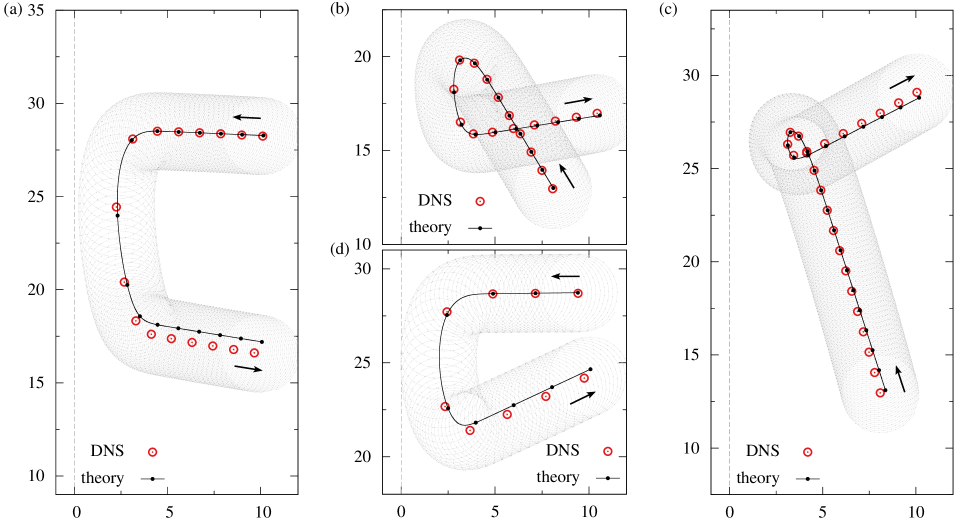
Figure 13: (Color online) Comparison between theory and direct numerical simulation (DNS) of the Barkley model in the large-core regime verifying the theoretical predictions for the role of incident angle and forcing amplitude. Plot (a) shows a simulation of the case explained theoretically in Fig. 7, in which $\theta_{i}\approx 0^{\circ}$. Between (a), (b) and (c), the incident angle was varied from $0^{\circ}$ to approximately $60^{\circ}$ and $70^{\circ}$, respectively, keeping all other parameters fixed. In (d), the resonant forcing perturbation used was twice that of (a), while the incident angle and all other parameters remained fixed. Thus the effects of incident angle and forcing amplitude are seen to agree with those predicted in Figs. 8 and 10 and explained theoretically in Sec. IV.2. In each case the rotation center of the spiral in the DNS is plotted (open circles) every 10th rotation period. The theoretical trajectories (curves with solid dots) use an initial condition selected such that they agree with the DNS trajectory at a point close to the boundary and are plotted with a time step (time between successive points) corresponding to 10 rotation periods of the simulation. Also shown are the rotating spiral tip trajectories, dotted in gray, and the step boundary at $x=0$, dashed in gray. Parameters: $a=0.6$, $b=0.07$, $c=0.02$, and $\omega_{f}=0.9164372$; in (a)–(c) $\epsilon_{f}/\epsilon_{s}=4\times 10^{-5}/3.5\times 10^{-3}=1/87.5$; in (d) $\epsilon_{f}/\epsilon_{s}=8\times 10^{-5}/3.5\times 10^{-3}=1/43.75$.

IV.3 Comparison with direct numerical simulation

Figures 12 and 13 show comparisons between the reflection trajectory predicted by our response function calculations and results from direct numerical simulation (DNS) of the full Barkley model PDEs using the same parameters. A thorough study of the numerical convergence of the asymptotic theory in the separate cases of resonant parameter forcing and step inhomogeneity has previously been conducted Biktasheva et al. (2010) and consequently we do not repeat such a study here. Instead, the cases presented have been chosen to demonstrate various phenomena predicted theoretically in the preceding sections. Excellent agreement is seen between theory and full DNS of spiral waves over a broad range of parameters and conditions.

In the small-core cases, Fig. 12, the spiral wave drift direction, drift speed, and point of closest approach to the boundary are in very close correspondence with theoretical predictions. Note that speed is gauged from the distance traveled between successive points (open circle for DNS and filled circles for theory). Most of the (very small) differences between DNS and theory arise in the vicinity of the boundary where the effects of both perturbations are felt. Since points are plotted at fixed time intervals over the full trajectory, small speed differences can nevertheless give rise to an accumulated shift between points from DNS and theory. The most striking feature in the small-core regime is the correct theoretical prediction at large negative incident angles: Figs. 12(d) and 12(f). Theory correctly predicts that the spiral center first moves downward near the boundary for a large number of rotation periods before turning, moving upward, and slowly leaving the boundary.

In the case of large-core spiral waves, Fig. 13, the considerable variation in the reflected angle predicted by theory is seen to hold in the full DNS. In particular, for fixed parameter values, as the incident angle is changed from near zero, Fig. 13(a), to large positive angles, Figs. 13(b) and 13(c), the drift trajectory spends less time in the vicinity of the boundary and develops a loop as the reflected angle changes from negative (moving down and to the right in the figure) to positive (moving up and to the right). (See also for comparison Fig. 8.) Furthermore, as the forcing amplitude is increased for otherwise fixed conditions [Fig. 13(a) and Fig. 13(d)], the time at the boundary decreases and the reflection angle increases. (See also for comparison Fig. 10.)

The agreement between asymptotics and DNS is not quite as good in the large-core results, Fig. 13, as in the small-core results, Fig. 12. The main visible difference between theory and DNS in the large core regime is the point at which the spiral center leaves the boundary. Other features, such as the reflected angle and the point of closest approach are predicted well. Discrepancies between theory and DNS are due to slight frequency mismatches. Large-core spiral waves are particularly susceptible to this as their rotation frequencies and tip orbits vary rapidly with parameters Winfree (1991). In the DNS there is a shift from the unperturbed rotation frequency $\omega$ (as calculated to high accuracy by DXSpiral) due to small but finite spatial discretization errors, as well as weak nonlinear effects at finite perturbation strength. As the perturbation magnitudes and the computational grid spacing tend to zero, the theoretical and DNS trajectories do converge Biktasheva et al. (2010).

V Discussion

We have applied the theory of response functions to the reflection of spiral wave trajectories from boundaries. Via numerical computation of response functions, we have studied reflections in the asymptotic limit of slow drift and weak boundary effects. In this limit the approach is quantitatively accurate, as we have demonstrated for a variety of cases by comparing direct simulations of spiral waves in a full reaction-diffusion model with the theoretical predictions from response functions. However, the main value of the response function approach is the qualitative understanding it brings to how interactions with a boundary lead to different types of reflections in various situations. Several of the most significant features of spiral wave reflections, previously observed in simulations at higher drift speeds and greater step inhomogeneities Langham and Barkley (2013), are nevertheless captured qualitatively by the asymptotic analysis. Consequently, we have been able to understand the essential causes of many interesting aspects of spiral wave reflections.

As stated in the Introduction, the primary characteristic of spiral wave reflections is that across a wide range of model parameters, the reflected angle is approximately constant for large ranges of incident angle. This reflection angle ‘plateau’ is present in the response function results in both small- and large-core cases. In the small-core case, it was previously demonstrated numerically that the value of this constant angle increases toward $\theta_{r}=+90^{\circ}$ as the resonant drift velocity decreases Langham and Barkley (2013). Our asymptotic results reveal the limiting case of this trend, yielding only reflected angles very close to $\theta_{r}=+90^{\circ}$ and we have shown exactly why the reflected angle is essentially constant across a wide range of parameter space.

Another significant feature observed in prior numerical simulations of reflections is that, unlike the small-core case, for large-core spirals the reflected angle increases with increasing drift velocity Langham and Barkley (2013). This effect is clearly present in the asymptotics (Figs. 10 and 11) and in the comparison with DNS [Figs. 13(a) and 13(d)]. The qualitative form of the reflection angle data in Fig. 11—a plateau for negative $\theta_{i}$, then monotonically increasing at high $\theta_{i}$—is familiar to all previous numerical results and emerges naturally from the response function model by considering Fig. 9. Furthermore, general consideration of the differences between small- and large-core spiral waves at the asymptotic level has led to explanations of the diversity of behaviors between the two cases. Finally, we note that the non-trivial shape, closest boundary approach distance, and relative drift speeds that are obtained and explained via the response function analysis are all observed qualitatively beyond the asymptotic limit, in both the small- and large-core cases Langham and Barkley (2013).

The work presented in this paper fits comfortably with that which is already known about spiral wave reflections. Biktashev and Holden Biktashev and Holden (1993) recognized many years ago that reflections are caused by small deviations from the natural rotation frequency on close approach to the boundary, which alter the direction of drift. They proposed asymptotic equations of motion for the rotation center and phase, positing that the boundary effects (corresponding to $S_{X}$, $S_{Y}$, and $S_{\Phi}$ in our notation) decay exponentially with distance from the boundary. These simple assumptions ably capture the overriding feature of spiral wave reflections—large ranges of approximately constant reflected angle—but beyond that the predictive qualities of the model are limited. Our application of response functions to the reflection problem can be viewed as an extension of their efforts, removing the phenomenology for the case of a step boundary and allowing the boundary effects to be calculated accurately for any spiral wave. This extra information yields a much more detailed picture of the reflection dynamics, capturing the behavior near to the boundary as well as far from it and producing qualitatively meaningful reflection trajectories across a wide range of parameters. Furthermore, we have calculated response functions in the large-core regime, which was not considered by Biktashev and Holden. Here, we observe that the repulsive effect on spirals’ velocity normal to boundary ($S_{X}$) decays more rapidly than the effect on the phase ($S_{\Phi}$)—a finding which accounts for the differences between small- and large-core reflection angle results. This could not have been captured by the original Biktashev-Holden theory which for simplicity assumed that all boundary effects decay with respect to the same length scale.

Beyond the features of spiral wave reflections considered here, there are phenomena outside the asymptotic limit of small perturbations that are not predicted by the linear order response function approach. In the small-core regime, a wider range of reflection angles are observed at higher forcing amplitudes than is captured by the asymptotic analysis. In the large-core regime, there exist so-called ‘glancing’ and ‘binding’ trajectories in which spiral waves respectively become temporarily and permanently attached to the boundary Langham and Barkley (2013). It would be desirable to address these phenomena theoretically—particularly the attachment behaviors which are especially at odds with what we have seen in the asymptotics.

One potential approach could be to use a kinematic model, similar to the one introduced by Di et al. in Ref. Di et al. (2003). The principle idea is to split the motion of the spiral tip into angular and radial components, which depend on the tip rotation radius $R_{c}$ and rotation period $T$. The dependence of $R_{c}$ and $T$ on the medium parameters (or on some external perturbation) may be determined empirically by direct simulation and thus used to model drift in a given scenario. Recent papers have employed this method to reproduce the tip dynamics of small- and large-core spirals in the presence of a step inhomogeneity Xu et al. (2009) and under periodic forcing of excitability Xu et al. (2012). This suggests that a similar approach could be used to model spiral wave reflections. It remains to be seen whether, given suitable modeling assumptions, predictive power outside the limit of small perturbations could be obtained.

*

Appendix A Response function theory derivations

In this appendix we present the derivation of the response function inner products that make up the differential equations in Eqs. (5), (6) and (7).

The perturbations we have considered above are small temporal and spatial variations in the medium parameters. Denoting the parameter as $p$, we take its dependence on $(\mathbf{x},t)$ to be of the form $p(\mathbf{x},t)=p_{0}+\epsilon p_{1}(\mathbf{x},t)$ for some constants $p_{0}$ and $0<\epsilon\ll 1$. Taylor expansion of Eq. (1) to first order in $\epsilon$ establishes that parameter variations of this form may be considered as additive perturbations to the reaction diffusion system,

$$\partial_{t}\mathbf{u}=\mathbf{D}\nabla^{2}\mathbf{u}+\mathbf{f}(\mathbf{u},p_{0})+\epsilon\mathbf{h}(\mathbf{u},\mathbf{x},t)$$ (13)

where $\mathbf{h}(\mathbf{u},\mathbf{x},t)=\partial_{p}\mathbf{f}(\mathbf{u},p_{0})p_{1}(\mathbf{x},t)$. While we could instead perturb the PDE fields directly, parameter variation is preferred since it is directly analogous to the way in which experiments on excitable media are often conducted Agladze et al. (1987); Steinbock et al. (1993); Zykov et al. (1994); Kantrasiri et al. (2005).

A.1 Resonant forcing

Sinusoidal variation of a parameter at the natural frequency $\omega$ induces resonant drift. Consider $p$ varying as $p(t)=p_{0}+\epsilon_{f}\cos(\omega(t-t_{0}))$, where $t_{0}$ is some initial time whose role will become apparent below. Then the perturbation $\mathbf{h}_{f}$, in the form depicted in Eq. (13), is $\mathbf{h}_{f}(\mathbf{u},t)=\partial_{p}\mathbf{f}(\mathbf{u},p_{0})\cos(\omega(t-t_{0}))$.

To derive the dynamical equations for $\Phi$ and $R$, we must perform the integrations in Eqs. (3) and (4). Note that since the sinusoidal term does not depend on space:

$$\langle\mathbf{W}_{n},\mathbf{h}_{f}\rangle=\cos(\omega(t-t_{0}))\langle\mathbf{W}_{n},\partial_{p}\mathbf{f}(\mathbf{u},p_{0})\rangle$$ (14)

for $n=0,1$. Furthermore, both $\mathbf{W}_{n}$ and $\partial_{p}\mathbf{f}$ depend on time only via their dependence on the wave field $\mathbf{u}$. Since $\mathbf{u}$ is stationary in a reference frame centered at $R$ and rotating with frequency $\omega$, the inner products $\langle\mathbf{W}_{n},\partial_{p}\mathbf{f}\rangle$ are time independent. Therefore, we have

$$\int_{t-T/2}^{t+T/2}\langle\mathbf{W}_{0},\mathbf{h}_{f}\rangle d\tau=0$$ (15)

and

$$\int_{t-T/2}^{t+T/2}e^{i(\Phi-\omega\tau)}\langle\mathbf{W}_{1},\mathbf{h}_{f}\rangle d\tau=\frac{1}{2}Te^{i(\Phi-\omega t_{0})}\langle\mathbf{W}_{1},\partial_{p}\mathbf{f}\rangle.$$ (16)

We set the initial forcing time $t_{0}$ such that $-\omega t_{0}+\arg\langle\mathbf{W}_{1},\partial_{p}\mathbf{f}\rangle=0$. Therefore the equations of motion for a sinusoidally forced spiral are, due to Eqs. (3), (4), (15), and (16):

$$\dot{\Phi}=0,\quad\dot{R}=\epsilon_{f}Ae^{i\Phi}=\epsilon_{f}F(\Phi),$$ (17)

where $A(\mathbf{u},p_{0}):=\frac{1}{2}|\langle\mathbf{W}_{1},\partial_{p}\mathbf{f}(\mathbf{u},p_{0})\rangle|$ is a real constant with respect to space and time for a given model and set of parameters. We can thus unambiguously identify the phase variable $\Phi$ with the direction of drift due to resonant forcing and it is for this reason that $t_{0}$ was introduced.

A.2 Step boundary

The step boundary is a step inhomogeneity in a medium parameter that for convenience we locate at $x=0$. Therefore, the parameter $p$ varies in space as $p(x)=p_{0}+\epsilon_{s}(H(x)-1)$, where $H$ is the Heaviside step function. The perturbation $\mathbf{h}_{s}$ is thus $\mathbf{h}_{s}(\mathbf{u},\mathbf{x})=\partial_{p}\mathbf{f}(\mathbf{u},p_{0})(H(x)-1)$.

The integrals in Eqs. (3) and (4) are considered here in a co-ordinate system that rotates with the spiral wave at its natural frequency and is centered at $R$ Biktashev and Holden (1995); Biktasheva and Biktashev (2003); Biktasheva et al. (2010). Let $(\rho,\vartheta)$ be polar co-ordinates centered at $R$. Then define the rotating angular co-ordinate $\theta=\vartheta+\phi(t)$, where $\phi(t):=\omega t-\Phi(t)$ is the angle that the spiral turns through in time $t$. The co-ordinates $(\rho,\theta,\phi)$ define a frame in which the spiral wave $\mathbf{U}$ [see Eq. (2)] and its response functions $\mathbf{W}_{0}$ and $\mathbf{W}_{1}$ are constant.

In this frame the time-averaging integration in Eqs. (3) and (4) becomes averaging over $\phi$. [Note that since the perturbation $\mathbf{h}_{s}$ does not depend on time this averaging need not be centered about $\phi(t)$ and hence we take the range of integration to be simply $[0,2\pi]$.] We obtain

$$\frac{1}{T}\int_{t-T/2}^{t+T/2}e^{in(\Phi-\omega t)} \langle\mathbf{W}_{n},\mathbf{h}_{s}\rangle d\tau=$$

$$\frac{1}{2\pi}\int_{0}^{2\pi}e^{-in\phi} \int_{0}^{2\pi}\int_{0}^{\infty}w_{n}(\rho,\theta)\tilde{p}_{1}(\rho,\theta,\phi)\rho d\rho d\theta d\phi$$ (18)

for $n=0,1$, where $\tilde{p}_{1}$ represents the spatial variation of $p$ written in the co-rotating frame, which is

$$\tilde{p}_{1}(\rho,\theta,\phi)=H(X+\rho\cos(\theta-\phi))-1,$$ (19)

and we have made use of the shorthand $w_{n}:=[\mathbf{W}_{n}(\rho,\theta)]^{*}\cdot\partial_{p}\mathbf{f}(\mathbf{U},p_{0})$.

We can compute the integral over $\phi$ explicitly. Changing the co-ordinate to $\vartheta$ and rescaling the step function, we have

$$\frac{1}{2\pi}\int_{0}^{2\pi} e^{-in\phi}\tilde{p}_{1}(\rho,\theta,\phi)d\phi=$$

$$\frac{1}{2\pi}e^{-in\theta}\int_{0}^{2\pi}e^{in\vartheta}(H(X/\rho+\cos(\vartheta))-1)d\vartheta.$$ (20)

As discussed in the main text, we see that the integral depends on the distance of the spiral center to the step inhomogeneity. There are three cases to consider:

1. $|X|>\rho$ and $X>0\implies H(X/\rho+\cos(\vartheta))-1=0$

2. $|X|>\rho$ and $X<0\implies H(X/\rho+\cos(\vartheta))-1=-1$

3. $|X|<\rho$, in which case $H(X/\rho+\cos(\vartheta))-1=-1$ if $\vartheta\in[-\pi,-\arccos(-X/\rho)]\cup[\arccos(-X/\rho),\pi]$ and is zero otherwise.

For the case $n=0$, i.e., the $\Phi$ dynamics, we therefore have

$$\frac{1}{2\pi}\int_{0}^{2\pi}\tilde{p}_{1}d\phi=\begin{cases}H(X)-1&\text{if }\rho<|X|\\ \frac{1}{\pi}\arccos(-X/\rho)-1&\text{if }\rho>|X|\end{cases}$$ (21)

and for the case $n=1$, i.e., the $R$ dynamics, after some work one obtains

$$\frac{1}{2\pi}\int_{0}^{2\pi}e^{-i\phi}\tilde{p}_{1}d\phi=\begin{cases}0&\text{if }\rho<|X|\\ \frac{1}{\pi\rho}e^{-i\theta}\sqrt{\rho^{2}-X^{2}}&\text{if }\rho>|X|\end{cases}.$$ (22)

Combining the results in Eqs. (21) and (22) with Eqs. (18) and (3) we see that the dynamics for a spiral wave interacting with a step boundary are of the form

$$\dot{\Phi}=\epsilon_{s}S_{\Phi}(X),\quad\dot{R}=\epsilon_{s}S(X),$$ (23)

where

$$S_{\Phi}( X)=\int_{0}^{2\pi}\int_{0}^{|X|}w_{0}(\rho,\theta)(H(X)-1)\rho~{}d\rho d\theta$$

$$+\int_{0}^{2\pi}\int_{|X|}^{\infty}w_{0}(\rho,\theta)\left[\frac{1}{\pi}\arccos(-X/\rho)-1\right]\rho d\rho d\theta$$ (24)

and

$$S(X)=\frac{1}{\pi}\int_{0}^{2\pi}\int_{|X|}^{\infty}w_{1}(\rho,\theta)e^{-i\theta}\sqrt{\rho^{2}-X^{2}}~{}d\rho d\theta.$$ (25)

As argued in Sec. II, the asymptotics for the forcing and step perturbations linearly superpose, providing the full picture of the dynamics of a resonantly forced spiral waves interacting with a step boundary. This is displayed in Eqs. (5), (6), and (7) with the $R$ dynamics separated into $X$ and $Y$ components: $S_{X}:=\operatorname{Re}(S)$, $S_{Y}:=\operatorname{Im}(S)$, $F_{X}:=\operatorname{Re}(F)$, and $F_{Y}:=\operatorname{Im}(F)$.

References

- Biktasheva and Biktashev (2003) I. V. Biktasheva and V. N. Biktashev, Phys. Rev. E 67, 026221 (2003).
- Biktasheva et al. (2006) I. V. Biktasheva, A. V. Holden, and V. N. Biktashev, Int. J. Bif. Chaos 16, 1547 (2006).
- Biktashev et al. (2010) V. N. Biktashev, D. Barkley, and I. V. Biktasheva, Phys. Rev. Lett. 104, 058302 (2010).
- Biktasheva et al. (2010) I. V. Biktasheva, D. Barkley, V. N. Biktashev, and A. J. Foulkes, Phys. Rev. E 81, 066202 (2010).
- Biktashev et al. (2011) V. N. Biktashev, I. V. Biktasheva, and N. A. Sarvazyan, PLoS ONE 6, e24388 (2011).
- Perrard et al. (2014) S. Perrard, M. Labousse, M. Miskin, E. Fort, and Y. Couder, Nat. Commun. 5, 3219 (2014).
- Couder et al. (2005a) Y. Couder, E. Fort, C.-H. Gautier, and A. Boudaoud, Phys. Rev. Lett. 94, 177801 (2005a).
- Couder et al. (2005b) Y. Couder, S. Protière, E. Fort, and A. Boudaoud, Nature 437, 208 (2005b).
- Stegeman et al. (2000) G. I. A. Stegeman, D. N. Christodoulides, and M. Segev, IEEE J. Sel. Top. Quant. 6, 1419 (2000).
- Grelu and Akhmediev (2012) P. Grelu and N. Akhmediev, Nat. Photonics 6, 84 (2012).
- Sakurai et al. (2002) T. Sakurai, E. Mihaliuk, F. Chirila, and K. Showalter, Science 296, 2009 (2002).
- Protière et al. (2006) S. Protière, A. Boudaoud, and Y. Couder, J. Fluid Mech. 554, 85 (2006).
- Eddi et al. (2009) A. Eddi, E. Fort, F. Moisy, and Y. Couder, Phys. Rev. Lett 102, 240401 (2009).
- Shirokoff (2013) D. Shirokoff, Chaos 23, 013115 (2013).
- Prati et al. (2011) F. Prati, L. A. Lugiato, G. Tissoni, and M. Brambilla, Phys. Rev. A 84, 053852 (2011).
- Steele et al. (2008) A. J. Steele, M. Tinsley, and K. Showalter, Chaos 18, 026108 (2008).
- Langham and Barkley (2013) J. Langham and D. Barkley, Chaos 23, 013134 (2013).
- Belousov (1959) B. P. Belousov, in Collection of Essays on Radiation Medicine, year 1958 (Medgiz, Moscow, 1959) pp. 145–147, in Russian.
- Zaikin and Zhabotinsky (1971) A. N. Zaikin and A. M. Zhabotinsky, in Oscillatory processes in biological and chemical systems II (Science Publ., Puschino, 1971) p. 279.
- Winfree (1972) A. T. Winfree, Science 175, 634 (1972).
- Tomchik and Devreotes (1981) K. J. Tomchik and P. N. Devreotes, Science 212, 443 (1981).
- Tyson et al. (1989) J. J. Tyson, K. A. Alexander, V. S. Manoranjan, and J. D. Murray, Physica D 34, 193 (1989).
- Gorelova and Bureš (1983) N. A. Gorelova and J. Bureš, J. Neurobiol. 14, 353 (1983).
- Davidenko et al. (1992) J. M. Davidenko, A. V. Pertsov, R. Salomosz, W. Baxter, and J. Jalife, Nature 355, 349 (1992).
- Pertsov et al. (1993) A. M. Pertsov, J. M. Davidenko, R. Salomonsz, W. Baxter, and J. Jalife, Circ. Res. 72, 631 (1993).
- Jakubith et al. (1990) S. Jakubith, H. H. Rotermund, W. Engel, A. von Oertzen, and G. Ertl, Phys. Rev. Lett. 65, 3013 (1990).
- Nettesheim et al. (1993) S. Nettesheim, A. von Oertzen, H. H. Rotermund, and G. Ertl, J. Chem. Phys. 98, 9977 (1993).
- Agladze and Steinbock (2000) K. Agladze and O. Steinbock, J. Phys. Chem. A 104, 9816 (2000).
- Frisch et al. (1994) T. Frisch, S. Rica, P. Coullet, and J. M. Gilli, Phys. Rev. Lett. 72, 1471 (1994).
- Biktashev (2007) V. N. Biktashev, Scholarpedia 2(4), 1836 (2007).
- Agladze et al. (1987) K. I. Agladze, V. A. Davydov, and A. S. Mikhailov, JETP Lett. 45, 767 (1987).
- Davydov et al. (1988) V. A. Davydov, V. S. Zykov, A. S. Mikhailov, and P. K. Brazhnik, Radiophys. and Quantum Electronics 31, 419 (1988).
- Steinbock et al. (1993) O. Steinbock, V. Zykov, and S. C. Müller, Nature 366, 322 (1993).
- Biktashev and Holden (1993) V. N. Biktashev and A. V. Holden, Phys. Lett. A 181, 216 (1993).
- Zykov et al. (1994) V. S. Zykov, O. Steinbock, and S. C. Müller, Chaos 4, 509 (1994).
- Mantel and Barkley (1996) R.-M. Mantel and D. Barkley, Phys. Rev. E 54, 4791 (1996).
- Zhang et al. (2004) H. Zhang, N.-J. Wu, H.-P. Ying, G. Hu, and B. Hu, J. Chem. Phys 121, 7276 (2004).
- Kantrasiri et al. (2005) S. Kantrasiri, P. Jirakanjana, and O.-U. Kheowan, Chem. Phys. Lett. 416, 364 (2005).
- Ning-Jie et al. (2006) W. Ning-Jie, L. Bing-Wei, and Y. He-Ping, Chinese Phys. Lett. 23, 2030 (2006).
- Xu et al. (2012) L. Xu, Z. Li, Z. Qu, and Z. Di, Phys. Rev. E 85, 046216 (2012).
- Olmos and Shizgal (2008) D. Olmos and B. D. Shizgal, Phys. Rev. E 77, 031918 (2008).
- Biktashev and Holden (1995) V. N. Biktashev and A. V. Holden, Chaos, Solitons & Fractals 5, 575 (1995).
- Biktasheva et al. (1999) I. V. Biktasheva, Y. E. Elkin, and V. N. Biktashev, J. Bio. Phys. 25, 115 (1999).
- Ermakova and Pertsov (1986) E. Ermakova and A. Pertsov, Biofizika 31, 855 (1986).
- Aranson et al. (1995) I. Aranson, D. Kessler, and I. Mitkov, Physica D 85, 142 (1995).
- Biktasheva (2000) I. V. Biktasheva, Phys. Rev. E 62, 8800 (2000).
- Xu et al. (2009) L. Xu, Z. Qu, and Z. Di, Phys. Rev. E 79, 036212 (2009).
- Biktasheva et al. (2009) I. V. Biktasheva, D. Barkley, V. N. Biktashev, G. V. Bordyugov, and A. J. Foulkes, Phys. Rev. E 79, 056702 (2009).
- Barkley (1991) D. Barkley, Physica D 49, 61 (1991).
- Barkley (2008) D. Barkley, Scholarpedia 3, 1877 (2008).
- Barkley et al. (2010) D. Barkley, V. N. Biktashev, I. V. Biktasheva, G. V. Bordyugov, and A. J. Foulkes, “DXSpiral: code for studying spiral waves on a disk,” [http://cgi.csc.liv.ac.uk/ ~ivb/SOFTware/DXSpiral.html] (2008–2010), version 1.0.
- Dowle et al. (1997) M. Dowle, R.-M. Mantel, and D. Barkley, Int. J. Bif. Chaos 7, 2529 (1997).
- Krinsky et al. (1996) V. Krinsky, E. Hamm, and V. Voignier, Phys. Rev. Lett. 76, 3854 (1996).
- Winfree (1991) A. T. Winfree, Chaos 1, 303 (1991).
- Di et al. (2003) Z. Di, Z. Qu, J. N. Weiss, and A. Garfinkel, Phys. Lett. A 308, 179 (2003).