Mathematical Modelling of Turning Delays in Swarm Robotics

Abstract

We investigate the effect of turning delays on the behaviour of groups of differential wheeled robots and show that the group-level behaviour can be described by a transport equation with a suitably incorporated delay. The results of our mathematical analysis are supported by numerical simulations and experiments with E-Puck robots. The experimental quantity we compare to our revised model is the mean time for robots to find the target area in an unknown environment. The transport equation with delay better predicts the mean time to find the target than the standard transport equation without delay. Velocity jump process, Swarm robotics, Transport equation with delay

1 Introduction

Much theory has been developed for the coordination and control of distributed autonomous agents, where collections of robots are acting in environments in which only short-range communication is possible (?). By performing actions based on the presence or absence of signals, algorithms have been created to achieve some greater group level task; for instance, to reconnoitre an area of interest whilst collecting data or maintaining formations (?). In this paper, we will investigate an implementation of searching algorithms, similar to those used by flagellated bacteria, in a robotic system.

Many flagellated bacteria such as Escherichia coli (E. coli) use a run-and-tumble searching strategy in which movement consists of more-or-less straight runs interrupted by brief tumbles (?). When their motors rotate counter-clockwise the flagella form a bundle that propels the cell forward with a roughly constant speed; when one or more flagellar motors rotate clockwise the bundle flies apart and the cell ‘tumbles’ (?). Tumbles reorient the cell in a more-or-less uniformly-random direction (with a slight bias in the direction of the previous run) for the next run (?). In the absence of signal gradients the random walk is unbiased, with a mean run time $\sim 1\,\text{sec}$ and a tumble time $\sim 0.1\,\text{sec}$. However, when exposed to an external signal gradient, the cell responds by increasing (decreasing) the run length when moving towards (away from) a favourable direction, and therefore the random walk is biased with a drift in that direction (??). Similar behaviour can be observed in swarms of animals avoiding predators and coordinating themselves within a group (?).

The behaviour of E. coli is often modelled as a velocity jump process where the time spent tumbling is neglected as it is much smaller than the time spent running (??). In such a velocity jump process, particles follow a given velocity $\mathbf{u}$ from a set of allowed velocities $V\subset\mathbb{R}^{d}$, $d=2,3,$ for a finite time. The particle changes velocity probabilistically according to a Poisson process with intensity $\lambda$, i.e. the mean run-duration is $1/\lambda$. A new velocity $\mathbf{v}$ is chosen according to the turning kernel $T(\mathbf{v},\mathbf{u}):V\times V\to{\mathds{R}}$. Formally the turning kernel represents the probability of choosing $\mathbf{v}$ as the new velocity given that the old velocity was $\mathbf{u}$. Therefore, it is necessary that $\int_{V}{T(\mathbf{v},\mathbf{u})\,\mbox{d}\mathbf{v}}=1$ and $T\geq 0$.

Denoting by $p(t,\mathbf{x},\mathbf{v})$ the density of bacteria which are, at time $t$, at position $\mathbf{x}$ with velocity $\mathbf{v}$, the velocity jump process can be described by the transport equation (?)

$$\frac{\partial p}{\partial t}(t,\mathbf{x},\mathbf{v})+\mathbf{v}\cdot\nabla_{\mathbf{x}}p(t,\mathbf{x},\mathbf{v})=-\lambda p(t,\mathbf{x},\mathbf{v})+{\lambda}\int_{V}T(\mathbf{v},\mathbf{u})\,p(t,\mathbf{x},\mathbf{u})\,\mathrm{d}\mathbf{u}.$$ (1.1)

Assuming that $\lambda$ and $T$ are constant, one can show that the long-time behaviour of the density $\text{\char 37\relax}(t,\mathbf{x})=\int_{V}p(t,\mathbf{x},\mathbf{v})\,\mbox{d}\mathbf{v}$ is given by the diffusion equation (?). If $\lambda$ depends on an external signal (e.g. nutrient concentration), then the resulting velocity jump process is biased and its long time behaviour can be described by a drift-diffusion equation for ϱ (??).

In this paper, we will study an experimental system based on E-Puck robots (?). We programme these differential wheeled robots to follow a run-and-tumble searching strategy in order to find a given target set. In the first set of experiments, we concentrate on the simplest possible scenario: an unbiased velocity jump process in two spatial dimensions with the fixed speed $s\in\mathbb{R}^{+}$, the constant mean run time $\lambda^{-1}\in\mathbb{R}^{+}$, and the turning kernel which is independent of $\mathbf{u}$

$$T(\mathbf{v},\mathbf{u})=\frac{\delta(\left|\left|\mathbf{v}\right|\right|-s)}{2\pi s}\,.$$ (1.2)

A special feature of the E-Puck robots is that they can perform turns on the spot as in the classical velocity jump process described by (1.1). In this paper, we will investigate in how far (1.1) presents a good description of the behaviour of the robotic system and we will develop an extension of (1.1) that results in a better match between experimental data and mathematical model. We then apply this extended velocity jump theory to a biased random walk through the incorporation of signals into the experimental set up.

The paper is organized as follows: in Section 2, we introduce the experimental system as well as the obtained data. This data is compared to the classical velocity jump theory. In Section 3, we extend the velocity jump theory to include finite turning times for unbiased random walks and compare it to our experimental data, showing a much improved match. This new theory is in Section 4 applied to a situation with an external signal and therefore a biased random walk. We conclude our paper, in Section 5, by discussing the implications of our results .

2 Velocity jump processes in experiments with robots

Equation (1.1) introduced the density behaviour of the general velocity jump process that we are aiming to investigate using the experimental set-up described in Section 2.1. In particular, we will initially concentrate on a simple unbiased velocity jump process with the fixed speed $s\in\mathbb{R}^{+}$, the mean run duration $\lambda^{-1}\in\mathbb{R}^{+}$ and the turning kernel (1.2). In Section 4 we will present situations, where the turning frequency changes according to an external signal, as is indeed common in biological applications (?). This fixed-speed velocity jump process can be viewed as a starting point for considering more complex searching algorithms. We will demonstrate that by including a small modification (the introduction of a delay to the turning kernel), we can alter this simple velocity jump process so that it models the behaviour of the E-Puck robots.

We are interested in comparing the idealised velocity jump process, given in (1.1)–(1.2), to robotic experiments. Due to a restriction in numbers of robots, one cannot feasibly talk about a “density” of robots that could be compared to $p(t,\mathbf{x},\mathbf{v})$ as given in (1.1). Therefore, our experiments concentrate on the escape of robots from a given domain. We may interpret this as the target finding ability of the E-Puck robots. Using these experiments, we can infer data both on the flux at the barrier and the exit times and can compare those to numerical results of velocity jump processes in Sections 2.3 and 2.4.

2.1 Experimental set-up and procedure

To obtain the empirical data, an experimental system consisting of 16 E-Puck robots was used. E-Puck robots are small differential wheeled robots with a programmable microchip (?). The diameter of each robot is $\varepsilon=75\,\text{mm}$ with a height of $50\,\text{mm}$ and weight of $200\,\text{g}$. Throughout the experiments, the speed was chosen to be $s=5.8\times 10^{-2}\,\text{m}/\text{sec}$. The robots turn with an angular velocity $\omega=4.65/\text{sec}$. Full specifications along with a picture are given in Appendix A.

In the experiments, we use a rectangular arena $\Omega$ with walls on three of the 4 edges and an opening to the target area $\mathcal{T}$ along the fourth edge. A diagram of the arena along with the notation used can be seen in Figure 1 and a photo is shown in Figure 5(b) in Appendix A. When considering such an arena, one has to distinguish between the size of the physical arena and the effective arena (shown in blue in Figure 1) that the robot centres can occupy. The effective arena used in the experiments has the dimensions $L_{x}=1.183\,\text{m}$ and $L_{y}=1.145\,\text{m}=L_{x}-\varepsilon/2$. The reflective (wall) boundary and the target boundary will be denoted as $\partial\Omega_{\mathcal{R}}$ and $\partial\Omega_{\mathcal{T}}$, respectively, and can be defined as

$$\partial\Omega_{\mathcal{T}}=\overline{\Omega}\cap\overline{\mathcal{T}}\,,\qquad\partial\Omega_{\mathcal{R}}=\partial\Omega\backslash\partial\Omega_{\mathcal{T}}\,.$$ (2.1)

Throughout the remainder of the paper, we will also use $\mathbf{n}_{\mathcal{R}}$ (resp. $\mathbf{n}_{\mathcal{T}}$) to denote the outwards pointing normal on the reflective (resp. target) boundary.

During the experiments, robots were initialised inside a removable square pen $\Omega_{0}$ of effective edge length $L_{0}=0.305\,\text{m}$, shown in Figure 1 and Figure 5(b) in Appendix A. A short period of free movement within the pen before its removal allowed us to reliably release all robots into the full domain $\Omega$ at the same time as well as randomising their initial positions within the pen. We recorded the exit time for each of the robots, when its geometric centre entered the target area $\mathcal{T}$. Each repetition of the experiment was continued for $300\,\text{sec}$ or until all $16$ robots had left the arena.

\begin{overpic}[width=325.215pt]{figure1.eps} \put(75.0,31.0){\Huge$\color[rgb]{1,0,0}\mathcal{T}$} \put(50.0,10.0){\Huge$\color[rgb]{0,0,1}\Omega$} \put(57.0,31.0){\Large$\color[rgb]{1,0,0}\partial\Omega_{\mathcal{T}}$} \put(32.0,58.0){\Large$\color[rgb]{0,0,1}\partial\Omega_{\mathcal{R}}$} \put(42.0,51.0){$\varepsilon=7.5\text{cm}$} \put(-17.0,31.0){$\color[rgb]{0,0,1}L_{y}=1.145\text{m}$} \put(28.0,69.0){$\color[rgb]{0,0,1}L_{x}=1.183\text{m}$} \put(7.0,16.0){$\color[rgb]{0,0,1}L_{0}=0.305\text{m}$} \put(12.0,31.0){\Large$\color[rgb]{0,0,1}\Omega_{0}$} \put(102.0,31.0){$1.220\text{m}$} \put(30.0,31.0){$0.380\text{m}$} \end{overpic}

Figure 1: Schematic showing of the experimental set-up along with the notation used throughout this paper. Dotted border lines correspond to the effective arena and bold lines to the actual arena. For further details see the text.

The robots were programmed using C and a cross-compiling tool, with the firmware being transferred onto the robots via bluetooth. A pseudo-code of the algorithm implemented on the robots is shown in Table 1. This algorithm represents a velocity jump process in the limit as $\Delta t\to 0$ (?), and gives a good approximation as long as $\lambda\,\Delta t\ll 1$. In the experiments we used $\lambda=0.25\,\text{sec}^{-1}$ implying a mean run duration of $4\,\text{sec}$ and $\Delta t=0.1\,\text{sec}$, resulting in $\lambda\,\Delta t=2.5\times 10^{-2}\ll 1$. Note that, $s$, $\omega$ and $\lambda$ can be changed on a software level on an E-Puck. For $\omega$ we chose the maximum possible value, whilst for $s$ we chose a value below the physical maximum. Choosing a lower velocity means that we mitigate the effects of acceleration and deceleration to the running speed since the robots cannot do this instantaneously as the basic velocity jump model assumes. In a practical setting, one could interpret $s$ and $\omega$ as given characteristics of the system, whilst $\lambda$ can be chosen in a way that accelerates the target finding process for the given application with the choice of $\lambda$ likely to represent a trade-off between sampling an area and time spent reorienting.

[1] Robot is started at position $\mathbf{x}(0)\in\Omega_{0}$. Generate $r_{1}\in[0,1]$ uniformly at random, set $t=0$ and missing$$$\mathbf{v}(0)=s\,\left(\begin{array}[]{c}\cos 2\pi r_{1}\\ \sin 2\pi r_{1}\end{array}\right)\,.$$\par{\bf[2]}Positionisupdatedaccordingto$x(t+Δt)=x(t)+Δt  v(t) .$\vskip 3.0pt plus 1.0pt minus 1.0pt\par{\bf[3]}Generate$r_2∈[0, 1]$uniformlyatrandom.If$r_2¡λ Δt$,thengenerate$r_3∈[0, 1]$uniformlyatrandomandset\vskip-14.22636ptmissing$ $$\mathbf{v}(t+\Delta t)=s\,\left(\begin{array}[]{c}\cos 2\pi r_{3}\\ \sin 2\pi r_{3}\end{array}\right)\,.$$ [4] Set $t=t+\Delta t$ and continue with step [2].

Table 1: An algorithmic implementation of the velocity jump process.

In addition to the algorithm in Table 1, robots were also made to implement an obstacle-avoidance strategy using the four proximity sensors placed at angles $\pm 17.5\degree$ and $\pm 47.5\degree$ from the centre axis in the front part of the E-Puck. Reflective turns were carried out based on the signals received at these sensors. As the robots are incapable of distinguishing between walls and other robots, those reflections occur whether a robot collides with the wall $\partial\Omega_{\mathcal{R}}$ or another robot. As a consequence we discuss the importance of robot-robot collisions on the experimental results in the next section.

2.2 Relevance of collisions for low numbers of robots

For non-interacting particles which can change direction instantaneously, equation (1.1) accurately describes the mesoscopic density through time. However, in our experiments the robots undergo reflective collisions when they come into close contact, rather than passing through or over each other. For a low number of particles, we used Monte Carlo simulations to demonstrate that collisions are not the dominant behaviour and have little effect on the distribution of particles.

\begin{overpic}[width=134.42113pt]{figure2a.eps} \put(5.0,10.0){\small$0$} \put(-3.0,41.0){\small$L_{y}/2$} \put(4.0,73.0){\small$L_{y}$} \put(12.0,1.0){\small$0$} \put(40.0,1.0){\small$L_{x}/2$} \put(74.0,1.0){\small$L_{x}$} \end{overpic}

\begin{overpic}[width=134.42113pt]{figure2b.eps} \put(5.0,10.0){\small$0$} \put(-3.0,41.0){\small$L_{y}/2$} \put(4.0,73.0){\small$L_{y}$} \put(12.0,1.0){\small$0$} \put(40.0,1.0){\small$L_{x}/2$} \put(74.0,1.0){\small$L_{x}$} \end{overpic}

\begin{overpic}[width=134.42113pt]{figure2c.eps} \put(5.0,10.0){\small$0$} \put(-3.0,41.0){\small$L_{y}/2$} \put(4.0,73.0){\small$L_{y}$} \put(12.0,1.0){\small$0$} \put(40.0,1.0){\small$L_{x}/2$} \put(74.0,1.0){\small$L_{x}$} \end{overpic}

Figure 2: Comparison of individual-based simulations with $\eqref{eq:classicalvjp}$. Each plot shows the resulting density at the final time of the simulation, $20\,\text{sec}$. (a) Individual-based simulation using $16\times 4\times 10^{4}$ point particles. (b) Individual-based simulation, average over $4\times 10^{4}$ runs using $16$ particles with hard-sphere interactions. (c) Numerical solution to $\eqref{eq:classicalvjp}$ using a finite volume method with parameters given in the text.

In panels (a) and (b) of Figure 2, we compare two Monte Carlo simulations: (a) in which particles are allowed to pass through one another and (b) in which collisions are modelled explicitly. In Figure 2(c) we present the solution of equation (1.1). This comparison demonstrates that the mean density of the underlying process converges to the solution of transport equation (1.1). The parameters employed in this model comparison are taken directly from the equivalent robot experiment; $(s,\lambda,\varepsilon)=(5.8\times 10^{-2}\;\mbox{m}/\mbox{sec},\;0.250\;\mbox{sec}^{-1},\;7.5\times 10^{-2}\;\mbox{m})$. In Figure 2(c), for the differential equation, we use a first-order numerical scheme with $\Delta\theta=\pi/20$, $\Delta x=L_{y}/200$ and $\Delta t=10^{-2}\,\text{sec}$.

In the Monte Carlo simulations we initialise particles in the effective pen for $20\,\text{sec}$ where they undergo hard-sphere collisions. They are then released into the larger arena where in one simulation they are point-particles and in the other they undergo reflective collisions as hard-spheres. Instead of removing particles at the target boundary as shown in Figure 1 (as we do in the robot experiments), this edge of the domain is closed so that all edges correspond to reflective boundary conditions. For transport equation (1.1), we model the initial condition as a step function over the pen. These densities are visualised in Figure 2. Formally, this initial condition can be written as

$$p(0,\mathbf{x},\mathbf{v})=\frac{\chi_{\Omega_{0}}\,\delta(\left|\left|\mathbf{v}\right|\right|-s)}{L_{0}^{2}\,2\pi s}\,,$$ (2.2)

where $\chi_{\Omega_{0}}$ denotes the indicator function of the initial region $\Omega_{0}$. The corresponding boundary condition is $p(t,\mathbf{x},\mathbf{v})=p(t,\mathbf{x},\mathbf{v^{\prime}})$ for $\mathbf{x}\in\partial\Omega_{\mathcal{R}}$ where the reflected velocity $\mathbf{v^{\prime}}$ is defined as

$$\mathbf{v^{\prime}}=\mathbf{v}-2(\mathbf{v}\cdot\mathbf{n}_{\Omega})\mathbf{n}_{\Omega}\,,$$ (2.3)

where $\mathbf{n}_{\Omega}$ is the outward pointing normal at the position $\mathbf{x}\in\partial\Omega$.

After $20\,\text{sec}$, we record the density in each of the scenarios and present the results in Figure 2. There is minimal visible discrepancy between the Monte Carlo simulations presented in Figure 2 for our choice of parameter values. In order to compare the three simulations given in Figure 2 we also employed a pairwise Kolmogorov-Smirnov test (?). A value (of the Kolmogorov-Smirnov metric) close to zero denotes a good fit between the two simulations. It corresponds to the probability that one can reject the hypothesis that the distributions are identical. When comparing the two Monte Carlo simulations, a value of $2.37\times 10^{-2}$ was obtained; when comparing equation (1.1) with the hard-sphere Monte Carlo simulation, a value of $5.65\times 10^{-2}$ was obtained; finally when comparing equation (1.1) with the point-particle Monte Carlo simulation, a value of $3.40\times 10^{-2}$ was obtained. This supports the visual observation that all three density distributions are all highly similar.

In the limit where $N\to\infty$, for $N$ being the number of robots, transport equation (1.1) can be altered by the addition of a Boltzmann-like collision term (??). It can be shown that the effects of collisions between robots are negligible for the presented study (?).

2.3 Comparison between theory and experiments: loss of mass over time

In this and subsequent sections we compare the results of 50 repetitions of the experiments described in Section 2.1 with numerical results obtained by solving the corresponding mathematical equations. One way of interpreting the experimental exit-time data is by considering the expected mass remaining inside the arena $\Omega$ at a given time. For the experimental data this quantity is plotted as a solid (black) line in Figure 33. We compare this result to the variation of the remaining mass with time from a numerical solution of (1.1) combined with the following boundary conditions:

$$p(t,\mathbf{x},\mathbf{v}) =0\,, \mathbf{x}\in\partial\Omega_{\mathcal{T}},\,\mathbf{v}\cdot\mathbf{n}_{\mathcal{T}}<0\,,$$ (2.4)

$$p(t,\mathbf{x},\mathbf{v}) =p(t,\mathbf{x},\mathbf{v^{\prime}})\,, \mathbf{x}\in\partial\Omega_{\mathcal{R}}\,,$$

where the reflected velocity $\mathbf{v^{\prime}}$ is defined by (2.3). As demonstrated in Section 2.2, such a comparison is reasonable since collisions do not have a major impact in the parameter regime chosen here. The initial condition for transport equation (1.1) is identical to the condition given in equation (2.2). The mass remaining in the domain is then defined as

$$m(t)=\int_{\Omega}\int_{V}p(t,\mathbf{x},\mathbf{v})\,\mathrm{d}\mathbf{x}\,\mathrm{d}\mathbf{v}\,,$$

and is plotted as a dotted (red) line in Figure 33. The initial mass is normalized to 1. An obvious observation from Figure 33 is that the transport equation description does not match the experimental data well, with the robots exiting the arena significantly slower than predicted. In this figure, we use a first-order finite volume method with $\Delta\theta=\pi/20$, $\Delta x=1.183\,\text{m}/200$ and $\Delta t=10^{-3}\,\text{sec}$ in order to solve transport equation (1.1).

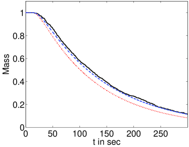
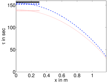
Figure 3: (Colour available online.) Comparing the experimental results (solid black line) to solutions of $\eqref{eq:classicalvjp}$ and $\eqref{eq:restingstate:p}$–$\eqref{eq:restingstate:r}$. Panel (a) shows the relative mass of the system over time. The dotted line (red) shows the numerical solution to equation $\eqref{eq:classicalvjp}$ with boundary conditions $\eqref{eq:classicalBC}$, the dashed line (blue) shows the numerical solution of the system of equations $\eqref{eq:restingstate:p}$–$\eqref{eq:restingstate:r}$ with boundary conditions $\eqref{eq:robotics:restingstate:BC}$. Panel (b) shows the mean exit time averaged over all velocity directions vs the x-coordinate along the arena edge. The adsorbing boundary is at x=1.183 m. The dotted line (red) shows the mean exit time computed using equation $\eqref{eq:meanExitTime}$ with boundary conditions $\eqref{eq:meanExitTimeBC}$, the dashed line (blue) shows the mean exit time computed using equation $\eqref{RevExitTimeProb}$ with boundary conditions $\eqref{tauboundaryconditionssim}$. In order to allow direct comparison with the experimental data, the shorter bold lines represent the average of theoretically derived exit times over the region $\Omega_{0}$, from which the robots were released in the experimental scenario. For both plots parameters and numerical methods are described in the text.

2.4 Comparison between theory and experiments: mean exit time problem

An alternative way to interpret the experimental data is to consider mean exit times. Throughout the experiments only $708$ of the $800$ ($=50\times 16$) robots left the arena before $t_{\mathrm{end}}=300\,\mathrm{sec}$. The average exit time of those $708$ robots was $121.92\,\mathrm{sec}$. In order to be able to compare experimental exit times with the mean exit time problems, it is necessary to estimate the mean exit time of all $800$ robots. Using the best exponential fit on the mass over time relation (cf. Figure 33), we can estimate the mean exit time of the remaining $92$ robots to be $424.69\,\mathrm{sec}$. The approximate mean exit time established in the experiments is therefore $156.74\,\mathrm{sec}$; this value is plotted as the solid (black) line in Figure 33. In order to be able to compare this value to analytic results, one has to reformulate the transport equation (1.1) into a mean exit time problem. Let us therefore define the mean exit time $\tau=\tau(\mathbf{x}_{0},\mathbf{v}_{0})$ of a robot that starts at position $\mathbf{x}_{0}\in\Omega$ with velocity $\mathbf{v}_{0}\in V$. This mean exit time satisfies the following equation

$$\mathbf{v}_{0}\cdot\nabla_{\mathbf{x}_{0}}\tau(\mathbf{x}_{0},\mathbf{v}_{0})-\lambda\tau(\mathbf{x}_{0},\mathbf{v}_{0})+\lambda\int_{V}{T(\mathbf{u}_{0},\mathbf{v}_{0})\tau(\mathbf{x}_{0},\mathbf{u}_{0})\,\mathrm{d}\mathbf{u}_{0}}=-1\,.$$ (2.5)

In Section 3, in which delays are modelled, a derivation is given for the mean exit time problem; setting the delay term to zero allows one to see how equation (2.5) is derived. This so-called “backwards problem” satisfies the following boundary conditions

$$\tau(\mathbf{x}_{0},\mathbf{v}_{0}) =0\,, \mathbf{x}_{0}\in\partial\Omega_{\mathcal{T}}\,,\mathbf{v}_{0}\cdot\mathbf{n}_{\mathcal{T}}>0\,,$$ (2.6)

$$\tau(\mathbf{x}_{0},\mathbf{v}_{0}) =\tau(\mathbf{x}_{0},\mathbf{v}_{0}^{\prime})\,, \mathbf{x}_{0}\in\partial\Omega_{\mathcal{R}}\,,$$

where $\mathbf{v}_{0}^{\prime}$ is again the reflected velocity with respect to $\mathbf{v}_{0}$ as defined in (2.3). Due to the arena shape, by taking the spatial average in the $y$-direction

$$\tau_{x}(x_{0},\mathbf{v}_{0})=\frac{1}{L_{y}}\int_{-L_{y}/2}^{L_{y}/2}\tau(x_{0},y_{0},\mathbf{v}_{0})\,\mathrm{d}y_{0},$$ (2.7)

one can further simplify the mean exit time problem. In the case where the turning kernel is given by equation (1.2), one can obtain a problem with two parameters $x_{0}$ and $\theta$, where $\theta\in(-\pi,\pi]$ is the angle defining the velocity $\mathbf{v}_{0}$ by $\mathbf{v}_{0}=s(\cos(\theta),\sin(\theta)).$ For $\tau_{x}=\tau_{x}(x_{0},\theta)$

$$s\cos(\theta)\frac{\partial\tau_{x}}{\partial x_{0}}-\lambda\tau_{x}+\frac{\lambda}{2\pi}\int_{-\pi}^{\pi}\tau_{x}(x_{0},\phi)\,\mathrm{d}\phi =-1\,,$$ (2.8)

$$\tau_{x}(0,\theta) =\tau_{x}(0,\pi-\theta)\,,$$

$$\tau_{x}(L_{x},\theta) =0\,, \;\;\theta\in\left[-\frac{\pi}{2},\frac{\pi}{2}\right].$$

When initial direction cannot be specified, the mean-exit time from a given $x$-position is given by

$$\frac{1}{2\pi}\int_{-\pi}^{\pi}\tau_{x}(x_{0},\theta)\,\mathrm{d}\theta,$$

where $\tau_{x}$ is the solution of (2.8). This is plotted as the dotted (red) line in Figure 33. The numerical solution was performed using an upwind-scheme in the $x$-direction with $\Delta x=1.1825\,\text{m}/200$ and an angular discretisation of $\Delta\theta=\pi/20$. Additionally, we take the spatial average of the mean-exit time from the initial region $\Omega_{0}$ and plot this as the bold dashed line in Figure 33. This line does not match well with the corresponding average mean-exit time found in the robot experiments. The numerical solution of equation (2.8) predicted a mean exit time of $137.49\,\mathrm{sec}$, meaning an underestimation of $19.25\,\text{sec}$ or $12.3\%$ compared to the experimental exit time of $156.74\,\mathrm{sec}$. In the following section we will extend the classical velocity jump theory to improve this match with the experimental data.

3 Modelling turning delays

In Section 2.2, we observed that collisions between robots does not play a major role in explaining the discrepancy between the transport equation (1.1) and the experimental data presented in Sections 2.3 and 2.4. As well as assuming independently moving particles, the transport equation (1.1) is also predicated on the assumption that the reorientation phase takes a negligible amount of time compared to the running phase. Since this assumption is not satisfied in our robot experiments, this section extends the original model through the inclusion of finite turning times.

3.1 Introduction of a resting state

Let us initially state two assumptions that apply to the robot experiment, but might not extend to velocity jump processes in biological systems, like the run-and-tumble motion of E. Coli (?), which has motivated the searching strategies implemented on robots:

(a) a new direction $\mathbf{v}^{\prime}\in V$ is chosen as soon as the particle enters the reorientation (“tumble”) phase;

(b) the time it takes for a particle to reorient (“tumble”) from velocity $\mathbf{v}\in V$ to $\mathbf{v}^{\prime}\in V$ is specified by the function $K(\mathbf{v}^{\prime},\mathbf{v}):V\times V\mapsto\mathbb{R}^{+}$.

Assumption (b) implies that the turning time is constant in time and equal for each particle and, in particular, does not depend on the particle’s history. For the robots studied in this paper, we can additionally assume that reorientation phase is equivalent to a directed rotation with a constant angular velocity $\omega\in\mathbb{R}^{+}$. Therefore, the turning time depends only on the angle between the current velocity $\mathbf{v}\in V$ and the new velocity $\mathbf{v}^{\prime}\in V$ and $K$ takes the form

$$K(\mathbf{v}^{\prime},\mathbf{v})=\frac{1}{\omega}\arccos\left(\frac{\mathbf{v}\cdot\mathbf{v}^{\prime}}{\left|\left|\mathbf{v}\right|\right|\;\left|\left|\mathbf{v}^{\prime}\right|\right|}\right).$$ (3.1)

We now extend the classical model (1.1) through the introduction of a resting state $r(t,\mathbf{x},\mathbf{v},\eta)$ that formally defines the number of particles currently “tumbling” (turning) towards their new chosen velocity $\mathbf{v}$ and remaining turning time $\eta$. The density $p(t,\mathbf{x},\mathbf{v})$ will now only denote the particles which are at time $t$ in the run phase. The update of the extended system is given through

$$\frac{\partial p}{\partial t}(t,\mathbf{x},\mathbf{v})+\mathbf{v}\cdot\nabla_{\mathbf{x}}p(t,\mathbf{x},\mathbf{v}) =-\lambda p(t,\mathbf{x},\mathbf{v})+r(t,\mathbf{x},\mathbf{v},0^{+})\,,$$ (3.2)

$$\frac{\partial r}{\partial t}(t,\mathbf{x},\mathbf{v},\eta)-\frac{\partial r}{\partial\eta}(t,\mathbf{x},\mathbf{v},\eta) =\lambda\int_{V}p(t,\mathbf{x},\mathbf{u})\,T(\mathbf{v},\mathbf{u})\,\delta(\eta-K(\mathbf{v},\mathbf{u}))\,\mathrm{d}\mathbf{u}\,.$$ (3.3)

In (3.2) we can see that running particles will enter a tumble phase with rate $\lambda$ and particles that have finished the tumble signified through $\eta=0$ will re-enter the run-phase. Equation (3.3) represents the linear relation between $t$ and $\eta$ and shows that particles enter the tumble phase depending on their newly chosen velocity direction. In order to guarantee conservation of mass throughout the system, we introduce the non-negativity condition for $\eta$ through

$$r(t,\mathbf{x},\mathbf{v},\eta)=0,\qquad\mbox{for}\qquad t>0,\quad\mathbf{x}\in\Omega,\quad\mathbf{v}\in V\quad\mbox{and}\quad\eta<0.$$

Additionally, the boundary conditions for the system (3.2)–(3.3) are given through

$$p(t,\mathbf{x},\mathbf{v}) =0\,, \mathbf{x}\in\partial\Omega_{\mathcal{T}}\,,\;\mathbf{v}\cdot\mathbf{n}_{\mathcal{T}}<0\,,\;$$ (3.4)

$$p(t,\mathbf{x},\mathbf{v}) =-r(t,\mathbf{x},\mathbf{v},0^{+})/(\mathbf{v}\cdot\mathbf{n}_{\mathcal{R}})\,, \mathbf{x}\in\partial\Omega_{\mathcal{R}}\,,\;\mathbf{v}\cdot\mathbf{n}_{\mathcal{R}}<0\,,$$

$$\frac{\partial r}{\partial t}(t,\mathbf{x},\mathbf{v},\eta)-\frac{\partial r}{\partial\eta}(t,\mathbf{x},\mathbf{v},\eta) =\delta(\eta-K(\mathbf{v},\mathbf{v}^{\prime}))\,(\mathbf{v^{\prime}}\cdot\mathbf{n}_{\mathcal{R}})\,p(t,\mathbf{x},\mathbf{v}^{\prime})\,, \mathbf{x}\in\partial\Omega_{\mathcal{R}}\,,\;\mathbf{v}\cdot\mathbf{n}_{\mathcal{R}}<0\,,$$

$$r(t,\mathbf{x},\mathbf{v},\eta) =0\,, \mathbf{x}\in\partial\Omega_{\mathcal{R}}\,,\;\mathbf{v}\cdot\mathbf{n}_{\mathcal{R}}>0\,,$$

where $\mathbf{v^{\prime}}$ is the reflected velocity of $\mathbf{v}$ given by (2.3). In order to show that the system (3.2)–(3.3) is actually consistent, we prove that mass in the system is conserved if no target is present.

Lemma 3.1

The total mass in system $\eqref{eq:restingstate:p}$–$\eqref{eq:restingstate:r}$ with the boundary conditions given in $\eqref{eq:robotics:restingstate:BC}$ in the case of reflective boundaries everywhere ($\partial\Omega_{\mathcal{R}}=\partial\Omega\,,\partial\Omega_{\mathcal{T}}=\emptyset$) given through

$$M(t)=\int_{\Omega}\int_{V}p(t,\mathbf{x},\mathbf{v})\,\mathrm{d}\mathbf{v}\,\mathrm{d}\mathbf{x}+\int_{\overline{\Omega}}\int_{V}\int_{0}^{\infty}r(t,\mathbf{x},\mathbf{v},\eta)\,\mathrm{d}\eta\,\mathrm{d}\mathbf{v}\,\mathrm{d}\mathbf{x}\,,$$

is conserved.

Proof.

We define for every point $\mathbf{x}\in\partial\Omega_{\mathcal{R}}$ the two subsets $V^{+}$ and $V^{-}$ of $V$ as follows

$$V^{+}(\mathbf{x})=\left\{\mathbf{v}\in V\ :\ \mathbf{v}\cdot\mathbf{n}_{\mathcal{R}}>0\right\}\,,\qquad V^{-}(\mathbf{x})=\left\{\mathbf{v}\in V\ :\ \mathbf{v}\cdot\mathbf{n}_{\mathcal{R}}<0\right\}\,.$$ (3.5)

Additionally, let us define

$$R(t,\mathbf{x},\mathbf{v})=\int_{0}^{\infty}r(t,\mathbf{x},\mathbf{v},\eta)\,\mathrm{d}\eta\,.$$

Integrating (3.3) with respect to $\eta\in[0,\infty)$, we obtain after reordering for $\mathbf{x}\notin\partial\Omega$:

$$\frac{\partial R}{\partial t}(t,\mathbf{x},\mathbf{v})=-r(t,\mathbf{x},\mathbf{v},0^{+})+\lambda\int_{V}p(t,\mathbf{x},\mathbf{u})T(\mathbf{v},\mathbf{u})\,\mathrm{d}\mathbf{u}\,.$$

Hence, for every point $\mathbf{x}\notin\partial\Omega$ we obtain

$$\frac{\partial}{\partial t}\left[p(t,\mathbf{x},\mathbf{v})+R(t,\mathbf{x},\mathbf{v})\right]=-\lambda p(t,\mathbf{x},\mathbf{v})+\lambda\int_{V}p(t,\mathbf{x},\mathbf{u})T(\mathbf{v},\mathbf{u})\,\mathrm{d}\mathbf{u}-\mathbf{v}\cdot\nabla_{\mathbf{x}}p(t,\mathbf{x},\mathbf{v})\,.$$

Integrating this with respect to $\mathbf{x}\in\Omega$ and $\mathbf{v}\in V$ gives

$$\int_{\Omega}\int_{V}\frac{\partial}{\partial t}\left[p(t,\mathbf{x},\mathbf{v})+R(t,\mathbf{x},\mathbf{v})\right]\,\mathrm{d}\mathbf{v}\,\mathrm{d}\mathbf{x}=-\int_{\Omega}\int_{V}\mathbf{v}\cdot\nabla_{\mathbf{x}}p(t,\mathbf{x},\mathbf{v})\,\mathrm{d}\mathbf{v}\,\mathrm{d}\mathbf{x}\,.$$ (3.6)

Using the divergence theorem, we can evaluate the integral on the right hand side to be

$$\int_{\Omega}\int_{V}\mathbf{v}\cdot\nabla_{x}p\,\mathrm{d}\mathbf{v}\,\mathrm{d}\mathbf{x} = \int_{\partial\Omega}\int_{V}(\mathbf{v}\cdot\mathbf{n}_{\mathcal{R}}(\mathbf{x}))\,p(t,\mathbf{x},\mathbf{v})\,\mathrm{d}\mathbf{v}\,\mathrm{d}\mathbf{x}$$

$$= \int_{\partial\Omega}\int_{V^{+}(\mathbf{x})}(\mathbf{v}\cdot\mathbf{n}_{\mathcal{R}})\,p(t,\mathbf{x},\mathbf{v})\,\mathrm{d}\mathbf{v}\,\mathrm{d}\mathbf{x}+\int_{\partial\Omega}\int_{V^{-}(\mathbf{x})}(\mathbf{v}\cdot\mathbf{n}_{\mathcal{R}})\,p(t,\mathbf{x},\mathbf{v})\,\mathrm{d}\mathbf{v}\,\mathrm{d}\mathbf{x}$$

$$= \int_{\partial\Omega}\int_{V^{+}(\mathbf{x})}(\mathbf{v}\cdot\mathbf{n}_{\mathcal{R}})\,p(t,\mathbf{x},\mathbf{v})\,\mathrm{d}\mathbf{v}\,\mathrm{d}\mathbf{x}-\int_{\partial\Omega}\int_{V^{-}(\mathbf{x})}r(t,\mathbf{x},\mathbf{v},0^{+})\,\mathrm{d}\mathbf{v}\,\mathrm{d}\mathbf{x}\,,$$

where we have used the second boundary condition in (3.4) in the last step. Additionally, for $\mathbf{x}\in\partial\Omega$ and $\mathbf{v}\in V^{-}(\mathbf{x})$, we obtain by integrating the third boundary condition in (3.4) with respect to $\eta\in[0,\infty)$

$$\frac{\partial R}{\partial t}(t,\mathbf{x},\mathbf{v})=-r(t,\mathbf{x},\mathbf{v},0^{+})+(\mathbf{v^{\prime}}\cdot\mathbf{n}_{\mathcal{R}})\,p(t,\mathbf{x},\mathbf{v^{\prime}})\,{.}$$

Integrating this with respect to $\mathbf{x}\in\partial\Omega$ and $\mathbf{v}\in V$ and using the last boundary condition in (3.4) we obtain

$$\int_{\partial\Omega}\int_{V}\frac{\partial R}{\partial t}\,\mathrm{d}\mathbf{v}\,\mathrm{d}\mathbf{x} = \int_{\partial\Omega}\int_{V^{-}(\mathbf{x})}\frac{\partial R}{\partial t}\,\mathrm{d}\mathbf{v}\,\mathrm{d}\mathbf{x}$$ (3.7)

$$= -\int_{\partial\Omega}\int_{V^{-}(\mathbf{x})}r(t,\mathbf{x},\mathbf{v},0^{+})\,\mathrm{d}\mathbf{v}\,\mathrm{d}\mathbf{x}+\int_{\partial\Omega}\int_{V^{-}(\mathbf{x})}(\mathbf{v^{\prime}}\cdot\mathbf{n}_{\mathcal{R}})\,p(t,\mathbf{x},\mathbf{v^{\prime}})\,\mathrm{d}\mathbf{v}\,\mathrm{d}\mathbf{x}$$

$$= -\int_{\partial\Omega}\int_{V^{-}(\mathbf{x})}r(t,\mathbf{x},\mathbf{v},0^{+})\,\mathrm{d}\mathbf{v}\,\mathrm{d}\mathbf{x}+\int_{\partial\Omega}\int_{V^{+}(\mathbf{x})}(\mathbf{v}\cdot\mathbf{n}_{\mathcal{R}})\,p(t,\mathbf{x},\mathbf{v})\,\mathrm{d}\mathbf{v}\,\mathrm{d}\mathbf{x}.$$

Summing up the results from (3.6) and (3.7), we obtain $\mbox{d}M/\mbox{d}t=0$ and hence the total mass $M(t)$ in the system is conserved. ∎

3.2 Transport equation with turning delays

We eliminate the resting state from system (3.2)–(3.3) and derive the generalization of the transport equation (1.1) to a transport equation with a suitably incorporated delay. This can be done by solving (3.3) for $r$ using the method of characteristics, which results in

$$r(t,\mathbf{x},\mathbf{v},0)=r(0,\mathbf{x},\mathbf{v},t)+\lambda\int_{V}T(\mathbf{v},\mathbf{u})\,p(t-K(\mathbf{v},\mathbf{u}),\mathbf{x},\mathbf{u})\,H(t-K(\mathbf{v},\mathbf{u}))\mathrm{d}\mathbf{u}\,,$$ (3.8)

where $H$ is the Heaviside step function. Let us assume that $K(\mathbf{v},\mathbf{u})$ is given by (3.1). Then $K(\mathbf{v},\mathbf{u})\leq\pi/\omega$. Considering times $t>\pi/\omega$, we have $r(0,\mathbf{x},\mathbf{v},t)=0$. We can now substitute (3.8) into (3.2) to obtain

$$\frac{\partial p}{\partial t}\,(t,\mathbf{x},\mathbf{v})+\mathbf{v}\cdot\nabla_{\mathbf{x}}\,p(t,\mathbf{x},\mathbf{v})=-\lambda p(t,\mathbf{x},\mathbf{v})+\lambda\int_{V}T(\mathbf{v},\mathbf{u})\,p(t-K(\mathbf{v},\mathbf{u}),\mathbf{x},\mathbf{u})\,\mathrm{d}\mathbf{u},$$ (3.9)

for $t>\pi/\omega$. Note that (3.9) only considers particles in the running phase and hence does not strictly conserve mass. The boundary conditions for transport equation (3.9) are

$$p(t,\mathbf{x},\mathbf{v}) =0\,, \mathbf{x}\in\partial\Omega_{\mathcal{T}}\,,\mathbf{v}\cdot\mathbf{n}_{\mathcal{T}}<0\,,$$ (3.10)

$$p(t,\mathbf{x},\mathbf{v}) =p(t-K(\mathbf{v},\mathbf{v^{\prime}}),\mathbf{x},\mathbf{v^{\prime}})\,, \mathbf{x}\in\partial\Omega_{\mathcal{R}}\,,\mathbf{v}\cdot\mathbf{n}_{\mathcal{R}}<0\,.$$

3.3 Equation for mean-exit time

Equation (3.9) can be rewritten as $\mathcal{M}p=0,$ where the operator $\mathcal{M}$ is given by

$$\mathcal{M}p=-\frac{\partial p}{\partial t}-\mathbf{v}\cdot\nabla_{\mathbf{x}}p-\lambda p+\lambda\int_{V}T(\mathbf{v},\mathbf{u})p(t-K(\mathbf{v},\mathbf{u}),\mathbf{x},\mathbf{u})\mathrm{d}\mathbf{u}.$$ (3.11)

For a forward problem specified by $\mathcal{M}p=0,$ coupled with initial and boundary conditions, the backward problem is given by the adjoint operator $\mathcal{M}^{*}q=0,$ with final condition and adjoint boundary conditions (?). The adjoint operator is given by:

$$\langle\mathcal{M}p,q\rangle=\langle p,\mathcal{M}^{*}q\rangle\quad\text{where}\quad\langle p,q\rangle=\int_{-\infty}^{\infty}\int_{\Omega}\int_{V}p(t,\mathbf{x},\mathbf{v})q(t,\mathbf{x},\mathbf{v})\,\mathrm{d}\mathbf{v}\,\mathrm{d}\mathbf{x}\,\mathrm{d}t.$$

Using integration by parts and the divergence theorem, we see

$$\langle\mathcal{M}p,q\rangle = \int_{-\infty}^{\infty}\int_{\Omega}\int_{V}\left(-\frac{\partial p}{\partial t}-\mathbf{v}\cdot\nabla_{\mathbf{x}}p-\lambda p+\lambda\int_{V}T(\mathbf{v},\mathbf{u})p(t-K(\mathbf{v},\mathbf{u}),\mathbf{x},\mathbf{u})\mathrm{d}\mathbf{u}\right)q\;\mathrm{d}\mathbf{v}\,\mathrm{d}\mathbf{x}\,\mathrm{d}t$$ (3.12)

$$= \int_{-\infty}^{\infty}\int_{\Omega}\int_{V}p\left(\frac{\partial q}{\partial t}+\mathbf{v}\cdot\nabla_{\mathbf{x}}q-\lambda q+\lambda\int_{V}T(\mathbf{u},\mathbf{v})q(t+K(\mathbf{u},\mathbf{v}),\mathbf{x},\mathbf{u})\mathrm{d}\mathbf{u}\right)\,\mathrm{d}\mathbf{v}\,\mathrm{d}\mathbf{x}\,\mathrm{d}t$$

$$+\int_{-\infty}^{\infty}\int_{V}\int_{\partial\Omega}p(t,\mathbf{x},\mathbf{v})q(t,\mathbf{x},\mathbf{v})[\mathbf{v}\cdot\mathbf{n}]\,\mathrm{d}S_{x}\,\mathrm{d}\mathbf{v}\,\mathrm{d}t$$

where we used the boundary conditions

$$\lim\limits_{t\to\infty}p(t,\mathbf{x},\mathbf{v})=\lim\limits_{t\to-\infty}q(t,\mathbf{x},\mathbf{v})\quad=0.$$ (3.13)

We will also assume the following boundary conditions

$$q(t,\mathbf{x},\mathbf{v}) =0\,, \mathbf{x}\in\partial\Omega_{\mathcal{T}}\,,\mathbf{v}\cdot\mathbf{n}_{\mathcal{T}}>0\,,$$ (3.14)

$$q(t,\mathbf{x},\mathbf{v}) =q(t+K(\mathbf{v}^{\prime},\mathbf{v}),\mathbf{x},\mathbf{v}^{\prime})\,, \mathbf{x}\in\partial\Omega_{\mathcal{R}}\,,\mathbf{v}\cdot\mathbf{n}_{\mathcal{R}}>0\,.$$

Then the last term in (3.12) is equal to zero as it is shown in Appendix B. Using (3.12)–(3.14) and the variable set $(t_{0},\mathbf{x}_{0},\mathbf{v}_{0})$ to indicate starting times and positions, we can write the backwards equation $\mathcal{M}^{*}q=0$ in the following form:

$$-\frac{\partial q}{\partial t_{0}}(t_{0},\mathbf{x}_{0},\mathbf{v}_{0})-\mathbf{v}_{0}\cdot\nabla_{\mathbf{x}_{0}}q(t_{0},\mathbf{x}_{0},\mathbf{v}_{0})=-\lambda q(t_{0},\mathbf{x}_{0},\mathbf{v}_{0})+\lambda\int_{V}{T(\mathbf{u}_{0},\mathbf{v}_{0})q(t_{0}+K(\mathbf{u}_{0},\mathbf{v}_{0}),\mathbf{x}_{0},\mathbf{u}_{0})\mathrm{d}\mathbf{u}_{0}}.$$ (3.15)

More precisely, we should write $q(t_{0},\mathbf{x}_{0},\mathbf{v}_{0})\equiv p(t,\mathbf{x},\mathbf{v}\,|\,t_{0},\mathbf{x}_{0},\mathbf{v}_{0})$, i.e. $q$ gives the probability that the particle is at the position $\mathbf{x}$ with velocity $\mathbf{v}$ at time $t$ given that its initial position and velocity at time $t_{0}$ were $\mathbf{x}_{0}$ and $\mathbf{v}_{0}$, respectively. Let $\rho\equiv\rho(t,\mathbf{x}_{0},\mathbf{v}_{0})$ be the probability that the particle is in $\Omega$ at time $t$ given that the initial position and velocity is given as $\mathbf{x}_{0}$ and $\mathbf{v}_{0}$, respectively. Then

$$\rho(t,\mathbf{x}_{0},\mathbf{v}_{0})=\int_{\Omega}\int_{V}p(t,\mathbf{x},\mathbf{v}\,|\,0,\mathbf{x}_{0},\mathbf{v}_{0})\,\mathrm{d}\mathbf{v}\,\mathrm{d}\mathbf{x}=\int_{\Omega}\int_{V}p(0,\mathbf{x},\mathbf{v}\,|\,-t,\mathbf{x}_{0},\mathbf{v}_{0})\,\mathrm{d}\mathbf{v}\,\mathrm{d}\mathbf{x}.$$

Substituting $t_{0}=-t$ into (3.15) and using the Taylor expansion, we obtain

$$\frac{\partial\rho}{\partial t}(t,\mathbf{x}_{0},\mathbf{v}_{0})-\mathbf{v}_{0}\cdot\nabla_{\mathbf{x}_{0}}\rho(t,\mathbf{x}_{0},\mathbf{v}_{0}) = -\lambda\rho(t,\mathbf{x}_{0},\mathbf{v}_{0})+\lambda\int_{V}T(\mathbf{u}_{0},\mathbf{v}_{0})\rho(t-K(\mathbf{u}_{0},\mathbf{v}_{0}),\mathbf{x}_{0},\mathbf{u}_{0})\,\mathrm{d}\mathbf{u}_{0}$$ (3.16)

$$= -\lambda\rho(t,\mathbf{x}_{0},\mathbf{v}_{0})+\lambda\int_{V}T(\mathbf{u}_{0},\mathbf{v}_{0})\,\rho(t,\mathbf{x}_{0},\mathbf{u}_{0})\,\mathrm{d}\mathbf{u}_{0}$$

$$-\lambda\int_{V}T(\mathbf{u}_{0},\mathbf{v}_{0})K(\mathbf{u}_{0},\mathbf{v}_{0})\frac{\partial\rho}{\partial t}(t,\mathbf{x}_{0},\mathbf{u}_{0})\,\mathrm{d}\mathbf{u}_{0}+\dots.$$

The probability of a single particle leaving $\Omega$ in time interval $[t,t+\mathrm{d}t)$ is $\rho(t,\mathbf{x}_{0},\mathbf{v}_{0})-\rho(t+dt,\mathbf{x}_{0},\mathbf{v}_{0})\approx-\partial\rho/\partial t(t,\mathbf{x}_{0},\mathbf{v}_{0})\,\mathrm{d}t$. Consequently, the expected exit time is given by

$$\tau(\mathbf{x}_{0},\mathbf{v}_{0})=-\int_{0}^{\infty}t\frac{\partial\rho}{\partial t}(t,\mathbf{x}_{0},\mathbf{v}_{0})\,\mathrm{d}t=\int_{0}^{\infty}\rho(t,\mathbf{x}_{0},\mathbf{v}_{0})\,\mathrm{d}t,$$

where we use the fact that $\rho(t,\mathbf{x}_{0},\mathbf{v}_{0})\to 0$ as $t\to\infty$. Integrating (3.16) over time, we obtain

$$\mathbf{v}_{0}\cdot\nabla_{\mathbf{x}_{0}}\tau(\mathbf{x}_{0},\mathbf{v}_{0})-\lambda\tau(\mathbf{x}_{0},\mathbf{v}_{0})+\lambda\int_{V}{T(\mathbf{u}_{0},\mathbf{v}_{0})\tau(\mathbf{x}_{0},\mathbf{u}_{0})\mathrm{d}\mathbf{u}_{0}}$$ (3.17)

$$\hskip 85.35826pt=-\left(1+\lambda\int_{V}T(\mathbf{u}_{0},\mathbf{v}_{0})K(\mathbf{u}_{0},\mathbf{v}_{0})\mathrm{d}\mathbf{u}_{0}\right)\,,$$

where we neglected the higher order terms. By Taylor-expanding the boundary terms from equation (3.10) and integrating in time, we obtain the following boundary conditions

$$\tau(\mathbf{x}_{0},\mathbf{v}_{0}) =0\,, \mathbf{x}_{0}\in\partial\Omega_{\mathcal{T}}\,,\;\mathbf{v}_{0}\cdot\mathbf{n}_{\mathcal{T}}>0\,,$$ (3.18)

$$\tau(\mathbf{x}_{0},\mathbf{v}_{0}^{\prime}) =\tau(\mathbf{x}_{0},\mathbf{v}_{0})+K(\mathbf{v}_{0}^{\prime},\mathbf{v}_{0})\,, \mathbf{x}_{0}\in\partial\Omega_{\mathcal{R}}\,,\;\mathbf{v}_{0}\cdot\mathbf{n}_{\mathcal{R}}>0\,,$$

where the reflected velocity $\mathbf{v}_{0}^{\prime}$ is given by (2.3), i.e. $\mathbf{v}_{0}^{\prime}=\mathbf{v}_{0}-2(\mathbf{v}_{0}\cdot\mathbf{n}_{\mathcal{R}})\mathbf{n}_{\mathcal{R}}$.

3.4 Comparison between the transport equation theory with delays and experimental results

Let us now compare the extended theory developed in Sections 3.1–3.3 to the experimental data using the same approach as in Sections 2.3 and 2.4. For the case of the arena given in Figure 1, we write $\Omega=(0,L_{x})\times(-L_{y}/2,L_{y}/2)$ and $\mathcal{T}=(L_{x},\infty)\times(-L_{y}/2,L_{y}/2)$ and we simplify equation (3.17) by integrating over the $y$-direction to obtain an average value for $\tau$ for our position along the $x$-axis. Let us define this average:

$$\tau_{x}(x_{0},\theta)=\frac{1}{L_{y}}\int_{-L_{y}/2}^{L_{y}/2}\tau(x_{0},y_{0},\mathbf{v}_{0})\mathrm{d}y_{0}.$$ (3.19)

By writing $\mathbf{v}_{0}=(v_{0}^{(x)},v_{0}^{(y)})$, integrating (3.17) and using (3.18), we obtain the following equation for $\tau_{x}$

$$v_{0}^{(x)}\frac{\partial\tau_{x}}{\partial x_{0}}-\frac{|v_{0}^{(y)}|\,K(\mathbf{v}_{0}^{\prime},\mathbf{v}_{0})}{L_{y}}-\lambda\tau_{x}+\lambda\int_{V}{T(\mathbf{u}_{0},\mathbf{v}_{0})\tau_{x}(x_{0},\mathbf{u}_{0})\mathrm{d}\mathbf{u}_{0}}$$ (3.20)

$$\hskip 85.35826pt=-\left(1+\lambda\int_{V}T(\mathbf{u}_{0},\mathbf{v}_{0})K(\mathbf{u}_{0},\mathbf{v}_{0})\mathrm{d}\mathbf{u}_{0}\right)\,.$$

In the case where $T$ is the unbiased, fixed-speed, 2-dimensional turning kernel given by (1.2) and using (3.1), we have $\mathbf{v}_{0}=(v_{0}^{(x)},v_{0}^{(y)})=s(\cos\theta,\sin\theta)$ and we can evaluate the second integral term in equation (3.20) explicitly to be

$$\int_{V}T(\mathbf{u}_{0},\mathbf{v}_{0})\,K(\mathbf{u}_{0},\mathbf{v}_{0})\,\mathrm{d}\mathbf{u}_{0}=\int_{\theta-\pi}^{\theta+\pi}\frac{1}{2\pi}\frac{1}{\omega}|\theta-\theta_{*}|\mathrm{d}\theta_{*}=\frac{\pi}{2\omega}.$$

Then (3.20) can be rewritten as follows

$$s\cos(\theta)\frac{\partial\tau_{x}}{\partial x_{0}}-\lambda\tau_{x}+\frac{\lambda}{2\pi}\int_{-\pi}^{\pi}\tau_{x}(x_{0},\phi)\mathrm{d}\phi=-\left(1+\frac{\pi\lambda}{2\omega}-\frac{2\,s\,A(\theta)}{L_{y}\,\omega}\right),$$ (3.21)

where $A(\theta)$ is defined by

$$A(\theta)=\left\{\begin{array}[]{ll}-(\pi+\theta)\sin(\theta),&\mbox{for}\quad\theta\in(-\pi,-\pi/2],\\ \theta\sin(\theta),&\mbox{for}\quad\theta\in[-\pi/2,\pi/2],\\ (\pi-\theta)\sin(\theta),&\mbox{for}\quad\theta\in[\pi/2,\pi].\\ \end{array}\right.$$

Interestingly, the contribution of free turning on the right-hand side of (3.21) is given as $\pi\lambda/(2\omega)$, which can be explained using a simple averaging argument, because every tumble takes an average time of $\pi/(2/omega)$.

The boundary conditions (3.18) simplify to

$$\tau_{x}(L_{x},\theta) =0\,, \theta\in(-\pi/2,\pi/2)\,,$$ (3.22)

$$\tau_{x}(0,\theta) =\tau_{x}(0,\pi-\theta)+\frac{\pi-2|\theta|}{\omega}\,, \theta\in(-\pi/2,\pi/2)\,.$$

The numerical solution of (3.21)–(3.22) can be further simplified by considering the symmetry in angle $\tau_{x}(x_{0},\theta)=\tau_{x}(x_{0},-\theta)$, i.e. it is sufficient to solve (3.21) where $(x_{0},\theta)$ are restricted to the domain $(0,L_{x})\times(0,\pi)$ with boundary conditions (3.22).

3.4.1 Comparison between theory and experiments: loss of mass over time

In this section, we show that the transport theory with delays better explains the experimental data with robots by considering the loss of mass over time, as we did in Section 2.3. In Figure 33, we plot the mass remaining in the system against time. The solid (black) line represents the experimental data, whilst the results of the classical theory are shown as dotted (red) line. The dashed (blue) line shows a numerical solution of system (3.2)–(3.3) that incorporates the finite reorientation time into the analysis. The numerical solution was achieved using a first order finite-volume method paired with an upwind scheme for (3.3). For (3.2) we used $\Delta x=1.183\,\text{m}/200$, $\Delta t=10^{-3}\,\text{sec}$ and $\Delta\theta=\pi/20$. For (3.3) we used the same $\Delta t=10^{-3}\,\text{sec}$ and a discretisation of $\Delta\eta=3.38\times 10^{-2}\,\text{sec}$ corresponding to the time it takes to turn from one velocity direction to the next. Figure 33 demonstrates that the inclusion of turning delays provides an improved match to the experimental data.

3.4.2 Comparison between theory and experiments: mean exit time problem

The mean exit time problem from Section 2.4 can also be better modelled by the transport equation theory with suitable incorporated delays as is demonstrated in Figure 33. The solid (black) line represents again the experimental data, whilst the classical results are shown as dotted (red) lines. The numerical solution of (3.21) with the boundary conditions (3.22) is shown as the dashed (blue) line. This numerical solution was obtained using the same method as in Section 2.4 and we again plot the average over the initial pen as a bold dashed line. The bold dashed line indicates a predicted mean exit time of $152.43\,\text{sec}$ compared to the experimental value $156.74\,\text{sec}$, an error of approximately $2.7\%$ or $4.31\,\text{sec}$. This represents a strong improvement to the discrepancy of $12.3\%$ seen for the model that neglected the turning events (dotted red line) and goes to show that turning times are indeed non-negligible and can be built into our model in a consistent manner.

4 Incorporation of a signal gradient

In this section, we are aiming to formulate velocity jump models that incorporate changing turning frequencies $\lambda$. In particular, we are interested in turning frequencies that depend on the current velocity of the robot as well as its position in the domain, i.e. $\lambda=\lambda(\mathbf{x},\mathbf{v})$. The general velocity jump model for this case can be formulated as (cf. (1.1))

$$\dfrac{\partial p}{\partial t}+\mathbf{v}\cdot\nabla_{\mathbf{x}}p=-\lambda(\mathbf{x},\mathbf{v})\,p+\int_{V}\lambda(\mathbf{x},\mathbf{u})\,T(\mathbf{v},\mathbf{u})\,p(t,\mathbf{x},\mathbf{u})\,\mathrm{d}\mathbf{u}\,,$$ (4.1)

with the boundary conditions given in (2.4). Similarly, we can formulate this system by incorporating the resting period (cf. (3.2)–(3.3))

$$\dfrac{\partial p}{\partial t} +\mathbf{v}\cdot\nabla_{\mathbf{x}}p =-\lambda(\mathbf{x},\mathbf{v})\,p(t,\mathbf{x},\mathbf{v})+r(t,\mathbf{x},\mathbf{v},0^{+})\,,$$ (4.2)

$$\dfrac{\partial r}{\partial t} -\dfrac{\partial r}{\partial\eta} =\int_{V}\lambda(\mathbf{x},\mathbf{u})\,p(t,\mathbf{x},\mathbf{u})\,T(\mathbf{v},\mathbf{u*})\,\delta(\eta-K(\mathbf{v},\mathbf{u}))\,\mathrm{d}\mathbf{u}\,,$$

with boundary conditions (3.4). The system (4.2) can again be formulated in the form of a delay differential equation (cf. (3.9))

$$\frac{\partial p}{\partial t}+\mathbf{v}\cdot\nabla_{\mathbf{x}}p=-\lambda(\mathbf{x},\mathbf{v})\,p+\int_{V}\lambda(\mathbf{x},\mathbf{u})\,T(\mathbf{v},\mathbf{u})\,p(t-K(\mathbf{v},\mathbf{u}),\mathbf{x},\mathbf{u})\,\mathrm{d}\mathbf{u}\,,$$ (4.3)

where boundary conditions take the form (3.10). Similarly to the derivation in Section 3.3, one can derive the backwards problem, with the mean first passage time equation taking the form (cf. (2.5))

$$\mathbf{v_{0}}\cdot\nabla_{\mathbf{x_{0}}}\tau-\lambda(\mathbf{x_{0}},\mathbf{v_{0}})\tau+\lambda(\mathbf{x_{0}},\mathbf{v_{0}})\int_{V}T(\mathbf{u},\mathbf{v_{0}})\,\tau(\mathbf{x_{0}},\mathbf{u})\,\mathrm{d}\mathbf{u}$$ (4.4)

$$\hskip 56.9055pt=-\left(1+\lambda(\mathbf{x_{0}},\mathbf{v_{0}})\int_{V}T(\mathbf{u},\mathbf{v_{0}})\,K(\mathbf{u},\mathbf{v_{0}})\,\mathrm{d}\mathbf{u}\right)\,,$$

with boundary conditions given in (2.6).

4.1 Experiments with a signal gradient

In order to compare these generalised velocity jump models to experimental results, we introduce an external signal into the robot experiments presented in Section 2.1. The signal is incorporated in the form of a colour gradient that can be measured by the light sensors on the bottom of the E-Puck robots. The colour gradient is layed out in such a way that it changes along the $x$-axis in Figure 1 with the darker end closer to the target area. The reaction of the robots to this colour gradient is implemented using the internal variable $z$ and a changing turning frequency $\lambda(z)$ that are updated according to

$$\frac{\mathrm{d}z}{\mathrm{d}t} =\frac{S-z}{t_{a}}\,,$$ (4.5)

$$\lambda =\lambda_{0}+\lambda_{0}\left(1-\alpha(S-z)\right)\,,$$

where $S\in[0,1]$ represents the measured signal with increasing values of $S$ indicating a darker colour in the gradient. The way the turning frequency is changed is motivated by models of bacterial chemotaxis ?.

According to results from ?, a macroscopic density formulation for the robotic system is given through the hyperbolic chemotaxis equation

$$\frac{1}{\lambda_{0}}\dfrac{\partial^{2}n}{\partial t^{2}}+\dfrac{\partial n}{\partial t}=\frac{s^{2}}{d\lambda_{0}}\Delta n-\nabla\cdot\left(n\frac{\alpha\lambda_{0}s^{2}t_{a}}{d\lambda_{0}(1+\lambda_{0}t_{a})}\nabla S\right)\,,$$ (4.6)

where $S:\Omega\mapsto\mathbb{R}$ indicates the colour gradient and $n(t,\mathbf{x})$ describes the concentration of robots in $\Omega$. Equation (4.6) can be approximated by the velocity jump process (4.1) with the form for the turning frequency given by

$$\lambda(\mathbf{x},\mathbf{v})=\lambda_{0}-\gamma\,\mathbf{v}\cdot\nabla S(\mathbf{x})\,,\qquad\gamma=\frac{\alpha t_{a}\lambda_{0}}{1+\lambda_{0}t_{a}}\,.$$ (4.7)

Because the gradient of the colour signal $S$ was chosen to be parallel to the $x$-axis in the experimental setting, we can again simplify the formulation of the exit time problem (4.4) by averaging along the $y$-axis. The resulting equation takes the form

$$s\cos\theta\,\dfrac{\partial\bar{\tau}}{\partial x}+\frac{2s\sin\theta}{L_{y}\omega}\min(\theta,\pi-\theta)-\lambda(x,\theta)\,\bar{\tau}+\frac{\lambda(x,\theta)}{\pi}\int_{0}^{\pi}\!\!\!\bar{\tau}(x,\theta_{*})\,\mathrm{d}\theta_{*}=-1-\lambda(x,\theta)\frac{\pi}{2\omega}\,,$$ (4.8)

where $\lambda(x,\theta)$ is given through

$$\lambda(x,\theta)=\lambda_{0}-\gamma\,s\cos\theta\,\dfrac{\partial S(x)}{\partial x}\,.$$ (4.9)

Because the colour changes linearly along the $x$-axis, we approximate the signal $S(x)$ by a linear function. The values at the end-points were taken directly from robot measurements and hence, $S(x)$ takes the form

$$S(x)=0.23+0.39\frac{x}{L_{x}}\,,\qquad\dfrac{\partial S}{\partial x}\approx 0.33\,\mathrm{m}^{-1}\,.$$ (4.10)

We will use this linear form of $S(x)$ for all comparisons between experimental data and the derived models.

4.2 Comparison between models and experimental results

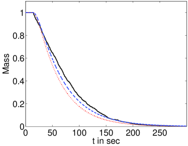
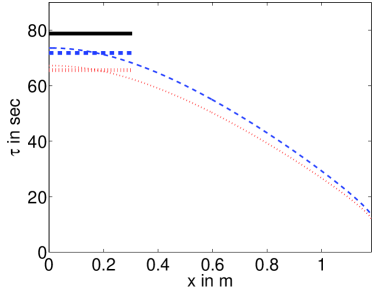
Figure 4: (Colour available online) Comparison between velocity jump process and experimental data for experiment including colour gradient. (a) Mean mass in system over time. Solid line (black): experimental data; dotted line (red): numerical solution of $\eqref{eq:gradient:VJP}$; dashed line (blue): numerical solution of $\eqref{eq:gradient:restingstate}$. Turning frequency $\lambda(\mathbf{x},\mathbf{v})$ as given in $\eqref{eq:robotics:signal:lambdaApp}$.
(b) Mean exit time averaged over all velocities. Solid line (black): experimental data; dotted line (red): numerical solution of $\eqref{eq:robotics:signal:MFPT:simple}$ for $\omega=\infty$; bold dotted line (red): average of dotted line over $\Omega_{0}$; dashed line (blue): numerical solution of $\eqref{eq:robotics:signal:MFPT:simple}$ for $\omega=4.65\,\mathrm{rad}\,\mathrm{sec}^{-1}$; bold dashed line (blue): average of dashed line over $\Omega_{0}$. Turning frequency $\lambda(x,\theta)$ as given in $\eqref{eq:robotics:signal:lambdaApp1D}$
For both plots parameters and numerical methods are given in the text.

We now want to compare the experimental data to the generalised velocity jump models presented in (4.1)–(4.9). The numerical solutions were achieved using the exact same methods and parameters as in Section 2.3 and the results can be seen in Figure 4. The parameter values used for the robots are $\lambda_{0}=0.25\,\mathrm{sec}^{-1}$, $\alpha=8$, $t_{a}=10\,\mathrm{sec}$ and $s=5.8\times 10^{-2}\,\text{m}/\text{sec}$. The experimental procedure was equivalent to the one presented in Section 2, i.e. we repeated the experiment 50 times with 16 robots, each time waiting until all of the 16 robots have left the arena.

In Figure 4(a) we plot the mass left in the system over time. The solid (black) line represents the percentage of robots still in the arena at that point in time. The dotted (red) line is a numerical solution of the velocity jump equation (4.1) with the corresponding boundary conditions (2.4). The dashed (blue) line is a numerical solution of the velocity jump system with resting state given in (4.2) and boundary conditions as in (3.4).

In Figure 4(b) we plot the mean exit time in dependence of position along the $x$-axis. The horizontal solid (black) line again indicates the experimentally measured exit time of $78.77\,\mathrm{sec}$. The dotted (red) line shows a numerical solution of (4.8) with instant turning, i.e. $\omega=\infty$. The dashed (blue) line shows a numerical solution of (4.8) with $\omega=4.65\,\mathrm{rad}\,\mathrm{sec}^{-1}$. For both of these solutions the boundary conditions are given in (2.6). The bold horizontal lines again indicate the average over the initial pen $\Omega_{0}$.

In both plots in Figure 4, we see that the models including finite turning delays (represented through the dashed (blue) lines) give an improved match compared to the models without this delay. The numerically estimated exit time for the model with instant turning ($\omega=\infty$) is $65.59\,\mathrm{sec}$ (error of $16.7\%$ compared to experimental data); with finite turning times it is $71.76\,\mathrm{sec}$ (error of $8.9\%$). The remaining difference between the models and the experimental data can be explained by noisy measurement of the signal $S(\mathbf{x})$ as well as the fact that we used linear approximation (4.10) averaged over all robots to obtain the numerical results. We can conclude from this brief study of robot experiments including a colour gradient signal that this signal indeed improves the target finding capacity of the robots and that the models developed in Section 3 can be generalised to incorporate turning frequencies that change according to external signals.

5 Discussion

In this paper, we have studied an implementation of a run-and-tumble searching strategy in a robotic system. The algorithm implemented by the robots is motivated by a biological system – behaviour of the flagellated bacterium E. coli. Bio-inspired algorithms are relatively common in swarm robotics. Algorithms based on behaviour of social insects have been implemented previously in the literature, see for example ??? and ?. One of the challenges of bio-inspired algorithms is that robots do not have the same sensors as animals. For example, E. coli bias their movement according to extracellular chemical systems. In biological models, chemical signals often evolve according to the solution of reaction-diffusion partial differential equations (??). Therefore, an implementation of the full run-and-tumble chemotactic model in the robotic system requires either special sensors for detecting chemical signals, e.g. robots for odour detecting (?), or replacing chemical signals by suitable caricatures of them, e.g. using glowing floor for E-Puck robots (?).

The main goal of this paper is to study how the mathematical theory developed for E. coli applies to the robotic system based on E-Pucks. Thus we do not focus on technological challenges connected with sensing changing chemical signals or their analogues (??), we do, however, incorporate a constant signal in order to show that the developed theory works for unbiased as well as biased velocity jump processes. If the collisions between particles (robots or bacteria) and reorientation times can be neglected, then this velocity jump process is described by the transport equation (1.1) or (4.1) (in the biased case) and the long time behaviour is given by a drift-diffusion equation (?). In Section 2.2 we show that collisions between robots are negligible in our experimental set up. However, we still observe quantitative differences between the results based on the transport equation (1.1) and robotic experiments.

In Section 3 we identify turning delays as the main mechanism contributing to differences between the mathematical theory developed for E. coli and the results of experiments with E-Pucks. We introduce the resting state in equations (3.2)–(3.3) and then derive the transport equation with delay (3.9). Our delay term is different from models of tumbling of E. coli, because the underlying physical process is different. Tumbling times of E. coli are exponentially distributed, i.e. they can be explicitly included in mathematical models by using transport equations which take into account probabilistic changes to and from the resting (tumbling) state (?). In the case of robots, the turning time depends linearly on the turning angle. The selection of new direction is effectively instant and the main contributing factor to turning delays is the finite turning speed of robots. In Section 4 we apply the developed theory to an experiment incorporating an external signal and show that similar transport equations can be developed for this situation.

We have studied a relatively simple searching algorithm motivated by E. Coli behaviour, but the transport equations and velocity jump processes naturally appear in modelling of other biological systems, such as modelling chemotaxis of amoeboid cells (?) or swarming behaviour as seen in various fish, birds and insects (??). We conclude that the same delay terms as in (3.9) would be applicable whenever we implement these models in E-Pucks. From a mathematical point of view, it is also interesting to consider coupling of (3.9) with changing extracellular signals, because signal transduction also has its own delay which can be modelled using velocity jump models with internal dynamics (???). Considering higher densities of robots, the transport equation formalism needs to be further adapted to incorporate the effects of robot-robot interactions. We have recently investigated this problem and reported our results in ?.

Appendix Appendix A Robot specifications

A photo of a collection of E-Puck robots and the arena are given in Figure 5. Full details of the E-Puck specifications are:

• Diameter: 75 mm. Height: 50 mm. Weight: 200g.

• Speed throughout experiments: $5.8\times 10^{-2}\,\text{m}\,\text{sec}^{-1}$, (max speed: $0.13\,\text{m}\,\text{sec}^{-1}$).

• Turning speed throughout experiments: $4.65\,\text{rad}\,\text{sec}^{-1}$.

• Processor: dsPIC 30 CPU @ 30 MHz (15 MIPS), (PIC Microcontroller.)

• RAM: 8 KB. Memory: 144 KB Flash.

• Autonomy: 2 hours moving. 2 step motors. 3D accelerometers.

• 8 infrared proximity and light, (TCRT1000)

• Colour camera, 640x480,

• 8 LEDs on outer ring, one body LED and one front LED,

• 3 microphones, forming a triangle allowing the determination of the direction of audio cues.

• 1 loudspeaker.

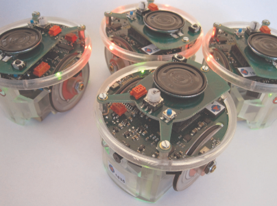
  (a)            (b)

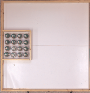
Figure 5: (a) Collection of E-Puck robots. (b) Photo showing the arena built for the experiments, removable pen and edges made from cut down medium density fibre.

Appendix Appendix B Derivation of adjoint boundary condition (3.14)

Using (2.1) and (3.5), the last term in (3.12) can be rewritten as follows

$$\int_{-\infty}^{\infty}\int_{V}\int_{\partial\Omega}p(t,\mathbf{x},\mathbf{v})q(t,\mathbf{x},\mathbf{v})[\mathbf{v}\cdot\mathbf{n}]\,\mathrm{d}S_{x}\,\mathrm{d}\mathbf{v}\,\mathrm{d}t$$

$$\hskip 28.45274pt=\int_{-\infty}^{\infty}\int_{\partial\Omega_{\mathcal{R}}\cup\partial\Omega_{\mathcal{T}}}\int_{V^{+}}\big{\{}p(t,\mathbf{x},\mathbf{v})q(t,\mathbf{x},\mathbf{v})-p(t,\mathbf{x},\mathbf{v}^{\prime})q(t,\mathbf{x},\mathbf{v}^{\prime})\big{\}}[\mathbf{v}\cdot\mathbf{n}]\,\mathrm{d}\mathbf{v}\,\mathrm{d}S_{x}\,\mathrm{d}t\,,$$

where $\mathbf{v}^{\prime}$ is given by (2.3). Separating the above integral into the cases of $\partial\Omega_{\mathcal{R}}$ and $\partial\Omega_{\mathcal{T}}$, and using the boundary condition (3.10), we have

$$\int_{-\infty}^{\infty}\int_{V}\int_{\partial\Omega}p(t,\mathbf{x},\mathbf{v})q(t,\mathbf{x},\mathbf{v})[\mathbf{v}\cdot\mathbf{n}]\,\mathrm{d}S_{x}\,\mathrm{d}\mathbf{v}\,\mathrm{d}t$$

$$\hskip 28.45274pt=\int_{-\infty}^{\infty}\int_{\partial\Omega_{\mathcal{R}}}\int_{V^{+}}\left\{p(t,\mathbf{x},\mathbf{v})q(t,\mathbf{x},\mathbf{v})-p\left(t-K(\mathbf{v}^{\prime},\mathbf{v}),\mathbf{x},\mathbf{v}\right)q(t,\mathbf{x},\mathbf{v}^{\prime})\right\}[\mathbf{v}\cdot\mathbf{n}]\,\mathrm{d}\mathbf{v}\,\mathrm{d}S_{x}\,\mathrm{d}t$$

$$\hskip 39.83368pt-\int_{-\infty}^{\infty}\int_{\partial\Omega_{\mathcal{T}}}\int_{V^{+}}\left\{p\left(t,\mathbf{x},\mathbf{v}^{\prime}\right)q\left(t,\mathbf{x},\mathbf{v}^{\prime}\right)\right\}[\mathbf{v}\cdot\mathbf{n}]\,\mathrm{d}\mathbf{v}\,\mathrm{d}S_{x}\,\mathrm{d}t\,.$$

We shift the time variable in the first term on the right hand side to deduce

$$\int_{-\infty}^{\infty}\int_{V}\int_{\partial\Omega}p(t,\mathbf{x},\mathbf{v})q(t,\mathbf{x},\mathbf{v})[\mathbf{v}\cdot\mathbf{n}]\,\mathrm{d}S_{x}\,\mathrm{d}\mathbf{v}\,\mathrm{d}t$$

$$\hskip 28.45274pt=\int_{-\infty}^{\infty}\int_{\partial\Omega_{\mathcal{R}}}\int_{V^{+}}p(t,\mathbf{x},\mathbf{v})\left\{q(t,\mathbf{x},\mathbf{v})-q\left(t+K(\mathbf{v}^{\prime},\mathbf{v}),\mathbf{x},\mathbf{v}^{\prime}\right)\right\}[\mathbf{v}\cdot\mathbf{n}]\,\mathrm{d}\mathbf{v}\,\mathrm{d}S_{x}\,\mathrm{d}t$$

$$\hskip 39.83368pt-\int_{-\infty}^{\infty}\int_{\partial\Omega_{\mathcal{T}}}\int_{V^{+}}\left\{p\left(t,\mathbf{x},\mathbf{v}^{\prime}\right)q\left(t,\mathbf{x},\mathbf{v}^{\prime}\right)\right\}[\mathbf{v}\cdot\mathbf{n}]\,\mathrm{d}\mathbf{v}\,\mathrm{d}S_{x}\,\mathrm{d}t\,.$$

The first term on the right hand side is zero because $q(t+K(\mathbf{v}^{\prime},\mathbf{v}),\mathbf{x},\mathbf{v}^{\prime})=q(t,\mathbf{x},\mathbf{v})$ in (3.14). The second term vanishes when $q(t,\mathbf{x},\mathbf{v}^{\prime})=0$. Thus we conclude that the last term in (3.12) is equal to zero when $q$ satisfies the boundary conditions (3.14).