Quantum magnetism of ultracold atoms with a dynamical pseudospin degree of freedom

Abstract

We consider bosons in a Hubbard lattice with an SU($\cal N$) pseudospin degree of freedom which is made dynamical via a coherent transfer term. It is shown that, in the basis which diagonalizes the pseudospin coupling, a generic hopping process affects the spin state, similar to a spin-orbit coupling. This results, for the system in the Mott phase, in a ferromagnetic phase with variable quantization axis. In extreme cases, it can even give rise to antiferromagnetic order.

I Introduction

Ultracold atoms in optical lattices are almost ideal realizations of different Hubbard models. In certain limits, these models can be directly mapped on spin models which are the key for understanding quantum magnetism and related phenonema like antiferromagnetism or spin liquids Auerbach (1994); M. Lewenstein et al. (2012). A particularly rich behavior can be explored by filling the lattice with multi-component atoms in Mott states. The most prominent example, recently realized experimentally Greif et al. (2013), is the two-component Fermi gas. In the Mott phase with one atom per site, such system is perfectly described by the antiferromagnetic Heisenberg model Hofstetter et al. (2002). The use of fermionic alkali earth atoms in optical lattices has been proposed to study SU($\cal N$) magnetism for $\cal N$ much larger than 2 Gorshkov et al. (2010). Attention has also been put on bosonic two-component systems Altman et al. (2003), or bosonic spinor gases with $F=1$ Demler and Zhou (2002); Imambekov et al. (2003); Yip (2003); García-Ripoll et al. (2004) or $F=2$ Barnett et al. (2006).

One can further enrich such systems by a laser coupling of the atomic states. If spatially dependent, such a coupling connects internal with external degrees of freedom, and can thus be interpreted a non-Abelian artificial gauge field Dalibard et al. (2011). The Mott transition in a bosonic Hubbard model is dramatically modified by the presence of such a field Graß et al. (2011), and deep in the Mott phase the gauge field supports phases with exotic magnetic ordering Cole et al. (2012); Radić et al. (2012). Recently, it has been pointed out in Ref. Boada et al. (2012) that the internal degrees of freedom can also be used for simulating an “extradimension”, once the internal states are properly coupled to provide the hopping between the synthetic sites given by the atomic species.

In this paper, we study the case of a spatially homogeneous coupling of the atomic states, and analyze the Mott phases in an $\cal N$-component Bose-Hubbard model in the presence of coherent transfer between the internal states. In the extradimension picture of Ref. Boada et al. (2012), the internal degree of freedom becomes equivalent to a compactified spatial dimension. Assuming SU($\cal N$) symmetry, we show in Sec. II that, in the appropriate spin basis, the internal hopping acts as an external magnetic field. It is responsible for a linear Zeeman shift lifting the degeneracy between the internal states.

In Sec. III, we then focus on a scenario where SU($\cal N$) symmetry is broken, and consider systems with state-dependent hopping strengths, as in the case of spin-dependent lattices Liu et al. (2004). Quite generally, a hopping process will then also change a particle’s internal state in the eigenbasis of the coupling. As it has been proposed in Ref. Eckardt et al. (2010), by shaking the optical lattice it is even possible to reverse the sign of the hopping term. In combination with spin-dependent lattices, this technique becomes species-selective and allows for generating non-Abelian hopping terms Hauke et al. (2012). This includes the case of a hopping of the form $J\sigma_{z}$, with $\sigma_{z}$ a Pauli matrix in SU(2), and similar expressions for higher spin. We extend our study to such extreme deviations from the SU($\cal N$)-symmetric hopping, and carefully analyze the SU(2) scenario. We find that deviations from an SU($\cal N$)-symmetric hopping rotate the quantization axis of a ferromagnetic phase. The full reversal of one hopping strength gives rise to a spin-rotated superexchange interaction, which favors unmagnetized states. This allows for a transition to an antiferromagnetic or checkerboard phase, that is to say, the superposition of pseudo-spin states becomes position-dependent following a crystal structure. In the extradimension picture, in which the different pseudo-spin states become different sites, such structures become density structures.

Afterwards, in Sec. IV, we consider an SU($\cal N$) symmetry breaking in the interaction term. In particular, we assume the interspecies density-density interaction as a free parameter. The resulting model interpolates between an SU(${\cal N}$) Bose-Hubbard system in $d$ dimensions, and ${\cal N}$ copies of a Bose-Hubbard system in $d+1$ space dimensions, respectively. Such model displays a rich Mott regime which can be perturbed to give rise to different phases. In particular, we focus on the parameter region that admits as degenerate ground states Mott configurations with the number $n$ of particles per site being non-commensurable with the number of species ${\cal N}$. We study in detail the paradigmatic example of $n=q{\cal N}+1$, with $q$ integer, i.e. one spin component is occupied by $q+1$ particles per site, while the other components are occupied with $q$ ones. At the perturbative level, the hopping terms induce a novel Potts-like effective Hamiltonian that displays different quantum phases. The different phases can be detected in time-of-flight absorption pictures by applying real magnetic fields for a Stern-Gerlach-type measurement.

II System

We consider an $\cal N$-component Bose gas in a hypercubic optical lattice in $d$ dimensions. The physics is well described by a Bose-Hubbard (BH) Hamiltonian $H=H_{I}+H_{J}+H_{0}$, where $H_{0}$ is the local interaction term, $H_{J}$ the hopping term, and $H_{I}$ the coherent transfer (internal hopping) between the pseudospin components. For $H_{0}$ we write:

$$H_{0}=\sum_{i,\sigma}\left[\left(\frac{U}{2}\hat{n}_{i}^{\sigma}(\hat{n}_{i}^{\sigma}-1)-\mu\hat{n}_{i}^{\sigma}\right)+\frac{U_{d}}{2}\sum_{\sigma^{\prime}}\hat{n}_{i}^{\sigma}\hat{n}_{i}^{\sigma^{\prime}}\right],$$ (1)

with $\hat{n}_{i}^{\sigma}\equiv\hat{a}_{i}^{(\sigma)\dagger}\hat{a}_{i}^{(\sigma)}.$ The operator $\hat{a}_{i}^{(\sigma)\dagger}$ creates a particle on site $i$ in the pseudospin state labeled by $\sigma$. The parameters $U$ and $U_{d}$ fix the (possibly) spin-dependent interaction strength. Many atoms, amongst them ⁸⁷Rb, possess hyperfine states with almost the same $s$-wave scattering lengths, thus, they are approximately described by $H_{0}$, with $U\approx U_{d}$. is $U=U_{d}$. The chemical potential $\mu$ allows to fix the total number of particles per site.

Note that $H_{0}$ is quadratic in $\hat{n}^{\sigma}$, $H_{0}=\frac{1}{2}{\bf v}^{\rm t}\cdot M\cdot{\bf v}-{\bf w}\cdot{\bf v}$, where ${\bf v}^{\rm t}\equiv(\hat{n}^{1},\dots,\hat{n}^{\cal N})$, and can be easily minimized by diagonalizing $M_{\sigma\rho}\equiv u+(1-u)\delta_{\sigma\rho}$, with $u\equiv\frac{U_{d}}{U}$, $\sigma,\rho=1,\dots\cal N$, and ${\rm w}_{\sigma}=\frac{\mu-U/2}{U}$. The content and the dimension of the minimal energy subspace depend strongly on the values of $u$ and of the chemical potential $\mu$, see Appendix A for details.

For the external hopping, $H_{J}$, we take into account a possibly spin-dependent nearest-neighbor tunneling:

$$H_{J} =-\sum_{\sigma}J^{(\sigma)}\sum_{\langle ij\rangle}\hat{a}_{i}^{(\sigma)\dagger}\hat{a}_{j}^{(\sigma)}.$$ (2)

Here, $J^{(\sigma)}$ is the pseudospin-dependent tunneling strength.

A coherent transfer term $H_{I}$ locally replaces a $\sigma$ particle by a $\sigma\pm 1$ particle. For convenience, we choose periodic boundaries for this “internal” hopping, that is, we shall take the value of $\sigma$ modulo ${\cal N}$:

$$H_{I}=-I\sum_{i,\sigma}\left(\hat{a}_{i}^{(\sigma)\dagger}\hat{a}_{i}^{({\rm mod}[\sigma+1,{\cal N}])}e^{i\phi}+\mathrm{H.c.}\right),$$ (3)

Experimentally, this term can be implemented by a resonant radio frequency in the linear Zeeman splitting regime of the hyperfine states (for open boundaries conditions) or by Raman lasers (for periodic boundary conditions, in the quadratic Zeeman splitting regime for ${\cal N}>3$) shining onto the atoms, see Celi et al. (2014). The laser intensity defines the coupling strength $I>0$, and the photons may also imprint a phase angle $\phi$. Note that for ${\cal N}\phi\neq 2\pi{\cal Z}$, under a full loop in the species space the state acquires a non-trivial phase. In the extradimension picture, this is equivalent to flux compactification of the synthetic $d+1$ dimension on a circle, with a magnetic flux piercing it. The Hamiltonian $H_{I}$ can be expressed as a circulant matrix $C$, such that $H_{I}=IC$ with

$$C=-\begin{bmatrix}c_{1}&c_{2}&\dots&c_{{\cal N}-1}&c_{{\cal N}}\\ c_{{\cal N}}&c_{1}&c_{2}&&c_{{\cal N}-1}\\ \vdots&c_{{\cal N}}&c_{1}&\ddots&\vdots\\ c_{3}&&\ddots&\ddots&c_{2}\\ c_{2}&c_{4}&\dots&c_{{\cal N}}&c_{1}\\ \end{bmatrix},$$ (4)

with $c_{2}=e^{i\phi}$ and $c_{{\cal N}}=e^{-i\phi}$, while $c_{i}=0$ for $i=1$ and $3\leq i\leq{\cal N}-1$. Eigenvalues $\lambda_{\alpha}$ and the corresponding eigenvectors ${\bm{v}}_{\alpha}$ of this matrix are given in terms of exponential terms $\omega_{\alpha}\equiv\exp[(2\pi i/N)\alpha]$:

$${\bm{v}}_{\alpha}=\frac{1}{\sqrt{{\cal N}}}(\omega_{\alpha}^{0},\omega_{\alpha}^{1},\cdots,\omega_{\alpha}^{{\cal N}-1})^{T},$$ (5)

and

$$\lambda_{\alpha}=2\cos[\phi+(2\pi i/{\cal N})\alpha].$$ (6)

We note that the eigenvectors are independent from the phase shift $\phi$. On the other hand, the eigenvalues can be tuned by this parameter. In particular, we can make any ${\bm{v}}_{\alpha}$ the ground state of $H_{I}$. Alternatively, any pair ${\bm{v}}_{\alpha}$ and ${\bm{v}}_{{\rm mod}[\alpha+1,{\cal N}]}$ can be made a two-fold degenerate ground state. With the choice of $H_{I}$ as in Eq. (3), higher degeneracies are not possible, but it is worth to notice that by turning on next-to-nearest neighbor coupling of the species as well, fourfold degeneracy of the eigenvalues can be achieved. Such coupling can be realistically laser induced as the ones described above.

It is convenient to introduce a matrix $V=[{\bm{v}}_{1},\cdots,{\bm{v}}_{\cal N}]$ which transforms from the original pseudospin basis into the basis of eigenstates of $H_{I}$. Starting by the Fock operators in the old basis organized as an SU$({\cal N})$-vector operator ${\bm{a}}_{i}\equiv(\hat{a}_{i}^{(1)},\cdots,\hat{a}_{i}^{({\cal N})})^{T}$, which in every component annihilates a particle in the original basis, we obtain the corresponding Fock operators in the novel basis as ${\bm{A}}_{i}\equiv V{\bm{a}}_{i}\equiv(\hat{A}_{i}^{(1)},\cdots,\hat{A}_{i}^{({\cal N})})$, which componentwise annihilates a particle in the state ${\bm{v}}_{\alpha}$.

Let us first discuss the case where $H_{0}$ and $H_{J}$ are SU($\cal N$) symmetric, that is $J^{(\sigma)}=J$ and $U=U_{d}$. We can write the full Hamiltonian as

$$H= \sum_{i}\left(\frac{U}{2}\hat{N}_{i}(\hat{N}_{i}-1)-\mu\hat{N}_{i}\right)-J\sum_{\langle ij\rangle}{\bm{A}}_{i}^{\dagger}{\bm{A}}_{j}+$$

$$I\sum_{i,\alpha}\lambda_{\alpha}\hat{A}_{i}^{(\alpha)\dagger}A_{i}^{(\alpha)}.$$ (7)

We can associate the eigenvalues $\lambda_{\alpha}$ with a magnetic quantum number. The internal coupling $I$ then can be interpreted a Zeeman shift $I\lambda_{\alpha}$ experienced by the state $\alpha$. This analogy to the atomic finestructure is best drawn if the levels are equally spaced. For $H_{I}$ of the form (3), this condition can be realized by choosing the proper $\phi$ for ${\cal N}\leq 4$, but not for higher values of ${\cal N}$ (at least if we limit to nearest neighbor species coupling in $H_{I}$). In fact, in order to get an equally spaced spectrum the coupling $I$ should depend on $\sigma$. For real nearest neighbor hoppings, $H_{I}$ has to be taken proportional to the normalization of the raising operator $F_{+}=F_{x}+iF_{y}$ for fixed total angular momentum $F$ such that $I^{(\sigma)}=I\sqrt{({\cal N}-\sigma)\sigma}$ for ${\cal N}=2F+1$. Note that this is exactly the coupling induced by Raman lasers in the far-detuned regime, as shown in Goldman et al. (2013); Dudarev et al. (2004); Juzeliūnas and Spielman (2012); Hügel and Paredes (2013) and considered in Celi et al. (2014) to simulate synthetic edge states with a synthetic dimension.

It is obvious that the last term of Eq. (II) breaks the SU($\cal N$) symmetry. The ground state properties of the system then become independent from the existence of the “internal dimension”, that is, the extradimension vanishes. For special choices of $\phi$, however, a two-fold degeneracy may remain.

III Magnetic orderings in systems with SU($\cal N$) symmetry-breaking hopping terms

Deviations from SU($\cal N$) symmetry in the hopping naturally occur if the atomic states possess different polarizabilities. One may also generate extreme deviations artificially using techniques for manipulating the hopping term. Such techniques have been developed in the context of simulating gauge fields. As discussed in Ref. Hauke et al. (2012) for SU(2) systems, it is, for instance, possible to reverse the hopping in one component via shaking.

How deviations from SU($\cal N$) symmetry enrich the physics of the system becomes transparent when we transform $H_{J}$ into the ${\bm{v}}_{\alpha}$ basis which diagonalizes $H_{I}$. Defining a vector ${\bm{J}}\equiv(J_{1},\cdots,J_{N})^{T}$ with the different hopping parameters in its components, we construct a matrix

$$Q_{kl}\equiv\left\{\begin{array}[]{cl}{\bm{J}}\cdot{\bm{v}}_{k-l},&\mbox{if }k\geq l\\ {\bm{J}}\cdot{\bm{v}}_{N+k-l},&\mbox{else}\end{array}\right.$$ (10)

With this matrix, we can write the hopping term as

$$H_{J}=\sum_{\langle ij\rangle}{\bm{A}}_{i}^{\dagger}\cdot Q\cdot{\bm{A}}_{j}.$$ (11)

Thus, in the new basis, hopping processes in $H_{J}$ in general not only change the external position of the particle, but also its internal state. The Hamiltonian is thus equivalent to one coupled to some constant non-Abelian gauge field. Hopping processes $\alpha\rightarrow\alpha$, that is, those which do not change the internal state have a hopping strength $j_{N}\equiv{\bm{J}}\cdot{\bm{v}}_{N}=\frac{1}{N}\sum_{\sigma=1}^{N}J^{(\sigma)}$. Hopping processes $\alpha\rightarrow{\rm mod}[\alpha+k,N]$ have a hopping strength $j_{k}\equiv{\bm{J}}\cdot{\bm{v}}_{k}$. Hence, the hopping term is generically complex. Note that $j_{k}=j_{N-k}^{*}$, that is, they can not independently be chosen.

Setting $J^{(\sigma)}\ll U$, we are deep in the Mott phase, and the Hamiltonian is solved by a Fock state of $n$ atoms per site. The number $n$ is tuned by the chemical potential $\mu$, which in the following is chosen such that $n=1$.

In the remainder of this section, we will first discuss in detail the consequences of such symmetry-breaking hopping on the Mott phase of a two-component Bose system. Afterwards, we will also take a brief look on systems with ${\cal N}>2$ components.

III.1 Two-component system

In SU(2), the hopping matrix $H_{I}$ is explicitly diagonalized by the operators

$$\hat{A}_{i} \equiv\frac{1}{\sqrt{2}}\left(\hat{a}_{i}^{(a)}+e^{i\phi}\hat{a}_{i}^{(b)}\right),$$ (12)

$$\hat{B}_{i} \equiv\frac{1}{\sqrt{2}}\left(\hat{a}_{i}^{(a)}-e^{i\phi}\hat{a}_{i}^{(b)}\right).$$ (13)

In this basis, it reads

$$H_{I}=-I\sum_{i}\left(\hat{A}_{i}^{\dagger}\hat{A}_{i}-\hat{B}_{i}^{\dagger}\hat{B}_{i}\right).$$ (14)

This expression shows that the phase $\phi$ is completely absorbed in the operators $\hat{A}$ and $\hat{B}$. The ground state now is uniquely given by the state $\left|A\right\rangle$.

Transforming $H_{J}$ into the $\hat{A},\hat{B}$ basis which diagonalizes the local problem, we get:

$$H_{J} =\sum_{\langle ij\rangle}\Big{[}-J_{+}\left(\hat{A}_{i}^{(\sigma)\dagger}\hat{A}_{j}^{(\sigma)}+\hat{B}_{i}^{(\sigma)\dagger}\hat{B}_{j}^{(\sigma)}+\mathrm{H.c.}\right)-$$

$$J_{-}\left(\hat{A}_{i}^{(\sigma)\dagger}\hat{B}_{j}^{(\sigma)}+\hat{B}_{i}^{(\sigma)\dagger}\hat{A}_{j}^{(\sigma)}+\mathrm{H.c.}\right)\Big{]},$$ (15)

with $J_{+}\equiv(J^{(a)}+J^{(b)})/2$ and $J_{-}\equiv(J^{(a)}-J^{(b)})/2$. While in the SU(2)-symmetric case, the off-diagonal terms vanish, the opposite occurs if we reverse one hopping strength, $J^{(a)}=-J^{(b)}$.

The lowest-order contribution to the effective Hamiltonian is quadratic in $H_{J}$, and connects any site $i$ with its nearest neighbors $j$. We denote the low-energy states on such an $ij$ pair by $\left|AA\right\rangle$, $\left|BB\right\rangle$, $\left|AB\right\rangle$, $\left|BA\right\rangle$. We obtain the effective Hamiltonian $H_{\rm eff}=H_{I}+\sum_{\langle ij\rangle}H_{\rm eff}^{ij}$, where

$$-H_{\rm eff}^{ij}= \left|AA\right\rangle\left\langle AA\right|\left(\frac{4J_{+}^{2}}{U}+\frac{2J_{-}^{2}}{U+2I}\right)+\left|BB\right\rangle\left\langle BB\right|\left(\frac{4J_{+}^{2}}{U}+\frac{2J_{-}^{2}}{U-2I}\right)+$$

$$\left(\left|AA\right\rangle\left\langle AB\right|+\left|BB\right\rangle\left\langle AB\right|+\left|AA\right\rangle\left\langle BA\right|+\left|BB\right\rangle\left\langle BA\right|+{\rm H.c.}\right)\left(\frac{2J_{+}J_{-}}{U-I}+\frac{2J_{-}J_{+}}{U+I}\right)+$$

$$(\left|AB\right\rangle\left\langle AB\right|+\left|BA\right\rangle\left\langle BA\right|)\left(\frac{4J_{+}^{2}}{U}+\frac{2J_{-}^{2}}{U-2I}+\frac{2J_{-}^{2}}{U+2I}\right)+$$

$$(\left|AA\right\rangle\left\langle BB\right|+{\rm H.c.})\frac{2J_{-}^{2}}{U}+(\left|AB\right\rangle\left\langle BA\right|+{\rm H.c.})\frac{2J_{+}^{2}}{U}.$$ (16)

Within an SU(2) spin notation, the effective Hamiltonian reads

$$H_{\rm eff}= \sum_{\langle ij\rangle}\frac{4J_{+}^{2}}{U}{\bm{S}}_{i}\cdot{\bm{S}}_{j}+\frac{4J_{-}^{2}}{U}\left(S_{i}^{x}S_{j}^{x}-S_{i}^{y}S_{j}^{y}\right)-2J_{-}^{2}\left(\frac{1}{U+2I}+\frac{1}{U-2I}\right)S_{i}^{z}S_{j}^{z}+$$

$$d\sum_{i}S_{i}^{z}\left[-\frac{1}{d}2I+2J_{-}^{2}\left(\frac{1}{U+2I}-\frac{1}{U-2I}\right)\right]+S_{i}^{x}\left[8J_{+}J_{-}\left(\frac{1}{U+I}+\frac{1}{U-I}\right)\right].$$ (17)

In the second line, the term stemming from $H_{J}$ is enhanced against the local term $H_{I}$ by a factor $d$ counting the number of spatial dimensions.

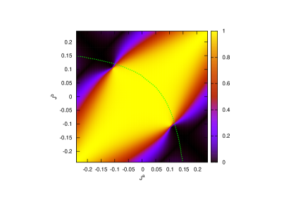
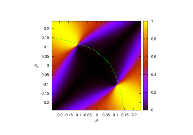
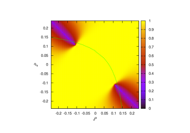
Figure 1: Exact diagonalization results for a square lattice with 2 by 2 sites, at $I/U=0.45$. The dashed green line in each plot marks the boundary between Mott and superfluid regime, obtained on the mean-field level as described in Section III.1.3. Left: Ground state magnetization with respect to $S_{z}=\frac{N_{A}-N_{B}}{N_{A}+N_{B}}$. Middle: Anticorrelation between nearest neighbors, measured by $P_{AB}=\sum_{\langle ij\rangle}\langle A_{i}^{\dagger}B_{j}+{\rm H.c.}\rangle$. Right: Overlap of the ground state with a product state, given by Eq. (19).

III.1.1 Limiting cases

Much of the physics can be understood by considering the limiting cases where $I$ and/or $J_{\pm}\rightarrow 0$.

For $J_{-}=0$ and $I=0$, the Hamiltonian (III.1) is equivalent to a ferromagnetic XXX model, with the states $\left|AA\right\rangle$, $\left|BB\right\rangle$, and $\left|AB\right\rangle+\left|BA\right\rangle$ forming a degenerate ground state manifold. The influence of a small but finite value of $I$ can be studied by a Taylor expansion: To first order, $I$ appears only in the term $\propto IS^{z}$, that is, it acts as a magnetic field. In that sense, this term defines the quantization axis of the ferromagnetic phase, and we accordingly define the magnetization $M$ as the averaged imbalance between atoms in state $\left|A\right\rangle$ and $\left|B\right\rangle$:

$$M=\sum_{i}\langle S_{i}^{z}\rangle/N.$$ (18)

With this definition we see that the states $\left|AA\right\rangle$ and $\left|BB\right\rangle$ are oppositely magnetized, $M=\pm 1$, while $\left|AB\right\rangle+\left|BA\right\rangle$ is unmagnetized, $M=0$. Clearly, at the onset of a small $I$, the degeneracy between these states is lifted through a linear Zeeman shift, $\Delta E\sim I\Delta M$. The unique ground state is then the fully magnetized one, $M=1$.

If we next also allow for small but non-zero $J_{-}$, we have, to lowest order in $J_{-}$, to take into account the last term in Eq. (III.1), $\propto S^{x}$. This term can be considered as an additional magnetic field component, so its presence will accordingly change the magnetization axis of the system. We thus expect a ferromagnetic phase with a continuously shifted quantization axis. With respect to the original quantization axis, this is reflected in a demagnetization, that is we get ground states with $M<1$.

Another limiting case which can be solved exactly is obtained by setting $I=0$, while taking $J_{-}$ and $J_{+}$ finite. In this case, the ground state reads $\left|+\right\rangle\equiv(\left|AA\right\rangle+\left|BB\right\rangle+\left|AB\right\rangle+\left|BA\right\rangle)/\sqrt{4}$ if $J_{+}J_{-}>0$, or $\left|-\right\rangle\equiv(\left|AA\right\rangle+\left|BB\right\rangle-\left|AB\right\rangle-\left|BA\right\rangle)/\sqrt{4}$ if $J_{+}J_{-}<0$. Both states are not magnetized, $M=0$.

An expression which is able to interpolate between all cases discussed so far is given by the product state ansatz

$$\left|\Pi(M)^{\pm}\right\rangle_{ij}\equiv\prod_{i}\left(\sqrt{\frac{1+M}{2}}\left|A\right\rangle_{i}\pm\sqrt{\frac{1-M}{2}}\left|B\right\rangle_{i}\right),$$ (19)

where magnetization $M$ is a free parameter. Apparently, independent of $M$, such ansatz describes ferromagnetic phases. The parameter $M$ accounts for the shift of the magnetization axis. More generally, one could still introduce a phase angle between the contributions $\left|A\right\rangle_{i}$ and $\left|B\right\rangle_{i}$. However, since in Eq. (III.1) the magnetic field along $S^{y}$ is always zero, the product wave function can be kept real.

A limiting case with very different physical behavior is given by $J_{+}\rightarrow 0$. The spin-spin interactions in Eq. (III.1) then yield an XYZ model, with ferromagnetic coupling in the $S^{x}$-direction, and antiferromagnetic coupling along the $y-$ and $z$-component of spin. To study this limit, we first consider the two-site Hamiltonian of Eq. (III.1): The two states $\left|AB\right\rangle$, $\left|BA\right\rangle$ are decoupled from the states $\left|AA\right\rangle$ and $\left|BB\right\rangle$. Their energy is given by

$$E_{\rm AB}=-dN\frac{2J_{-}^{2}}{U^{2}-4I^{2}},$$ (20)

where the prefactor $dN$ enables to go beyond the two-site picture by counting the number of nearest-neigbor pairs in a $d$-dimensional system of $N$ particles. The antiferromagnetic states compete with the ferromagnetic states $\left|AA\right\rangle$ and $\left|BB\right\rangle$. The ground state energy $E_{\rm FM}$ in the $\{\left|AA\right\rangle,\left|BB\right\rangle\}$ Hilbert space is found by diagonalizing a two-by-two matrix:

$$-dN\left(\begin{array}[]{cc}\frac{2J_{-}^{2}}{U+2I}+\frac{I}{d}&\frac{2J_{-}^{2}}{U}\\ \frac{2J_{-}^{2}}{U}&\frac{2J_{-}^{2}}{U-2I}-\frac{I}{d}\end{array}\right)\Psi=E_{\rm FM}\Psi.$$ (23)

By demanding $E_{\rm AB}<E_{\rm FM}$ we obtain the phase boundary between a ferro- and an antiferromagnetic phase. It is given by:

$$J_{-}^{\rm crit}/U=\sqrt{\frac{1}{d}}\sqrt{\frac{1-2(I/U)^{2}}{2\sqrt{2}}-\frac{1}{4}}.$$ (24)

This formula shows that larger dimensionality extends the antiferromagnetic regime towards smaller values of $I$ and $J_{-}$, that is, towards a parameter regime of best validity of the effective Hamiltonian Eq. (III.1).

III.1.2 Exact diagonalization results

The expectations from analyzing the two limiting cases are supported by a full numerical solution of the effective Hamiltonian for a small number of particles. We have considered chains (of up to 12 particles), squares of up to (16 particles), and a cubic arrangement of 8 particles. We calculated the ground state and low excitations by Lanczos diagonalization of $H_{\rm eff}$, and evaluated observables like ground state magnetization, defined in Eq. (18), and spin correlations. The latter we use, in particular, to identify antiferromagnetic order, which can be tested by an anticorrelation order parameter

$$P_{AB}\equiv\sum_{\langle ij\rangle}\langle A_{i}^{\dagger}B_{j}+{\rm H.c.}\rangle.$$ (25)

This quantity gives the probability of finding a particle in state $B$, once a neighboring site has been prepared in state $A$, and vice versa. It is unity only for the two chequerboard states.

As a test of the ferromagnetic behavior, apart from the magnetization with respect to $S^{z}$, we have calculated overlaps between the ground state and the product state ansatz of Eq. (19). The results are shown in Figs. 1 and 2 for small square lattices. Qualitatively, the same results are obtained for linear and cubic arrangement. Also the size of the system does not play a role. We could not find any qualitative influence of particle number on the calculated quantities, as long as it is kept even.

We find a broad regime in which the ferromagnetic solution (with $S^{z}$ quantization) is the ground state, see left panel of Fig. 1. However, for values $J_{-}\gtrsim J_{+}$, the magnetization decreases, but still, as evident from the right panel of Fig. 1, the system is in a product state. This confirms that quantization axis has shifted. We furthermore find that the sign $\epsilon=\pm$ in Eq. (19) is always defined by the sign of $J_{+}J_{-}$, $\epsilon=\frac{J_{+}J_{-}}{|J_{+}J_{-}|}$, as expected from the limiting case with $I=0$. Note that product states with + and - are physically distinguishable in the original basis of $a$ and $b$ particles. While states with $M=0$ and $M=\pm 1$ have, at least on average, the same number of $a$ and $b$ particles per site, state with $0<|M|<1$ have an excess of $a$ or $b$ particles, depending on $\epsilon$.

On the line corresponding to $J_{+}=0$ we find a sharp transition between a state with relatively large magnetization and small anticorrelations, and the chequerboard solution, characterized by $M=0$ and $P_{AB}=1$, see left and middle panel of Fig. 1, and left panel of Fig. 2. As a level crossing is the mechanism behind the transition, the transition is accompanied by a discontinuity in the first derivative of the energy as a function of $J_{-}$. Thus, along the line $J_{+}=0$, we have a second-order phase transition.

This is different from the transition which destroys the chequerboard order through the presence of a non-zero $J_{+}$. As shown in the right panel of Fig. 2, at constant $J_{-}$ the system smoothly evolves from an antiferromagnet to a ferromagnet. We note that the regime in which antiferromagnetic order dominates turns out to be very thin.

It should also be noticed that the chequerboard phase occurs only for relatively large values of $J_{-}/U$ and $I/U$. A discussion whether these parameters still allow for a Mott description will be given in Sec. III.1.3. In Fig. 1, we have anticipated the results from this section by drawing the Mott boundary (dashed line), obtained from the mean-field-like calculation presented below. We see that, at least for the concrete choice of parameters, the antiferromagnetic region coincides partly with the Mott region.

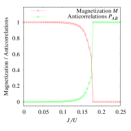
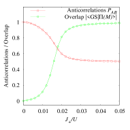
Figure 2: Exact diagonalization results for a square lattice with 4 by 4 sites, at $I/U=1/3$. Left: Ground state magnetization $M$ and anticorrelations $P_{AB}$, at $J_{+}=0$ as a function of $J_{-}/U$. Right: Ground state magnetization $M$ and overlap of the ground state with a product state, given by Eq. (19), at $J_{-}/U=0.2$ as a function of $J_{+}/U$

III.1.3 Mott-superfluid transition

In our analysis so far we have assumed that the system is in the Mott phase. For an estimation of the boundary between Mott and superfluid (SF) phase, we calculate the excitation spectra of the system. The occurrence of a zero-energy mode signals the breaking of U(1) symmetry, and thus the transition into the SF phase.

The excitation spectra are obtained from the Green functions, which we evaluate within the first order of a resummed hopping expansion dos Santos and Pelster (2009); Grass et al. (2011). This approximation is equivalent to a mean-field treatment, which for the standard Bose-Hubbard model is known to give quantitatively good results in $d>1$ dimensions.

Working in imaginary time, and Dirac picture, the time evolution of the operators reads

$$\hat{A}(\tau)= e^{H\tau}\hat{A}e^{-H\tau},$$ (26)

$$\hat{A}^{\dagger}(\tau)= e^{H\tau}\hat{A}^{\dagger}e^{-H\tau},$$ (27)

with $H=H_{I}+H_{0}$. With this we define the “deep Mott” (i.e. local) Green function as

$$G^{(\sigma,\sigma^{\prime})}(\tau,\tau^{\prime})= \sum_{N_{A},N_{B}=0}^{\infty}\frac{e^{-\beta E(N_{A},N_{B})}}{{\cal Z}^{(0)}}\times$$ (28)

$$\left\langle N_{A},N_{B}\right|\hat{T}\hat{O}^{(\sigma)\dagger}(\tau)\hat{O}^{(\sigma^{\prime})}(\tau^{\prime})\left|N_{A},N_{B}\right\rangle,$$

with $\beta$ the inverse temperature, ${\cal Z}^{(0)}$ the partition function of the system with $H_{J}=0$, $\left|N_{A},N_{B}\right\rangle$ a Fock state with $N_{A}$ ($N_{B}$) particles per site in state $A$ ($B$), $\hat{T}$ the imaginary-time ordering operator. The index $\sigma$ now stands for $A$ or $B$, and the operator $\hat{O}^{(\sigma)}$ is an annihilation operator with respect to the state $\sigma$. Note that in the $A,B$ basis, the Green function is diagonal. The object in Eq. (28) is most easily evaluated in Matsubara space. In the limit $\beta\rightarrow\infty$, the Green function reads

$$G_{i}^{(A,A)}(\omega_{\rm M}) =\frac{2}{U-\mu-I+i\omega_{\rm M}}-\frac{1}{-\mu-I+i\omega_{\rm M}},$$ (29)

$$G_{i}^{(B,B)}(\omega_{\rm M}) =\frac{1}{U-\mu-I+i\omega_{\rm M}}.$$ (30)

We can directly apply the formula from first-order resummed hopping expansion Grass et al. (2011); Graß et al. (2011):

$$[G_{\bf k}(\omega_{\rm M})^{(\sigma,\sigma^{\prime})}]^{-1}= \delta_{\sigma,\sigma^{\prime}}[G^{(\sigma,\sigma)}(\omega_{\rm M})]^{-1}-J^{(\sigma,\sigma^{\prime})}\times$$ (31)

$$[\cos(k_{x}a)+\cos(k_{y}a)+\cos(k_{z}a)].$$

Here, we have assumed a cubic lattice, but by neglecting the last cosine, the calculation is also carried out for square lattices. The poles of this Green function, i.e. the equation $[G_{\bf k}(i\omega)^{(\sigma,\sigma^{\prime})}]^{-1}=0$, yields the dispersion relations $\omega({\bm{k}})$.

In the regime of one particle per site we find three solutions which are gapped and behave quadratically around an extremum at ${\bf k}={\bf 0}$. Two of these modes are particle modes at positive energy, and the other is a hole excitation at negative energy. By increasing the hopping strength, at least one of the solutions becomes gapless, and the system becomes compressible. This marks the phase boundary of the Mott phase. For $I=J_{-}=0$, we obtain the standard (mean-field) Mott lobe. At the tip of the lobe, two modes become simultaneously gapless, marking the physical transition point to the superfluid regime. The internal hopping $I$ is found to simply shift the first Mott lobe from the interval $0<\mu/U<1$ to $-I/U<\mu/U<1-I/U$.

We are most interested in the regime where $J_{+}=0$. In this case, a relatively compact expression for the phase boundary is found:

$$J_{-}^{\rm MI/SF}(\mu,I)=\frac{1}{2d}\sqrt{\frac{I-I^{3}+\mu-2I\mu-I^{2}\mu-2\mu^{2}+I\mu^{2}+\mu^{3}}{1+I+\mu}}.$$ (32)

Here, all energies are expressed in units of $U$. At fixed $I$, this function gives the Mott lobe. Interestingly, the Mott boundary scales with dimension as $1/d$, while the antiferromagnetic boundary behaves as $\sqrt{1/d}$. Therefore, the parameter region of a possibly antiferromagnetic Mott phase is expected to be larger in system of less dimensions. Since the mean-field result is not reliable in 1D, we plot, in Fig. 3, the tip of the Mott lobe from Eq. (32) as a function of $I/U$ for a two-dimensional system. Also the antiferromagnetic boundary from Eq. (24) is plotted, and the shaded region marks a possibly antiferromagnetic Mott regime. It is restricted to relatively large values of $I/U\gtrsim 0.4$, where the validity of the effective Hamiltonian Eq. (III.1) is doubtable. We have to note, however, that for the standard Bose-Hubbard model it is well known that the mean-field calculation underestimates the Mott regime, with an error of around 30% in two dimensions. If this is the case also here, the antiferromagnetic Mott phase would extend to somewhat smaller values of $I$, cf. Fig. 3.

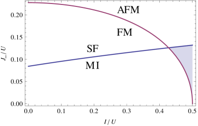
Figure 3: Phase boundaries of a 2D system at $J_{+}=0$: the blue line marks the (mean-field) boundary between Mott and superfluid phase. The purple line marks the phase boundary between an ferro- and antiferromagnetically ordered Mott phase. The shaded area marks the region in which an antiferromagnetic Mott phase is expected.

III.1.4 Experimental detection of the phases

The bare atomic states $a$ and $b$ can be distinguished by their different magnetic moment if one applies a real magnetic field along the quantization axis. In particular, within a time-of-flight expansion through such a field, this distinguishes between the $\left|+\right\rangle$ and the $\left|-\right\rangle$ phase. However, this does not allow to distiguish between the antiferromagnetic and the ferromagnetic $M=1$ phase, since both possess the same number of $a$ and $b$ particles. These phases can be distinguished by applying a magnetic field perpendicular to the quantization axis, with respect to which the two superpositions $A$ and $B$ posses opposite magnetic moments.

III.2 Magnetic ordering in SU(${\cal N}$) systems

We now turn to a discussion of SU(${\cal N}$) systems with ${\cal N}>2$. Due to the increasing Hilbert space, a full treatment becomes very tedious. We have seen for ${\cal N}=2$ that the most interesting physics occurs when $j_{\cal N}=J_{+}=0$, such that $j_{1}=J_{-}$ is the only contribution to the external hopping. To ${\cal N}>2$, this generalizes by choosing $j_{1}=j_{{\cal N}-1}^{*}$ different from zero, while all other hopping processes shall be zero. We further simplify the problem by choosing $j_{1}=j_{{\cal N}-1}\equiv j$ to be real.

With these simplifications, the Hamiltonian can be written as

$$H=-j\sum_{\langle ij\rangle,\sigma}\left(\hat{A}_{j}^{({\rm mod}[\sigma\pm 1,{\cal N}])\dagger}\hat{A}_{i}^{(\sigma)}+{\rm H.c.}\right)+H_{0}.$$ (33)

Here, every spatial hopping is connected to a hopping in the internal dimension. In SU(3), such a hopping term can be achieved by making $J^{(2)}=J^{(3)}$ and $J^{(1)}=-2J^{(2)}$. In SU(4), we have to make $J^{(1)}=-J^{(3)}$ and $J^{(2)}=J^{(4)}=0$.

Assuming again the Mott limit of one atom per site, we consider the effective Hamiltonians for the double-well problem. Let us denote the eigenstates of $H_{I}$ as $A,B$ for SU(2), $A,B,C$ for SU(3), and $A,B,C,D$ for SU(4). As explained before, the SU(2) system has a degeneracy between the state $\left|AB\right\rangle$ (that is with the left atom in $A$ and the right atom in $B$), $\left|BA\right\rangle$, and $(\left|AA\right\rangle+\left|BB\right\rangle)/\sqrt{2}$. This degeneracy is a consequence of the fact that $\left|AB\right\rangle$ and $\left|BA\right\rangle$ (or more generally: the two checkerboard states) are already eigenstates of a hopping which changes the pseudospin state by one. In contrast to this, a checkerboard solution does not exist for the SU(3) system. Accordingly, we find a unique ground state given by $(\left|AA\right\rangle+\left|BB\right\rangle+\left|CC\right\rangle+\left|AC\right\rangle+\left|CA\right\rangle+\left|AB\right\rangle+\left|BA\right\rangle+\left|BC\right\rangle+\left|CB\right\rangle)/3$.

The physics of the SU(4) system reduces to the SU(2) physics with three degenerate ground states in the two-site limit. This is not very surprising if we note that the Hamiltonian (33) is obtained from the original Hamiltonian $H_{I}+H_{J}+H_{0}$ by setting the hopping strength of two components to zero. In order to make the connection to the SU(2) case clearest, we define the local states $\left|a\right\rangle=(\left|A\right\rangle+\left|C\right\rangle)/\sqrt{2}$ and $\left|b\right\rangle=(\left|B\right\rangle+\left|D\right\rangle)/\sqrt{2}$. In terms of these states, the three degenerate ground states of the effective SU(4) Hamiltonian read $\left|ab\right\rangle$, $\left|ba\right\rangle$, and $(\left|aa\right\rangle+\left|bb\right\rangle)/\sqrt{2}$.

As already noted in Sec. II, for the right choice of $\phi$ in Eq. (3) it is possible to make the internal energies of the laser coupling, given by Eq. (6), equidistant. As argued before, this energy, divided by the coupling strength $I$, is somewhat similar to a magnetization of the state. We then find that $\left|a\right\rangle$ and $\left|b\right\rangle$ are states with opposite magnetization, just as the states $\left|A\right\rangle$ and $\left|B\right\rangle$ in the SU(2) case. Accordingly, the degeneracy will be lifted by $I$ in the same manner as discussed before, namely through a quadratic Zeeman shift.

IV SU(${\cal N}$) symmetry breaking in the interaction

Let us now discuss the case of $u\neq 1$, i.e. of the breaking of the SU$({\cal N})$-invariance already at the level of interaction. In particular, we focus on the region of parameters where $H_{J}$ couples the degenerate minima dominantly at second order in perturbation theory.

As derived and discussed in full detail in the Appendix A, for $0<U/U_{d}<1$ and for any $q\in{\mathbb{N}}$ it exists a non-zero window for the chemical potential, $\mu_{1}<\mu<\mu_{2}$, where the low-energy Hilbert space of the Mott phase is spanned by the states with $q+1$ particles in one species and $q$ in all the others. In formulas, these ${\cal N}$ normalized states are $\left|\bar{\sigma}\right\rangle\equiv\frac{{a^{\bar{\sigma}}}^{\dagger}}{\sqrt{q+1}}\left|q\right\rangle$, where $\left|q\right\rangle\equiv\sum_{\sigma}\frac{({a^{\sigma}}^{\dagger})^{q}}{\sqrt{q\!}}\left|0\right\rangle$ is the state of $q$ bosons for each species. This case is interesting as the perturbation theory in the spatial and species hopping induces a novel Potts-like effective Hamiltonian that displays different quantum phases.

IV.1 Effective Hamiltonian

Indeed, it is immediate to see that the hopping term in $I$ connects already at first order two vectors of the minima’s subspace while the term in $J$ can only act at second order in perturbation theory. This implies that interesting physics may appear within the range of validity of the effective Hamiltonian when $I/U$ and $J^{2}/U^{2}$ are of the same order of magnitude and much smaller than 1. As the Hilbert space where the effective Hamiltonian acts is ${\cal N}^{N_{L}}$ degenerate, $N_{L}\equiv$ number of sites, and it is generated by product states $\{\left|\bar{\bf\sigma}\right\rangle\equiv\prod_{i}\left|\bar{\sigma}(i)\right\rangle\}$, $H_{eff}$ can be written in terms of the matrix elements over such states

$$H_{eff}=\sum_{\bar{\bf\sigma}\bar{\bf\rho}}\left|\bar{\bf\rho}\right\rangle\left\langle\bar{\bf\rho}\right|H\left|\bar{\bf\sigma}\right\rangle\left\langle\bar{\bf\sigma}\right|=\sum_{\bar{\bf\sigma}\bar{\bf\rho}}\left|\bar{\bf\rho}\right\rangle H_{\bar{\rho}\bar{\sigma}}\left\langle\bar{\bf\sigma}\right|\,.$$ (34)

By denoting the creation (annihilation) operators in the neighborhood of the site $i$ as $a^{\dagger}_{il}$ ($a_{il}$), $l=1,\dots,2d$, the familiar expression for the matrix element is

$$H_{\bar{\rho}\bar{\sigma}}=-\sum_{i}\left(J^{2}\sum_{\bar{\bf\gamma},l,\sigma^{\prime},\rho^{\prime}}\frac{\left\langle\bar{\bf\rho}\right|a_{i}^{\sigma^{\prime}\dagger}a_{il}^{\sigma^{\prime}}\left|\bar{\bf\gamma}\right\rangle\left\langle\bar{\bf\gamma}\right|a_{i}^{\rho^{\prime}\dagger}a_{il}^{\rho^{\prime}}\left|\bar{\bf\sigma}\right\rangle}{\Delta_{\gamma}}\right.\\ \left.+I\sum_{\sigma^{\prime}}\left\langle\bar{\bf\rho}\right|\left(a_{i}^{\sigma^{\prime}\dagger}a_{i}^{\sigma^{\prime}+1}+a_{i}^{\sigma^{\prime}\dagger}a_{i}^{\sigma^{\prime}-1}\right)\left|\bar{\bf\sigma}\right\rangle\right),$$ (35)

where $\left|\bar{\bf\gamma}\right\rangle$ is any excited state obtained from a minimal energy state by acting with the hopping term on one link, and $\Delta_{\gamma}$ is the energy gap of such state. It is worth to notice that there are only four kinds of excitations. Indeed, there are two ways of adding a particle on one site: having two species with $q+1$ particles and the rest with $q$, let us call it $(++)$ configuration, or having one species with $q+2$ particles and rest with $q$, a $(2+)$ configuration. On parallel, when one particle is removed, we have a $q$ configuration, $q$ particles in each species, or a $(+-)$ configuration, with occupation $q+1,q-1,q\dots q$. In this language, the minimal energy configuration with $q+1$ particle in one species and $q$ for the rest is a $(+)$ configuration. Altogether, the four possibility are $\gamma_{++-+}$, $\gamma_{++q}$, $\gamma_{2+-+}$ and $\gamma_{2+q}$ (with the constraint that the $-$ occurs for the same species as the $+$ in the other site of the link), with the corresponding gap measured in units of $U$:

$$\Delta_{++-+}=1,\ \Delta_{++q}=u,$$ (36)

$$\Delta_{2+-+}=2-u,\ \Delta_{2+q}=1\,.$$ (37)

After some simple but lengthy calculation, one finds

$$H_{\bar{\rho}\bar{\sigma}}= -J^{2}\left(2N_{L}d\,A+B\sum_{i}\sum_{l=1}^{2d}\delta^{\bar{\sigma}(i)\bar{\sigma}(il)}\right)\mathds{1}-$$

$$\sum_{i}\Bigg{(}J^{2}C\sum_{l=1}^{2d}\delta^{\bar{\sigma}(i)\bar{\rho}(il)}\delta^{\bar{\rho}(i)\bar{\sigma}(il)}+I(q+1)\times$$

$$\left(\delta^{\bar{\sigma}(i)(\bar{\rho}(i)+1)}+\delta^{\bar{\sigma}(i)(\bar{\rho}(i)-1)}\right)\Bigg{)}\prod_{i^{\prime}\neq i,il}\delta^{\bar{\sigma}(i^{\prime})\bar{\rho}(i^{\prime})}\,.$$ (38)

The coefficients $A$, $B$ and $C$ are functions of the coupling $u\equiv\frac{U_{d}}{U}$, the number of species ${\cal N}$ and the total number of particles in each site $q{\cal N}+1$

$$A =\frac{q(q+1)({\cal N}-2)}{\Delta_{++-+}}+\frac{(q+1)^{2}}{\Delta_{++q}}+\frac{q(q+2)}{\Delta_{2+-+}}$$ (39)

$$=q(q+1)({\cal N}-2)+\frac{q(q+2)}{2-u}+\frac{(q+1)^{2}}{u},$$ (40)

$$B =\frac{q(q+1)}{\Delta_{++-+}}-2\frac{(q+1)^{2}}{\Delta_{++q}}-\frac{q(q+2)}{\Delta_{2+-+}}+\frac{(q+1)(q+2)}{\Delta_{2+q}}$$ (41)

$$=-\left(2(q+1)^{2}\frac{1-u}{u}+\frac{q(q+2)}{2-u}\right),$$ (42)

$$C =\frac{(q+1)^{2}}{\Delta_{++q}}=\frac{(q+1)^{2}}{u}.$$ (43)

Few comments on the above coefficients are in order. $A$ is just a constant shift of the energy and is always positive for the relevant region of the parameters’ space, ${\cal N}\geq 2$, $q\geq 0$ and $0<u<1$. The non-trivial part of the Hamiltonian is determined by the coefficient $B$ and $C$. $B$ is always negative in the relevant region of parameters’ space, and, with the exclusion of a small corner around $u\sim 1$, its modulus is bigger than $C$, which is always positive. In particular, in all parameters’ region it holds $|B|/C<2$: this has dramatic consequences on the nature of the ground-state, as it will be discussed in Sec. IV.2.

As a natural consequence of the periodic identification of the species, modulo ${\cal N}$, the effective Hamiltonian is $\mathbb{Z}^{\cal N}$ invariant. The implications of such invariance can be made transparent by rewriting the effective Hamiltonian in terms of operators. Following the notation of $\mathbb{Z}^{\cal N}$ lattice gauge theory Tagliacozzo et al. (2013), we introduce the unitary operators $X$ and $Z$

$$X\left|\sigma\right\rangle=e^{i\frac{2\pi}{\cal N}\sigma}\left|\sigma\right\rangle\rightarrow XX^{\dagger}=\mathds{1}$$ (44)

$$ZX=e^{i\frac{2\pi}{\cal N}}XZ\rightarrow Z\left|\sigma\right\rangle=\left|\sigma-1\right\rangle,\ Z^{\dagger}\left|\sigma\right\rangle=\left|\sigma+1\right\rangle\,.$$ (45)

By representing the states $\left|\sigma\right\rangle$ as unit vectors ${\bf v}_{\sigma}$ of components $v_{\sigma}^{a}={\delta_{\sigma}}^{a}$, the operators $X$ and $Z$ correspond to the ${\cal N}\times{\cal N}$ matrices $X=\rm{diag}\{e^{i\frac{2\pi}{\cal N}},e^{i\frac{4\pi}{\cal N}},\dots,e^{i\frac{2({\cal N}-1)\pi}{\cal N}},1\}$ and $Z_{ab}=\delta_{a{\cal N}}\delta_{b1}+\delta_{(a+1)b}$.

In order to implement the Hamiltonian Eq. 38, in terms of $X$ and $Z$, there are two main obstacles. The first is to construct the projector $P_{il}\left|\sigma_{i}\right\rangle\otimes\left|\sigma_{il}\right\rangle=\delta_{\sigma_{i}\sigma_{il}}\left|\sigma_{i}\right\rangle\otimes\left|\sigma_{il}\right\rangle$. Such an operator can be a function of $X_{i}$ and $X_{il}$ only, as it does not change the species. By noticing that $X_{i}\otimes X_{il}^{\dagger}\left|\sigma_{i}\right\rangle\otimes\left|\sigma_{il}\right\rangle=e^{i\frac{2\pi}{\cal N}(\sigma_{i}-\sigma_{il})}\left|\sigma_{i}\right\rangle\otimes\left|\sigma_{il}\right\rangle$, it is easy to verify that $P_{il}=\frac{1}{\cal N}\sum_{m=1}^{\cal N}(X_{i}\otimes X_{il})^{m}$. The second is the implementation of the exchange operator $R_{il}\left|\sigma_{i}\right\rangle\otimes\left|\sigma_{il}\right\rangle=\left|\sigma_{il}\right\rangle\otimes\left|\sigma_{i}\right\rangle$. Its action can be obtained by rotating simultaneously the spins using $Z_{i}\otimes Z^{\dagger}_{il}$ to the power $m=\sigma_{i}-\sigma_{il}$. Formally, it can be achieved for any $\sigma_{i}$ and $\sigma_{il}$ using the projector $P_{il}$, $R_{il}=\sum_{n=1}^{\cal N}(Z_{i})^{n}\otimes\mathds{1}_{il}\cdot P_{il}\cdot\mathds{1}_{i}\otimes(Z^{\dagger}_{il})^{n}$. As the term in $I$ is trivial, the Hamiltonian in the operator fashion is

$$H_{eff}=-\sum_{i}\left(J^{2}\sum_{l=1}^{2d}\left(BP_{il}+CR_{il}\right)+I\left(Z_{i}+Z_{i}^{\dagger}\right)\right).$$ (46)

IV.2 Exploring the phase space with a Gutzwiller ansatz

The ground state of the effective Hamiltonian (38) can be computed in the mean-field approximation using the Gutzwiller ansatz $\left|\Psi\right\rangle=\prod_{i}\left|\Psi_{i}\right\rangle$ with $\left|\Psi_{i}\right\rangle=\sum_{\sigma}f_{i}^{\sigma}\frac{a^{\dagger\sigma}}{\sqrt{q+1}}\left|q\right\rangle$, $\sum_{\sigma}|f_{i}^{\sigma}|^{2}=1$. As usual, the $f_{i}^{\sigma}$ are variational parameters that are determined by minimizing the expectation value of the effective Hamiltonian on $\left|\Psi\right\rangle$

$$\left\langle\Psi\right|H_{eff}\left|\Psi\right\rangle=\sum_{\{\bar{\sigma}\}\{\bar{\rho}\}}\left\langle\Psi\right|\left|\bar{\rho}\right\rangle\left\langle\bar{\rho}\right|H_{\bar{\rho}\bar{\sigma}}\left|\bar{\sigma}\right\rangle\left\langle\bar{\sigma}\right|\left|\Psi\right\rangle=$$

$$={\rm const.}-\sum_{i,\sigma}\Bigg{(}J^{2}\sum_{l,\rho}\left[f_{i}^{*\rho}f_{il}^{*\sigma}\left(Bf_{i}^{\sigma}f_{il}^{\rho}\delta_{\sigma\rho}+Cf_{i}^{\sigma}f_{il}^{\rho}\right)\right]+$$

$$(q+1)I\,\left[e^{i\phi}f_{i}^{*\sigma}f_{i}^{\sigma+1}+e^{-i\phi}f_{i}^{*\sigma}f_{i}^{\sigma-1}\right]+\lambda^{i}\left(\left|f_{i}^{\sigma}\right|^{2}-1\right)\Bigg{)},$$ (47)

where with an abuse of notation we include the Lagrange multipliers $\lambda^{i}$ to variationally impose the normalization of $\left|\Psi\right\rangle$ to one.

However, the main features of the ground-state of the effective Hamiltonian in the mean-field approximation can be understood without calculations. In particular, the phase diagram of the model can be read off by comparing the different terms that are competing and the relative strength of the corresponding coupling constant $B$, $C$ (which are controlled by $u$ and ${\cal N}$), and $I/J^{2}$. Let us start by describing the term sourced by $B$. Within the Gutzwiller ansatz it can written as $H_{B}\equiv\sum_{il\sigma}|f_{i}^{\sigma}|^{2}|f_{il}^{\sigma}|^{2}$, where the negative sign in the expectation value Eq. (47) is cancelled by the negative sign of $B$. As $H_{B}$ is positive definite its minimum corresponds to zero. It is evident that a checker-board-like configuration annihilates $H_{B}$, for instance $f_{i}^{\sigma}=\delta^{1\sigma}$, and $f_{il}^{\sigma}=\delta^{2\sigma}$. Such configuration can be consistently extended to the whole hypercubic lattice as it is bipartite. This tells us that whatever such term in the Hamiltonian dominates over the others the ground-state is not translational invariant. Now, let us consider the term sourced by $C$. This time we have $H_{C}\equiv-\sum_{il}|{\bm{f}}_{i}^{*}{\bm{f}}_{il}|^{2}$. As the ${\bm{f}}$ are normalized to 1, the modulus square of the scalar product can be at maximum 1, when the vectors are parallel or anti-parallel. This implies that the minimization of $H_{C}$ appoints to translational invariant configurations. In view of the above considerations, it is crucial to determine which of the two terms, and under which conditions, wins over the other. It is worth to notice that if translational invariance of the ground-state is assumed, this corresponds to uniform superposition of $\left|\sigma\right\rangle$ states, i.e $|f^{\sigma}|=1/\sqrt{\cal N}$ for any $\sigma=1,\dots,{\cal N}$, as obtained analytically by minimizing the fourth order polynomial. As the phases of the $f^{\sigma}$ are irrelevant we may choose for simplicity $f^{\sigma}=1/\sqrt{\cal N}$. Such observation allows us to derive an not rigorous argument to decide which is the actual ground-state depending on the relative values of $B$ and $C$ when $I=0$. The total energy per site of the translational invariant configuration above, $\left|\Phi\right\rangle=\frac{1}{\sqrt{\cal N}}\left|\sigma\right\rangle$, will be $E_{\Phi}=B/{\cal N}-C$. As a checker-board configuration has zero total energy, this means that $\left|\Phi\right\rangle$ is favorable whatever $E_{\Phi}<0$. For our effective Hamiltonian Eq. 38 this condition is always realized as $-B/C<2$. Hence, we conclude that the ground-state is translational invariant for $I=0$, at any value of ${\cal N}\geq 2$, $q\geq 0$ and $0<u<1$. The above argument is it not rigorous as a priori we cannot exclude the existence of less energetic and non-translational invariant configuration which it is not a minimum of $H_{B}$ and $H_{C}$ for separated, but the numerical evidence seems to discard such possibility.

Now, let turn our attention to the term source by $I$. As this is a local term, it is straightforward to find the translational invariant ground-state it selects. Depending on the value of $\phi$, it is a certain eigenvector of the circulant matrix, $(ZZ^{\dagger})_{\sigma\sigma^{\prime}}=\delta_{\sigma(\sigma^{\prime}-1)}+\delta_{\sigma(\sigma^{\prime}+1)}$, where ${\cal N}+1$ is identified with 1. For instance, for $\phi=0$ and $\phi=\pi$, it is the one corresponding to its maximal and minimal eigenvalues, respectively. As maximal eigenvalue and the corresponding eigenvector for any number of species are 2 and $f^{\sigma}=1/\sqrt{\cal N}$ for any $\sigma=1,\dots,{\cal N}$, respectively, the ground-state at $\phi=0$ is $\left|\Phi\right\rangle$ for any $I$ (by definition $I>0$).

In fact, the situation is more interesting for $\phi=\pi$, or for any other value providing a degeneracy of two eigenvalues. The former is equivalent to reverse the sign of $I$, and the eigenvector corresponding to the minimal eigenvalue has a non-trivial dependence on ${\cal N}$. In particular, for ${\cal N}$ odd there are two degenerate states with minimal intra-species hopping term, $\lambda_{min}=-2\cos(\pi/{\cal N})$, while for ${\cal N}$ even the state is unique, $\left|\Phi\right\rangle_{alt}=\frac{1}{\sqrt{\cal N}}\sum_{\sigma}(-1)^{\sigma}\frac{a^{\dagger\sigma}}{\sqrt{q+1}}\left|q\right\rangle$, with $\lambda_{min}=-1$. It is worth to notice that in the $d+1$ picture, where the different species correspond to layers in the compact extra-dimension (as the hopping in $I$ acts as a circular matrix where ${\cal N}+1$ is identified with 1), a negative $I$ implies the presence of a magnetic $\pi$-flux in the compact dimension.

In view of the above consideration, the existence of at least one phase transition is predicted within the mean-field approximation due to the hopping term between species. Indeed, starting with $I$ positive and decreasing it to negative values, the stable translational invariant phase determined by $\left|\Phi\right\rangle$, becomes metastable and a new translational invariant state takes over. If ${\cal N}$ is even, the ground-state is simply determined by $\left|\Phi\right\rangle_{alt}$. For ${\cal N}$ odd the situation is slightly more involved: The minimal local state is given by the linear combination of the two minimal eigenvectors of the circulant matrix that minimizes the effective Hamiltonian at $I=0$.

At this stage we cannot exclude the existence of other intermediate phases and corresponding phase transition. However, the above scenario is confirmed by numerical evidence. Let us analyze the results for even and odd numbers of species separately. In the former case, ${\cal N}=2r$, the state $\left|\Phi\right\rangle$ and $\left|\Phi_{alt}\right\rangle$ have the same energy contribution from $H_{B}$ and $H_{C}$, the transition happens exactly at $I=0$, for any value of $d$, $r$, $q$ and $u$.

In the latter, ${\cal N}=2r+1$, the main difference is that $\left|\Phi_{alt}\right\rangle$ is replaced by the linear combination of two minimal eigenvectors of $ZZ^{\dagger}$ which minimize $H_{B}$ and $H_{C}$. In fact, contrary to the SU$({\cal N})$-symmetric case, $u=1$, the interaction part of the Hamiltonian $H_{0}$ is not invariant under a change of basis to the eigenvalues of $H_{I}$ for generic $u$.

We conclude with two key observations. First, as in the SU$({\cal N})$-invariant case, checkerboard-like solutions can be achieved by considering species-dependent hopping term $H_{J}$. Second, again for any values of $u$, the different states and phases can be distinguished by time of flight experiment combined with a Stern-Gerlach one.

V Conclusion and Outlook

One of the major results we present here is that SU$({\cal N})$-breaking spatial hopping together with species mixing terms can induce inhomogeneous phases, i.e. the magnetization displays a crystal structure. Note that in the extradimension picture, in which the different pseudo-spin states become different sites, such pattern becomes a density pattern. Hence, the existence of Mott states of such sort suggests the presence of superfluid phases respecting the same crystal structure, i.e. supersolid phases. Such appearance is not totally surprising as the SU$({\cal N})$-symmetric interaction is long-range in the extradimension picture. In fact, a practical advantage of the synthetic dimension is that the long-range interaction is naturally not small. It is worth to notice that such scenarios naturally extend to approximately SU$({\cal N})$-symmetric interactions, which is more realistic for bosons.

Appendix A Minimal energy “Mott” states

For $J=I=0$, the Hamiltonian reduces to $H_{0}$, i.e.to the sum of local terms $H_{0}=U\sum_{i}h_{mott}(i)$ with

$$h_{mott}(i)=\sum_{\sigma}\left(-m\hat{n}_{i}^{\sigma}+\frac{1}{2}(\hat{n}_{i}^{\sigma})^{2}\right)+\frac{u}{2}\sum_{i,\sigma\sigma^{\prime}}\hat{n}_{i}^{\sigma}\hat{n}_{i}^{\sigma^{\prime}},$$ (48)

where $m\equiv\mu/U+1/2$ and $u\equiv U_{d}/U$. As minimizing $H_{mott}$ is equivalent to minimize each $h_{mott}(i)$, in what follows we omit for brevity the position index $i$. As $[h_{mott},\hat{n}^{\sigma}]=0$, we can minimize on the occupation basis and the number operators as numbers. Hence, it is convenient to identify the occupations of each species as the components of ${\cal N}$-vector ${\bf v}$, $v^{\sigma}=\hat{n}^{\sigma}$ and to express the quantity to be minimize as the algebraic problem:

$$h_{mott}=\frac{1}{2}{\bf v}^{\rm t}\cdot M\cdot{\bf v}-{\bf w}\cdot{\bf v}\,,$$ (49)

where $M_{\sigma\rho}=u+(1-u)\delta_{\sigma\rho}$, and $w_{\sigma}=m$, $\sigma,\rho=1,\dots\cal N$.

For any ${\cal N}$, $M$ is a real symmetric matrix that can be diagonalized to $diag\{1+({\cal N}-1)u,1-u,\dots,1-u\}$ in the following orthonormal basis

$${\bf e}_{1}=\frac{1}{\sqrt{\cal N}}(1,\dots,1)$$

$${\bf e}_{s}=(\overbrace{-\frac{1}{\sqrt{s(s-1)}},\dots}^{s-1},\sqrt{\frac{s-1}{s}},\overbrace{0,\dots}^{{\cal N}-s}),\ \text{\footnotesize$s=2,\dots,{\cal N}$}.$$ (50)

This implies that $h_{mott}$ becomes the sum of quadratic functions of each of the variables

$$X^{1}\equiv{\bf v}\cdot{\bf e}_{1}=\frac{\sum_{\sigma=1}^{\cal N}\hat{n}^{\sigma}}{\sqrt{\cal N}},$$

$$X^{s}\equiv{\bf v}\cdot{\bf e}_{s}=-\frac{\sum_{\sigma=1}^{s-1}\hat{n}^{\sigma}}{\sqrt{s(s-1)}}+\sqrt{\frac{s-1}{s}}\hat{n}^{s}.$$ (51)

By introducing $\nu=\sum_{\sigma=1}^{\cal N}\hat{n}^{\sigma}$ to indicate the total number of particle per site, we have

$$h_{mott}=\frac{1+({\cal N}-1)u}{2{\cal N}}\nu^{2}-m\nu+\frac{1-u}{2}\sum_{s=2}^{\cal N}(X^{s})^{2}\,.$$ (52)

It is straightforward to minimized the above expression, at least when $\nu$ is commensurable with number of species. Depending on the sign of the quadratic terms, we can distinguish 3 main regions. For $u<-1/({\cal N}-1)$, $h_{mott}$ is unbounded from the below as the system tries to acquire as many particles as possible for any value of the chemical potential. Precisely at $u=-1/({\cal N}-1)$, the energy of the system is not depending on the number of particles per site but only on their distribution between the different species.

For $-1/({\cal N}-1)<u<1$, both the terms in $\nu$ and $X$s are convex. If $m$ is such that $\nu=q{\cal N}$, for $q\in{\mathbb{N}}$, $m=m_{q}\equiv(1+({\cal N}-1)u)q$, the minimum is achieved at $X^{s}=0$ for any $s=2,\dots,{\cal N}$, i.e. for a uniform distribution of particles $\hat{n}^{\sigma}=q$, $\sigma=1,\dots,{\cal N}$. For a generic value of $m$, the terms in $\nu$ and $X$s compete. It can be shown that for $-1/({\cal N}-1)<u<0$ the system admits only the commensurable filling $\nu=q{\cal N}$ with uniform distribution per species, while for $0<u<1$ the system explores configurations with exceeding particles over the uniform distribution. In practice, if we increase $m$ starting from $m_{q}$, in the latter case the configuration with one particle added in any one of the species becomes less energetic than uniform configuration before $m$ reaches $m_{q+1}$ while in the former case it does not occur. Indeed, by relabeling the species to have the extra particle in last one, $X^{s}=0$, $s=2,\dots,{\cal N}-1$, $X^{\cal N}=\sqrt{({\cal N}-1)/{\cal N}}$, and the energy of such configuration is

$$E_{q,1} =\frac{1+({\cal N}-1)u}{2{\cal N}}(q{\cal N}+1)^{2}-m(q{\cal N}+1)$$

$$\ \ \ \ +\frac{(1-u)({\cal N}-1)}{2{\cal N}}$$

$$=E_{q}+\Delta_{q,1},$$ (53)

to be compared with,

$$E_{q+1} =(\frac{1+({\cal N}-1)u}{2}(q+1)-m)(q+1){\cal N}$$

$$=E_{q}+\Delta_{q,{\cal N}},$$ (54)

where $E_{q}=(\frac{1+({\cal N}-1)u}{2}q-m)q{\cal N}$ is the energy of the uniform distribution with $q$ particle per species, and $\Delta_{q,1}=-m+m_{q}+1/2$ and $\Delta_{q,{\cal N}}=(1/2(1+({\cal N}-1))(2q+1)-m){\cal N}$ are the gaps with respect to it of the configuration with an extra particle, and of the uniform distribution with $q+1$ particles per species, respectively. Hence, by imposing $\Delta_{q,1}\leq 0$ while $\Delta_{q,{\cal N}}>0$ for ${\cal N}>2$, the condition $0<u<1$ is found. The above statement can be rigorously proved by consider all the minimal energy configurations with total on-site occupation $q{\cal N}\leq\nu\leq(q+1){\cal N}$. Indeed, it can be shown that the energy associated to them is

$$E_{q,p}=\frac{1+({\cal N}-1)u}{2{\cal N}}(q{\cal N}+p)^{2}-m(q{\cal N}+p)+\frac{1-u}{2}p\frac{{\cal N}-p}{\cal N},$$ (55)

where $E_{q,0}=E_{q}$ and $E_{q,p}=E_{q+1}$. Accordingly, the gap

$$\Delta_{p} =E_{q,p}-E_{q}$$

$$=p\left(\frac{1+({\cal N}-1)u}{2{\cal N}}(2q{\cal N}+p)+\frac{1-u}{2}\frac{{\cal N}-p}{\cal N}-m\right),$$ (56)

turns out to be monotonically growing function of $p$ for $0<u<1$ and to be monotonically decreasing function of $p$ for $-1/({\cal N}-1)<u<0$.

The point $u=1$ separating the second region from the third region is special as it represents the SU$({\cal N})$ symmetric point. The energy simply depends on the $\nu$ and the ground state is as degenerated as all the possible ways of distributing $\nu$ particles in ${\cal N}$ boxes.

The third region, $u>1$, the quadratic term in the total occupation is positive definite while the one in the $X$s is negative definite, hence the minimum of the energy is obtained by maximizing the $X$s for fixed $\nu$. It is immediate to realize that this happens then all the particles seats in one species.

A.1 The ground-state degeneration and the effective Hamiltonian in perturbation theory

As our strategy is to find novel many-body effect with the reach of an effective theory approach, the most interesting regions of parameters are the ones displaying a degenerate ground-state. In particular, to be the effective Hamiltonian of physical significance, the hopping terms in $J$ and $I$ should act not trivially on the minimal energy subspace at low order in perturbation theory, let us say at most at second order. From the analysis of the previous section, the degeneration of the minima it is present for $u=-1/(1+({\cal N}-1)$ and $u>0$. In the former case, the situation in presence of just two species, ${\cal N}=2$, has been already studied in Trefzger et al. (2009). For a generic ${\cal N}$, the spatial hopping terms can act differently than the identity only at order ${\cal N}$, as this is the minimal number of particles to be moved and each hopping operation can move one.

In the latter case, similar reasoning applies when $u>1$ but this time the quantity that determines the order of perturbation is the on-site occupation. The most interesting case is for $0<u\leq 1$. Let us focus before on $0<u<1$. Here, as shown in previous section, for any positive integer $q$ and any $p$ between $1$ and ${\cal N}-1$ it exists a value of $m$ such that the minimal energy configurations have $\nu=q{\cal N}+p$ and correspond to ${\cal N}-p$ species populated by $q$ particles and $p$ species populated by $q+1$. The vector space spanned by such configurations is $\left(\begin{array}[]{c}{\cal N}\\ p\end{array}\right)$ and the spatial hopping term has non trivial matrix element at second order in perturbation theory. The case $p=1$ is extensively studied in the main text sect. IV.

As also discussed in the main text, sect. III, the SU$({\cal N})$ symmetric model $u=1$ has a very rich degeneracy any partition of $\nu$ in ${\cal N}$ has minimal energy. This makes a perturbative treatment in $J$ and $I$ difficult. However, it should be noted that in this case the hopping term between the species can be treaded exactly. Indeed, by a rotation of the Fock operators $a^{\sigma}$, which by definition is conserving the total number of particles $\nu$, such term can be transformed in a species’ dependent chemical potential $m^{\sigma}=m+I\lambda^{\sigma}$, where the $\lambda^{\sigma}=2\cos(2\pi(\sigma-1)/{\cal N})$ are the eigenvalues of the circulant matrix. This means that the final ground states is non degenerate if $I>0$ or ${\cal N}$ is even. For odd ${\cal N}=2r+1$, as the minimum eigenvalue of the circulant matrix is double degenerated, $\cos(2\pi r/{\cal N})=\cos(2\pi(r+1)/{\cal N})=-\cos(\pi/{\cal N})$, the vector space of degenerate minima is $\nu+1$ dimensional, and the problem becomes isomorphous to SU$(2)$ with the same chemical potential for the two species.

A.2 $p=1$ and second-order perturbation theory: the excited states and their gaps

Let us detail the perturbation theory in the case $0<u<1$ and $p=1$. We start by analyzing the effect of the hopping between different species. As its effect on a state is to move particle to the species nearby, this term has a non zero matrix element already at first order between two $\left|\sigma\right\rangle$ and $\left|\sigma^{\prime}\right\rangle$ defined in section IV, corresponding to the circulant matrix $(ZZ^{\dagger})_{\sigma\sigma^{\prime}}=\delta_{\sigma(\sigma^{\prime}-1)}+\delta_{\sigma(\sigma^{\prime}+1)}$, where ${\cal N}+1$ is identified with 1. On the contrary, the spatial hopping term has zero matrix elements between such states as it is not conserving the on-site particle number $\nu$. This means that we have to consider second order processes. All the possible excited states that enter in a process constitute a vector space. A basis for them can be obtained by applying the hopping to just one link on the link of a product states of $\left|\sigma_{i}\right\rangle$. Hence the non trivial part to be computed is of the form $a^{\dagger\sigma}_{i}a^{\sigma}_{il}\left|\sigma_{i}\right\rangle\left|\sigma_{il}\right\rangle$. From

$$a^{\dagger\sigma}_{i}\left|\sigma_{i}\right\rangle=\left((1-\delta^{\sigma\sigma_{i}}\sqrt{q+1}\left|\sigma_{i},\sigma\right\rangle+\delta^{\sigma_{i}\sigma}\sqrt{q+2}\left|(\sigma)^{2}\right\rangle\right),$$

$$a^{\sigma}_{il}\left|\sigma_{il}\right\rangle=\left((1-\delta^{\sigma\sigma_{il}}\sqrt{q}\left|\sigma_{il},(\sigma)^{-1}\right\rangle+\delta^{\sigma_{il}\sigma}\sqrt{q+1}\left|q\right\rangle\right),$$ (57)

where the compact notation $\left|(\sigma_{1})^{p_{1}},\dots,(\sigma_{r})^{p_{r}}\right\rangle$ indicates the normalized state with $q+p_{1}$ particles in species $\sigma_{1}$, $\dots$, $q+p_{r}$ particles in species $\sigma_{r}$, and $q$ particles in the remaining species, it is immediate to realize that there are 4 types of excited states of different energies. Indeed, the four types of a local states appearing in Eq. 57, $\left|\sigma,\rho\right\rangle$ and $\left|\sigma,(\rho)^{-1}\right\rangle$, for any $\sigma\neq\rho$, $\left|(\sigma)^{2}\right\rangle$ for any $\sigma$, and $\left|q\right\rangle$, for short $(++)$ and $(+-)$, $(2+)$ and $(q)$ respectively. Their energy gap with respect the minimal energy configuration are

$$\Delta_{++}=-m+\frac{1}{2}+q+\left(1+2q({\cal N}-1)u\right),$$

$$\Delta_{-+}=m+\frac{1}{2}-q-\left(1+q({\cal N}-1)\right)u,$$

$$\Delta_{2+}=-m+q+\frac{3}{2}+q({\cal N}-1)u,$$

$$-\Delta_{1}=m+q+\frac{1}{2}+q({\cal N}-1)u.$$ (58)

Hence, the corresponding four combination allowed for the excited states are

$$\Delta_{++-+}=\Delta_{++}+\Delta_{-+}=1,$$

$$\Delta_{++q}=\Delta_{++}-\Delta_{1}=u,$$

$$\Delta_{2+-+}=\Delta_{2+}+\Delta_{-+}=2-u,$$

$$\Delta_{2+q}=\Delta_{2+}-\Delta_{1}=1.$$ (59)

References

- Auerbach (1994) A. Auerbach, Interacting Electrons and Quantum Magnetism (Springer-Verlag, 1994).
-
M. Lewenstein et al. (2012)
M. Lewenstein,
A. Sanpera, and
V. Ahufinger,
Ultracold Atoms in Optical Lattices - Simulating
quantum
many-body systems (Oxford University Press, 2012). - Greif et al. (2013) D. Greif, T. Uehlinger, G. Jotzu, L. Tarruell, and T. Esslinger, Science 340, 1307 (2013).
- Hofstetter et al. (2002) W. Hofstetter, J. I. Cirac, P. Zoller, E. Demler, and M. D. Lukin, Phys. Rev. Lett. 89, 220407 (2002).
- Gorshkov et al. (2010) A. V. Gorshkov, M. Hermele, V. Gurarie, C. Xu, P. S. Julienne, J. Ye, P. Zoller, E. Demler, M. D. Lukin, and A. M. Rey, Nature Phys. 6, 289 (2010).
- Altman et al. (2003) E. Altman, W. Hofstetter, E. Demler, and M. D. Lukin, New Journal of Physics 5, 113 (2003).
- Demler and Zhou (2002) E. Demler and F. Zhou, Phys. Rev. Lett. 88, 163001 (2002).
- Imambekov et al. (2003) A. Imambekov, M. Lukin, and E. Demler, Phys. Rev. A 68, 063602 (2003).
- Yip (2003) S. K. Yip, Phys. Rev. Lett. 90, 250402 (2003).
- García-Ripoll et al. (2004) J. J. García-Ripoll, M. A. Martin-Delgado, and J. I. Cirac, Phys. Rev. Lett. 93, 250405 (2004).
- Barnett et al. (2006) R. Barnett, A. Turner, and E. Demler, Phys. Rev. Lett. 97, 180412 (2006).
- Dalibard et al. (2011) J. Dalibard, F. Gerbier, G. Juzeliūnas, and P. Öhberg, Rev. Mod. Phys. 83, 1523 (2011).
- Graß et al. (2011) T. Graß, K. Saha, K. Sengupta, and M. Lewenstein, Phys. Rev. A 84, 053632 (2011).
- Cole et al. (2012) W. S. Cole, S. Zhang, A. Paramekanti, and N. Trivedi, Phys. Rev. Lett. 109, 085302 (2012).
- Radić et al. (2012) J. Radić, A. Di Ciolo, K. Sun, and V. Galitski, Phys. Rev. Lett. 109, 085303 (2012).
- Boada et al. (2012) O. Boada, A. Celi, J. I. Latorre, and M. Lewenstein, Phys. Rev. Lett. 108, 133001 (2012).
- Liu et al. (2004) W. V. Liu, F. Wilczek, and P. Zoller, Phys. Rev. A 70, 033603 (2004).
- Eckardt et al. (2010) A. Eckardt, P. Hauke, P. Soltan-Panahi, C. Becker, K. Sengstock, and M. Lewenstein, Europhys. Lett. 89, 10010 (2010).
- Hauke et al. (2012) P. Hauke, O. Tieleman, A. Celi, C. Ölschläger, J. Simonet, J. Struck, M. Weinberg, P. Windpassinger, K. Sengstock, M. Lewenstein, et al., Phys. Rev. Lett. 109, 145301 (2012).
- Celi et al. (2014) A. Celi, P. Massignan, J. Ruseckas, N. Goldman, I. Spielman, G. Juzeliūnas, and M. Lewenstein, Phys. Rev. Lett. 112, 043001 (2014).
- Goldman et al. (2013) N. Goldman, G. Juzeliūnas, P. Öhberg, and I. B. Spielman, arXiv:1308.6533 (2013).
- Dudarev et al. (2004) A. M. Dudarev, R. B. Diener, I. Carusotto, and Q. Niu, Phys. Rev. Lett. 92, 153005 (2004).
- Juzeliūnas and Spielman (2012) G. Juzeliūnas and I. B. Spielman, New Journal of Physics 14, 123022 (2012).
- Hügel and Paredes (2013) D. Hügel and B. Paredes, arXiv:1306.1190 (2013).
- dos Santos and Pelster (2009) F. E. A. dos Santos and A. Pelster, Phys. Rev. A 79, 013614 (2009).
- Grass et al. (2011) T. Grass, F. dos Santos, and A. Pelster, Laser Physics 21, 1459 (2011).
- Tagliacozzo et al. (2013) L. Tagliacozzo, A. Celi, A. Zamora, and M. Lewenstein, Annals of Physics 330, 160 (2013).
- Trefzger et al. (2009) C. Trefzger, C. Menotti, and M. Lewenstein, Phys. Rev. Lett. 103, 035304 (2009).